A Multi-Modal Person Recognition System for Social Robots

Autonomous and Intelligent Systems Laboratory, School of Mechatronic Systems Engineering Simon Fraser University, Surrey, BC V3T 0A3, Canada
*
Author to whom correspondence should be addressed.
Appl. Sci. 2018, 8(3), 387; https://doi.org/10.3390/app8030387
Submission received: 16 January 2018
/
Revised: 15 February 2018
/
Accepted: 26 February 2018
/
Published: 6 March 2018
(This article belongs to the Special Issue Social Robotics)
Abstract
:The paper presents a solution to the problem of person recognition by social robots via a novel brain-inspired multi-modal perceptual system. The system employs spiking neural network to integrate face, body features, and voice data to recognize a person in various social human-robot interaction scenarios. We suggest that, by and large, most reported multi-biometric person recognition algorithms require active participation by the subject and as such are not appropriate for social human-robot interactions. However, the proposed algorithm relaxes this constraint. As there are no public datasets for multimodal systems, we designed a hybrid dataset by integration of the ubiquitous FERET, RGB-D, and TIDIGITS datasets for face recognition, person recognition, and speaker recognition, respectively. The combined dataset facilitates association of facial features, body shape, and speech signature for multimodal person recognition in social settings. This multimodal dataset is employed for testing the algorithm. We assess the performance of the algorithm and discuss its merits against related methods. Within the context of the social robotics, the results suggest the superiority of the proposed method over other reported person recognition algorithms.
1. Introduction
Recognizing people whom we have met before is an indispensable attribute that is often taken for granted, yet playing a central role in our social interactions. It is suggested that humans can remember up to 10,000 faces (persons); though this is an upper cognitive limit as an average person remembers far less faces—around 1000 to 2000 different faces (persons) [1]. Humans are also remarkable in seamless and fast completion of various perceptual tasks, including object recognition, animal recognition, and scene understanding, to name a few. Acclaimed neurologist and author, the late Oliver Sacks, opined that the human brain is far less “prewired” than previously thought. In his highly readable and masterfully written book, “the Mind’s Eye” [2], he talks about brain plasticity and how all the senses collectively contribute to form a perception of the world around us: “Blind people often say that using a cane enables them to “see” their surroundings, as touch, action, and sound are immediately transformed into a “visual” picture. The cane acts as a sensory substitution or extension”. Within this setting, we mostly recognize people from their faces, though other characteristics such as voice, body features, height, and similar attributes often contribute to the recognition process.
In the context of the social robotics, it is very much desired that social robots, like humans, effortlessly distinguish familiar persons in their social circles without any intrusive biometric verification procedure. Consider how we recognize members of our family, co-workers, and close friends. Their faces, voices, their body shape, and features, etc., are holistically involved in the recognition process and the absence of one or more of these attributes usually do not influence the outcome of the recognition. There has been a large body of research that employs one or more biometric parameters for person re-identification for applications such as surveillance, security, or forensics systems. These features/parameters are derived from physiological and/or behavioral characteristics of humans, such as fingerprint, palm-print, iris, hand vein, body, face, gait, voice, signature, and keystrokes. Some of these features can be extracted non-invasively, such as face, gait, voice, odor, or body shape. In a parallel development, there are significant and impressive research studies that are focusing on face recognition which are generally non-invasive; however, it is important to distinguish the problem of person recognition from the face recognition.
Motivated by the above and noting that the problem of person recognition in social settings has not been investigated as widely as the related problems of person re-identification and face recognition; we propose a non-invasive multi-modal person recognition system that is inspired by the generic macrostructure of the human brain sensory cortex and is specifically designed for social human-robot interactions.
The rest of the paper is organized as follows: in Section 2, we outline the current state-of-art in multimodal person re-identification and face recognition systems. In Section 3, we present the detailed architecture and implementation of the proposed perceptual system for person recognition application. We will then include simulation studies and discuss the merits of the algorithm as opposed to other related methodologies in Section 4. We conclude the paper in Section 5.
2. Related Studies
The main thrust of the paper is to address the problem of person recognition in social settings. The problem presents new challenges that are absent in person re-identification scenarios such as surveillance, security, or forensics systems. Among these challenges are how to cope with changes in the general appearance of a subject due to attire change, extreme face and body poses, and/or variation in lighting. These challenges are further compounded by the fact that a concurrent presence of all biometric modalities is not always guaranteed. Moreover, the social robot is expected to complete the recognition task relatively fast (within the range of human reaction time in social settings). In addition, intrusive biometric verification procedure obviously is ruled out for social human-robot interaction scenarios. Nevertheless, multimodal biometric systems that non-invasively extract physiological and/or behavioral characteristics of humans, such as face, gait, voice, and body shape features have been reported to solve the person re-identification problem in social settings [3,4,5,6]. In such applications, the problem is treated as an association task where a subject is recognized across camera views at different locations and times [7]. Due to the low resolution cameras and unstructured environments, these systems employ features such as, color, texture, and shape in order to identify individuals across a multi-camera network. However, these features are highly sensitive to variations in the subjects’ appearance such as outfit or facial changes.
A person recognition system solely relying upon face recognition leads to erroneous detection if facial or environmental features change—such as growing beard, or substantial occlusion, variation in lighting, etc. There are also reported studies based on soft-biometric features that are non-invasive and are not much affected if the subject appears in different clothing [8,9]. Though, these methods rely upon a single biometric modality to extract specific auxiliary features. The performance of such systems is dramatically deteriorated in the absence of that dominant modality. A significant effort has been devoted to use face information as the main biometric modality in multimodal biometric recognition [9,10,11]. Within these classifications, multimodal biometric person recognition systems were proposed in [3,12]. These multimodal algorithms included a mixture of face, iris, fingerprint, and palm-print features. However, most of these studies also require other biometric features that cannot be extracted without the active cooperation of the subject, such as fingerprints, iris, and palm-prints. Hence, the overall multimodal biometric systems developed in most research studies fall within the invasive biometric system category. In contrast to the above methodologies, we introduce a non-invasive algorithm that does not require the cooperation of the subject as a requirement for its proper operation.
Since gait can be extracted non-intrusively from a distance, it is considered as an important feature in developing person recognition systems. Gait is referred to as the particular manner in which a person walks and it is classified among the non-invasive attributes [13]. Zhou et al. [4] proposed a non-intrusive video-based person identification system based on integration of information from side face and gait features. The features are extracted non-invasively and fused at either feature level [4] or at the match score level [5]. In [3], the outputs of non-homogeneous classifiers, which are developed based on acoustic features from voice and visual features from face, are fused at the hybrid rank/measurement level to improve the identification rate of the system. Deep learning algorithms have also been used to address the problem of face recognition and action recognition, respectively [14,15]. Despite the fact that the above-mentioned studies are non-invasive multimodal biometric identification systems, the fusion methods that are employed in these systems require the concurrent presence of all biometric modalities for proper functioning, whereas the architecture that is reported in this paper relaxes this condition.
BioID [16] is a commercial multimodal biometric authentication system that utilizes synergetic computer algorithms to classify visual features (face and lip movements) and the vector quantifier to classify audio features (voice). The outputs of these classifiers are combined through different criteria to complete the recognition. In [8,17], facial information and a set of soft biometrics such as weight, clothes, and color were used to develop a non-intrusive person identification system, whereby the weight feature was estimated at a distance by the assessment of the anthropometric measurements that were derived from the subject’s image captured by a standard resolution surveillance camera. The overall performance of the system was affected by the detection rate of the facial soft biometrics. In [13], the height, hair color, head, torso, and legs were used as complementary parameters along with the gait information for recognizing people. In order to improve the recognition rate of the system, the authors selected sets of these features along with gait information to be manually extracted from a set of surveillance videos. An intelligent agent-based decision-making person identification system was also reported in [18]. The system achieved a recognition rate of 97.67% when face, age, and gender information were used and a recognition rate of 96.76% when fingerprint, gender, and age modalities were provided to the system. A recent survey paper provides an overview on using soft biometric (e.g., gender) as complementary information to primary biometrics (e.g., face) in order to enhance the performance of the person identification system [19]. Some researchers have applied multimodal biometrics systems to address related problems, such as action recognition [20], speaker identification [21], and face recognition [22].
The main shortcoming of these systems is that their different components require different time scales for proper operation, which limits their functionality in reaching decisions as compared to the human response time in different social contexts scenarios. For example, when the face is not detected due to extreme pose, partial occlusion, or/and poor illumination; the biometric features extracted from the face are not available and consequently the system fails to complete the recognition process. In contrast to these methods, the proposed approach overcomes this constraint by adjusting the threshold value of spiking neurons and exploiting available biometric features in order to compromise between the reliability of the decision and the natural perceptual time of the attended task (Section 3 of the paper).
Most of the aforementioned studies have been developed and discussed from a surveillance and security perspectives rather than the social human-robot interaction. Also, these person identification systems have been developed relying upon the combination of at least one dominant modality and a host of auxiliary biometrics or a mixture of invasive and non-invasive biometrics. Small number of research studies has tackled the problem of person recognition and face recognition in the context of cognitive developmental robotics [23,24]. We would like to emphasize that we present a person recognition algorithm incorporating multimodal biometrics features that is non-intrusive, is not affected by changes in appearance (i.e., outfit change), and works within the range of human social interaction rate (human response time). Moreover, all of the studies that were reported in multimodal biometric systems assume simultaneous presence of all the considered biometric features. This assumption is, however, relaxed in the proposed algorithm.
3. Architecture of the Person Recognition System
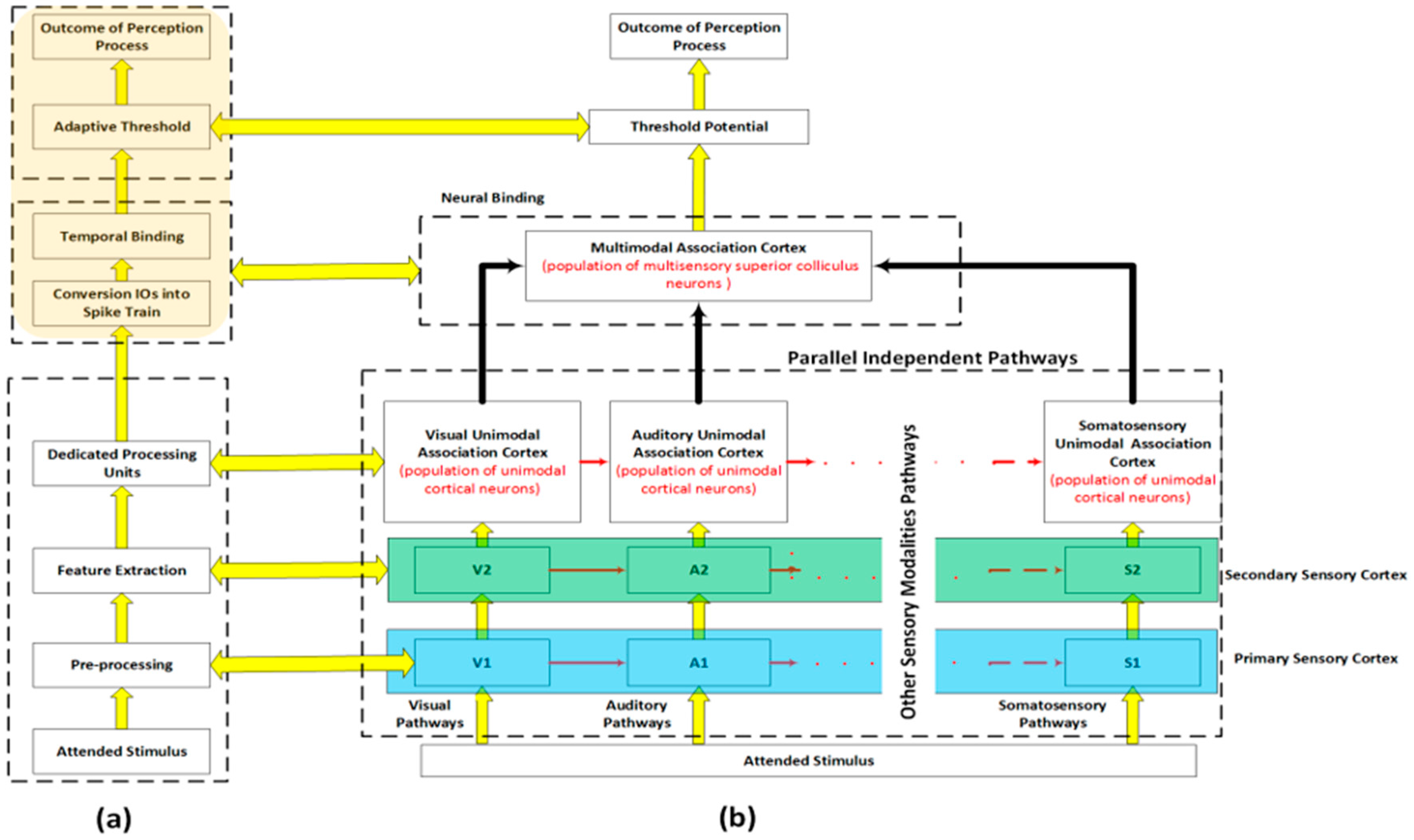
In this section, we present the architecture of the multi-modal person recognition algorithm in social settings. Figure 1 depicts the proposed system (Figure 1a) next to the architecture of the human/primate sensory cortex. Figure 1b shows a simplified architecture of the biological process as is widely accepted in neuroscience and psychophysics literature [25,26]. The architecture of the human sensory cortex is complex; it is thus naïve to claim an exact reconstruction. Within this pretext, Figure 1a shows our interpretation, which is a much simpler functional “engineered replica” with a one-to-one correspondence to the biological system. In particular, although the pathways for each modality in the human sensory cortex are parallel; there are strong couplings between these pathways particularly after the primary receptive fields. In addition, the human sensory cortex is directly involved in motivation, memory, and emotions. In the proposed architecture, we have neither included the coupling effects of modalities nor have we considered emotions and memory. However, we have strictly adhered to the spirit of the multimodal parallel pathways. As depicted in Figure 1b, an attended stimulus undergoes modality-specific processing (unimodal association cortex) before it converges at the higher level of the sensory cortex (multimodal association cortex) to form a perception [25,26,27,28,29].
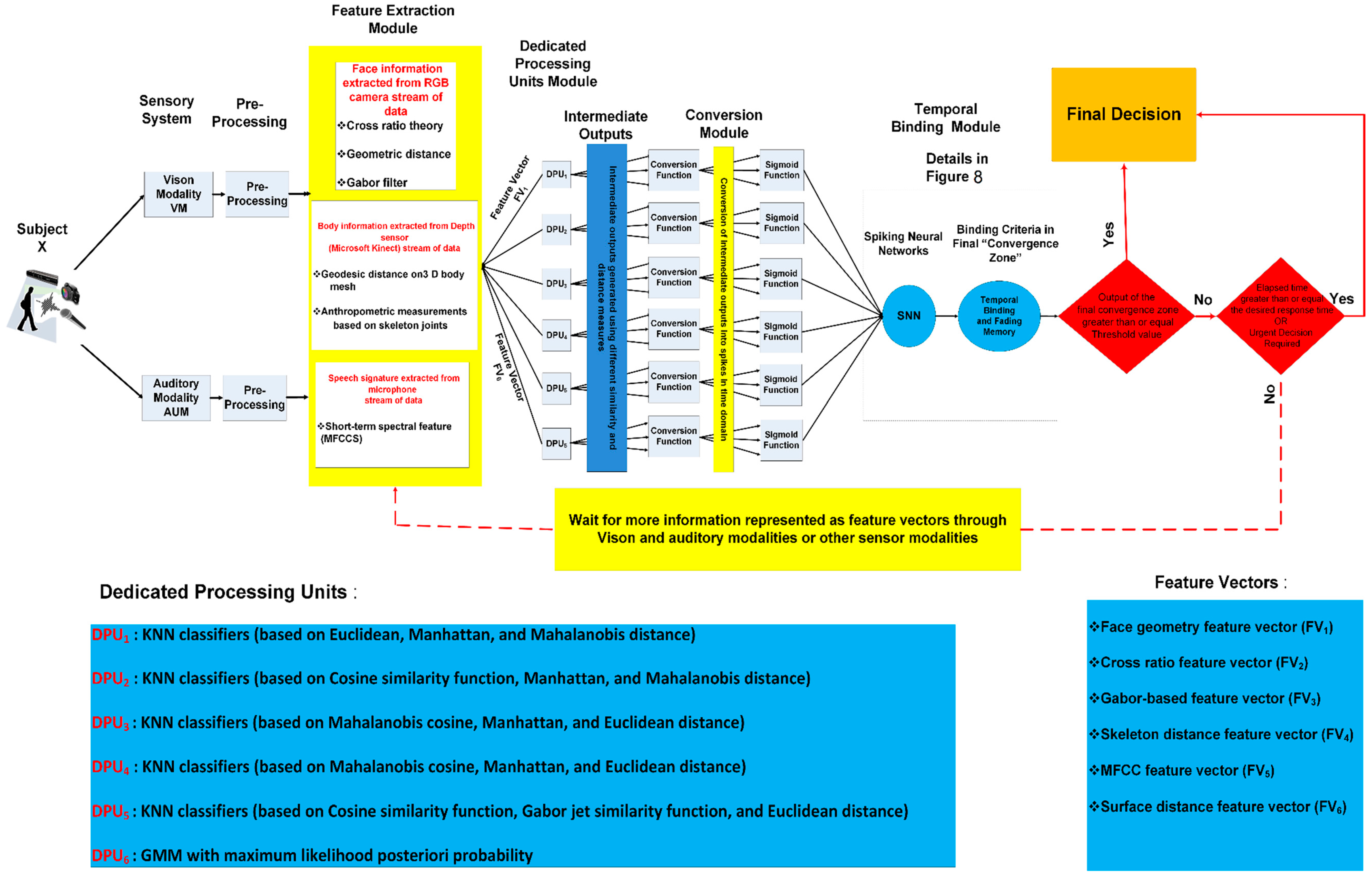
An attended stimulus to each of the visual, auditory, and somatosensory (touch, pressure, pain, etc.) systems undergoes a preprocessing and a feature extraction module, i.e., V1 and V2 in visual, A1 and A2 in auditory, and S1 and S2 in somatosensory pathways. When excited by a real-world stimulus, the corresponding neural systems of the human sensory system (vision, auditory, and tactile) map the stimulus’s attributes to available modalities. A similar structure is employed in the proposed system as elaborated in Figure 2 whereby each sensor modality and even different types of information within a sensor modality are processed in parallel and through independent processing pathways at the early stages of the perception process (feature extraction modules and dedicated processing units). The outputs of these independent pathways (intermediate outputs) converge at the higher level (temporal binding) to form the final outcome of the perception process. Also, in the biological system, an attended stimulus is mapped by population of neurons distributed across and within the cortical hierarchy, the binding or perceptual grouping is accomplished by synchronization of neural firings among population of neurons that form the cell assembly [26]. Then, the integration of the outputs of these cell assemblies in parallel with the search for the best match of the attended pattern, within the library of representations stored in memory, and perceive the attended stimulus. The findings from neuroscience and psychophysics suggest that the formation of cell assemblies is controlled by the following principles: (1) population of neurons in a specific cell assembly must have similar receptive field properties, (2) each cell assembly maps one feature or quality of the attended stimulus, and (3) population of neurons in the same cell assembly fire in temporal synchrony with each other.
We have incorporated these principles in the proposed architecture, as shown in Figure 1a and further elaborated in Figure 2. The first principle is depicted by connecting each sensory modality to a dedicated pre-processing and feature extraction module (corresponding to primary and secondary sensory cortex), which in turn generates a set of feature vectors representing different attributes of the attended stimulus. Feeding each of these feature vectors to its corresponding Dedicated Processing Unit (DPU) satisfies the second principle. Each feature vector is then processed by its respective DPU, which in turn, contributes to the production of the Intermediate Outputs (IOs). In the rest of this paper, we refer to the outputs generated by each DPU as simply IOs. The variation in the processing time that is required to generate the IOs and the availability of biometric modalities in the sensory system streams are handled by the binding modules. Psychophysics and psychological research studies suggest that the face recognition process uses two type of information: configural information and featural information, which are available at low and high spatial frequency, respectively. The former is used in early stage of recognition process and requires less processing time whereas the latter is used to refine and rectify the recognition process at the later stage and requires more processing time [30,31]. IOs will be transformed into temporal spikes in order to be processed by the temporal binding system. At the last stage, the output of the temporal binding module is compared with an adaptive threshold setting to either complete the perception process or to wait for more information from other sensor modalities. This adaptive threshold is controlled by two factors: the desired reliability of the final outcome and how fast a decision is required. In some scenarios, a fast response is more important than an accurate response; thus, the threshold will be reduced to accommodate such scenarios. For example, in the context of social robots, the natural (in the human sense) and relatively fast response is more desirable than an accurate but slow response [32]. In some situations, when an urgent decision is required, humans process a real-world stimulus by exploiting the most discriminant feature [33]. In such cases, a fast processing route is selected as the outcome at final convergence zone even the threshold value is not satisfied. However, in other situations when accurate response is more important than fast response, humans may take longer time and look for other cues to perceive reliably and accurately. The proposed framework accommodates both conditions by incorporating an adaptive threshold. The proposed architecture is customized to address the person recognition problem in social contexts, as shown in Figure 2. However, the same architecture may be adapted to solve other perceptual tasks that are vital in social robotics, including but not limited to, object recognition, scene understanding, or affective computing.
For the specific problem of person recognition, the architecture employs auditory as well as vision modalities. Though, the framework readily allows for the integration of additional modalities (tactile, olfaction) for other applications. As shown in Figure 2, when the sensory system (vision, auditory) is excited by a real-world stimulus, the corresponding receptive field system generate a map for the available stimulus’s attributes in a parallel manner. We refer to this stage in the architecture as pre-processing and feature extraction modules. It is well documented in psychophysics and neuroscience research where not only the processing of different sensor modalities is performed by independent routes of processing, but also different kinds of information within the same modality are processed by independent processing paths [26,34,35].
The capability of the perceptual system to finalize the perceptual task (person recognition in this study) in the absence of concurrent availability of all sensor modalities is utilized by using the spiking neurons in the binding modules (Section 3.4). For example, if the subject’s face is not available, then the binding module may use other available cues, such as body features, speech features, or both of them in order to finalize the recognition process within a reasonable response time (within the norm of the human response/reaction time). As depicted in Figure 2, a compromise between the reliability of the outcome and the requirement of quick response (in the order of human natural reaction) is achieved by an adaptive threshold (more on that in Section 3.4). We describe each module in more details in the rest of this section.
3.1. Front-End Sensors and Preprocessing
In order to address the person recognition problem, the visual and auditory pathways are employed. An RGB camera and a three-dimensional (3D) depth sensor (i.e., Kinect sensor) may be applied to capture the image and the corresponding depth information (vision modality/pathway), and a microphone could be employed to process the voice of a subject (auditory modality/pathway). The Kinect sensor as a 3D multi-stream sensor captures a stream of colored pixels; depth information associated with these colored pixels, and positioned sound. The data streams from the RGB camera, 3D depth sensor, and the microphone are processed via standard signal and image preprocessing (filtering and noise removal, thresholding, segmentation, etc.) to be prepared for the feature extraction module (Figure 2). In this study, however, such preprocessing is not required as we extract the input data from three databases that already provide preprocessed data.
3.2. Feature Extraction
In this section, we introduce the feature extraction stage, which is analogous to the primary and secondary sensory cortex in the human brain. The input of this module is the preprocessed data stream from the vision and auditory modules and its outputs are distinct feature vectors that will be processed by the respective classifiers as computational models for the DPUs (Figure 2).
The target application of the proposed person recognition system is social robotics. One of the most important and desirable attributes of the social robots is the ability to recognize individuals in various settings and scenarios, including challenging scenarios whereby one or more sensor modalities are temporary not available such as in vision system whereby lighting is inadvertently changed, or subjects change their outfits. Many reported methodologies have difficulties in coping with such unstructured settings.
In order to configure the perceptual system to person recognition tasks, three types of features, which are available in the data streams of auditory and vision system, need to be extracted. These features are categorized in three groups: the first group is based on spatial relationship, referred to as configural features; the second group is the appearance-based feature, which relies upon texture information; and the third group of feature is a voice-based feature which relies upon short-term spectral feature.
3.2.1. Vision-Based Feature Vectors
The vision-based feature vectors consist of two groups of feature vectors: The configural features group and the appearance-based feature group. Most of the feature vectors in the configural features are available early in the recognition process due to their relatively less computational requirements. On the other hand, the extraction of the appearance-based feature group is computationally expensive and is available later in the recognition process. This is also compatible with psychology and neuroscience findings that spatial information is processed early in the perception process and provides a coarse categorization scheme for an attended stimulus.
The Configural Features Group
The group consists of four feature vectors. The first feature vector is represented by the ratios of the Euclidian distances among the geometric position of a set of fiducial points on a face. These fiducial facial points are detected by “OpenFace”; an open source software for facial landmark detector [36]. The second feature vector is based on a cross ratio of the projection lines that are initiated from the corners of the polygon constructed from a set of predefined fiducial points on a face image. The third feature vector is constructed by computing the Euclidian distance among a set of selected skeleton joint positions. The fourth feature vector in this group is the surface-based feature, which is generated by computing the geodesic distances between the projections of selected pairs of skeleton joints on the point cloud that represent an individual’s body. It is worth mentioning that these feature vectors are purposely selected as they are easy to calculate and available early in perception process. The main purpose for these feature vectors are to limit the search scope and provide shortlisted candidates for the attended subject by biasing the top-ranked spiking neurons (see Section 3.4 for more details).
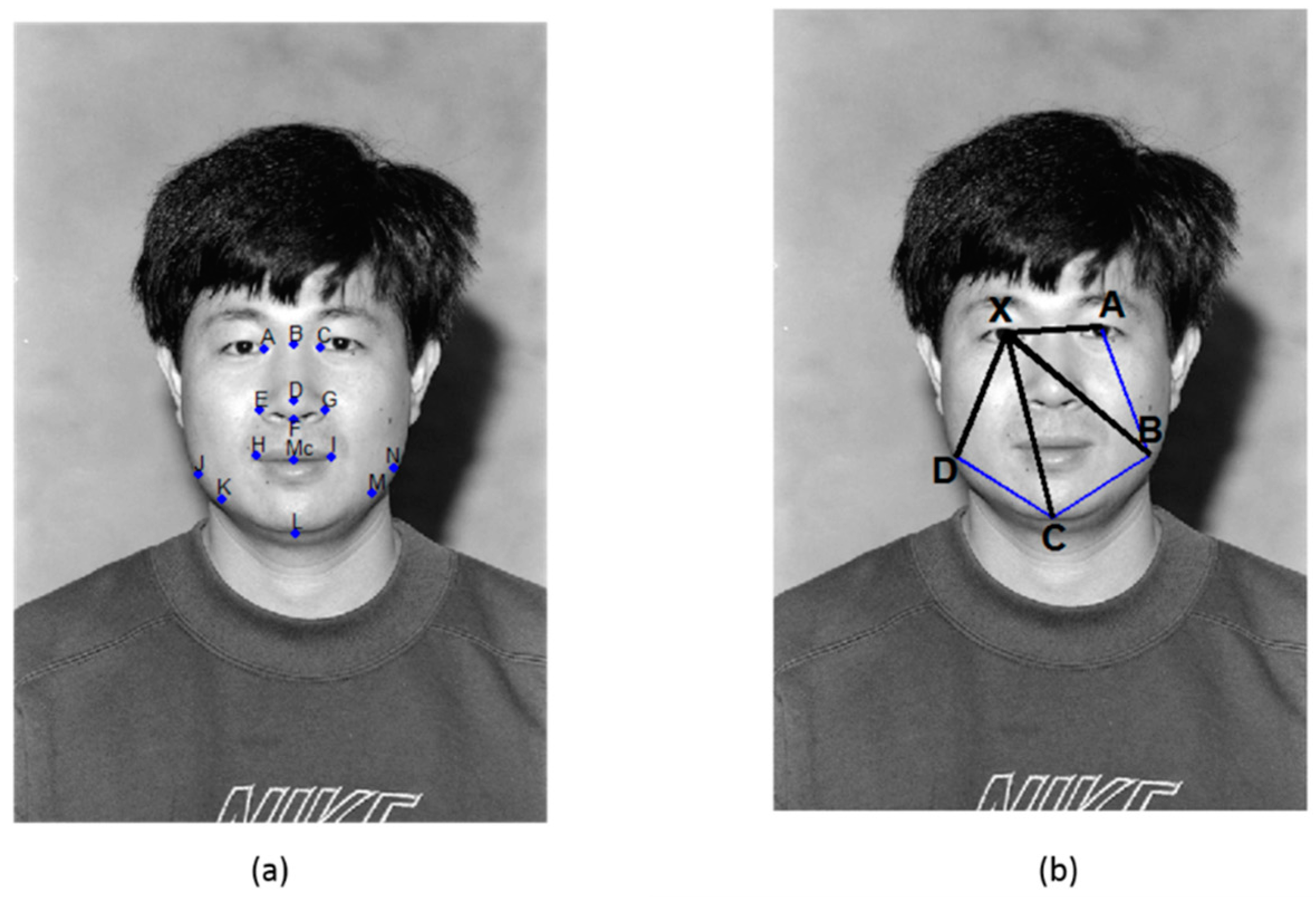
The first feature vector in the configural group consists of eight facial feature ratios, as shown in the Appendix A (Table A1). Despite the simplicity of this geometric descriptor, it can be shown that they generate comparable performance in face clustering with respect to other feature vectors that describe face appearance such as EigenFace and Histogram of Oriented Gradients [37].
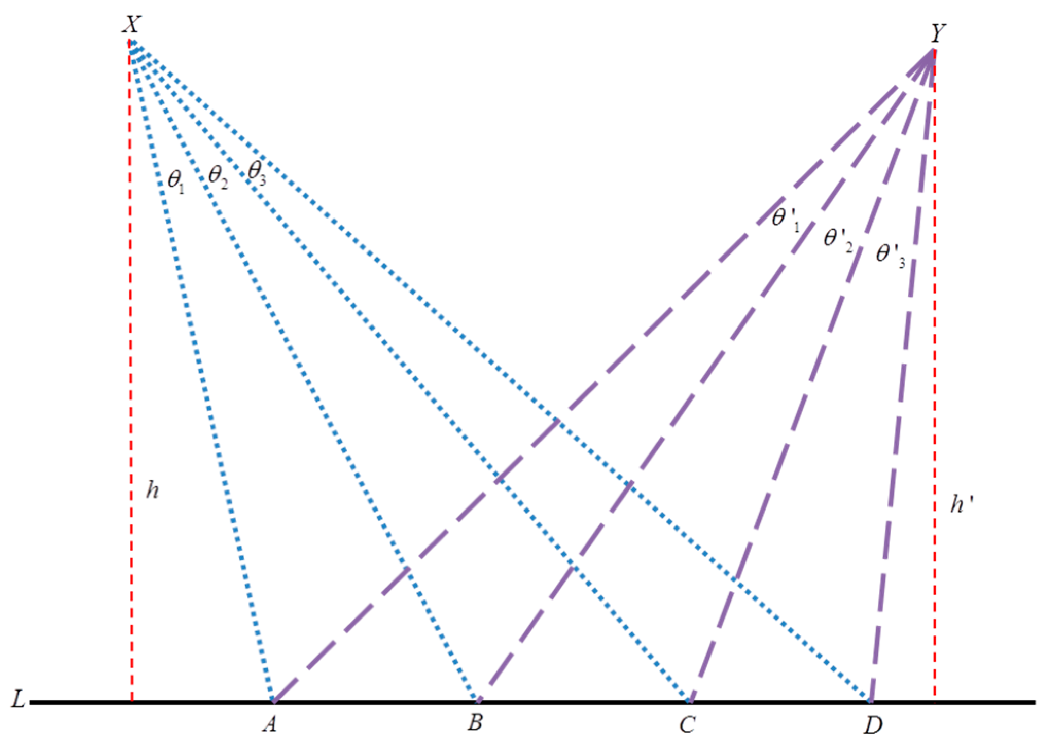
The second feature vector was constructed by employing the cross ratio theorem, which is a widely applied object and shape recognition algorithm in computer vision [38]. The cross ratio value stays invariant under geometric projection operations such as translation, rotation, and scaling changes [39]. The cross ratio of four collinear points A, B, C, and D in a line L, as shown in Figure 3, is given by:
The same cross ratio, , can also be expressed as ratio of the projection lines , , , and . By using the fact that the triangle area can be calculated using the formulas: and some algebraic manipulation, the cross ratio from point , can be expressed as a function of the line segments as in (1) or as a function of projection angles as in (2), where is the distance between the focus and the line AB, as depicted in Figure 3.
Since the cross ratio value is independent of changes in the viewpoint, the cross ratio of the same four collinear points A, B, C, and D in a line L from point Y can be expressed in the same way as point as in (3) and (4).
hence, . The reader may refer to [39] for detailed proof. Where and are two different viewpoints, represent the projection angles from point and respectively as shown in Figure 3.
The same principle is applied to measure the similarity of polygons that are constructed by selecting five points from the pre-defined fiducial points on a face image, as shown in Figure 4b. One fiducial point is used as the basis point and the other four must be non-collinear fiducial points to represent the polygon. The cross ratio of this polygon is regarded as the basis of similarity measure that is not affected by translation, scaling, rotation, and illumination. More details about the cross ratio for face recognition can be found in [39]. The set of five cross ratios is calculated by switching the basis point to one of the polygon’s corners, and the cross ratio values are obtained using (1) to (4).
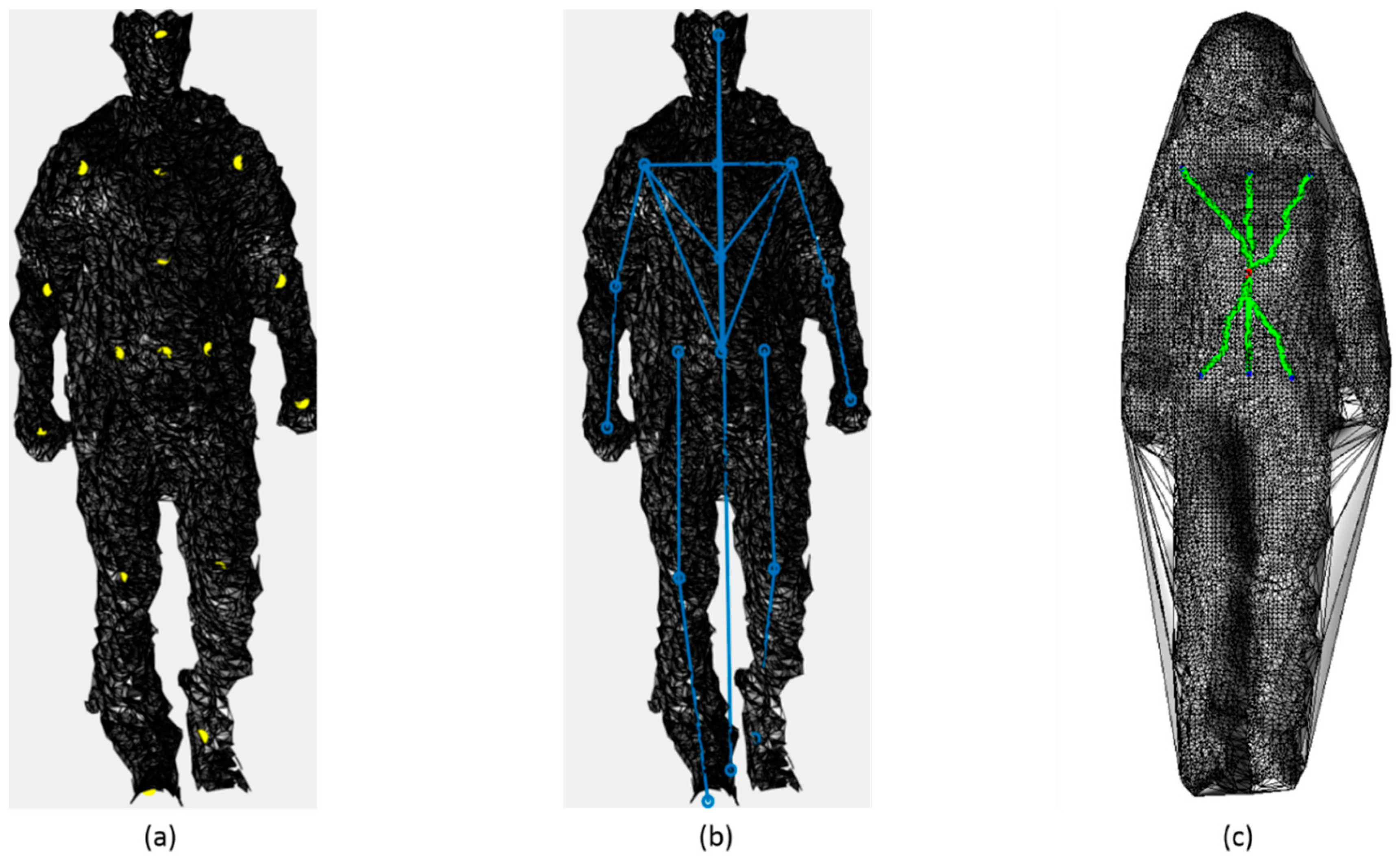
The third feature vector in this group is the skeleton-based feature. The combination of the distances between the selected skeleton joints, shown in Figure 5a, are used to generate this feature vector, as described in Table A2 and depicted in Figure 5b (The reader may refer to Appendix B for further details).
The surface-based feature vector is the last vector in the configural features group. This feature vector is computed using the combination of geodesic distances among the projection of selected skeleton joints on the three-dimensional body point cloud. First, the selected pairs of the skeleton joints, which do not usually lie on the point cloud, are projected on the associated closest point on the three-dimensional body mesh, which is generated from the point cloud. The pair of the projection points is used to initiate the fast-marching algorithm that provides a good approximation of the shortest geodesic path between two points on the surface. The fast-marching algorithm uses a gradient descent of the distance function to extract a good approximation of the shortest path (geodesic), as given by the Dijkstra algorithm [40]. Figure 5c depicts an example of geodesic distances used in constructing the surface-based feature vector. The selected geodesic distances that used to construct the surface-based feature vector are described in Table A3 (Appendix B).
The Appearance-Based Feature Group
The appearance-based feature consists of a set of multi-scale and multi-orientation Gabor filter coefficients extracted from the face image at fiducial points. The authors are aware of the availability of stronger descriptors like Scale-Invariant Feature Transform (SIFT) [41] and Speeded-Up Robust Features (SURF) [42], both of which can be used to generate feature vectors with high discrimination power. However, our intention is to process configural information early in the computation through an independent processing path in order to limit the number of candidates of an attended stimulus that can be refined further by the information available in the appearance-based feature. This interpretation is also compatible with the findings in neuroscience [34] and psychology [30] on human object and face recognition, suggesting that spatial information is used in early stages of the recognition.
The regional facial appearance patterns are normally extracted by the Gabor filter as a set of multi-scale and multi-orientation coefficients that represent the appearance-based feature vector. The Gabor filter may be applied to the whole face or to specific points on the face [43,44]. Extraction of Gabor filter coefficients is computationally expensive due to convolution integral operation; therefore, in order to speed up the computation, the Gabor filter coefficients are only computed at the fiducial points shown in Figure 4a. The two-dimensional (2D) Gabor filter centered at (0, 0) in the spatial domain can be expressed as in (5):
where and , and are spatial frequencies, and are the standard deviation of an elliptical Gaussian along the and axes, and represents the orientation. The Gabor filters have a plausible biological model to resemble the primary visual cortex. Physiological studies suggest that cells in the primary visual cortex usually have an elliptical Gaussian envelope with an aspect ratio of 1.5–2.0; thus, one can infer the following relation [45]:
Daugman [46] suggests that simple and complex cells in the primary visual cortex have plane waves propagating direction along the short axis of the elliptical Gaussian envelope. By defining the aspect ratio and assuming that the minimum value of aspect ratio is 1, the Gabor filter has an elliptical Gaussian envelope and the plane wave’s propagating direction along the , which is the shortest in case of , can be expressed as (6):
where and . Given an input image , the response image of the Gabor filter can be computed using the convolution operation defined as in (7). We convolve the image with every Gabor filter kernel in the Gabor filter banks centered at the pixels specified by the fiducial points.
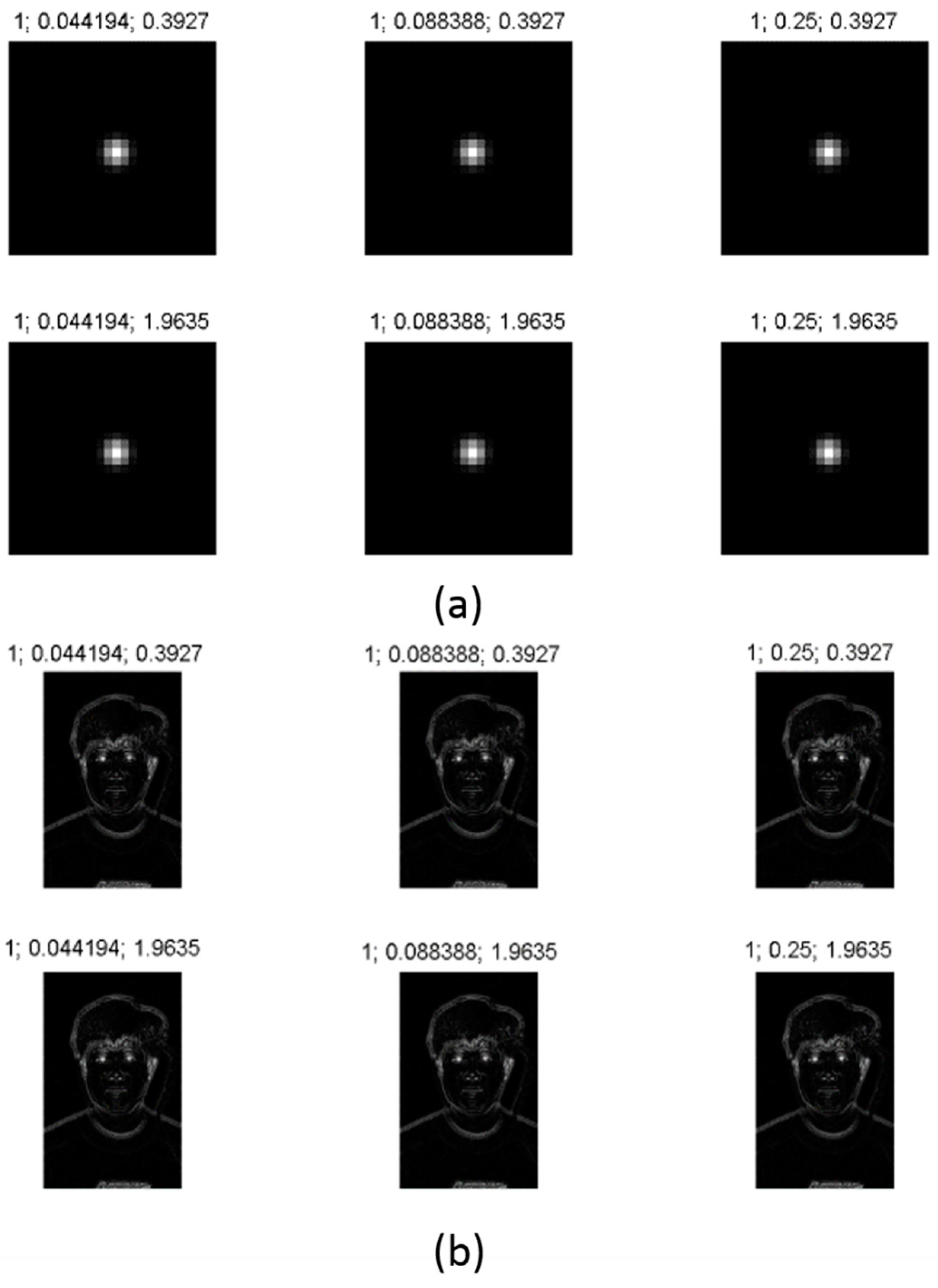
where is Gabor filter kernel centered at . is the intensity value of the image at location. The performance of the Gabor filter response in face recognition and classification tasks is highly affected by the parameters that are used in construction of the Gabor Kernel bank [44]. One of the well-known Gabor filter banks that is widely used in many computer vision applications especially object and face recognition tasks is the “classical bank”. The “classical bank” is characterized by eight orientations and five frequencies with Many previous studies have been devoted to addressing the problem of finding the Gabor filter parameters, which have optimum performance on the recognition tasks [43,47,48,49]. In this study, we adopted the Gabor filter parameters suggested by [44]. The author of that paper claims that the following parameterization of Gabor filter extracts the most discriminant information for recognition tasks. The suggested parameters are: eight orientations, six frequencies (instead of 5) with narrower Gaussian width ( instead of that is used in classical setting). The rest of the parameters were set the same as in the “classical bank” setting. The Gabor filter bank responses given in (7) consist of real and imaginary parts that can be represented as magnitudes and phases components. Since the magnitudes vary slowly with the position of fiducial points on the face, where the phases are very sensitive to them, we used only the magnitudes of the Gabor filter responses to generate the appearance-based feature vector. Hence, we have 48 Gabor coefficients for each fiducial point on the face. The selected set of Gabor filter kernels and responses are depicted in Figure 6; for demonstration, we selected one scale {1}, two orientations {}, and three frequencies { } to create Figure 6a,b. Figure 6a shows the magnitude of Gabor filtered kernels that were used to compute these coefficients at the fiducial points. Figure 6b depicts the magnitude of Gabor filter responses on a sample image from the FERET database (FERET database will be further discussed in Section 4).
3.2.2. Voice-Based Feature Vector
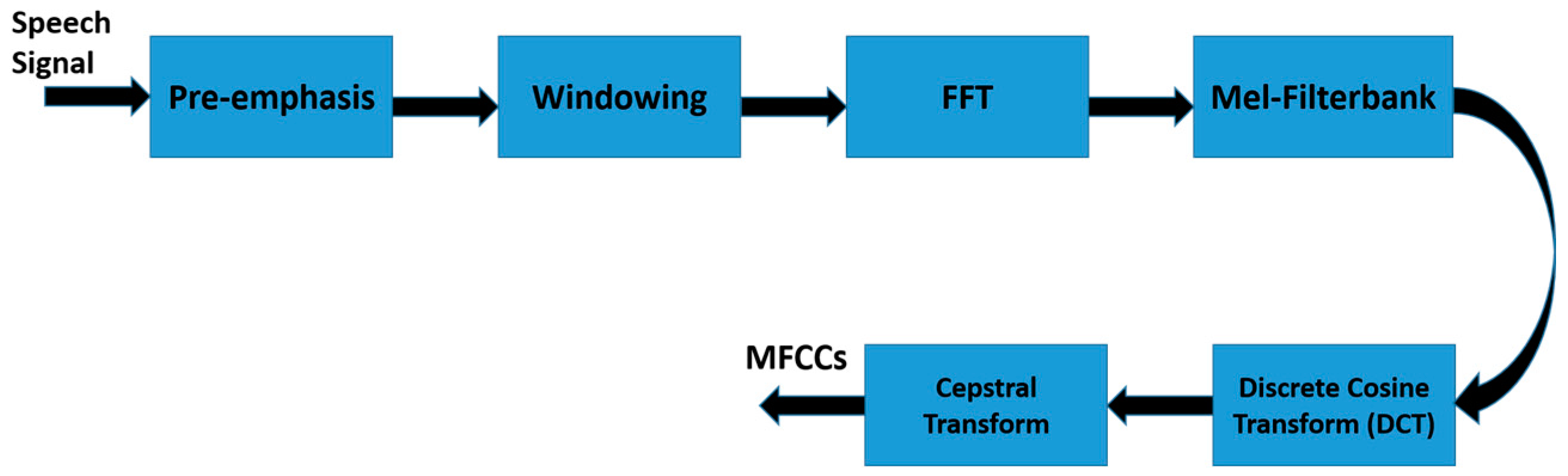
The voice-based feature vector is computed based on the short-term spectral, specifically, the so-called mel-frequency cepstral coefficients (MFCCs). We opted for MFCCs for many reasons: (1) MFCCs are easy to extract compared to other speech features, such as voice source features, prosodic feature, and spectro-temporal features; (2) MFCCs require relatively less amount of speech data to be extracted; and (3) MFCCs is text and language independent. Thus, MFCCs feature vector fits the nature of the person recognition for the social HRI where a real-time response and text-independent speech signature are crucial for user acceptance of social robot. A modular representation of MFCCs feature vector extraction is shown in Figure 7.
MFCCs feature vector is computed based on a widely accepted suggestion that the spoken words cover a frequency range up to 1000 Hz. Thus, MFCCs use linearly spaced filter at low frequency below 1000 Hz and logarithmic spaced filter at high frequency above 1000 Hz. In other words, the filter-bank is condensed at the most informative part of the speech frequency (more filters with narrow bandwidths below 1000 Hz) and lengthy-spaced filter-bank is applied at higher frequencies. As depicted in Figure 7, the first step in the extraction process is to pre-emphasize the input speech signal by applying filter as in (8).
where is pre-emphasized speech signal, is the input speech signal, and a pre-emphsized factor can be any value in the interval . In the next step (Windowing), the pre-emphasized speech signal is multiplied by smooth window function, here, we used Hamming windows, as in (9).
The resultant time-domain signal is converted to frequency domain by applying the well-known Fast Fourier Transform (FFT). The frequency range in the resultant FFT spectrum is very wide and fluctuated. Thus, the filter-bank that is designed according to Mel scale is applied in order to get the global shape of the FFT spectrum magnitude which is known to contain the most distinctive information for speaker recognition. The MFCCs are obtained by applying logarithmic compression and discrete cosine transform, as in (10). The discrete cosine transform converts log Mel spectrum into the time domain.
where is output of an M-channel filter-bank, is the index of the cepstral coefficient. In this study, we retained the 12 lowest excluding 0th coefficient.
3.3. Dedicated Processing Units and Generation of the Intermediate Outputs
As explained in the previous section, given a sequence of facial images, 3D mesh, and speech data for a person in various social settings, six feature vectors are extracted and considered to participate in the perception of an attended stimulus in order to recognize the person from different subjects in the database. The rationale for the choice of the six features is that the algorithm is architecturally and is functionally inspired by the human perceptual system. It is established that humans have limited channel capacity of processing the information from their sensory system. This capacity varies in the range of five to nine according to a seminal research study [50]. These feature vectors are: face geometry feature, cross ratio feature, skeleton feature, surface distance feature, appearance-based feature, and speech-based feature (Section 3.2). These features vectors are fed to DPUs in order to generate IOs. Selection of possible computational models of these DPUs is problem dependent and relies upon the perceptual task that needs to be addressed, as discussed in previous section.
3.3.1. Dedicated Processing Units for Vision-Based Feature Vectors
For the vision-based feature vector, we adopt classifiers that use various similarity and distance measures to represent their respective DPUs. These classifiers generate scores that evaluate how similar or close a subject is from those in the gallery. The interpretation of the best match relies on the types of distance and similarity measures that were used to generate these scores. For instance, in the case of various distance measures, such as L2Norm, L1Norm, Mahalanobis distance, and Mahalanobis Cosine; the minimum score represents the best match (please refer to Appendix A for more details). Whereas in cases where IOs are calculated using similarity measures, such as Cosine Similarity; the maximum score represents the best match. However, in order to unify these measures, such that the maximum score represents the best match; distance measures, they are further modified as (11).
where , represent various distance measures, IOjk is a unified score value representing how much the jth subject from the test set match or close to the kth subject from gallery set. It can be seen from (11) that the smallest distance yields a score value (IO) or a confidence value closer to one, while the largest distance value produces a very small score (IO) or a confidence value that is close to zero. These unified scores are then converted into spike times compatible with the inputs of neurons in the spiking neural network (SNN) at the next stage of hierarchical structure. For each subject in the test set, each feature vector participating in encoding the attended stimulus is processed by its respective DPU. In this study, DPUs are selected to be K-Nearest Neighbors (K-NN) classifiers which use a combination of three of the following similarity and distance measures: L2Norm, L1Norm, Mahalanobis distance, Mahalanobis Cosine, and Cosine Similarity as detailed in the architecture shown in Figure 2. Each DPU generates three matrices by adopting three of the aforementioned similarity and distance measures to compute scores for its associated feature vectors in the evaluation set against the corresponding feature vectors in the gallery set. However, only for the face appearance feature vector, the Gabor Jet Similarity measure of each subject in the evaluation set, is computed against the corresponding face appearance feature vector in the gallery set using (12) and (13).
where is the similarity between two jets, J and J′ associated with ith fiducial points on the face of the subject, is the amplitude of kth Gabor coefficient at ith fiducial points. N is the number of wavelet kernels. represents the total similarity between the two faces as the sum of the similarities over all the fiducial points as expressed in (13).
3.3.2. Dedicated Processing Units for Voice-Based Feature Vector
For the speech-based feature vector, MFCCs (mel-frequency cepstral coefficients) are used as an input to K-NN classifier with the aforementioned distance measures. Also, we used MFCCs that extracted from speech data of all of the speakers in the training data (gallery set) to create speaker-independent world model or a well-known universal background model (UBM). The UBM is estimated by training M-component GMM with the popular expectation–maximization (EM) algorithm [51]. The UBM represents speaker-independent distribution of the feature vectors. Here, we use 32-compnenent GMM to build the UBM. The UBM is represented by a GMM with 32-compnents, as denoted by , that characterized by its probability density function as (14).
The model is estimated by the weighted linear combination of D-variate Gaussian density function , each parameterized by a mean vector, , mixing weights, which is constrained by , , and a covariance matrix, as (15).
The purpose of training the UBM is to estimate the parameters of 32-component GMM, , from the training samples. The next step is to estimate specific GMM from UBM-GMM for each speaker in the gallery set using maximum a posteriori (MAP) estimation. The key difference between estimating the parameters of UBM and estimating the specific GMM parameters for each speaker is that the UBM uses standard iterative expectation-maximization (EM) algorithm for parameter estimation. On the other hand, specific GMM parameters are estimated by adapting the well-trained parameters in the UBM to fit a specific speaker model. Since the UBM represents speaker-independent distribution of the feature vectors, the adaptation approach facilitates the fast scoring, as there is a strong coupling between speaker’s model and the UBM. It should be noted that all or some of the GMM’s parameters ( can be adapted by MAP. Here, we adapted only the mean to represent specific speaker’s model. Now, Let us assume a group of speakers represented by GMMs . The goal is to find the speaker identity whose model has the maximum a posteriori probability for a given observation (MFCCs feature vector). We calculate the posteriori probability of all of the observations in probe set against all of the speakers models in gallery set as (16). As vary from 1 to number of speakers in the gallery set and the number of utterances in probe set, respectively, the result from (16) is matrix, namely . This matrix represents the IOs that are generated from speech-based feature vector and it will be integrated with other matrices that represent IOs generated from vision-based feature vectors.
Assuming equal prior probabilities of all the speakers, the terms and are constant for all speakerx, thus both terms can be ignored in (16). Since each subject in the probe set is represented as , thus by using logarithmic and assume independence between observations, calculation of can be simplified as (17).
Each feature vector generates IOs matrices, which provide a degree of support for each class in the gallery set based on several measures within the same feature vector. Also, IOs matrices that generated from different feature vectors provide a degree of support for each class in the gallery set in a complementary manner. The weight contribution of the IOs generated from the same feature vector to the final output is less than that of IOs generated from different feature vectors when they are integrated in the Spiking Neural Networks (SNN). This will be further discussed in the next section.
The next problem is to distinguish a subject x from the M subjects in the gallery set. Several IOs matrices are calculated for vision-based feature vector to be integrated with IOs matrices generated from the speech-based feature vector. Each matrix takes the size of a M × C matrix and its name is formatted based on the feature vector that generated it. The matrix name is read as . For example, the matrices that are describing the resultant IOs based on the skeleton feature vector should read as , where M represents the number of subjects in the gallery set and C is the number of samples in test set.
where is the IOs vector, represents how much the jth subject from the test set match or close to the kth subject from gallery set. This score is associated with a specific feature vector and is generated based on a certain distance measure that is specified by the name of the matrix.
3.4. Temporal Binding via Spiking Neural Networks
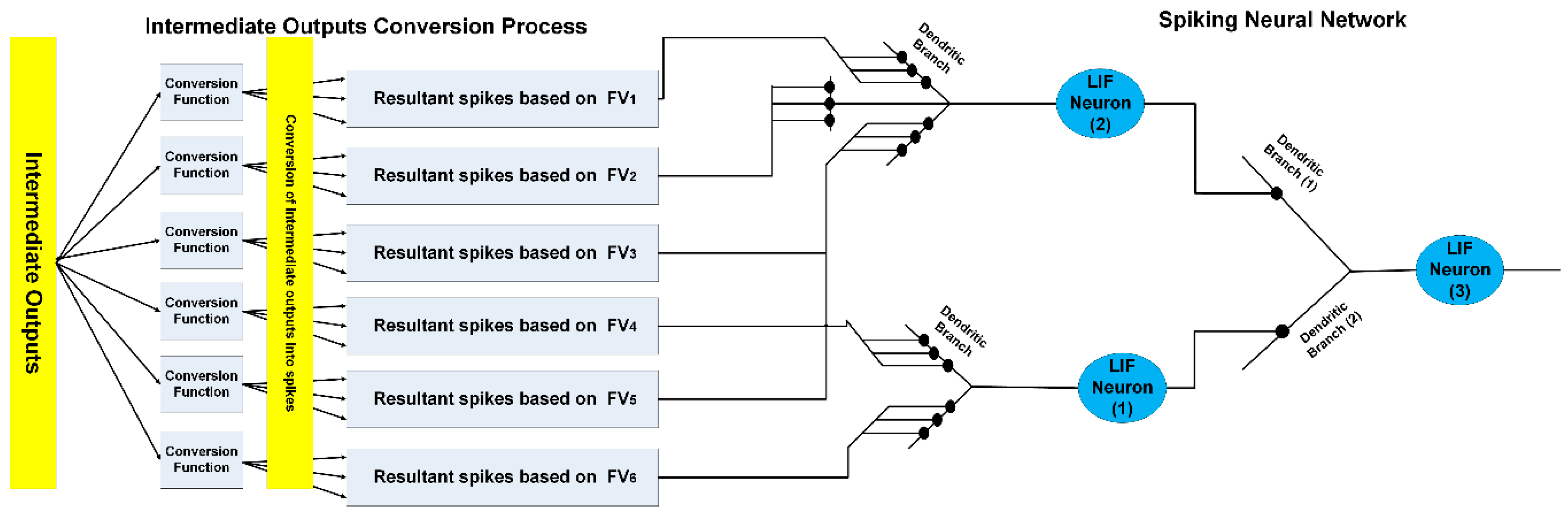
It is known that humans interact with their environment by processing the available information through multisensory modality streams over time with fading memory property. The same process is emulated here. In the context of this algorithm, fading memory implies that the effect of stimuli excitation (represented by IOs) deteriorates moderately if it is not reinforced or refreshed. We implement this feature through the Leaky Integrate-and-Fire neuron (LIF) model [52] to manifest the integration of IOs that are generated in the previous stage in the hierarchical architecture of the proposed system. Figure 8 depicts one block of the spiking neural network (SNN) that is used to perform the integration process. The overall SNN that is used to integrate the information from various biometric modalities is constructed by laterally connecting N blocks from the circuit, as shown in Figure 8, where N represents number of subjects in gallery sets.
The IOs vectors are fed to LIF neurons in SNN by means of pre-synaptic input spikes, as shown in Figure 8. IOs vectors, which are generated based on different feature vectors, are fed to independent branch in the dendritic tree. On the other hand, IOs vectors that are generated based on same feature vectors are fed to same branch in the dendritic tree. Inspired by neuroscience research studies [53,54], we suggest that the effect of presynaptic inputs on postsynaptic potential is either sublinear, super linear, or linear. The effects sum sub-linearly, linearly, or super-linearly if they are delivered to the same dendritic branch (within-branch) and sum linearly if they are delivered to different dendritic branches (between-branch). Equation (18) describes the dynamic of postsynaptic potential of LIF neuron. The dynamic of this neuron can be described as follows: initially at time t = 0, Vm is set to Vinit. If Vm exceeds the threshold voltage Vthresh, then it fires a spike and it is reset to Vreset and held there for the length Trefact of the absolute refractory period. The total response of postsynaptic potential due to different presynaptic inputs within-branch () and between-branch () is computed using (18) to (20).
where is the membrane time constant, is the membrane resistance, is the current supplied by the synapses, is a Gaussian random variable with zero mean and a given variance noise, Vm is the membrane potential of LIF neuron, Vinit is the initial condition for Vm at time , and Vthresh is the threshold value. If Vm exceeds Vthresh, then a spike is emitted, Vreset is the voltage to reset Vm to after a spike, and is the membrane potential of LIF neuron at no activity.
where represents the total input to the ith dendritic branch, is the ith dendritic branch weight, is the number of dendritic branches. Note that the sigmoid function is one possible choice of synaptic integration function within-branch and can be replaced with other functions, such as hyperbolic tangent sigmoid function.
It can be noted from (19) and (20) that the balanced IOs that are delivered to same dendritic branch will sum as follows: (1) small IOs will sum nearly linearly, (2) around average IOs will sum super-linearly, (3) large IOs will sum sub-linearly. Unbalanced IOs fed to the same branch generate near-linear summation over the entire range of IOs intensities. Moreover, IOs that are delivered to independent branches will sum linearly for all of the combinations of IOs intensities. Synaptic integration in dendritic tree of pyramidal neuron was experimentally proved to demonstrate similar behavior to the aforementioned forms of summations [55]. These forms of summations provide a tradeoff between error variance and error bias. Sub-linear summation of within-branch IOs, in case of large IOs, reduces the error variance by not exaggerating the effect of one aspect of the measure at the expense of other measures in deriving the final outcome. In addition, the linearly weighted aggregation of between-branch IOs reduces error bias by means of exploiting various attributes in deriving the final outcome.
As shown in Figure 8, the integration of IOs is performed using SNN in time domain to emphasize the temporal binding with fading memory criteria. The IOs represent various scores of confidence; each one of them provides a degree of support for each subject in the gallery set according to a certain aspect of measure and based on a specific biometric modality. These scores are introduced to SNN as presynaptic inputs by means of spikes fired at different times. As described in the previous section, all of the IOs are unified such that high score is equivalent to best match. In order to introduce the IOs to LIF neurons, the IOs are converted to spike times using (11) such that a high IO is equivalent to early firing time. Hence, the neuron which fires first represents the best candidate of the attended subject (from the gallery set). As LIF neurons receive early spikes, which correspond to high degree of support, their membrane potential U increases instantaneously. Once the membrane potential U of one of these neurons crosses the threshold value , the neuron fires a spike and all neurons participating in the process are reset to . The neuron which fires a spike first, which we refer to as the winner neuron, represents the best candidate of the attended subjects, and the attended subject is labeled with class number assigned to that neuron.
The threshold value of the neurons in the SNN controls both the reliability of the perception outcome and the allowed for the perception time of the attended task. A LIF neuron with a high threshold value implies that it will not fire until high intensity presynaptic inputs are delivered to its dendrite branches. These presynaptic inputs may be not available due to the absence of some biometric features or the need for more processing time. Thus, a compromise between the reliability and the reasonable perception time can be achieved by controlling the threshold value, according to a specific scenario of social interaction. As IOs are introduced to LIF neurons in parallel (Figure 8) via presynaptic inputs, one very high IO may drive a neuron to fire a spike and finalize the perception process. This sheds light on the superior feature of this model, such that one biometric feature with high discriminant power may be enough to finalize the perception process. This feature replicates the ability of humans to recognize odd features very quickly [56]. In the face perception and recognition, humans focus on distinctive features, which correspond to very high IOs in this algorithm so that other features may not need to be used.
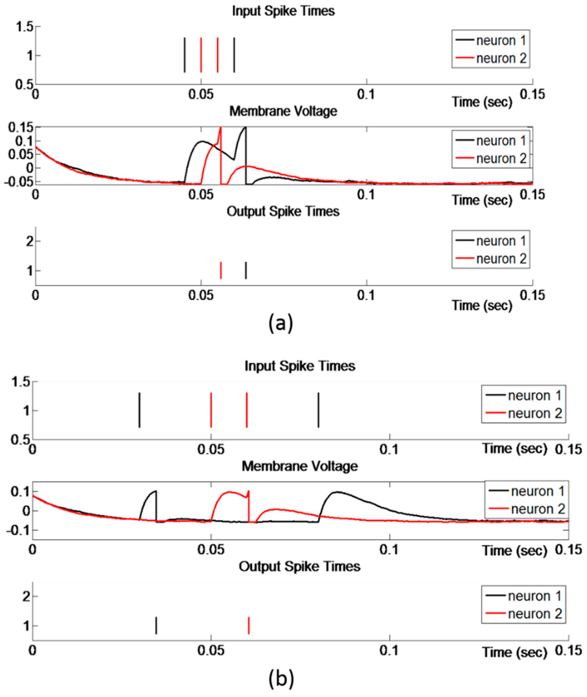
Another vital property of this model is the alleviation of the computational cost in the perception process. As one of the neurons in the final layer fires a spike, all of the neurons that are participating in the perception of attended stimulus are reset and held at that state for a certain time. Early spikes correspond to IOs that carry high discriminant power and consequently provide high degree of support for particular neuron to be the winner neuron and represent the best candidate of attended subject; however, the neuron receiving the earliest spike is not necessarily the winner neuron. In some cases, a neuron receives a spike later, but is reinforced immediately with other spikes that will drive its potential to threshold value and consequently fire a spike before other neurons, which were received the earliest spikes but were not immediately reinforced with other spikes. As shown in Figure 9a, even though neuron 1 receives a spike prior to neuron 2, neuron 2 fires a spike earlier than neuron 1. It can be seen from Figure 9a that the membrane potential of neuron 1 had started increasing earlier than the membrane potential of neuron 2, but because neuron 2 received a spike and reinforced immediately with another spike, its membrane potential increased dramatically and had fired before the membrane potential of neuron 1 reached the threshold value. Figure 9b shows the case that one IO, which corresponds to a very early input spike, is large enough to drive the neuron’s potential to threshold value and fires a spike. One can tentatively conclude that a neuron fires a spike either by a very high IO, corresponding to very early spike that is sufficiently large to drive a neuron’s potential to threshold, or by more than one high or moderate IO, representing a monotonically decreasing function and corresponding to spikes that are reinforced each other in time domain. The number of neurons which represent the final layer of SNN (i.e., outputs of SNN) equals the number of subjects in the gallery set. Thus, the first neuron fired among these neurons represents the best candidate of attended subject and the attended stimulus is labeled with the number of that neuron.
4. Experimental Results
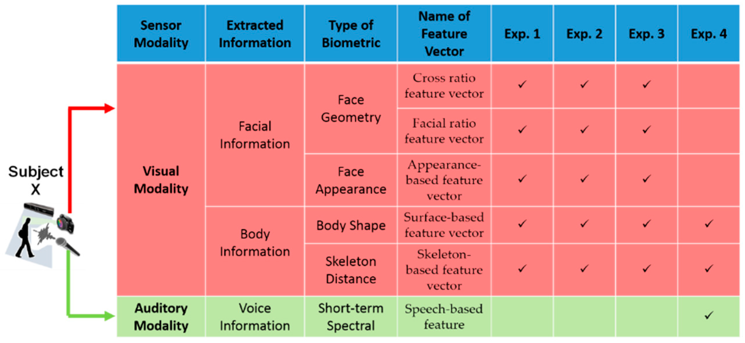
In this section, we present the experimental results to evaluate the performance of the person recognition algorithm in social settings. We have included four sets of simulation studies for person recognition to demonstrate the performance of the person recognition algorithm. The biometrics that have been extracted from visual and auditory modalities are presented in three groups, as shown in Figure 10. The biometrics that have been selected to identify a subject in each of the four scenarios are illustrated in Figure 10.
4.1. Generation of Multi-Modal Data Set
Our first challenge was that the available public datasets are generally unimodal, and as such, do not fit to the requirements of the multimodal perception. We resolved this problem by creating a new dataset from merging of the three datasets: FERET [57], TIDIGITS [58], and RGB-D [59]. FERET database contains a total of 14,126 facial images of 1199 individuals and 364 duplicate sets of facial images. TIDIGITS is a speech dataset that was originally collected at Texas Instruments Inc. (Dallas, TX, USA) The TIDIGITS corpus contain 326 speakers (111 men, 114 women, 50 boys and 51 girls), with each pronouncing 77 digit sequences. The RGB-D is a new database that was created by Barbosa et al. for the purpose of person re-identification studies based on information from 3D depth sensor. In this dataset, depth information has been obtained for 79 individuals with four scenarios: frontal view of person walking normally (Walking 1 group), frontal view of person walking slowly and avoiding obstacles (Walking 2 group), walking with stretched arms (Collaborative group), and back view of person walking normally (Backward group). Five synchronized information for each person namely, RGB images, foreground mask, skeleton, 3D mesh, and the estimated floor were collected in an indoor environment, whereby the individuals were at least two meters away from the 3D depth sensor.
In order to provide the individual in RGB-D database with facial images from a diverse group across ethnicity, gender, and age, we randomly selected 79 subjects from FERET database. Then, we used only frontal view images, which included frontal images at different facial expressions (fb image), different illuminations (fc image). Also, some subjects in the database wore glasses on and/or pull their hair back. The duplicate set contains frontal images of a person which was taken on a different day over one year, and for some individuals more than two years had elapsed between their first frontal images and the duplicate ones. The number of frontal facial images for each subject in the selected set varies from two to eight images. These 79 subjects were randomly assigned to subject in RGB-D database when considering that female subjects from FERET database are assigned to female subjects from RGB-D.
In order to complement the new dataset with speech data; we selected 23 subjects from women group in TIDIGITS dataset and assigned them randomly to female subjects in the new dataset, the rest of subjects in the new dataset were assigned with speech data from men group in TIDIGITS dataset.
The new dataset provides facial information, speech utterances, and the aforementioned information that is available on RGB-D database. The facial information is extracted from FERET database which provides facial frontal images with some differences such as changes in facial expression, change in illumination level, and variable amount of time between photography sessions. Also, RGB-D database provides skeleton and depth information that not affected by changing the outfits of the subjects and their bodies poses. On the other hand, TIDIGITS provide speaker signature when the subject is not in the field of view of robot’s vision system. It is important to note that the state-of-art face detection and recognition algorithms fail to provide quick detection and have low recognition rate when the face is angled or far from the camera, or when the face is partially occluded, and/or the illumination is poor. However, these situations are common in social HRI scenarios. In such cases, other biometrics features, such as body information and speech signature, can be used to compensate missing facial information and recognize an individual. These characteristics of the new database fit the requirements of the human-robot interactions in social settings where robust long-term interaction is a crucial factor for the success of the system.
The new (integrated) dataset has been partitioned into two sets, namely, training (gallery) and evaluation (probe) sets, as described in experiments 1 to 4. The gallery set was used to build the training model and the evaluation set was used for testing. The evaluation set is comprised of unseen data, not used in the development of the system. It is important to emphasize that the chronological order of the data capture was considered in constructing the evaluation set. Thus, some of the images in the evaluation set was chosen to be duplicate I and duplicate II, implying that they were taken at different dates, spanning from one day to two years. By using duplicate I and II images in constructing the evaluation sets, we ensured that the evaluation set represented closely scenarios that are appropriate for long-term HRI in social settings. The performance of the proposed architecture was evaluated in four experiments. Since, the data set has 79 subjects, thus the overall SNN was constructed from 79 circuits, as shown in Figure 8. In this SNN, all of the LIF neurons number 3 are connected laterally and all blocks have the same dendritic structure shown in Figure 8.
4.2. Experiment 1
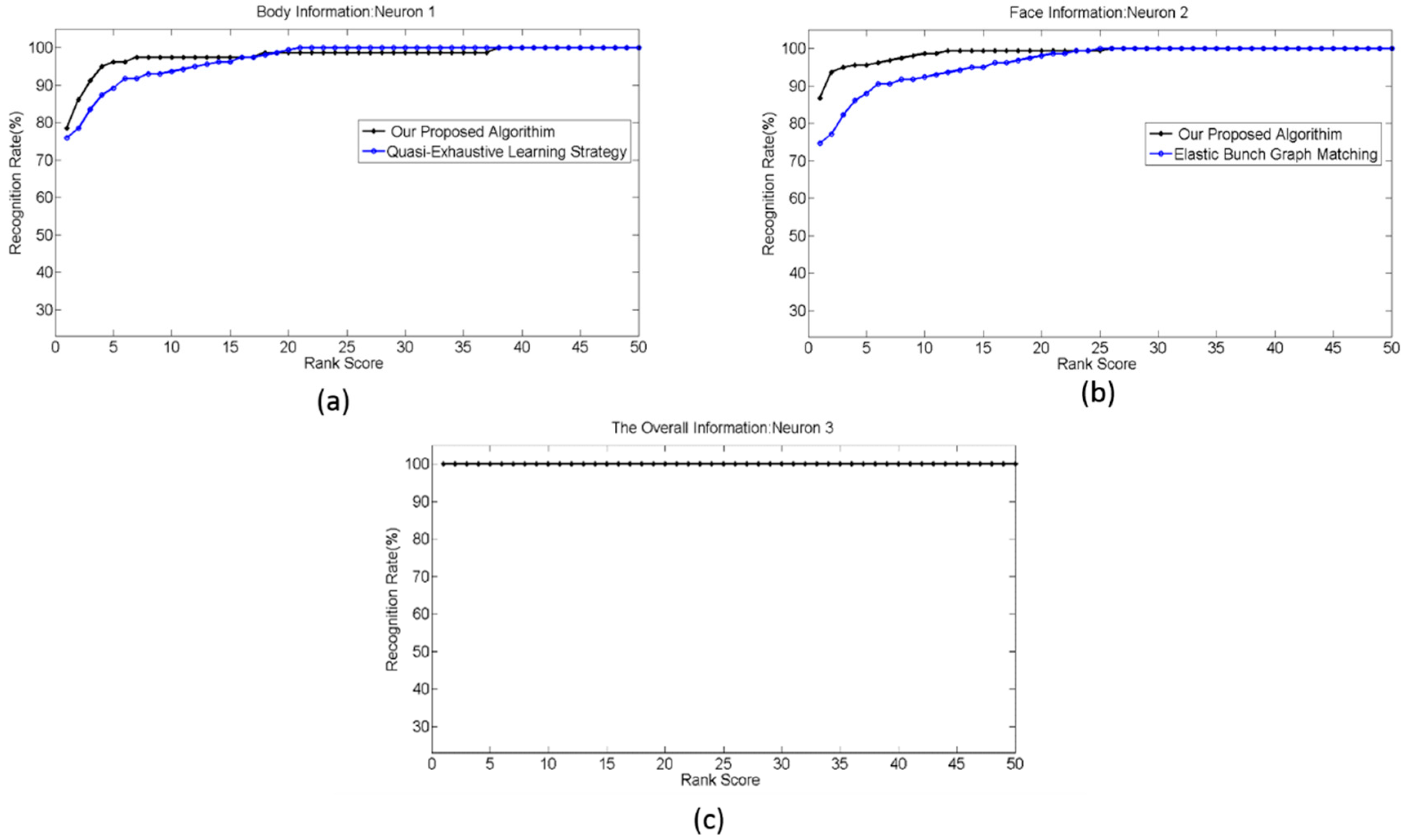
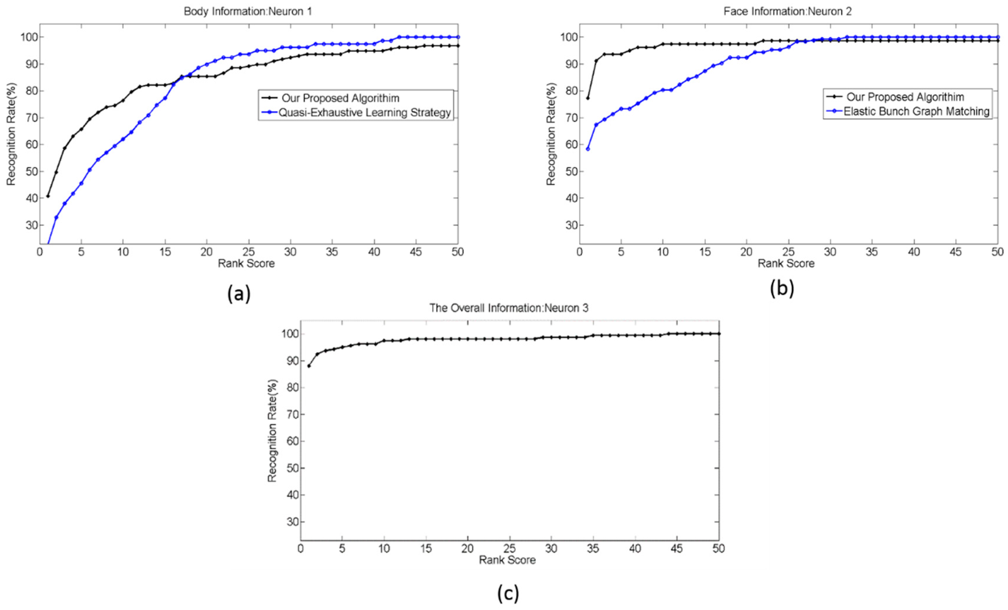
For each subject in the probe set, two facial images, fb image and its duplicate I image, were selected from the FERET database. In addition, two out of five frames from each of skeleton information and 3D mesh body information were selected randomly from Walking 1 group in the RGB-D database. The rest of the samples in the FERET and RGB-D databases were used to construct the training set. Some subjects in the FERET database had only two facial images. In this case, one was used for training and the other for evaluation. Five feature vectors were constructed, as described in Section 3. Three of the feature vectors represent facial information, including the facial geometry feature vector, cross ratio feature vector, and appearance-based feature vector. The rest of the feature vectors, namely the skeleton feature vector and the surface-based feature vector, represent the body information of the attended subject. IOs generated based on these features were converted into spike times and normalized to range from , prior to being fed to LIF neurons in SNN, as shown in Figure 8. The SNN was constructed and simulated using the neural Circuit (CSIM) simulator [60]. The parameters of LIF neurons were set as follows: the weight synapses of neuron 1 and neuron 2 were equal and set at . The weight synapses of neuron 3 were set as follows: the weight synapse of dendritic branch one was set to and weight synapse of dendritic branch two was set to , , , , , , , , , represents the input current supplied by the synapses, i.e., the outputs from the conversion process of IOs into input spike times. These input spike times were set in the range from . This selection is compatible with the natural human perception of time. The SNN were simulated for . As described in Section 2, the first neuron that fires a spike represents the best candidate of the attended subject from the gallery set. The overall SNN was constructed from 79 circuit blocks, as shown in Figure 8. Therefore, the total number of LIF neurons was 237. The recognition rates were calculated at two stages in the hierarchical structure of the SNN, namely stage 1 and stage 2. Stage 1 consists of the list of neurons, labeled as neuron 1 and neuron 2; stage 2 was represented by the list of neurons labeled as neuron 3. The recognition rate that was calculated from the list of neurons labeled as neuron 1 was based on body information; the recognition rates that were calculated from the list of neurons labeled as neuron 2 expressed a recognition rate based on facial information or voice information. Neuron 2 may use face geometry, face appearance, voice-based feature, or all of them in order to fire a spike. The same applies to neuron 1, which may use geodesic distances, skeleton distances, or both, in order to drive its potential to the threshold and consequently evoke a spike. The overall recognition rates were calculated based on neuron 3, which may use facial information, body information, voice information, or a combination of them. Cumulative match curves (CMCs) show the probability that the correct match of classification is found in the N, the most likely candidates, where N (the rank) is plotted on the x-axis. CMCs provide the performance measure for biometric recognition systems and have been shown to be equivalent to the ROC of the system [61]. The recognition result was averaged over ten runs; the cumulative match curves (CMCs) were plotted for these recognition results and are shown in Figure 11a–c.
4.3. Experiment 2
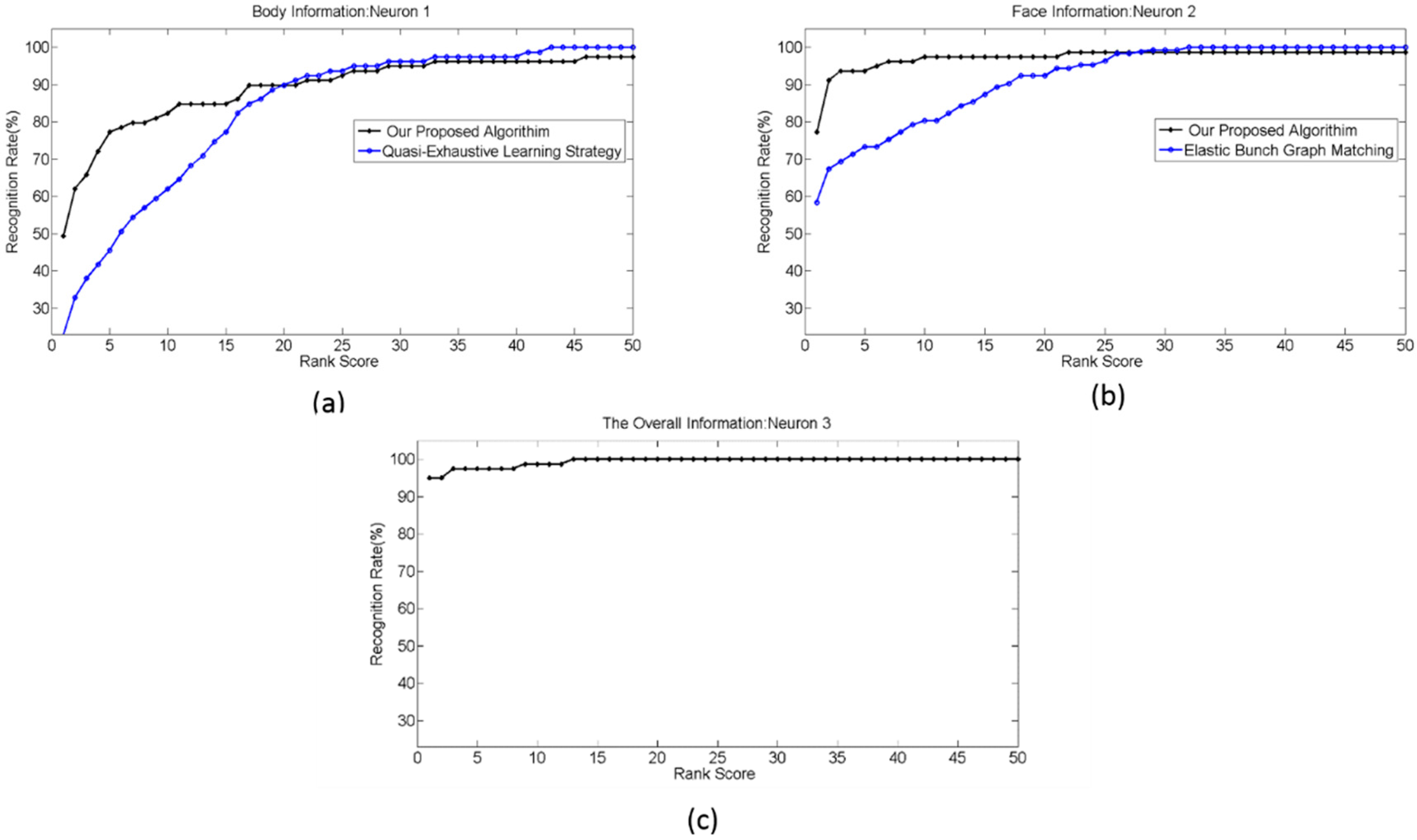
In this experiment, the probe set was constructed as follows: for body information, we used the collaborative group from the RGB-D database as the training set and two frames out of five from Walking 2 group as the probe set. For facial information, the probe set was constructed from fb image and duplicate II image. The rest of the samples in the FERET database was used to construct the training set. It can be noted that the probe and training sets were constructed in this manner to demonstrate the performance of the system in a real-world scenario where the enrolment process of the attended subject happened when the subject’s posture was different from that of the recognition process. All the other configurations of SNN were similar to the experiment 1. The recognition result was averaged over ten runs. The cumulative match curves (CMCs) were plotted for these recognition results and are shown in Figure 12a–c. The overall recognition rate is degraded as result of using different groups from the RGB-D database for training and evaluation. Hence, the same person is represented in one posture in gallery set and a different posture in the probe set. Another reason for the performance degradation is the use of the duplicate II image set to construct the probe set for the face information. This is a huge challenge for the state-of-the-art face recognition algorithms due to changes in illumination, aging, and facial expressions. Nevertheless, the proposed algorithm works reasonably well.
4.4. Experiment 3
We emulated a real-world scenario of HRI in social settings where biometric modalities that represent person identity are not concurrently available due to the sensor limitation or the occlusion of some parts of the person. To replicate this scenario, we converted the IOs generated from the body information into temporal spikes in range of 0–150 ms while the IOs that are generated from the face information were converted into temporal spikes in the range of 30–150 ms In this way, we made the body information available before the face information. This scenario replicates a situation where a person can be identified from his skeleton and body shape before face biometric modalities are available. Here, we assumed that the back view of the attended person is captured by the RGB-D sensor at the beginning of the recognition process and after a short time the attended person turned toward the camera in such a way that the face information becomes available. Hence, two frames out of five from the backward group in the RGB-D database are used to construct the probe set. For facial information, the probe set was constructed from fb image and duplicate II image, the same as in experiment 2. The rest of the samples in the FERET and RGB-D databases were used to construct the training set. All of the configurations of SNN are similar to the first experiment. The recognition result was averaged over ten runs, and the cumulative match curves (CMCs) were plotted for these recognition results, as shown in Figure 13a–c. The recognition rates are still good, despite the fact that biometric modalities are available at different times. We have not seen any other algorithm that copes with this scenario.
4.5. Experiment 4
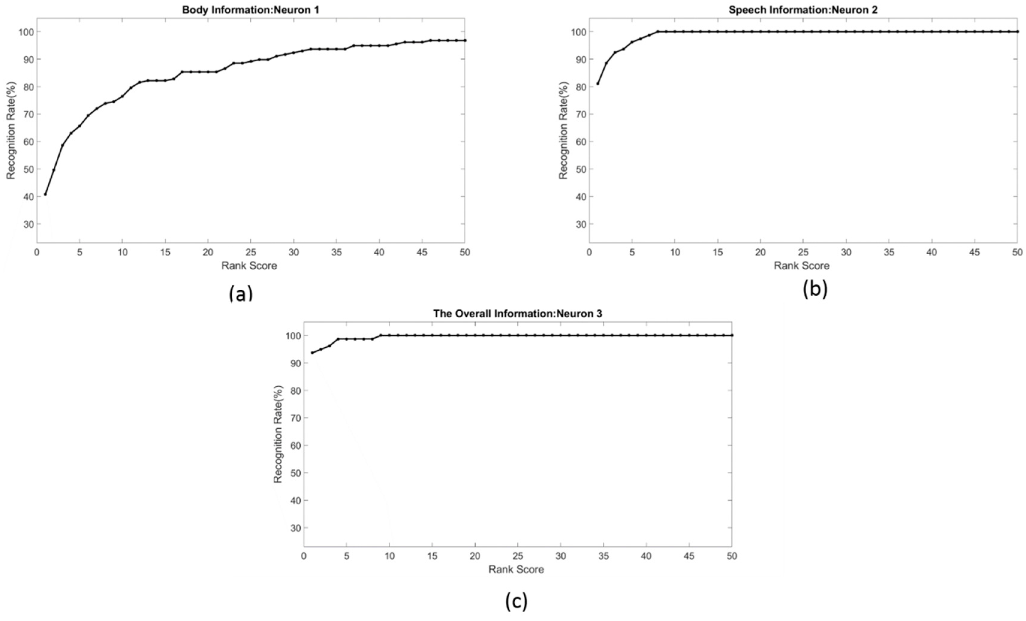
In this experiment, we emulated another challenging scenario of HRI in social settings when a subject’s face is not detected either due to distance between the robot and the subject or due to titled viewing angle of the camera and the head orientation. However, we assume that some utterances from subject’s speech can be captured by robot’s auditory system, as well as 3D mesh for subject’s body is available in robot’s vision stream of data. In this scenario, the subject’s speech signature and his/her body information are available. Here, we assumed that the audio signal is recorded first and the voice activity detector is applied such that only the voice signal is fed to speech feature extraction module. Also, we assumed that speech utterances of the attended person are captured by a microphone at the beginning of the recognition process, and after a short time, the attended person shows in camera’s view facing opposite way such that back view of body information becomes available. Thus, for each subject, two frames out of five from the backward group in the RGB-D database were used to construct the probe set for body information. The rest of the samples in the RGB-D database was used to construct the training set. For speech signature, the probe set was constructed by selecting seven utterances (each utterance in range of 1 to 1.7 s duration) out of 77 utterances from TIDIGITS database for each subject. The rest of the samples in the TIDIGITS database was used to construct the training set. Despite the fact that short speech utterances (such as the ones used in constructing the probe set for speech signature) reduce the recognition rate, we used them in our implementation to demonstrate its reasonable performance in this challenging HRI scenario. All of the configurations of SNN are similar to the first experiment. The recognition result was averaged over ten runs, and the cumulative match curves (CMCs) were plotted for these recognition results, as shown in Figure 14a–c. The recognition rates are still good, despite the fact that biometric modalities are available at different times and only two of them are available. We have not seen any other algorithm that copes with this scenario.
5. Discussions
In this section, we outline some design guidelines for the proposed system. The results suggest that the recognition rates using one modality or one source of information (i.e., recognition rate calculated at stage 1, represented by neuron 1 and neuron 2) are very close to other studies reported in literature which use similar modalities. However, when the outcomes of these modalities are represented as IOs and introduced to the temporal binding mechanism, the recognition rates dramatically improved. One key distinction of the proposed approach from other works is that it employs efficient processing of available information in multimodal sensors streams. The efficient processing is manifested by using a limited number of feature vectors and a limited number of elements in each vector in order to reduce the processing time of the feature vectors. For instance, the appearance-based feature vector can be constructed by applying the Gabor filter to the whole face, which may enhance the recognition rate, as calculated based on face information, and consequently increase the overall recognition performance of the system. However, the Gabor filter uses convolution operator which comes with a high computational cost. Hence, we applied the Gabor filter to selected fiducial points to reduce computational cost and exploit other biometric features in order to emphasize the real-time fashion of social human-robot interaction. The proposed approach exploits the fact that every modality participating in the encoding process of the attended subject possesses complementary information and has a discriminative level, which may be sufficient to independently identify a person and classify the individual to the correct class. In the case that the discriminative level of one modality is not sufficient to drive the system to the required threshold and finalize the identification process, it can be combined with other modalities at the intermediate level in a synergistic fashion to satisfy the required threshold, and consequently achieve higher performance.
One of the significant challenges of the person recognition tasks in social settings is that not all biometric modalities are available at the same time, due to a dynamic environment, human activities, and sensor limitations. Additionally, the nature of the HRI in social settings demands a perceptual system that is capable of providing a decision within the range of human response time; i.e., a human’s reaction time. For the above reasons, exploiting the available modalities and compromising between reliability of the outcomes and fast recognition are the main characteristics of the recognition system, making it appropriate for person recognition tasks in social settings. The results show that the system achieves high performance in real-time fashion, despite the fact that not all biometric modalities are available at the same time. Table 1 shows the results of other studies that use multimodalities for person recognition tasks. Most of the reported methods use biometric modalities that are essentially invasive and require close cooperation from the attended person. Only two methods, [18] and [8], may be classified as non-invasive multimodal biometric identification systems. One shortcoming of one of these two works [8] is that the overall recognition rate is limited by the detection rates of the modalities participating in encoding the attended person. In addition, most of the works that are reported in Table 1 use one main modality as the basis to extract other auxiliary features. These are normally referred to as soft biometric features, such as gender, ethnicity, and height, which in turn are fused together in order to improve the recognition rate. Another shortcoming of all of the works reported in Table 1, including the two non-invasive approaches, is that these systems assume all modalities are available at the same times. This requirement is not normally met in real-world HRI scenarios in social settings. Thus, the main shortcoming of these approaches is that the absence of the main modality leads to failure of the overall system.
6. Conclusions
We applied an elegant and a powerful multimodal perceptual system to address the problem of person recognition for social robots. The system can be used in a wide range of applications where a decision is expected based on the inputs from several sensors/modalities. The key distinction of this system from others is that it is non-invasive and does not require that all input stimuli are simultaneously available. The decision making process is facilitated by any modality that is rich in information and first becomes available. The system is also expected to make its decision within the same timeframe as humans (similar to duration for human response time).
In addition, the proposed system has the ability to adapt to real-world scenarios of social human-robot interactions by adjusting the threshold value which compromises between the reliability of the perception outcome and the time required to finalize the perception process. Going through the literature of person recognition systems, we note that there are almost no multimodal systems that are completely noninvasive, whereas the proposed system is noninvasive. We also note that a system that is based on “fusion” is conceptually and operationally different from the proposed architecture. The idea of fusion is to integrate the effect of several sensors with a view that each sensor by its own is not able to contribute to a correct decision; as such, the signals are fused together to enhance the decision making. The proposed system is designed based on the idea of convergence zone (as the term is used in neuroscience). This is further elaborated in Figure 1a,b. The modules “Conversion of IOs to spiking networks” and “Temporal binding” (Figure 1a) are analogous to “Multimodal Association Cortex”. The process is essentially different from “fusion”.
We have conducted extensive simulations and comparative studies to evaluate the performance of the proposed method. In order to generate a multimodal dataset, we combined the FERET, TIDIGITS, and RGB-D datasets to generate a new dataset that is applicable to multimodal systems. Simulation studies are promising and suggest notable advantages over related methods for person recognition.
Acknowledgments
This research was partially funded by NSERC and Simon Fraser University, respectively. The authors also acknowledge funds from Simon Fraser University for covering the costs to publish in open access.
Author Contributions
Mohammad Al-Qaderi is a PhD candidate undertaking his research under the supervision of Ahmad Rad.
Conflicts of Interest
The authors declare no conflict of interest.
Appendix A
L1Norm, L2 Norm, Mahalanobis distance, Cosine Similarity can be computed as (1) to (4) respectively.
where is a feature vector represents a subject in probe set, is a feature vector represents a subject in gallery set, is a covariance matrix.

Table A1.
Facial feature ratios.
A, B, C, D, E, F, G, H, I, J, K, L, Mc and N are the selected fiducial points on a face image, as shown in Figure 4a.
Appendix B
Table A2.
Euclidean distance of selected skeleton segments.
| (Skeleton-Based Feature) |
|---|
| • Euclidean distance between floor and head. • Euclidean distance between floor and neck. • Euclidean distance between floor and left hip. • Euclidean distance between floor and right hip. • Mean of Euclidean distances of floor to right hip and floor to left hip. • Euclidean distance between neck and left shoulder. • Euclidean distance between neck and right shoulder. • Mean of Euclidean distances of neck to left shoulder and neck to right shoulder. • Ratio between torso and legs. • Euclidean distance between torso and left shoulder. • Euclidean distance between torso and right shoulder. • Euclidean distance between torso and mid hip. • Euclidean distance between torso and neck. • Euclidean distance between left hip and left knee. • Euclidean distance between right hip and right knee. • Euclidean distance between left knee and left foot. • Euclidean distance between right knee and right foot. • Left leg length. • Right leg length. • Euclidean distance between left shoulder and left elbow. • Euclidean distance between right shoulder and right elbow. • Euclidean distance between left elbow and left hand. • Euclidean distance between right elbow and right hand.Left arm length. • Right arm length. • Torso length. • Height estimate. • Euclidean distance between hip center and right shoulder. • Euclidean distance between hip center and left shoulder. |
Table A3.
geodesic distances among the projection of selected skeleton joints.
| (Surface-Based Feature Vector) |
|---|
| • Geodesic distance between left hip and left knee. • Geodesic distance between right hip and right knee. • Geodesic distance between torso center and left shoulder. • Geodesic distance between torso center and right shoulder. • Geodesic distance between torso center and left hip. • Geodesic distance between torso center and right hip. • Geodesic distance between right shoulder and left shoulder. • Geodesic distance between left hip and left knee. • Geodesic distance between right hip and right knee. • Geodesic distance between torso center and left shoulder. • Geodesic distance between torso center and right shoulder. • Geodesic distance between torso center and left hip. • Geodesic distance between torso center and right hip. • Geodesic distance between right shoulder and left shoulder. |
References
- Chalabi, M. How Many People Can You Remember? 2015. Available online: https://fivethirtyeight.com/features/how-many-people-can-you-remember/ (accessed on 15 April 2016).
- Sacks, O.W. The Mind’s Eye, 1st ed.; Alfred A. Knopf: New York, NY, USA, 2010. [Google Scholar]
- Brunelli, R.; Falavigna, D. Person identification using multiple cues. IEEE Trans. Pattern Anal. Mach. Intell. 1995, 17, 955–966. [Google Scholar] [CrossRef]
- Zhou, X.; Bhanu, B. Feature fusion of side face and gait for video-based human identification. Pattern Recognit. 2008, 41, 778–795. [Google Scholar] [CrossRef]
- Zhou, X.; Bhanu, B. Integrating face and gait for human recognition at a distance in video. IEEE Trans. Syst. Man Cybern. Part B Cybern. 2007, 37, 1119–1137. [Google Scholar] [CrossRef]
- Palanivel, S.; Yegnanarayana, B. Multimodal person authentication using speech, face and visual speech. Comput. Vis. Image Underst. 2008, 109, 44–55. [Google Scholar] [CrossRef]
- Gong, S.; Cristani, M.; Yan, S.; Loy, C.C. (Eds.) Person Re-Identification; Springer: London, UK, 2014. [Google Scholar]
- Dantcheva, A.; Velardo, C.; D’Angelo, A.; Dugelay, J.-L. Bag of soft biometrics for person identification. Multimed. Tools Appl. 2011, 51, 739–777. [Google Scholar] [CrossRef]
- Arigbabu, O.A.; Ahmad, S.M.S.; Adnan, W.A.W.; Yussof, S. Recent advances in facial soft biometrics. Vis. Comput. 2015, 31, 513–525. [Google Scholar] [CrossRef]
- Feng, G.; Dong, K.; Hu, D.; Zhang, D. When Faces Are Combined with Palmprints: A Novel Biometric Fusion Strategy. In Biometric Authentication SE-95; Springer: Berlin/Heidelberg, Germany, 2004; Volume 3072, pp. 701–707. [Google Scholar]
- Jain, A.; Nandakumar, K.; Lu, X.; Park, U. Integrating faces, fingerprints, and soft biometric traits for user recognition. In Biometric Authentication; Springer: Berlin/Heidelberg, Germany, 2004; pp. 259–269. [Google Scholar]
- Raghavendra, R.; Dorizzi, B.; Rao, A.; Kumar, G.H. Designing efficient fusion schemes for multimodal biometric systems using face and palmprint. Pattern Recognit. 2011, 44, 1076–1088. [Google Scholar] [CrossRef]
- Samangooei, S.; Guo, B.; Nixon, M.S. The Use of Semantic Human Description as a Soft Biometric. In Proceedings of the 2nd IEEE International Conference on Biometrics: Theory, Applications and Systems, Arlington, VA, USA, 29 September–1 October 2008; pp. 1–7. [Google Scholar]
- Maity, S.; Abdel-Mottaleb, M.; Asfour, S.S. Multimodal Biometrics Recognition from Facial Video via Deep Learning. Signal Image Process. Int. J. 2017, 8, 81–90. [Google Scholar]
- Shahroudy, A.; Ng, T.-T.; Gong, Y.; Wang, G. Deep Multimodal Feature Analysis for Action Recognition in RGB+D Videos. IEEE Trans. Pattern Anal. Mach. Intell. 2016. [Google Scholar] [CrossRef] [PubMed]
- Frischholz, R.W.; Dieckmann, U. BiolD: A multimodal biometric identification system. Computer (Long Beach Calif.) 2000, 33, 64–68. [Google Scholar] [CrossRef]
- Ayodeji, O.; Mumtazah, S.; Ahmad, S.; Azizun, W.; Adnan, W. Integration of multiple soft biometrics for human identification. Pattern Recognit. Lett. 2015, 68, 278–287. [Google Scholar]
- Abreu, M.C.D.; Fairhurst, M. Enhancing Identity Prediction Using a Novel Approach to Combining Hard- and Soft-Biometric Information. IEEE Trans. Syst. Man Cybern. Part C (Appl. Rev.) 2011, 41, 599–607. [Google Scholar] [CrossRef]
- Dantcheva, A.; Elia, P.; Ross, A. What Else Does Your Biometric Data Reveal? A Survey on Soft Biometrics. IEEE Trans. Inform. Forensics Secur. 2016, 11, 441–467. [Google Scholar] [CrossRef]
- Liu, A.A.; Xu, N.; Nie, W.Z.; Su, Y.T.; Wong, Y.; Kankanhalli, M. Benchmarking a Multimodal and Multiview and Interactive Dataset for Human Action Recognition. IEEE Trans. Cybern. 2017, 47, 1781–1794. [Google Scholar] [CrossRef] [PubMed]
- Al-Hmouz, R.; Daqrouq, K.; Morfeq, A.; Pedrycz, W. Multimodal biometrics using multiple feature representations to speaker identification system. In Proceedings of the 2015 International Conference on Information and Communication Technology Research (ICTRC), Abu Dhabi, UAE, 17–19 May 2015; pp. 314–317. [Google Scholar]
- Karczmarek, P.; Kiersztyn, A.; Pedrycz, W. Generalized Choquet Integral for Face Recognition. Int. J. Fuzzy Syst. 2017, 1–9. [Google Scholar] [CrossRef]
- Boucenna, S.; Cohen, D.; Meltzoff, A.N.; Gaussier, P.; Chetouani, M. Robots Learn to Recognize Individuals from Imitative Encounters with People and Avatars. Sci. Rep. 2016, 6, 19908. [Google Scholar] [CrossRef] [PubMed]
- Asada, M.; Hosoda, K.; Kuniyoshi, Y.; Ishiguro, H.; Inui, T.; Yoshikawa, Y.; Ogino, M.; Yoshida, C. Cognitive Developmental Robotics: A Survey. IEEE Trans. Auton. Ment. Dev. 2009, 1, 12–34. [Google Scholar] [CrossRef]
- Clemo, H.R.; Keniston, L.P.; Meredith, M.A. Structural Basis of Multisensory Processing. In The Neural Bases of Multisensory Processes; CRC Press: Boca Raton, FL, USA, 2011; pp. 3–14. [Google Scholar]
- Stein, B.E. The New Handbook of Multisensory Processes; MIT Press: Cambridge, MA, USA, 2012. [Google Scholar]
- Romanski, L. Convergence of Auditory, Visual, and Somatosensory Information in Ventral Prefrontal Cortex. In The Neural Bases of Multisensory Processes; CRC Press: Boca Raton, FL, USA, 2011; pp. 667–682. [Google Scholar]
- Milner, A.D.; Goodale, M.A. The Visual Brain in Action, 2nd ed.; Oxford University Press: Oxford, NY, USA, 2006. [Google Scholar]
- Costanzo, L.S. Physiology, 2nd ed.; Saunders: Philadelphia, PA, USA, 2002. [Google Scholar]
- Halit, H.; de Haan, M.; Schyns, P.G.; Johnson, M.H. Is high-spatial frequency information used in the early stages of face detection? Brain Res. 2006, 1117, 154–161. [Google Scholar] [CrossRef] [PubMed]
- Goffaux, V.; Hault, B.; Michel, C.; Vuong, Q.C.; Rossion, B. The respective role of low and high spatial frequencies in supporting configural and featural processing of faces. Perception 2005, 34, 77–86. [Google Scholar] [CrossRef] [PubMed]
- Niculescu, A.; van Dijk, B.; Nijholt, A.; Limbu, D.K. Socializing with Olivia, the Youngest Robot Receptionist Outside the Lab. In International Conference on Social Robotics; Springer: Berlin/Heidelberg, Germany, 2010; pp. 50–62. [Google Scholar]
- Chellappa, R.; Wilson, C.L.; Sirohey, S. Human and machine recognition of faces: A survey. Proc. IEEE 1995, 83, 705–741. [Google Scholar] [CrossRef]
- Kauffmann, L.; Ramanoël, S.; Peyrin, C. The neural bases of spatial frequency processing during scene perception. Front. Integr. Neurosci. 2014, 8, 37. [Google Scholar] [CrossRef] [PubMed] [Green Version]
- Wallraven, C.; Schwaninger, A.; BÜlthoff, H.H. Learning from humans: Computational modeling of face recognition. Netw. Comput. Neural Syst. 2005, 16, 401–418. [Google Scholar] [CrossRef] [PubMed]
- Baltrusaitis, T.; Robinson, P.; Morency, L. OpenFace: An open source facial behavior analysis toolkit. In Proceedings of the 2016 IEEE Winter Conference on Applications of Computer Vision (WACV), Lake Placid, NY, USA, 7–10 March 2016. [Google Scholar]
- Rojas, M.M.; Masip, D.; Todorov, A.; Vitria, J. Automatic prediction of facial trait judgments: Appearance vs. structural models. PLoS ONE 2011, 6, e23323. [Google Scholar] [CrossRef] [PubMed]
- Tien, S.-C.; Chia, T.-L.; Lu, Y. Using cross-ratios to model curve data for aircraft recognition. Pattern Recognit. Lett. 2003, 24, 2047–2060. [Google Scholar] [CrossRef]
- Lei, G. Recognition of planar objects in 3-D space from single perspective views using cross ratio. IEEE Trans. Robot. Autom. 1990, 6, 432–437. [Google Scholar]
- Dijkstra, E.W. A note on two problems in connexion with graphs. Numerische Math. 1959, 1, 269–271. [Google Scholar] [CrossRef]
- Lowe, D.G. Object recognition from local scale-invariant features. In Proceedings of the Seventh IEEE International Conference on Computer Vision, Kerkyra, Greece, 20–27 September 1999; Volume 2, pp. 1150–1157. [Google Scholar]
- Bay, H.; Tuytelaars, T.; van Gool, L. Surf: Speeded up robust features. In Proceedings of the European Conference on Computer Vision, Graz, Austria, 7–13 May 2006; pp. 404–417. [Google Scholar]
- Shen, L.; Bai, L. A review on Gabor wavelets for face recognition. Pattern Anal. Appl. 2006, 9, 273–292. [Google Scholar] [CrossRef]
- Serrano, Á.; de Diego, I.M.; Conde, C.; Cabello, E. Analysis of variance of Gabor filter banks parameters for optimal face recognition. Pattern Recognit. Lett. 2011, 32, 1998–2008. [Google Scholar] [CrossRef]
- Sung, J.; Bang, S.-Y.; Choi, S. A Bayesian network classifier and hierarchical Gabor features for handwritten numeral recognition. Pattern Recognit. Lett. 2006, 27, 66–75. [Google Scholar] [CrossRef]
- Daugman, J.G. Two-dimensional spectral analysis of cortical receptive field profiles. Vis. Res. 1980, 20, 847–856. [Google Scholar] [CrossRef]
- Shen, L.; Bai, L. MutualBoost learning for selecting Gabor features for face recognition. Pattern Recognit. Lett. 2006, 27, 1758–1767. [Google Scholar] [CrossRef]
- Zheng, D.; Zhao, Y.; Wang, J. Features Extraction Using a Gabor Filter Family. In Proceedings of the Sixth Lasted International Conference, Signal and Image Processing, Honolulu, HI, USA, 23–25 August 2004; pp. 139–144. [Google Scholar]
- Serrano, Á.; de Diego, I.M.; Conde, C.; Cabello, E. Recent advances in face biometrics with Gabor wavelets: A review. Pattern Recognit. Lett. 2010, 31, 372–381. [Google Scholar] [CrossRef]
- Miller, G.A. The magical number seven, plus or minus two: Some limits on our capacity for processing information. Psychol. Rev. 1956, 63, 81–97. [Google Scholar] [CrossRef] [PubMed]
- Kinnunen, T.; Li, H. An overview of text-independent speaker recognition: From features to supervectors. Speech Commun. 2010, 52, 12–40. [Google Scholar] [CrossRef]
- Burkitt, A.N. A review of the integrate-and-fire neuron model: I. Homogeneous synaptic input. Biol. Cybern. 2006, 95, 1–19. [Google Scholar] [CrossRef] [PubMed]
- Branco, T.; Häusser, M. The single dendritic branch as a fundamental functional unit in the nervous system. Curr. Opin. Neurobiol. 2010, 20, 494–502. [Google Scholar] [CrossRef] [PubMed]
- London, M.; Häusser, M. Dendritic Computation. Annu. Rev. Neurosci. 2005, 28, 503–532. [Google Scholar] [CrossRef] [PubMed]
- Poirazi, P.; Brannon, T.; Mel, B.W. Pyramidal neuron as two-layer neural network. Neuron 2003, 37, 989–999. [Google Scholar] [CrossRef]
- Zhao, W.; Chellappa, R.; Phillips, P.J.; Rosenfeld, A. Face recognition: A literature survey. ACM Comput. Surv. 2003, 35, 399–458. [Google Scholar] [CrossRef]
- Phillips, P.J.; Rizvi, S.A.; Rauss, P.J. The FERET evaluation methodology for face-recognition algorithms. IEEE Trans. Pattern Anal. Mach. Intell. 2000, 22, 1090–1104. [Google Scholar] [CrossRef]
- Leonard, G.; Doddington, G. TIDIGITS LDC93S10. Web Download; Linguistic Data Consortium: Philadelphia, PA, USA, 1993. [Google Scholar]
- Barbosa, I.B.; Cristani, M.; del Bue, A.; Bazzani, L.; Murino, V. Re-identification with RGB-D sensors. In European Conference on Computer Vision; Springer: Berlin/Heidelberg, Germany, 2012; pp. 1–10. [Google Scholar]
- Maass, W.; Natschlager, T.; Markram, H. A model for real-time computation in generic neural microcircuits. In Proceedings of the Advances in Neural Information Processing Systems, Vancouver, BC, Canada, 9–14 December 2002; pp. 229–236. [Google Scholar]
- Bolle, R.M.; Connell, J.H.; Pankanti, S.; Ratha, N.K.; Senior, A.W. The relation between the ROC curve and the CMC. In Proceedings of the Fourth IEEE Workshop on Automatic Identification Advanced Technologies (AUTO ID 2005), Buffalo, NY, USA, 17–18 October 2005; Volume 2005, pp. 15–20. [Google Scholar]
- Jain, A.K.; Dass, S.C.; Nandakumar, K. Soft biometric traits for personal recognition systems. In Biometric Authentication; Springer: Berlin, Germany, 2004; pp. 731–738. [Google Scholar]
- Ailisto, H.; Vildjiounaite, E.; Lindholm, M.; Mäkelä, S.-M.; Peltola, J. Soft biometrics—Combining body weight and fat measurements with fingerprint biometrics. Pattern Recognit. Lett. 2006, 27, 325–334. [Google Scholar] [CrossRef]
- Zewail, R.; Elsafi, A.; Saeb, M.; Hamdy, N. Soft and hard biometrics fusion for improved identity verification. In Proceedings of the 2004 47th Midwest Symposium on Circuits and Systems, 2004 (MWSCAS ’04), Hiroshima, Japan, 25–28 July 2004; Volume 1, pp. 225–228. [Google Scholar]
Figure 1.
The proposed framework of brain-inspired multimodal perceptual system for social robots.

Figure 2.
Sophistication of the proposed framework for person recognition task in social settings. DPU: Dedicated Processing Unit; KNN: K-Nearest Neighbors; GMM: Gaussian Mixture Models.
Figure 2.
Sophistication of the proposed framework for person recognition task in social settings. DPU: Dedicated Processing Unit; KNN: K-Nearest Neighbors; GMM: Gaussian Mixture Models.

Figure 3.
The cross ratio relationship of two viewpoints.

Figure 4.
(a) Selected fiducial points on image from the FERET database which are used to construct the configural feature vector, (b) The cross ratio projection based on a polygon constructed from five fiducial points on face image from the FERET database.
Figure 4.
(a) Selected fiducial points on image from the FERET database which are used to construct the configural feature vector, (b) The cross ratio projection based on a polygon constructed from five fiducial points on face image from the FERET database.

Figure 5.
Selected skeleton joints, geodesic and Euclidean distance among them; (a) Projection of skeleton joints on the three-dimensional body point cloud, (b) Euclidian distance of selected skeleton segments, and (c) Sample of geodesic paths used in constructing surface-based feature vector.
Figure 5.
Selected skeleton joints, geodesic and Euclidean distance among them; (a) Projection of skeleton joints on the three-dimensional body point cloud, (b) Euclidian distance of selected skeleton segments, and (c) Sample of geodesic paths used in constructing surface-based feature vector.

Figure 6.
(a) Magnitude of Gabor filtered kernels at one scale {1}, two orientations {}, and three frequencies { }. (b) magnitude of Gabor filter responses on a sample image from the FERET database at one scale {1}, two orientations {}, and three frequencies { }.
Figure 6.
(a) Magnitude of Gabor filtered kernels at one scale {1}, two orientations {}, and three frequencies { }. (b) magnitude of Gabor filter responses on a sample image from the FERET database at one scale {1}, two orientations {}, and three frequencies { }.

Figure 7.
Modular representation of mel-frequency cepstral coefficients (MFCCs) feature extraction process.
Figure 7.
Modular representation of mel-frequency cepstral coefficients (MFCCs) feature extraction process.

Figure 8.
Spiking neural network (SNN) circuit and it dendritic structure that are used as a block to construct the overall SNN. LIF: leaky integrate-and-fire.
Figure 8.
Spiking neural network (SNN) circuit and it dendritic structure that are used as a block to construct the overall SNN. LIF: leaky integrate-and-fire.

Figure 9.
(a) The earliest spike is not sufficiently large to drive the neuron’s potential to threshold and evokes a spike, (b) The earliest spike is sufficiently large to drive the neuron’s potential to threshold and evokes a spike.
Figure 9.
(a) The earliest spike is not sufficiently large to drive the neuron’s potential to threshold and evokes a spike, (b) The earliest spike is sufficiently large to drive the neuron’s potential to threshold and evokes a spike.

Figure 10.
The Biometrics that have been discussed in the four experiments.

Figure 11.
(a) Cumulative match curves (CMC) based on body information calculated on Walking 1 group from the RGB-D database, (b) CMC based on face information calculated on fb and duplicate I images from the FERET database, and (c) CMC based on temporal binding of face and body information where body information is evaluated as described in Figure 11a and face information is evaluated as described in Figure 11b.

Figure 12.
(a) CMC based on body information calculated on Walking 2 group vs collaborative group from the RGB-D database, (b) CMC based on face information calculated on fb and duplicate II images from the FERET database, and (c) CMC based on temporal binding of face and body information where body information is evaluated as described in Figure 12a and face information is evaluated as described in Figure 12b.

Figure 13.
(a) CMC based on body information calculated on Backward group from the RGB-D database, (b) CMC based on face information calculated on fb and duplicate II images from the FERET database, (c) CMC based on temporal binding of face and body information where body information is evaluated as described in Figure 13a and face information is evaluated as described in Figure 13b.

Figure 14.
(a) CMC based on body information calculated on Backward group from the RGB-D database, (b) CMC based on speech information calculated on selected utterances from the TIDIGTS database, and (c) CMC based on temporal binding of speech and body information where body information is evaluated as described in Figure 14a and speech information is evaluated as described in Figure 14b.

Table 1.
Comparison with related works.
| Approach | Biometric Modalities | Category | Accuracy | No. of Subjects |
|---|---|---|---|---|
| [62] | fingerprint (main) + gender, ethnicity, and height (auxiliary) | invasive | 90.2% | 160 |
| [11] | face and fingerprint(main) + gender, ethnicity, and height (auxiliary) | invasive | 95.5% | 263 |
| [63] | fingerprint and body weight | invasive | 96.1% | 62 |
| [64] | fingerprint and iris | invasive | 97.0% | 21 |
| [18] | face (main) + age and gender (auxiliary) | non-invasive | 97.67% | 79 |
| [18] | fingerprint (main) + age and gender (auxiliary) | invasive | 96.76% | 79 |
| [8] | skin color, hair color, eye color, weight, torso clothes color, legs clothes color, beard presence, moustache presence, glasses presence | non-invasive | not available | 646 |
| our approach | face, body, speech, and skeleton | non-invasive | 100% (Figure 11c) | 79 |
© 2018 by the authors. Licensee MDPI, Basel, Switzerland. This article is an open access article distributed under the terms and conditions of the Creative Commons Attribution (CC BY) license (http://creativecommons.org/licenses/by/4.0/).
Share and Cite
MDPI and ACS Style
Al-Qaderi, M.K.; Rad, A.B. A Multi-Modal Person Recognition System for Social Robots. Appl. Sci. 2018, 8, 387. https://doi.org/10.3390/app8030387
AMA Style
Al-Qaderi MK, Rad AB. A Multi-Modal Person Recognition System for Social Robots. Applied Sciences. 2018; 8(3):387. https://doi.org/10.3390/app8030387
Chicago/Turabian StyleAl-Qaderi, Mohammad K., and Ahmad B. Rad. 2018. "A Multi-Modal Person Recognition System for Social Robots" Applied Sciences 8, no. 3: 387. https://doi.org/10.3390/app8030387
Note that from the first issue of 2016, this journal uses article numbers instead of page numbers. See further details here.