End-To-End Convolutional Neural Network Model for Gear Fault Diagnosis Based on Sound Signals
by
 , ,
, ,
Yong Yao
1, 
Honglei Wang
2,
Shaobo Li
1,3,*,
Zhonghao Liu
4,
Gui Gui
5,
Yabo Dan
1 and
Jianjun Hu
1,4,* 1
School of Mechanical Engineering, Guizhou University, Guiyang 550025, China
2
Guizhou Provincial Key Laboratory of Internet Collaborative Intelligent Manufacturing, Guizhou University, Guiyang 550025, China
3
Key Laboratory of Advanced Manufacturing Technology of Ministry of Education, Guizhou University, Guiyang 550025, China
4
Department of Computer Science and Engineering, University of South Carolina, Columbia, SC 29208, USA
5
National Institute of Measurement and Testing Technology, Chengdu 610021, China
*
Authors to whom correspondence should be addressed.
Appl. Sci. 2018, 8(9), 1584; https://doi.org/10.3390/app8091584
Submission received: 15 August 2018
/
Revised: 24 August 2018
/
Accepted: 30 August 2018
/
Published: 7 September 2018
(This article belongs to the Section Environmental Sciences)
Abstract
:Currently gear fault diagnosis is mainly based on vibration signals with a few studies on acoustic signal analysis. However, vibration signal acquisition is limited by its contact measuring while traditional acoustic-based gear fault diagnosis relies heavily on prior knowledge of signal processing techniques and diagnostic expertise. In this paper, a novel deep learning-based gear fault diagnosis method is proposed based on sound signal analysis. By establishing an end-to-end convolutional neural network (CNN), the time and frequency domain signals can be fed into the model as raw signals without feature engineering. Moreover, multi-channel information from different microphones can also be fused by CNN channels without using an extra fusion algorithm. Our experiment results show that our method achieved much better performance on gear fault diagnosis compared with other traditional gear fault diagnosis methods involving feature engineering. A publicly available sound signal dataset for gear fault diagnosis is also released and can be downloaded as instructed in the conclusion section.
1. Introduction
As a necessary component of most mechanical equipment, gears are widely used in the system of engineering machinery, aerospace, and ship vehicles for its advantage of power transmission. Due to the complex structure and poor working condition of the transmission system, gears can be easily damaged and cause the machine to break down, which contributes to the increased failure probability of whole system. Therefore, it is in urgent demand to seek effective gear fault diagnosis methods that can effectively detect and identify fault feature information of gears.
In the past decade, a vibration signal analysis method has become one of the most used and effective methods for gear fault pattern recognition and fault localization due to the abundant information and clear physical meaning in the mechanical vibration signal [1,2,3,4,5,6,7,8,9,10,11,12]. For example, Li et al. [1] proposed a method of planetary gear fault diagnosis via feature extraction based on multi-central frequencies and vibration signal frequency spectrum. Liu et al. [2] proposed a feature extraction and gear fault diagnosis method based on vibrational mode decomposition, singular value decomposition, and convolutional neural network (CNN). Kuai et al. [3] used the method of permutation entropy of Complete Ensemble Empirical Mode Decomposition with Adaptive Noise (CEEMDAN) Adaptive Neuro-fuzzy Inference System (ANFIS) to make gear fault diagnosis in a planetary gearbox. However, in many practical situations, the installation of vibration sensors is usually inconvenient due to constraints imposed by working conditions or even the equipment themselves. Moreover, vibration signals are not easy to be measured in high temperature, high humidity, high corrosion, and toxic and harmful environments, so the vibration signal analysis method for gear fault diagnosis is limited by its requirement of contacted measuring. Considering that, it is in urgent need to develop acoustic-based diagnosis (ABD) methods to overcome this disadvantage via non-contact measurements.
In recent years, a few studies have explored various acoustic-based fault diagnosis techniques [13,14,15]. AIDA et al. [16] compared the advantages and disadvantages of non-contact, air-coupled ultrasonic sensors and contact piezoelectric ultrasonic sensors in health monitoring of rotating machinery. Scanlon et al. [17] used non-contact microphone sensors to acquire acoustic signals of rotating machinery for predicting residual life. Hecke et al. [18] designed a new acoustic emission sensor technique to detect the fault mode of the bearing. With the development of array measurement technology, some researchers also applied this technology in acoustic-based diagnosis. By combining near-field acoustic holography (NAH) with spatial distribution feature extraction, W.B. Lu et al. [19,20,21] proposed a gearbox fault diagnosis method that is based on the spatial distribution features of a sound field. The NAH technology was used to reconstruct the sound field near the sound source, and then texture features were extracted from the acoustic images to reflect the distribution characteristics of the sound field. Finally, combining with the support vector machine-based pattern classification, the fault diagnosis of a gearbox was realized. Rong-Hua Hu et al. [22] proposed a rolling bearing fault diagnosis method, which is based on NAH and a grey-level gradient co-occurrence matrix (GLGCM). The NAH technology was also used to reconstruct sound files of different bearing conditions, then GLGCM features were extracted from the acoustic images and support vector machines were used for rolling bearing fault diagnosis. These methods overcame the limitations of traditional single channel measurement-based ABD methods and solved the local diagnosis problem in ABD.
Although all these sound signal based methods can work in fault diagnosis and have the capability to detect fault modes, they rely heavily on prior knowledge of signal processing techniques and diagnostic expertise, especially for the analysis of multiple channel measurement signals [23]. Deep learning models [24] can overcome this limitation. Pre-processed data can be directly fed as samples to train deep neural networks without manual feature extraction and selection. At present, deep learning models have been widely applied in speech recognition [25,26], acoustic scene classification [27,28], and environmental sound classification [29,30]. Many researchers also applied deep learning models in vibration signal analysis to detect fault modes [1,2,4,31]. However, there are few studies applying deep learning in ABD for two reasons: (1) the scarcity of publicly available acoustical signal fault diagnosis datasets like Case Western Reserve University bearing vibration signal datasets, and (2) acoustical signal acquisition requires a higher standard for environment and for equipment.
To address the obstacles as discussed above, a novel ABD method for gear fault pattern recognition is proposed. In our model, convolutional neural networks (CNN) are established to adaptively mine available fault characteristics by directly using time and frequency domain signals without other manually constructed features and automatically detect the fault modes of gears. In addition, we have released our acoustical gear fault diagnosis dataset to promote open research in the field of ABD. To our knowledge, this is the first such public sound dataset for gear fault diagnosis.
The main contributions of this paper are as follows:
- (1)
- Build and release the first ever publicly available sound dataset of gear fault diagnosis based on acoustical signal.
- (2)
- We designed an end-to-end stacked CNN model for an ABD task, which obtained information directly from time and frequency domain without feature engineering.
- (3)
- We are the first to use CNN instead of traditional fusion algorithms, such as Dempster-Shafer (D-S) evidence theory, to fuse multi-channel acoustical signals.
2. Model Building
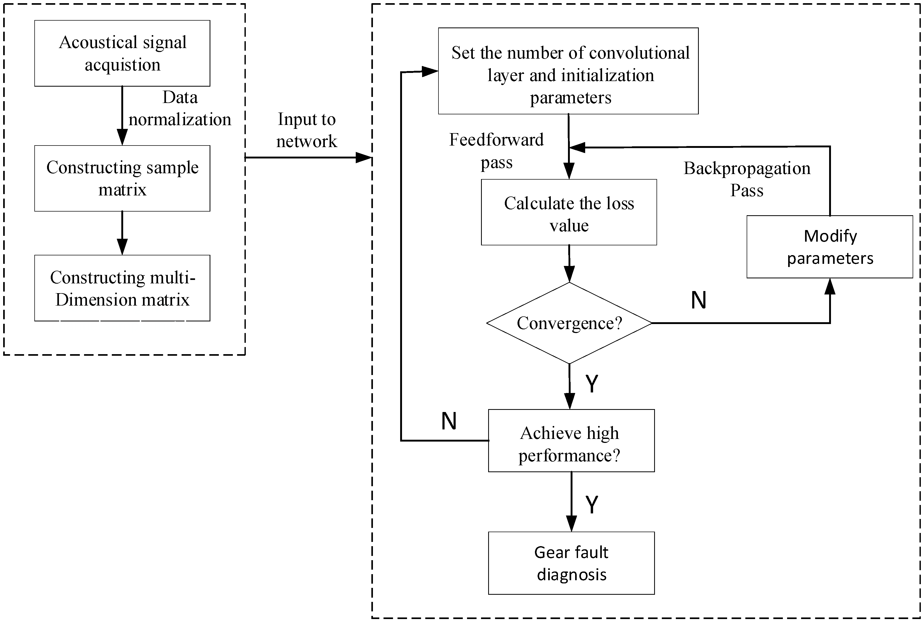
The mathematical model for our acoustic-based fault diagnosis method of gears can be roughly divided into three parts. In the first part, the time and frequency domain information are obtained from an original acoustical signal that are then combined into a sample matrix. The second part is to integrate multiple sample matrices, which are obtained from multi-channel acoustical sensors to become a multi-dimension matrix. In the last part, the multi-dimensional matrix is constructed as a CNN input to train the network. CNN is used to fuse multi-dimension information of the time and frequency domain and adaptively extract fault features and automatically identify fault patterns of gears to realize effective gears fault diagnosis. The block diagram of the proposed method is shown in Figure 1.
2.1. Information Acquisition in Time and Frequency Domain
As an automatic fault diagnosis method, our model does not rely on signal processing techniques and expertise of traditional feature extraction. We acquire the time domain information directly from original fault audio files generated from acoustic sensors installed around the gears and use sample matrix to represent it. The means the number of samples. indicates the time domain vector of sample , and represents the th time sequential parameter of the sample . Then, we apply a Fourier transform to each sample to obtain frequency domain signals. Transformed signals are added to the original time domain matrix as rows to construct a new matrix. The new matrix can be represented as followed:
It is composed of single channel signals in the time and frequency domain.
2.2. Multi-Channel Information Fusion
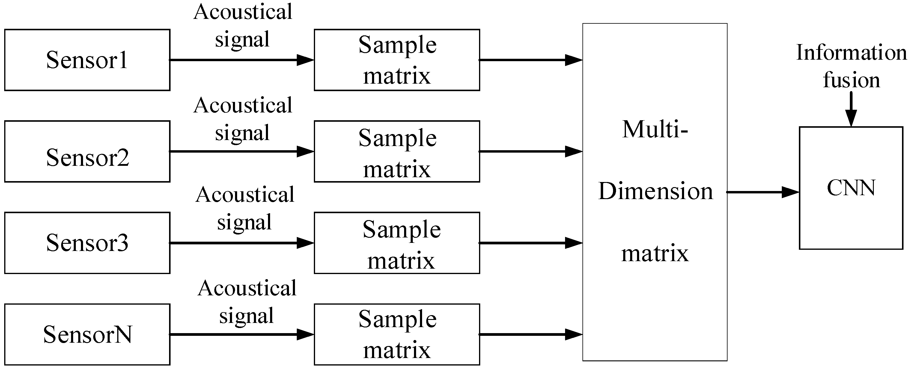
matrix contains fault information in the time and frequency domain of single channel acoustical signals about gears. We integrate multiple sample matrix to construct multi-dimension matrix . The represent sample matrix of the channel acoustical signals. The flowchart of the multi-channel information fusion method is shown in Figure 2.
These multi-dimensional matrices can be treated in quite a similar manner to the RGB input of an image in CNN. The convolutional neural network can be viewed as a fusion tool, which forms a more abstract high-level representation by combining the multi-channel information.
2.3. Fault Pattern Recognition Based on CNN
The end-to-end stacked CNN has the capability to establish the inner relationship between the time and frequency domain signals and fault types. The network consists of three functional layers: the convolutional layer, the batch normalization layer, and the fully connected layer.
The end-to-end convolutional layer can be viewed as a feature extraction representation jointly with classification to realize the adaptive feature extraction and feature identification. Convolution kernels are used to do convolution operations over multi-dimensional input matrices to extract different features and increase the bias to results. The equation is defined as followed:
where represents the feature map of layer , represents the output feature map of former layer, and represents the convolution operation between the output feature map of former layer and the feature map of layer . represents the input feature atlas and is a bias corresponding to .
The output feature of each convolutional layer is normalized by the batch normalization layer such that the mean and variance of the feature become 0 and 1 according to Equation (2).
where , represent the mean and variance of the mini-batch, respectively. However, the normalization processing between layers will change the distribution of data and learned features. Therefore, Equation (3) is used to restore the certain level features by transformation and reconstruction.
where , β are the two parameters that need to be learned, and the activation function is used to realize a nonlinear transformation for output features of each batch normalization layer.
Finally, the fault pattern recognition is realized by the fully connected layer. The calculation process of the fully connected layer can be expressed as follows:
where represents the input of the connected layer , represents the output of connected layer , and and represent weight and bias respectively.
2.4. Architecture and Parameter of End-To-End Stacked CNN Model
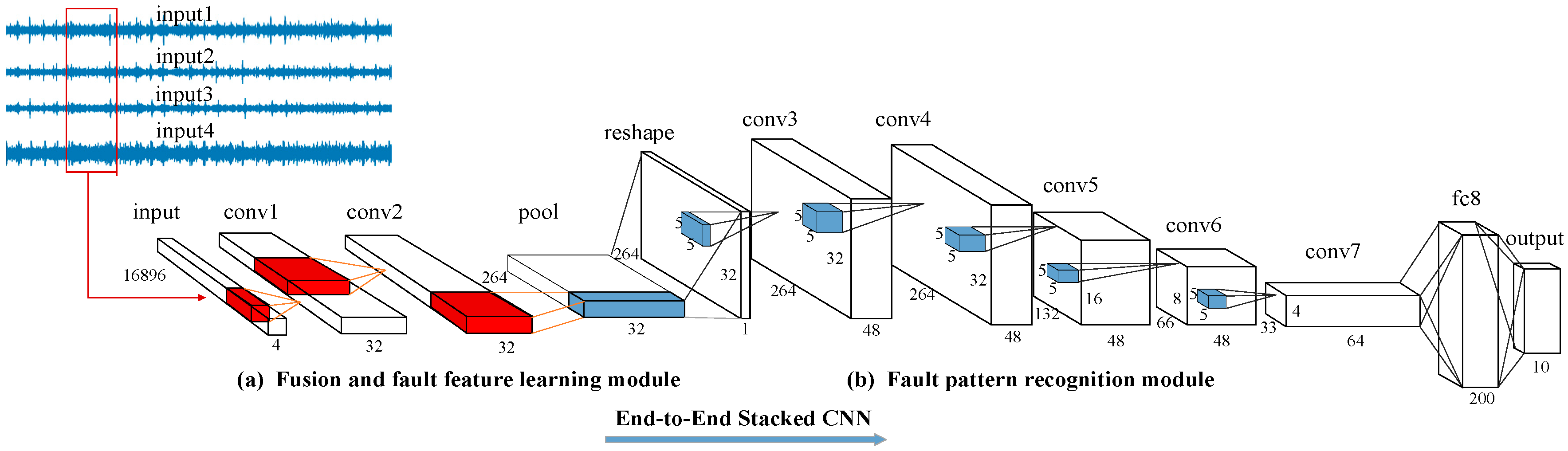
Our end-to-end stacked CNN model is shown in Figure 3.
The fusion and fault feature learning module contains two convolutional layers (before the pooling layer) to adaptively extract features from the sample matrices, which contains time and frequency domain signals with about 16,896 sampling points, with four channels. Each layer has 32 filters. The receptive field is set as (8,1) and the stride is set as (1,1) in both convolutional layers. This small filter size with two convolutional layers are set according to the experimental results of the Automatic speech recognition (ASR) task [25], which demonstrated that by using multi-convolutional layers with small receptive fields, the convolutional neural network model has the ability to extract local features of various scales hierarchically. The output of these two convolutional layers is noted as the “time–frequency” feature representation. After that, the non-overlapping maximum pooling with a 64 pooling size can be applied to the output of the convolutional layers. The output of the pool matrix has a size of (two-dimension feature matrix × channel). Then, the pool matrix is reshaped from to in order to convolve in both frequency and time. Finally, the three-dimensional matrix is used as input of “conv3” to achieve gear fault pattern classification.
The fault pattern recognition module contains five convolutional layers and one fully connected layer. The first two layers of module (b) uses 48 filters with a receptive field of (5,5) and stride of (1,1). The third and fourth layers have the same setting as the first two layers in the filters and receptive field, but the stride is set to (2,2). The last convolutional layer in module (b) uses 64 filters with a receptive field of (5,5) and stride of (2,2), and the hidden unit of fully connected layer is set to 200. In addition, the rectified linear unit (ReLU) is used as the activation function followed by each convolutional layer and fully connected layer. The output of the fully connected layer is followed by a softmax activation function. The detailed parameter of each layer is list in Table 1.
3. Experiment System
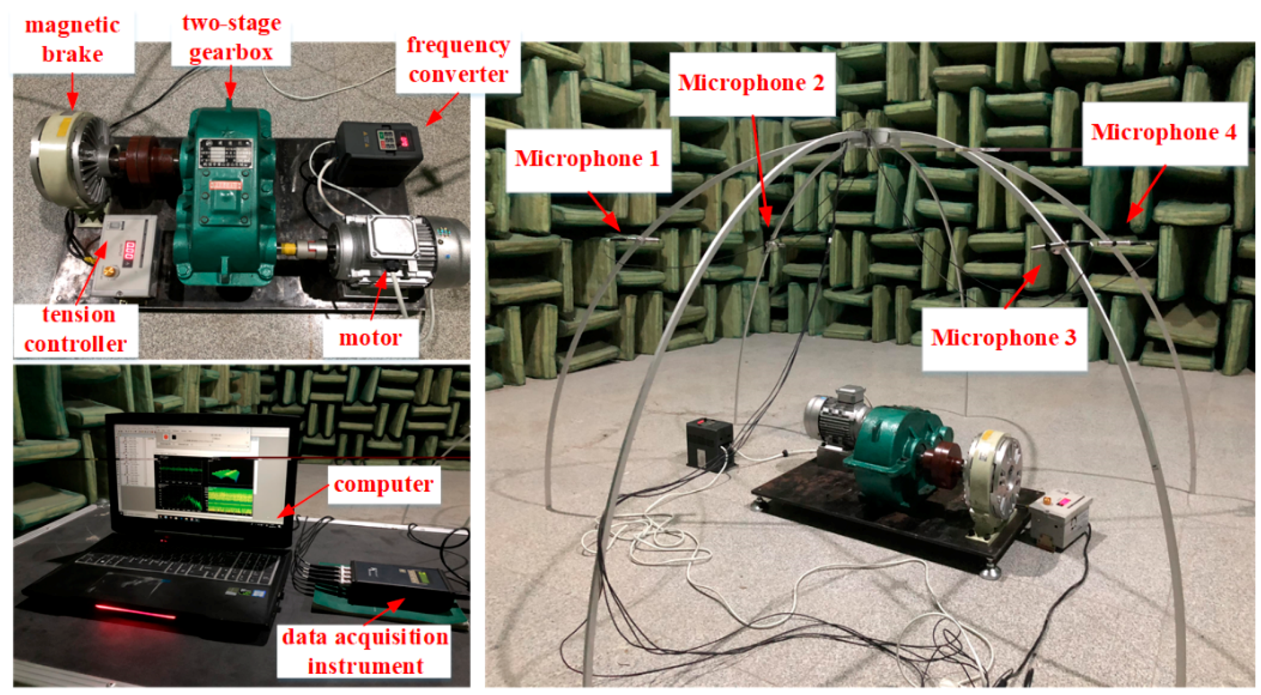
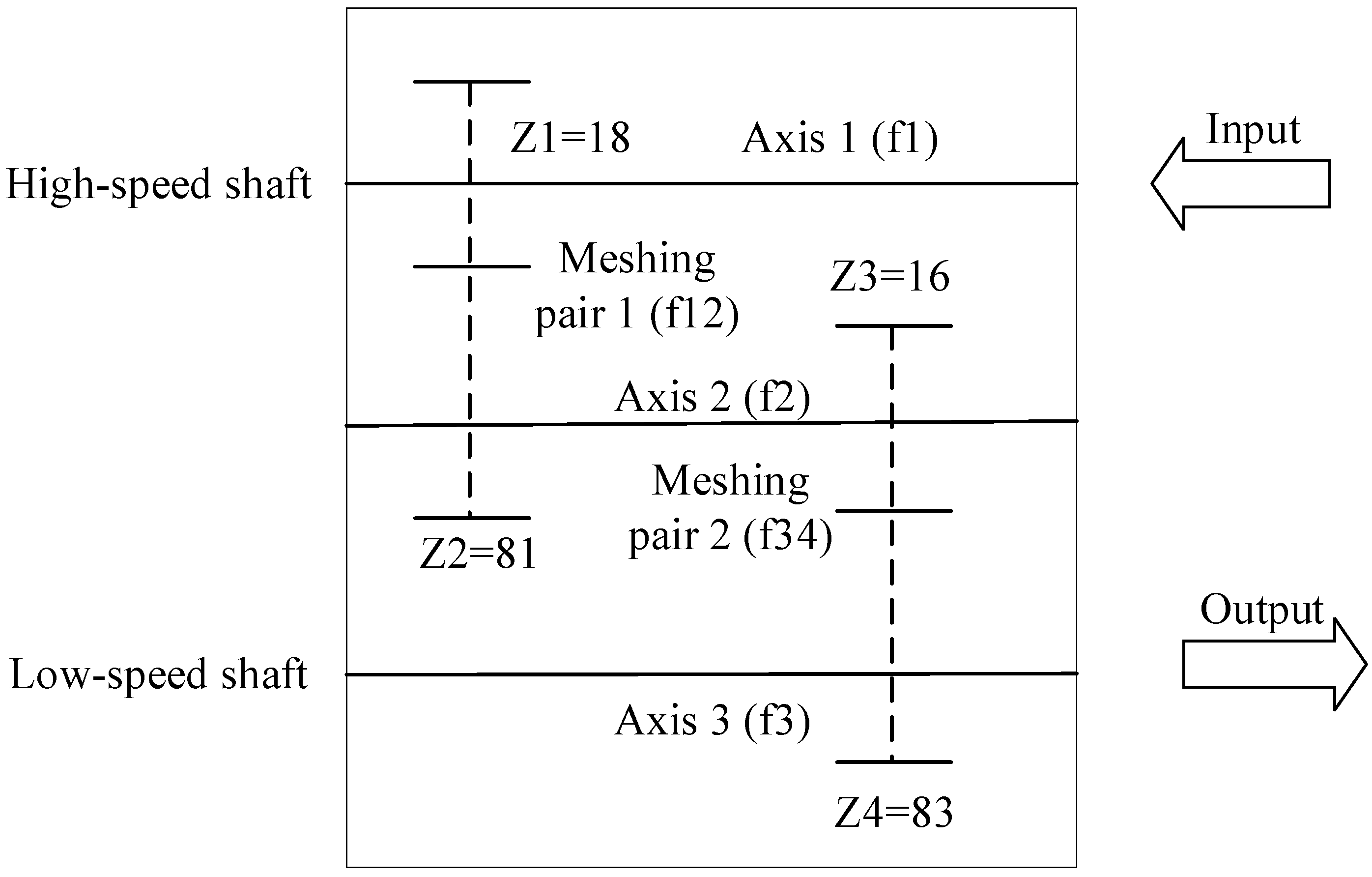
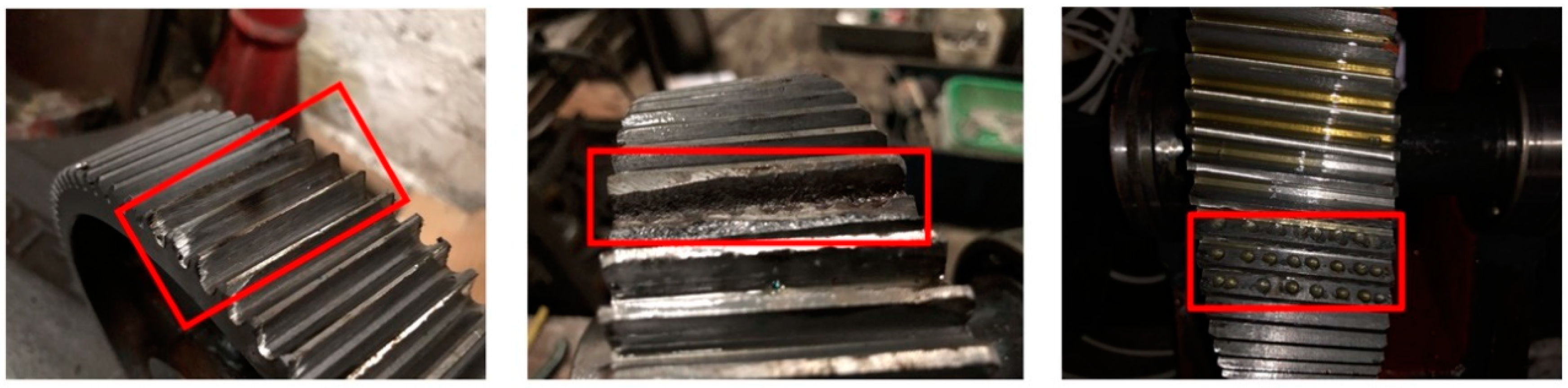
Gear fault diagnosis experiments based on an acoustical signal was conducted in a semi-anechoic room. The experiment system we built is composed of a two-stage gearbox, a variable frequency motor, a frequency converter, a programmable magnetic brake component, a tension controller, and measuring systems. The measuring system consisted of four 4189-A-021 free-field microphones from Denmark B&K company, a data acquisition instrument from Germany HEAD company, and Artemis data recording software. The microphones and data acquisition instrument were connected by a Bayonet Nut Connector (BNC) interface for data transmission and data were recorded by Artemis software. The whole experiment system is shown in Figure 4. The top-left corner of Figure 4 shows the test bench and the lower-left corner shows the data acquisition system. The two-stage gearbox reduction ratio was 23.34, the high-speed shaft reduction ratio was 18/81, and the low speed shaft reduction ratio was 16/83. The sketch map of the gearbox is shown in Figure 5. In this study, the gear fault of low speed shaft was chosen to be studied, and the acoustical signals are collected from normal gears, gears with a tooth fracture, gears with pitting, and gears with wear. All these gears’ acoustical signals were measured by a four-channel microphone array, which was arranged symmetrically with a hemispherical enveloping surface and the coordinates were set according to the ISO 3745:2003 standard. The layout of the array is shown in right picture of Figure 4. The different fault patterns are shown in Figure 6.
We set the speed of motor to 1800 rev/min by adjusting the frequency converter. In this condition, the shaft frequency of the three shafts and the meshing frequency of the two pairs of gears are shown in Table 2. We assumed that the interference of other parts of the gearbox, such as bearing and shaft by vibration, were minor. The acoustical signal that we measured can be viewed as only containing the gears. In addition, the tension controlled by a programmable magnetic brake component was set to 0 mA and 0.45 mA to simulate the no load state and the load state of 13.5 Nm. the sampling frequency of microphones was set to 16,000 Hz. The audio file was recorded for 60 s, and for each fault type of gears, we collected 40 audio samples with four channels.
4. Experiment Result and Analysis
4.1. Dataset
We have built two different datasets: A and B, representing the no load state and load state, respectively. Each dataset contained audio files of four types of gear faults and each type had a four-channel audio file with 60 s. We split an audio file into six segments and each segment lasted 10 s. Therefore, each dataset had 960 segments for four fault types. Each segment was divided into 1-s samples with no overlap. We follow this pattern because 1-s samples were found to be an optimal size for analysis based on empirical experiments in an audio process task. Then, 1-s samples were used as training and testing samples for our end-to-end stacked CNN model. In total, for dataset A, we obtained 9600 samples including 6000 training samples, 2400 validation samples, and 1200 testing samples. Similarly, we also got 6000 training samples, 2400 validation samples, and 1200 testing samples for dataset B.
4.2. Time and Frequency Analysis
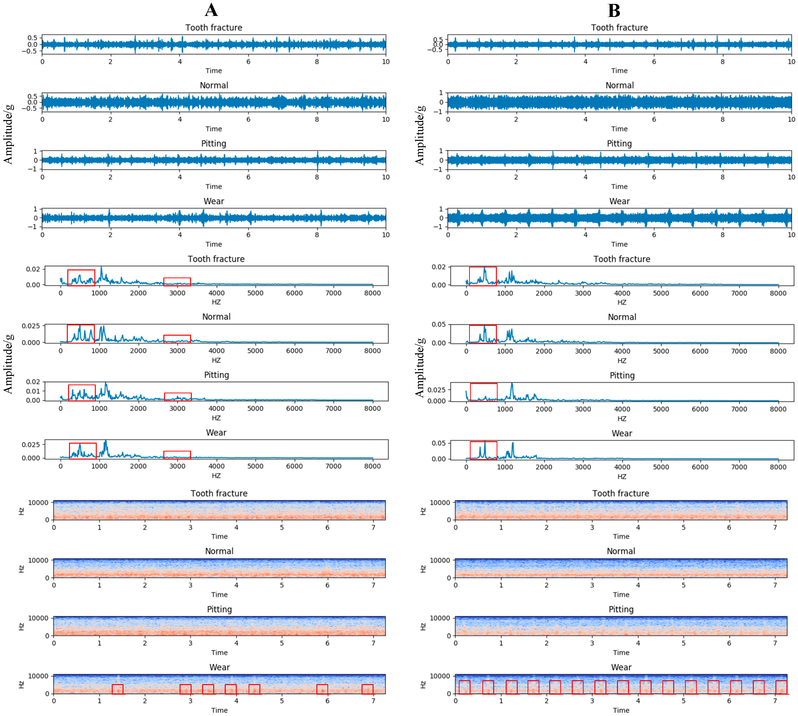
We took the gear of the gearbox’s low speed shaft as the research object. The acoustical signal collected from the normal gear, gear with tooth fracture, gear with pitting, and gear with wear under two different load conditions.
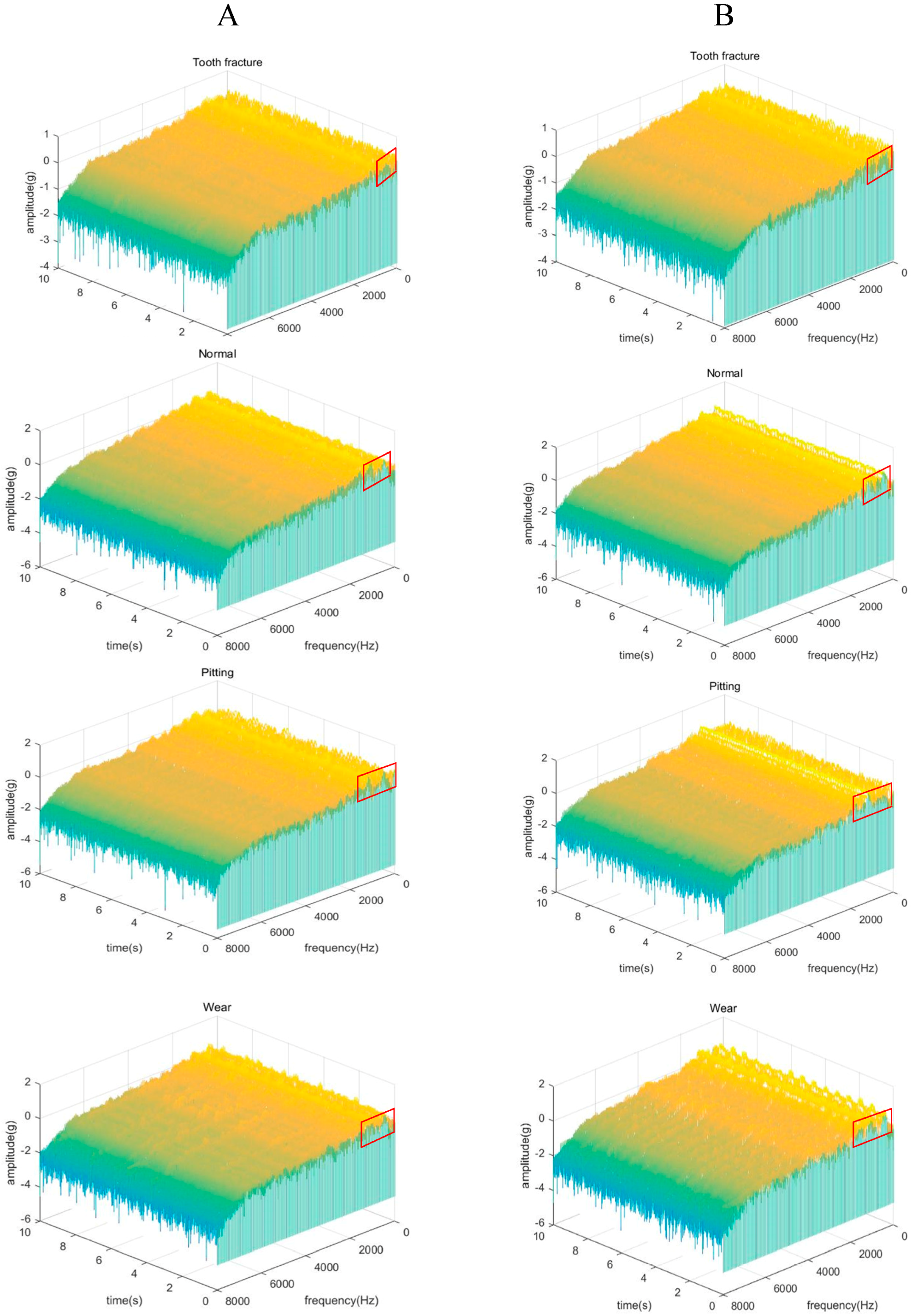
The left panel of Figure 7 shows the four types of gears in dataset A representing a no-load condition and the right panel shows the same type in dataset B representing a load condition. From the time domain signal, we can see that the waveform in three different types of gears, including tooth fracture, normal, and pitting, seemed to be obviously different in both datasets. The normal gears had a higher amplitude than the gears with a tooth fracture and the amplitude of pitting gears at certain time was 1 or −1, which was stronger than that of normal gears. This indicates that the time domain contained sufficient information to distinguish these three types of gears. As for the type of pitting and wear in gears, the differences were too subtle to be seen from the time domain signal. However, from the frequency domain signal, we found that the magnitude and distribution of the spectrum amplitude between different types of fault signals were different, especially in the range of 0 to 1000 Hz in dataset A and 0 to 800 Hz in dataset B, which meant the four different types of gears in a meshing condition had an obvious difference in meshing frequency. The types of pitting and wear in gears could be easily distinguished according to the magnitude of the spectrum amplitude in the range of 0–1000 Hz and 3000 Hz in dataset A and the range of 0 to 800 Hz in dataset B. The above conclusions were also shown in time–frequency domain. The above observation also holds in the time–frequency domain. From the spectrograms of Figure 7 and waterfall diagrams of Figure 8, we can see that the maximum amplitude of the four types of gears was in the range of 0–1000 Hz. The type of wear in gears had a stronger spectrum amplitude than the other three types of gears at certain time points in two datasets, which meant the type of wear in gears could be easily distinguished from the other three types of gears in the time–frequency domain. The above analysis shows that the acoustical signal in time and frequency domain contained sufficient information with four different types of gears. Therefore, we propose to integrate the time and frequency domain signals as a sample matrix to directly input into an end-to-end stacked convolutional neural network. Then, the end-to-end stacked CNNs were trained to adaptively mine available fault characteristics for fault diagnosis without manual feature engineering.
4.3. Multi-Channel Signal Analysis
The acoustical signals were acquired from four different microphones. Figure 9 shows the collected time and frequency domain signals of four different microphones in the gear fault of a tooth fracture with a no-load state.
It can be seen that the time domain waveforms of the fourth microphones were very different from other three microphones. The difference in acoustical signals from microphone 1 to microphone 3 could also be distinguished in frequency domain signals. From the right picture of Figure 9, we could find that the magnitude and distribution of the frequency amplitude between different microphones of fault signals were obviously different in the range of 0 to 1000 Hz. This indicates that each microphone obtained different acoustical signals because of the different acquisition positions. Therefore, in order to capture the entire acoustical signals of fault pattern, we needed to fuse multi-channel information that all these microphones collected. In this study, we first proposed to use CNN rather than a traditional fusion algorithm to fuse the multi-channel signals. This multi-channel information of time and frequency domains can be viewed similar to the RGB channels of images for pattern recognition using CNN.
4.4. Evaluation
End-to-end stacked CNN models were trained with the cross-entropy loss for multi-faulty type classification. An Adam optimization algorithm was employed as the training algorithm. The learning rate was 0.003. In addition, we used the early stopping approach to prevent overfitting and adopted the no-improvement-in-10-epochs strategy to identify the number of epochs via the validation set. Finally, our models adopted 70 and 50 of training epochs on datasets A and B, respectively.
In order to show the superiority of our method, we compared our model with traditional methods that combined manual features with conventional machine learning algorithms. The manual features that we extracted include a log-mel spectrogram, root-mean-square error (RMSE), and a spectral centroid. We combined these manual features as a matrix and fused multi-channel signals from four different microphones at the feature level. Four evaluation methods were designed to evaluate the generalization capability of the model:
In Evaluation 1, we trained a CNN model using the training samples from dataset A and tested it on the test samples in dataset A.
In Evaluation 2, we trained a CNN model using the training samples from dataset B and tested it on the test samples in dataset B.
In Evaluation 3, we trained a CNN model using the training samples from dataset A and tested it on the test samples in dataset B.
In Evaluation 4, we trained a CNN model using the training samples from dataset B and tested it on the test samples in dataset A.
We used the classification accuracy as the evaluation criterion, which is defined as , where represents the number of test samples recognized properly, and represents the total number of test samples.
The test results on two datasets are shown in Table 3.
From Table 3, we can see that the recognition accuracy of our end-to-end model reached 100% in Evaluation 1 and Evaluation 2 respectively. It was 1.2% and 1.4% higher than the accuracy of the best traditional method: manual features + SVM.
In order to further evaluate the generalization capability of our model, we added two more evaluation methods. The first method was training the model using the training samples in dataset A and testing it on test samples in dataset B. The second way was exchanging the training set and testing set in the first method. The reason why we adopted these evaluation methods was that a fault diagnosis algorithm with good generalization capabilities should still work even when the load condition changes. The test result showed that all methods decline in recognition accuracy, especially RandomForest and GBDT with manual features. The accuracy of RandomForest declined from 97.5% when evaluated on dataset A without load to 60.3% when tested on dataset B with a load with the same trained model. Similarly, the accuracy of GBDT declined from 95.7% when evaluated on dataset A without load to 58.9% when tested on dataset B with a load with the same trained model. Conversely, when we trained the RandomForest and GBDT models on dataset A without load and tested them on dataset B with a load, the prediction accuracy declines (from 93.6% to 87.7% for RandomForest; 96.5% to 93% for GBDT) were much smaller compared the previous cases. We suspect that some relationship between the feature spectrum and fault types exist in dataset B but not in dataset A so that training the model on dataset B and then testing it in dataset A can be viewed as some degree of overfitting to dataset B, which led to a low performance on test samples in dataset A. On the contrary, our model did not observe such a dramatic performance decline. In these two conditions, the accuracy of our model was 98.5% and 96.4% when trained on A and tested on B and when trained on B and tested on A. Both performances were higher than 95.2% of KNN with manual features and 94.5% SVM with manual features. The diagnosis result are shown in Table 4.
From the diagnosis result in Table 4, the recognition accuracy on gears with a tooth fracture reached 100% and 98.3% in Evaluation 3 and Evaluation 4, respectively, which meant these types of tooth fracture in gears could be easily distinguished from the other three types of gears. For normal gears, our algorithm achieved 99.0% accuracy in Evaluation 3 and 95.6% in Evaluation 4. The reason why the recognition accuracy decreased in Evaluation 4 is that the signal amplitude of the normal gears with a load and the amplitude of gears with pitting in the no-load state were similar at certain time points. As for the other two types of gears, the algorithm also achieved higher recognition accuracy in these two conditions. The reason for sample misclassifications here was due to the distribution of the amplitudes between these two types of fault signals, which were similar at certain times. This can be observed from time domain signal in Figure 7.
The above results indicate that our end-to-end stacked CNN model has achieved significant performance in sound signal-based gear fault diagnosis and has a strong generalization capability.
5. Conclusions
In this paper, we proposed a novel acoustic-based gear fault diagnosis method based on deep learning to recognize a fault pattern of gears. Using an end-to-end stacked CNN, the time and frequency domain signals could be directly input to the model without explicitly defining manual features as required by traditional fault diagnosis methods. The experiment results on two datasets showed that the accuracy of our model could reach 100% in the first two evaluation cases and 98.5%, 96.5% in the other two cases of evaluation respectively. All these performances were higher than those of other traditional fault diagnosis methods with manual features. This indicates that our model was more effective for fault diagnosis of gears with acoustical signals. Furthermore, to facilitate open research in the field of acoustic signal-based fault diagnosis, we publicly released the audio datasets of gears faults (https://mekhub.cn/yaoyong/gear_fault_all_dataset_sound), which contains four types of gear faults in a load state and a no-load state with 1800 rev/min. For the future study, we will continue to contribute more diverse audio datasets with different working and faulty conditions to further promote the research in ABD.
Author Contributions
Conceptualization, Y.Y., J.H., H.W. and S.L.; methodology, Y.Y.; software, Y.Y. and Y.D.; validation, Y.Y. and J.H.; investigation, Y.Y., H.W. and J.H.; resources, H.W. and S.L.; data curation, Y.Y. and G.G.; writing—original draft preparation, Y.Y. and J.H.; writing—review and editing, Y.Y., J.H. and Z.L.; supervision, S.L. and J.H.; project administration, H.W. and S.L.; funding acquisition, H.W. and W.L.
Funding
This research was funded by The National Natural Science Foundation of China under Grant No. 91746116 and 51741101, and Science and Technology Project of Guizhou Province under Grant Nos. supported this work. [2017]2308, Talents [2015]4011 and [2016]5013, Collaborative Innovation [2015]02.
Acknowledgments
We gratefully acknowledge the support of NVIDIA Corporation with the donation of the Titan X Pascal GPU used for this research and the support of National Institute of Measurement and Testing Technology with providing the semi-anechoic laboratory.
Conflicts of Interest
The authors declare no conflict of interest.
References
- Li, Y.; Cheng, G.; Pang, Y.; Kuai, M. Planetary Gear Fault Diagnosis via Feature Image Extraction Based on Multi Central Frequencies and Vibration Signal Frequency Spectrum. Sensors 2018, 18, 1735. [Google Scholar] [CrossRef] [PubMed]
- Liu, C.; Cheng, G.; Chen, X.; Pang, Y. Planetary Gears Feature Extraction and Fault Diagnosis Method Based on VMD and CNN. Sensors 2018, 18, 1523. [Google Scholar] [CrossRef] [PubMed]
- Kuai, M.; Cheng, G.; Pang, Y.; Li, Y. Research of Planetary Gear Fault Diagnosis Based on Permutation Entropy of CEEMDAN and ANFIS. Sensors 2018, 18, 782. [Google Scholar] [CrossRef] [PubMed]
- Li, S.; Liu, G.; Tang, X.; Lu, J.; Hu, J. An Ensemble Deep Convolutional Neural Network Model with Improved D-S Evidence Fusion for Bearing Fault Diagnosis. Sensors 2017, 17, 1729. [Google Scholar] [CrossRef] [PubMed]
- Yao, X.; Li, S.; Hu, J. Improving Rolling Bearing Fault Diagnosis by DS Evidence Theory Based Fusion Model. J. Sens. 2017, 1, 1–14. [Google Scholar] [CrossRef]
- Zhang, C.; Peng, Z.; Chen, S.; Li, Z.; Wang, J. A gearbox fault diagnosis method based on frequency-modulated empirical mode decomposition and support vector machine. Proc. Inst. Mech. Eng. C-J. Mech. Eng. Sci. 2016, 232, 369–380. [Google Scholar] [CrossRef]
- Sawalhi, N.; Randall, R.B. Vibration response of spalled rolling element bearings: Observations, simulations and signal processing techniques to track the spall size. Mech. Syst. Signal Process. 2011, 25, 846–870. [Google Scholar] [CrossRef]
- Sawalhi, N.; Randall, R.B. Gear parameter identification in a wind turbine gearbox using vibration signals. Mech. Syst. Signal Process. 2014, 42, 368–376. [Google Scholar] [CrossRef]
- Figlus, T.; Stańczyk, M. Diagnosis of the wear of gears in the gearbox using the wavelet packet transform. Metalurgija 2014, 53, 673–676. [Google Scholar]
- Borghesani, P.; Pennacchi, P.; Randall, R.B.; Sawalhi, N.; Ricci, R. Application of cepstrum pre-whitening for the diagnosis of bearing faults under variable speed conditions. Mech. Syst. Signal Process. 2013, 36, 370–384. [Google Scholar] [CrossRef]
- Abboud, D.; Antoni, J.; Eltabach, M.; Sieg-Zieba, S. Angle time cyclostationarity for the analysis of rolling element bearing vibrations. Measurement 2015, 75, 29–39. [Google Scholar] [CrossRef]
- Figlus, T.; Stańczyk, M. A method for detecting damage to rolling bearings in toothed gears of processing lines. Metalurgija 2016, 55, 75–78. [Google Scholar]
- Prainetr, S.; Wangnippanto, S.; Tunyasirut, S. Detection mechanical fault of induction motor using harmonic current and sound acoustic. In Proceedings of the 2017 International Electrical Engineering Congress (iEECON), Pattaya, Thailand, 8–10 March 2017. [Google Scholar]
- Glowacz, A. Acoustic based fault diagnosis of three-phase induction motor. Appl. Acoust. 2018, 137, 82–89. [Google Scholar] [CrossRef]
- Józwik, J.; Wac-Włodarczyk, A.; Michałowska, J.; Kłoczko, M. Monitoring of the Noise Emitted by Machine Tools in Industrial Conditions. J. Ecol. Eng. 2018, 19, 83–93. [Google Scholar] [CrossRef] [Green Version]
- Rezaei, A.; Dadouche, A.; Wickramasinghe, V.; Dmochowski, W. A comparison study between acoustic sensors for bearing fault detection under different speed and load using a variety of signal processing techniques. Tribol. Trans. 2011, 54, 179–186. [Google Scholar] [CrossRef]
- Scanlon, P.; Kavanagh, D.F.; Boland, F.M. Residual Life Prediction of Rotating Machines Using Acoustic Noise Signals. IEEE Trans. Instrum. Meas. 2012, 62, 95–108. [Google Scholar] [CrossRef]
- Hecke, B.V.; Qu, Y.; He, D. Bearing fault diagnosis based on a new acoustic emission sensor technique. J. Risk Reliab. 2015, 229, 105–118. [Google Scholar]
- Hou, J.; Jiang, W.; Lu, W. The application of NAH-based fault diagnosis method based on blocking feature extraction in coherent fault conditions. J. Vib. Eng. 2011, 24, 555–561. [Google Scholar]
- Hou, J.; Jiang, W.; Lu, W. Application of a near-field acoustic holography-based diagnosis technique in gearbox fault diagnosis. J. Vib. Control. 2011, 19, 3–13. [Google Scholar] [CrossRef]
- Lu, W.; Jiang, W.; Zhang, Y.; Zhang, W. Gearbox fault diagnosis based on spatial distribution features of sound field. J. Vib. Shock 2013, 32, 183–188. [Google Scholar]
- Hu, R.; Lu, W.; Zhang, Y. Rolling Element Bearing Fault Diagnosis Based on Near-field Acoustic Holography. Noise Vib. Control 2013, 3, 218–221. [Google Scholar]
- Lu, W. Diagnosing rolling bearing faults using spatial distribution features of sound field. J. Mech. Eng. 2012, 48, 68. [Google Scholar] [CrossRef]
- Hinton, G.E.; Salakhutdinov, R.R. Reducing the dimensionality of data with neural networks. Science 2006, 313, 504–507. [Google Scholar] [CrossRef] [PubMed]
- Hoshen, Y.; Weiss, R.J.; Wilson, K.W. Speech acoustic modeling from raw multichannel waveforms. In Proceedings of the 2015 IEEE International Conference on Acoustics, Speech and Signal Processing (ICASSP), Brisbane, Australia, 19–24 April 2015. [Google Scholar]
- Dai, W.; Dai, C.; Qu, S. Very deep convolutional neural networks for raw waveforms. In Proceedings of the 2017 IEEE International Conference on Acoustics, Speech and Signal Processing (ICASSP), New Orleans, LA, USA, 5–9 March 2017. [Google Scholar]
- Valenti, M.; Squartini, S.; Diment, A.; Parascandolo, G.; Virtanen, T. A convolutional neural network approach for acoustic scene classification. In Proceedings of the 2017 International Joint Conference on Neural Networks (IJCNN), Anchorage, AK, USA, 14–19 May 2017. [Google Scholar]
- Acoustic Scene Classification Using Convolutional Neural Network and Multiple-Width Frequency-Delta Data Augmentation. Available online: http://cn.arxiv.org/abs/1607.02383 (accessed on 15 August 2018).
- Piczak, K.J. Environmental sound classification with convolutional neural networks. In Proceedings of the 2015 IEEE 25th International Workshop on Machine Learning for Signal Processing (MLSP), Boston, MA, USA, 17–20 September 2015. [Google Scholar]
- Tokozume, Y.; Harada, T. Learning environmental sounds with end-to-end convolutional neural network. In Proceedings of the 2017 IEEE International Conference on Acoustics, Speech and Signal Processing (ICASSP), New Orleans, LA, USA, 5–9 March 2017. [Google Scholar]
- Guo, X.; Shen, C.; Chen, L. Deep Fault Recognizer: An Integrated Model to Denoise and Extract Features for Fault Diagnosis in Rotating Machinery. Appl. Sci. 2016, 7, 41. [Google Scholar] [CrossRef]
Figure 1.
Block diagram of the proposed method.

Figure 2.
Multi-channel information fusion flowchart.

Figure 3.
Architecture of the end-to-end stacked CNN. It consists of two parts: fusion and fault feature learning module (a) and fault pattern recognition module (b).
Figure 3.
Architecture of the end-to-end stacked CNN. It consists of two parts: fusion and fault feature learning module (a) and fault pattern recognition module (b).

Figure 4.
Experiment system in semi-anechoic.

Figure 5.
The sketch map of two-stage gearbox.

Figure 6.
Three different fault patterns of gears.

Figure 7.
Four different types of gear signals in time, frequency, and time–frequency domains under two-load conditions. (A) Represents a no-load condition and (B) represents a load condition.
Figure 7.
Four different types of gear signals in time, frequency, and time–frequency domains under two-load conditions. (A) Represents a no-load condition and (B) represents a load condition.

Figure 8.
Waterfall diagrams of four different types of gears under two-load conditions. (A) Represents a no-load condition and (B) represents a load condition.
Figure 8.
Waterfall diagrams of four different types of gears under two-load conditions. (A) Represents a no-load condition and (B) represents a load condition.

Figure 9.
Time and frequency domain signal from four microphones.


Table 1.
Parameter of the end-to-end stacked CNN.
| Layer | Input Shape | Filter | Kernel Size | Stride | Output Shape |
|---|---|---|---|---|---|
| Conv1 | [batch,16896,1,4] | 32 | (8,1) | (1,1) | [batch,16896,1,32] |
| Conv2 | [batch,16896,1,32] | 32 | (8,1) | (1,1) | [batch,16896,1,32] |
| Pool | [batch,16896,1,32] | - | (64,1) | (64,1) | [batch,264,1,32] |
| Reshape | [batch,264,1,32] | - | - | - | [batch,264,32,1] |
| Conv3 | [batch,264,32,1] | 48 | (5,5) | (1,1) | [batch,264,32,48] |
| Conv4 | [batch,264,32,48] | 48 | (5,5) | (1,1) | [batch,264,32,48] |
| Conv5 | [batch, 264,32,48] | 48 | (5,5) | (2,2) | [batch,132,16,48] |
| Conv6 | [batch,132,16,48] | 48 | (5,5) | (2,2) | [batch,66,8,48] |
| Conv7 | [batch,66,8,64] | 64 | (5,5) | (2,2) | [batch,33,4,64] |
| Fc8 | [batch,200] | - | - | - | [batch,4] |
Table 2.
Working frequency of each part of gearbox.
| Number | f1 | f12 | f2 | f34 | f3 |
| Working Frequency (Hz) | 25 | 540 | 15 | 106.6 | 3 |
Table 3.
The prediction accuracy on dataset A (without load) and dataset B (with load).
| Methods | Accuracy (%) on | |||
|---|---|---|---|---|
| Evaluation 1 Train on A Test on A | Evaluation 2 Train on B Test on B | Evaluation 3 Train on A Test on B | Evaluation 4 Train on B Test on A | |
| end-to-end (our method) | 100 | 100 | 98.5 | 96.4 |
| manual feature + SVM | 98.8 | 98.6 | 94.7 | 94.5 |
| manual feature + RandomForest | 93.6 | 97.5 | 87.7 | 60.3 |
| manual feature + GBDT | 96.5 | 95.7 | 93.0 | 58.9 |
| manual feature + KNN | 98.6 | 98.0 | 95.2 | 94.4 |
Table 4.
Diagnosis result of our method in Evaluation 3 and Evaluation 4.
| Method | Type | Diagnosis Result in Evaluation 3 | Accuracy (%) | ||||
|---|---|---|---|---|---|---|---|
| Sample | Tooth Fracture | Normal | Pitting | Wear | |||
| end-to-end (our method) | Tooth fracture | 300 | 300 | 0 | 0 | 0 | 100 |
| Normal | 300 | 0 | 297 | 1 | 2 | 99.0 | |
| Pitting | 300 | 1 | 1 | 293 | 5 | 97.6 | |
| Wear | 300 | 2 | 0 | 8 | 292 | 97.3 | |
| Type | Diagnosis Result in Evaluation 4 | Accuracy (%) | |||||
| Sample | Tooth Fracture | Normal | Pitting | Wear | |||
| Tooth fracture | 300 | 295 | 0 | 3 | 2 | 98.3 | |
| Normal | 300 | 0 | 287 | 9 | 4 | 95.6 | |
| Pitting | 300 | 0 | 1 | 284 | 15 | 94.6 | |
| Wear | 300 | 0 | 1 | 8 | 291 | 97.0 | |
© 2018 by the authors. Licensee MDPI, Basel, Switzerland. This article is an open access article distributed under the terms and conditions of the Creative Commons Attribution (CC BY) license (http://creativecommons.org/licenses/by/4.0/).
Share and Cite
MDPI and ACS Style
Yao, Y.; Wang, H.; Li, S.; Liu, Z.; Gui, G.; Dan, Y.; Hu, J. End-To-End Convolutional Neural Network Model for Gear Fault Diagnosis Based on Sound Signals. Appl. Sci. 2018, 8, 1584. https://doi.org/10.3390/app8091584
AMA Style
Yao Y, Wang H, Li S, Liu Z, Gui G, Dan Y, Hu J. End-To-End Convolutional Neural Network Model for Gear Fault Diagnosis Based on Sound Signals. Applied Sciences. 2018; 8(9):1584. https://doi.org/10.3390/app8091584
Chicago/Turabian StyleYao, Yong, Honglei Wang, Shaobo Li, Zhonghao Liu, Gui Gui, Yabo Dan, and Jianjun Hu. 2018. "End-To-End Convolutional Neural Network Model for Gear Fault Diagnosis Based on Sound Signals" Applied Sciences 8, no. 9: 1584. https://doi.org/10.3390/app8091584
Note that from the first issue of 2016, this journal uses article numbers instead of page numbers. See further details here.