Short-Term Load Forecasting Based on Elastic Net Improved GMDH and Difference Degree Weighting Optimization

Featured Application

The applications of this work are related to the short-term load forecasting of the power dispatch department and the power plant. It can also be applied to other areas of prediction.

Abstract

As objects of load prediction are becoming increasingly diversified and complicated, it is extremely important to improve the accuracy of load forecasting under complex systems. When using the group method of data handling (GMDH), it is easy for the load forecasting to suffer from overfitting and be unable to deal with multicollinearity under complex systems. To solve this problem, this paper proposes a GMDH algorithm based on elastic net regression, that is, group method of data handling based on elastic net (EN-GMDH), as a short-term load forecasting model. The algorithm uses an elastic net to compress and punish the coefficients of the Kolmogorov–Gabor (K–G) polynomial and select variables. Meanwhile, based on the difference degree of historical data, this paper carries out variable weight processing on the input data of load forecasting, so as to solve the impact brought by the abrupt change of load law. Ten characteristic variables, including meteorological factors, meteorological accumulation factors, and holiday factors, are taken as input variables. Then, EN-GMDH is used to establish the relationship between the characteristic variables and the load, and a short-term load forecasting model is established. The results demonstrate that, compared with other algorithms, the evaluation index of EN-GMDH is significantly better than that of the rest algorithm models in short-term load forecasting, and the accuracy of prediction is obviously improved.

1. Introduction

Load forecasting plays an important role in power systems. Power grid planning, power scheduling, equipment maintenance, and so on all need to be carried out according to load forecasting. As an important reference basis for the power generation sector, short-term load forecasting plays an important role in reasonably arranging power generation tasks, automatic power generation control, and realizing real-time power supply and demand balance. Power load forecasting is a multidimensional and multilevel complex system that includes time, space, and attributes. Moreover, there are many random factors that influence the load, and they are highly nonlinear. Accurate load forecasting plays an important role in optimizing the economic dispatch and power market transactions and ensuring the smooth operation of power systems. With the deepening of load forecasting research, the forecasting objects are more diversified, the requirements of forecasting precision are higher, and the development of new theory and technology is more urgent [1,2,3].

Many international experts and scholars have performed large amounts of research work on short-term load forecasting theory and forecasting methods and have made significant, effective progress. The traditional method of load forecasting is based on mathematics, which has the characteristics of simple principles and fast computation speed and has made great contributions in the prediction study, among which Holt–Winters exponential smoothing (ES) and autoregressive integrated moving average (ARIMA) are the most representative. However, in the face of multifarious characteristic variables, dealing with huge data is a serious challenge. With the rapid development of artificial intelligence, great success has been achieved in the algorithm field of machine learning, such as artificial neural networks (ANN), support vector regression (SVR), and so on. The intelligent algorithm has a high fault tolerance rate for sample data and can process complex data with a high accuracy of prediction [3,4,5,6,7,8]. Authors of a past paper [9] presented a technique for the bootstrap aggregation of ES methods, which use a Box–Cox transformation followed by a seasonal trend decomposition based on loess (STL) decomposition to separate the time series and recombined. This new method makes ES performs well and achieves excellent results. In a past paper [10], a univariate model for short-term load forecasting based on linear regression and patterns of daily cycles of load time series was proposed and compared to the performance of several regression methods in the model. Many researches have accomplished the implementation of artificial neural network (ANNs) for the electrical load forecasting [11,12,13]. Deep neural network (DNN) is a significant method developed based on ANN and its deep structure increases the feature abstraction capability of neural networks. A past paper [14] proposed DNN-based load forecasting models and applied them to a demand side empirical load database. In a previous work [15], an accurate deep neural network algorithm for short-term load forecasting (STLF) was introduced, displaying very high forecasting accuracy. Long short-term memory (LSTM) is also a variation of ANN which performs well on load forecasting. A past paper [16] proposed a LSTM-based neural network model for aggregating demand side load forecast over short- and medium-term monthly horizons. Probabilistic load forecasting (PLF) proved to be an effective forecasting method [17]. A past paper [18] introduced the basic definitions and benchmark models of probabilistic forecasts, and reviewed recent advances separately for probabilistic forecasting of solar power and PLF, and comprehensively introduced the benchmark models and performance metrics of load forecasting. The authors of a past paper [19] proposed a method where factor analysis and similar-day thinking were combined into a prediction model for short-term load forecasting, which is also performing well. Recently, particular attention is being paid to SVR, random forest, and other improved time series methods [20,21]. A considerable amount of literature about these methods has been published in various journals and websites.

Traditional load forecasting is based on regional forecasting. With advanced metering infrastructure (AMI) being rolling out and the update of technology, targeted load forecasting, such as industrial load forecasting and residential load forecasting, has gradually attracted people’s attention [18,22,23,24]. Typical forecasting models tend to be not well adapted to this volatile problem. The different models of ANN, support vector machine (SVM), and time series forecasting techniques are used in this new direction of research. Aiming at the problem of variability residents’ activities, the authors of a past paper [22] proposed a long short-term memory-based deep-learning forecasting framework with appliance consumption sequences to address such volatile problem. Similarly, in order to solve the factory industrial load forecasting, the authors of another work [23] developed a set of multiple linear regression models for an Italian factory that manufactures transformers. In view of the medium-term probabilistic forecasting of the electricity load of industrial companies, the authors of a past paper [24] suggested a novel inhomogeneous markov switching approach for the probabilistic forecasting of industrial companies’ electricity loads.

Multivariable input data can increase the accuracy of models; however, if too many parameters selected it can cause overfitting and a multicollinearity disaster. In recent years, researchers have investigated a variety of approaches to solve this problem. The authors of a past paper [10] discussed the least absolute shrinkage and selection operator (lasso), stepwise regression, regularized least-squares regression, principal component regression, and partial least-squares regression, which are some common and effective methods for solving multicollinearity. The optimal lag and number of layers of selection for LSTM model using genetic algorithm (GA) enabled proposed by previously [16] can prevent the overfitting problem. The authors of a past paper [25] present a methodology for probabilistic load forecasting that is based on lasso estimation; lasso is an effective method to avoid overfitting. A previous paper [26] raised the harm of multicollinearity when studying forecasts of commercial building electricity loads, and proposed tackling this problem by using principle component analysis (PCA).

Short-term load forecasting has a high requirement for prediction accuracy, but the modern power environment is complex and variable, the factors affecting the load are more diversified, and the fluctuation of load affected by the environment is more obvious. Because the nonlinear relationship between load and characteristic variables presents a multidimensional and more complex trend, it is difficult for many algorithms to achieve accurate and efficient load forecasting based on multiple input variables.

The group method of data handling (GMDH), also known as the polynomial neural network, is a self-organizing and inductive evolutionary algorithm. It fits complex nonlinear laws through the selection and weight adjustment of multilayer neurons [27,28,29,30,31]. Therefore, the input variables of the GMDH algorithm can be as comprehensive and extensive as possible, which is suitable for dealing with multidimensional and complex variables. GMDH is widely used in route planning, big data analysis, traffic flow prediction, and other fields. There are also many research studies on GMDH. Some studies have combined GMDH with other algorithms to improve the prediction accuracy, such as in a certain past paper [32], in which an neuro-fuzzy group method of data handling (NF-GMDH) network was combined with particle swarm optimization (PSO), the gravitational search algorithm (GSA), and a genetic algorithm (GA) to improve the forecasting accuracy. There are also studies on improving the structure of GMDH to better adapt to the characteristics of the model, such as in a past paper [33], in which five diversity metrics were used as external criteria to construct a new type of GMDH forecasting model called diversity group method of data handling (D-GMDH). Research shows that GMDH is also suitable for short-term load forecasting.

However, through an actual measurement, we found that the model output is unstable and that the prediction accuracy is quite different when GMDH is used for short-term load forecasting. This is because the GMDH algorithm uses least square estimates to fit polynomials. However, the input variables used in load forecasting are prone to severe multicollinearity, which will invalidate the least square estimates and lead to distortion of the model evaluation [34]. Moreover, it is easy for the overfitting problem to occur when the least square estimate deals with complicated characteristic variables; this leads to the reduction of the model’s generalization ability and increases the error of the coefficient estimation. To solve this problem, the elastic net is proposed to replace the least square fitting polynomial. Elastic net is an improved regression algorithm based on the lasso algorithm. Its regular terms apply the Gaussian prior distribution and Laplace prior distribution principles to remove the noise and redundancy of data, enhance robustness, and reduce model complexity and thus have good variable selectivity [35,36,37,38]. These properties of elastic net can compensate for the deficiencies caused by GMDH due to the least-squares method. In this paper, GMDH is revised to use the elastic net. The GMDH algorithm, based on the elastic net regression, is proposed as a short-term load forecasting model to improve the accuracy of load forecasting and ensure the smooth operation of power systems.

Short-term load forecasting needs to refer to historical data such as load and characteristic factors in the days before the forecast. However, equipment failure emergencies, important activities, and vagaries of the weather may abruptly change the load law, and this change will continue for at least a few days. Thus, the law between load and characteristic factors fitted before the occurrence of mutation factors will be different from the new load law. This will make the conventional load forecasting algorithm produce a certain amount of error. The simple principle of “near is larger and far is small” cannot distinguish the influence degree of different historical data on the load forecasting effectively. Therefore, according to the difference degree of historical data, this paper carries out variable weight processing on the input data, so as to measure the difference between the load law of the old date and the load law of the new date and reflect this difference in the load forecast.

In terms of short-term load forecasting, although there have been many studies on the processing of input data and the improvement of the prediction algorithm, it is of great significance to the improvement of GMDH in face of the larger short-term load forecasting data and higher requirements for prediction accuracy, which are widely used in big data analysis in many fields. Meanwhile, in face of the problem that the mutation of load law affects the prediction accuracy, the new idea of variable weight processing of the input data based on the difference degree of historical data has the opportunity for broad application. In addition, when selecting the input variables of the model, this paper selects the characteristic variables of three dimensions, and uses the temperature and humidity index (THI) to calculate the cumulative effect of meteorological factors.

This paper proposes a short-term load forecasting model based on elastic net regression, which is EN-GMDH. Among them, it is proposed to address the overfitting and multicollinearity issuers using elastic net. Furthermore, the formula of difference degree is introduced and proposes to weight the input data according to the difference degree, which is a method to process input data. Meanwhile, hourly datasets for one year of were selected from three locations in China to test the model performance. The model is compared with several other mainstream forecasting methods. In terms of training and evaluation of the model, time series cross-validation is used in this paper. The Mean Absolute Error (MAE), Symmetric Mean Absolute Percentage Error (sMAPE), and the Mean Absolute Scaled Error (MASE) are used as evaluation metrics. In addition, the nonparametric statistical is used to measure the error distribution.

In this paper, Section 1 and Section 2 briefly introduce the principles and characteristics of the GMDH and elastic net. Section 3 introduces the principle and procedure of weighting input data according to difference degree. In Section 4, the short-term load forecasting model of EN-GMDH is established by analyzing the requirements of short-term load forecasting, and the modeling steps are described. In Section 5, the actual examples are used to verify the performance of the prediction model and compare it with other algorithms. Section 6 gives a brief summary of this article.

2. GMDH Network

The high-order polynomial network generated by the GMDH algorithm is essentially a feed-forward and multilayer neural network, which was proposed by the Former Soviet scientist Ivakhnenko. It is a heuristic and self-organized modeling method. The self-organizing form minimizes the need for prior knowledge. The model does not need to specify any initial assumptions, such as the numbers of neurons and hidden layers, which reduces the subjectivity and complexity of modeling [27,28,29,39,40].

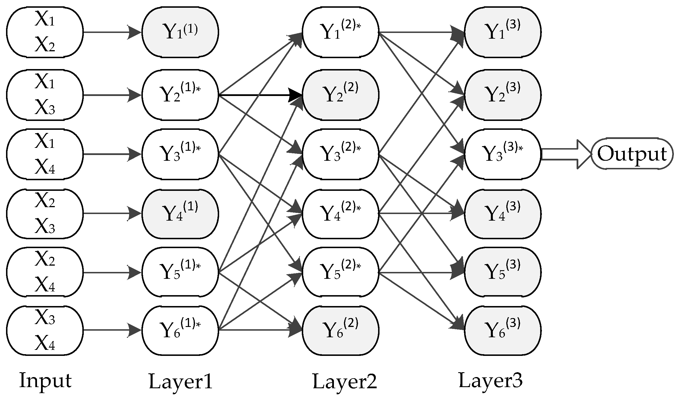
The input data of GMDH is composed of multiple sets of external factor variables and observed values. The variables describing external factors are called characteristic variables, and the characteristic variables and observed values are collectively referred to as input variables. Input data is first divided into a training set and testing set according to a certain proportion by the GMDH algorithm. The training sample data is used for the estimation of the coefficients of the Kolmogorov–Gabor (K–G) polynomial. The testing set is supplied to the GMDH network for error checking. Then, the characteristic variables of the training set are cross-recombined in pairs, and the corresponding observation hold value does not change. After recombination, each pair of characteristic variables is a group and is trained as a neuron of the network. The output of each neuron is a high-order function of both its input, which is referred to as a K–G polynomial function. Then, the output of each neuron is evaluated and tested by an external criterion. We eliminated the neurons that were predicted the worst, and retain the neurons with a good performance as the next layer. The entire process of restructuring, training, testing, and selection was performed again on this new layer. The GMDH network is not completed until the forecast error of the neurons no longer decreases. The GMDH network structure is shown in Figure 1.

In Figure 1, the input column is cross-recombined by all the characteristic variables of the training set. Each reconstructed neuron consists of any two characteristic variables. Suppose there are N groups of data in the input data, each group of data has m characteristic variables and 1 observation value. The number of combinations is given by:

$$k=\frac{m\times (m-1)}{2},$$

(1)

where, m denotes the number of characteristic variables. Cross-recombination of any two characteristic variables can fully express all of the combinations between characteristic variables, and it is easy to determine the effect of each characteristic variable on the observed value. There are only two characteristic variables for each neuron, which enables rapid screening of neurons at lower complexity and acquisition of a suitable model.

In Figure 1, x is the input characteristic variable and y is the observed value, that is, the output variable of each neuron. The output of the previous layer is the input of the next layer. The relationship between the input and the output of each neuron can be represented by a K–G polynomial:

$${\stackrel{\wedge }{y}}_n=f(x_1,x_2,\dots ,x_m)={\displaystyle \sum _{i=1}^m{a}_i{x}_{in}}+{\displaystyle \sum _{i=1}^m{\displaystyle \sum _{j=1}^m{a}_{ij}{x}_{in}{x}_{jn}+}}{\displaystyle \sum _{i=1}^m{\displaystyle \sum _{j=1}^m{\displaystyle \sum _{k=1}^m{a}_{ijk}{x}_{in}{x}_{jn}{x}_{kn}}}}+\cdots ,$$

(2)

where, a_i is the K–G polynomial coefficient and f is the output. When only two characteristic variables are the inputs for each neuron, the second-order K–G polynomial is:

$${\stackrel{\wedge }{y}}_n=f(x_{in},x_{jn})=a_0+a_1{x}_{in}+a_2{x}_{jn}+a_3{x}_{in}{x}_{jn}+a_4{x}_{in}^2+a_5{x}_{jn}^2,$$

(3)

Gray neurons in Figure 1 are the neurons that have been excluded after screening by external criteria. The regularity criteria can be expressed by Equation (4), where $y_n$ is the observed value, ${\widehat{y}}_n$ is the corresponding estimated value of $y_n$, and w is the calculation result of the external criterion. GMDH determines the correlation between neurons and the observed value by the size of the threshold w and selects neurons. The smaller the w calculated by the external criterion, the better the neuron and the better the K–G polynomial fitting effect. The poorer neurons are rejected, and the excellent neurons are preserved and become the input of the next layer. Meanwhile, the minimum $w_{min}$ of this layer is recorded. When the $w_{min}$ of this layer is no longer reduced relative to the previous layer, it indicates that the prediction error of the network is no longer decreasing; then, the network stops expanding, and the result of the previous layer is output. P is the number of test sets.

$$w=\frac{{\displaystyle {\sum }_{n=1}^P{({\stackrel{\wedge }{y}}_n-y_n)}^2}}{{\displaystyle {\sum }_{n=1}^P{(y_n)}^2}},$$

(4)

Traditionally, the coefficient of the K–G polynomial is estimated by the least square method, and the calculation process is as follows:

$$\{\begin{array}{l}{\stackrel{\wedge }{y}}_n=a_0+a_1{x}_{in}+a_2{x}_{jn}+a_3{x}_{in}{x}_{jn}+a_4{x}_{in}^2+a_5{x}_{jn}^2\\ e={\displaystyle {\sum }_{n=1}^N{(y_n-{\stackrel{\wedge }{y}}_n)}^2}\\ \frac{\partial e}{\partial a_k}=0k=0,1,2,3,4,5\end{array},$$

(5)

In order to facilitate the analysis, the results are expressed in matrix form:

$$\mathit{a}={({\mathit{X}}^{\mathit{T}}\mathit{X})}^{-1}{\mathit{X}}^{\mathit{T}}\mathit{y},$$

(6)

where,

$$\mathit{X}=\left\{\begin{array}{cccccc}1& x_{i1}& x_{j1}& x_{i1}{x}_{j1}& x_{i1}^2& x_{j1}^2\\ 1& x_{i2}& x_{j2}& x_{i2}{x}_{j2}& x_{i2}^2& x_{j2}^2\\ 1& x_{i3}& x_{j3}& x_{i1}{x}_{j2}& x_{i3}^2& x_{j3}^2\\ ⋮& ⋮& ⋮& ⋮& ⋮& ⋮\\ 1& x_{in}& x_{jn}& x_{in}{x}_{jn}& x_{in}^2& x_{jn}^2\end{array}\right\},$$

(7)

and a is polynomial coefficient, $\mathit{a}=(a_0,a_1,a_2,a_3,a_4,a_5)$. y is the observed value, $\mathit{y}=\left(y_1,y_2,\dots ,y_N\right)$.

This calculation process requires the least square method to meet the basic assumption of the linear regression model. One of the important assumptions is that there is no linear relationship between variables in the regression model [28]. In short-term load forecasting, when the input variable has multicollinearity, ${\mathit{X}}^T\mathit{X}$ does not have an inverse matrix, so Equation (6) cannot be solved. This results in severe distortion of the parameter estimation and a decrease in GMDH prediction accuracy. Therefore, this paper uses elastic net instead of the least square method to estimate the K–G polynomial coefficient and thereby solve the problem of multiple multicollinearity and overfitting in the estimation of the least square method. Moreover, the elastic net uses the L1 norms and L2 norms as prior regular terms to obtain a more stable and practical regression equation through the compression regression coefficient.

3. Elastic Net

Elastic net is a revised variable selection algorithm based on lasso. To overcome the deficiencies of traditional biased estimation methods, such as stepwise regression and ridge regression, in the selection of variables, such as poor anti-interference ability, Tibshirani proposed the lasso algorithm, which has had breakthrough significance [34,41,42]. There is the observed value $\mathit{Y}\in R^{N\times 1}$ and an input matrix $\mathit{X}\in R^{N\times m}$, and we approximate the regression function by a linear model $\mathrm{E}\left(\mathrm{Y}|\mathrm{X}=x\right)=a_0+x^{T}a$. The regression model of lasso is:

$$\{\begin{array}{l}\stackrel{\wedge }{\mathit{a}}=\underset{(a_0,a)\in R^m}{\min }\left[\frac{1}{2N}{\displaystyle \sum _{n=1}^N{\left(y_n-{\mathit{a}}_0-x_n^T\mathit{a}\right)}^2}+\lambda {\Vert \mathit{a}\Vert }_1\right]\\ {\Vert \mathit{a}\Vert }_1={\displaystyle \sum _{j=1}^m\left|a_j\right|}\end{array},$$

(8)

the first term on the right is the least square term, and the second is the penalty term, where a is the regression coefficient; $\Vert \mathit{a}{\Vert }_1$ is the L1 norm, which is the sum of the absolute values of all elements in the matrix and λ is a penalty parameter and has the effect of a compression variable, and its numerical value indicates the severity of punishment.

By punishing the sum of the absolute value of the regression coefficient, lasso realizes the compression regression coefficient, making the partial regression coefficient strictly equal to zero. That makes the lasso sparse and avoids overfitting problems. Sparseness will make the lasso have two characteristics, one is feature selection. There are some elements in the input data that are not related to the observed values. When solving the minimum residual error, although this part of the elements will reduce the training error, this part of the unrelated elements will interfere with the prediction model when predicting new samples, resulting in overfitting. Feature selection can accurately screen out irrelevant information. The second characteristic is interpretability. Among the many input data, there are always some elements that have a decision-making influence on the observation value. The identification of this part can accurately describe the characteristics of the model and make the model principle highly transparent and clear, so that the model has a strong interpretation. However, the lasso cannot handle multicollinearity, and Zou et al. and Hanstie et al. proposed an elastic net based on the lasso to address these deficiencies.

Elastic net is the first sparse model with an automatic group effect [34], and the model is:

$$\{\begin{array}{l}\stackrel{\wedge }{\mathit{a}}=\underset{(a_0,a)\in R^m}{\min }\left[\frac{1}{2N}{\displaystyle \sum _{n=1}^N{\left(y_n-{\mathit{a}}_0-x_n^T\mathit{a}\right)}^2}+{\lambda }_1{\Vert \mathit{a}\Vert }_1+{\lambda }_2{\Vert \mathit{a}\Vert }_2^2\right]\\ {\Vert \mathit{a}\Vert }_1={\displaystyle \sum _{j=1}^m\left|a_j\right|}\\ {\Vert \mathit{a}\Vert }_2^2={\displaystyle \sum _{j=1}^m{a}_j^2}\end{array},$$

(9)

where the first term on the right of the equal sign is the loss function and the second and third terms are penalty terms. $\Vert \mathit{a}{\Vert }_2^2$ is the L1 norm, which represents the sum of the squares of all elements of the matrix, which is the Euclidean distance. λ is a penalty parameter. Specifically, ${\lambda }_1$ is a one-norm penalty and ${\lambda }_2$ is a second-norm penalty. Both the L1 norm and L2 norm have the function of the compressive regression coefficient. Elastic net compresses the regression coefficient twice and leads to an increase in estimation bias. Therefore, it is necessary to improve the above formula.

Letting $\alpha =\frac{{\lambda }_1}{{\lambda }_1+{\lambda }_2}$, $\lambda ={\lambda }_1+{\lambda }_2$:

$$\stackrel{\wedge }{\mathit{a}}=\underset{(a_0,a)\in R^m}{\min }\{\frac{1}{2N}{\displaystyle \sum _{n=1}^N{\left(y_n-{\mathit{a}}_0-x_n^T\mathit{a}\right)}^2}+\lambda \left[\alpha {\Vert \mathit{a}\Vert }_1+\frac{\left(1-\alpha \right)}{2}{\Vert \mathit{a}\Vert }_2^2\right]\},$$

(10)

where α is the weight factor of the L1 norm and L2 norm.

It can be seen that when ${\lambda }_2=0$, the penalized term is the L1 norm and the elastic net becomes a lasso regression. Its sparseness can automatically select characteristic variables, reduce model complexity, improve model generalization ability, and avoid overfitting.

When ${\lambda }_1=0$, the penalty term is the L2 norm and elastic net becomes a ridge regression. The L2 penalty term added by the ridge regression makes $\left|{\mathit{X}}^T\mathit{X}+\lambda \mathbf{I}\right|$ a nonsingular matrix, guaranteeing that $\mathit{a}={\left({\mathit{X}}^T\mathit{X}+\lambda \mathbf{I}\right)}^{-1}{\mathit{X}}^T\mathit{y}$ can be obtained. The prediction error consists of two parts, the deviation and the variance. The least square is an unbiased estimate whose mathematical expectation is equal to the true value of the estimated parameter. The existence of multicollinearity in the input variable will increase the variance of the least squares, and the parameter estimation will be seriously distorted. Ridge regression solves this problem by adding a minimum deviation value $\lambda \mathbf{I}$ to the regression estimate. The deviation of the increase of the ridge regression makes the least squares give up the unbiasedness, and the error increases, but compared with the large variance caused by multicollinearity, the regression coefficient is obtained by the ridge regression at the cost of losing part of the information and reducing the accuracy is more realistic, avoiding the adverse effects caused by multicollinearity.

4. Variable Weight Input Based on Difference Degree

The concept of the difference degree refers to the difference in size due to the characteristics (such as temperature and wind speed) of the two samples. The smaller the difference degree, the closer the characteristics of various factors between the two samples are. Short-term load forecasting generally needs to refer to historical data such as the load and its characteristic factors in the days before the forecast. The smaller the date difference between historical data and forecast day, the closer the fitting law of the characteristic factors and load is to the fitting law of the forecast day. Therefore, this paper treats historical data differently based on the difference between the date and the difference degree between the days [1].

The idea of weighting input data based on the difference is as follows. First of all, calculate the difference degree between any two days; then, the weights of each day are calculated according to the difference degree and the difference degree is reflected by the size of the weight. Based on the time sequence, the historical data close to the forecast time have significant weight, while the historical data far away from the forecast time have small weight; finally, when fitting the polynomial coefficients, the weights calculated based on the difference degree are assigned to the historical data of the corresponding days for the next calculation.

The Lance–Williams distance is used to calculate the difference degree. The Lance–Williams distance is one of the commonly used clustering algorithms, proposed by Lance and Williams. The distance in cluster analysis is used to measure the similarity and difference between samples, which is the key step of cluster analysis. Compared with the typical method Euclidean distance, the Lance–Williams distance is insensitive to singular values, which can suppress the influence of noise and handle highly skewed data. In addition, it is a dimensionless standardized value that can eliminate the influence of data due to dimensional differences, so the calculated value of the Lance–Williams distance is used to describe the difference degree [1,43]. The value of the Lance–Williams distance is the value of the difference. The smaller the value, the smaller the difference between the two sample data, the greater the contribution of the sample data in the model training.

Set m characteristic variables and t group sample data. The Lance–Williams distance is:

$$d_{ij}={\displaystyle \sum _{t=1}^m\frac{\left|x_{it}-y_{jt}\right|}{\left|x_{it}+y_{jt}\right|}},$$

(11)

where $x_{ik},y_{jk}\ge 0$,$i,j=1,2,3,\dots ,t$. And $i\ne j,i<j$. $d_{ij}$ represents the Lance–Williams distance between the ith sample and the jth sample.

Calculate the weight of each sample by the different $d_{ij}$ according to the above formula. Let the weight of each sample be $w_i^{\ast }\left(i=1,2,3,\dots ,t\right)$. Then:

$$\{\begin{array}{l}\frac{w_1-w_2}{w_1+w_2}=d_{12}\\ \frac{w_1-w_3}{w_1+w_3}=d_{13}\\ \hfill ⋮\hfill \\ \frac{w_1-w_t}{w_1+w_t}=d_{1t}\\ \frac{w_2-w_1}{w_2+w_1}=d_{21}\\ \frac{w_2-w_2}{w_2+w_2}=d_{22}\\ \hfill ⋮\hfill \\ \frac{w_{t-1}-w_t}{w_{t-1}+w_t}=d_{t-1t}\end{array},$$

(12)

get W = $\left(w_1,w_2,w_3,\dots ,w_t\right)$. Thus, the weight $w_i^{\ast }$ can be obtained:

$$w_i^{\ast }=\frac{w_i}{{\displaystyle \sum _{i=1}^t{w}_i}},$$

(13)

The weight $w_i^{\ast }$ satisfies the following conditions:

• ${\displaystyle \sum _{i=1}^t{w}_i^{\ast }=1}$
• $w_1^{\ast }\ge w_2^{\ast }\ge w_3^{\ast }\ge \dots w_t^{\ast }$
• $0<w_i^{\ast }\le 1$

5. Establish the Short-Term Load Forecasting Model

5.1. The Selection of the Parameter α and λ

In Equation (10), the selection of the parameters α and λ have an important influence on the performance of the model. Before calculating the parameters, the input variables are centralized and standardized first. This allows different variables describing different characteristics to be calculated on the same scale.

The parameter α is equally-spaced and traverses the values in the range of $(0,1]$. The smaller the value spacing, the higher the calculation accuracy and the longer the calculation takes time. According to the calculation experience, the value spacing is selected as 0.02, and then determines the value of α according to the Mean Square Error (MSE) of the prediction result.

For λ, ${\lambda }_{\max }$ needs to be calculated first. Given characteristic variables matrix $\mathit{X}=\left[{\mathit{x}}_1,{\mathit{x}}_2,\dots ,{\mathit{x}}_m\right]$, where ${\mathit{x}}_m={\left[x_{1m},x_{2m},\dots ,x_{Nm}\right]}^T$. Observed matrix $\mathit{Y}={\left[y_1,y_2,\dots ,y_N\right]}^{\mathit{T}}$. First, the average value of each column of the matrix is obtained [41]:

$$\begin{array}{l}{\mathit{X}}_{ave}=\left[x_{ave1},x_{ave2},\dots ,x_{avem}\right]\\ Y_{ave}\end{array}$$

(14)

Subtract the average value of the corresponding column from each element of matrix X and matrix Y:

$$\begin{array}{l}{\mathit{X}}_d=\left[{\mathit{x}}_{d1},{\mathit{x}}_{d2},\dots ,{\mathit{x}}_{dm}\right]=\left[{\mathit{x}}_1-x_{ave1},{\mathit{x}}_2-x_{ave2},\dots ,{\mathit{x}}_m-x_{avem}\right]\\ {\mathit{Y}}_d=\mathit{Y}-Y_{ave}\end{array}$$

(15)

then obtain:

$$\begin{array}{l}{\lambda }_{\max }=\frac{\max \left|{\mathit{X}}_d^T\times {\mathit{Y}}_d\right|}{N\alpha }\\ {\lambda }_{\min }=\epsilon {\lambda }_{\max }\end{array}$$

(16)

The typical value of ε is 0.001. In the range of $\left[{\lambda }_{\min },{\lambda }_{m\mathrm{ax}}\right]$, the equally-spaced 100 values are taken into Equation (10), and then the optimal λ is selected through five-fold cross-validation.

5.2. The Main Factors Influencing Load Forecasting

The proportion of the meteorological sensitive load in the total load is increasing, and meteorological factors have become the primary factors affecting short-term load forecasting. The main meteorological factors that affect the load are temperature, humidity, rainfall, wind speed, and others [44,45]. Temperature is the primary meteorological factor that affects the load [46].

The cumulative effect of meteorological factors cannot be ignored either. Because human senses have an adaptation process to meteorological changes, the predicted days will be affected by the accumulation of temperature or humidity in previous days. It shows that the change in daily load is delayed by meteorological changes, and we call it the accumulation effect of meteorological factors. The cumulative effect is mainly affected by the meteorological factors three days before the predicted date, in which the cumulative effect of temperature and relative humidity is most prominent [47,48]. Combined with the other load factors selected in this paper, the influence of temperature and relative humidity on short-term load forecasting is considered in this paper. Due to the different degrees of cumulative effect caused by temperature and relative humidity, temperature and relative humidity were addressed by referring to the THI used by the USA PJM market [1].

$$THI=Tem{p}_F-(0.55-0.55Hmd)\times (Tem{p}_F-58),$$

(17)

where $Tem{p}_F$ represents temperature, with the units as degrees Fahrenheit, and Hmd is relative humidity. Due to the difference between the meteorological factors of the previous day and the meteorological factors of the two days before the forecast, the THI of the first two days were weighted. The $TH{I}_1$ of the previous day and the $TH{I}_2$ of the previous two days of the forecast are, respectively,

$$TH{I}_1=\frac{4}{5}\times THI,$$

(18)

$$TH{I}_2=\frac{1}{5}\times THI,$$

(19)

where the THI is calculated by Equation (17).

Industrial load accounts for the main part of regional load, and the decrease of industrial load caused by the factory’s holiday is the main factor of the change of holiday load [49,50,51]. Therefore, this paper considers the impact of holidays on load forecasting.

5.3. EN-GMDH Short-Term Load Forecasting

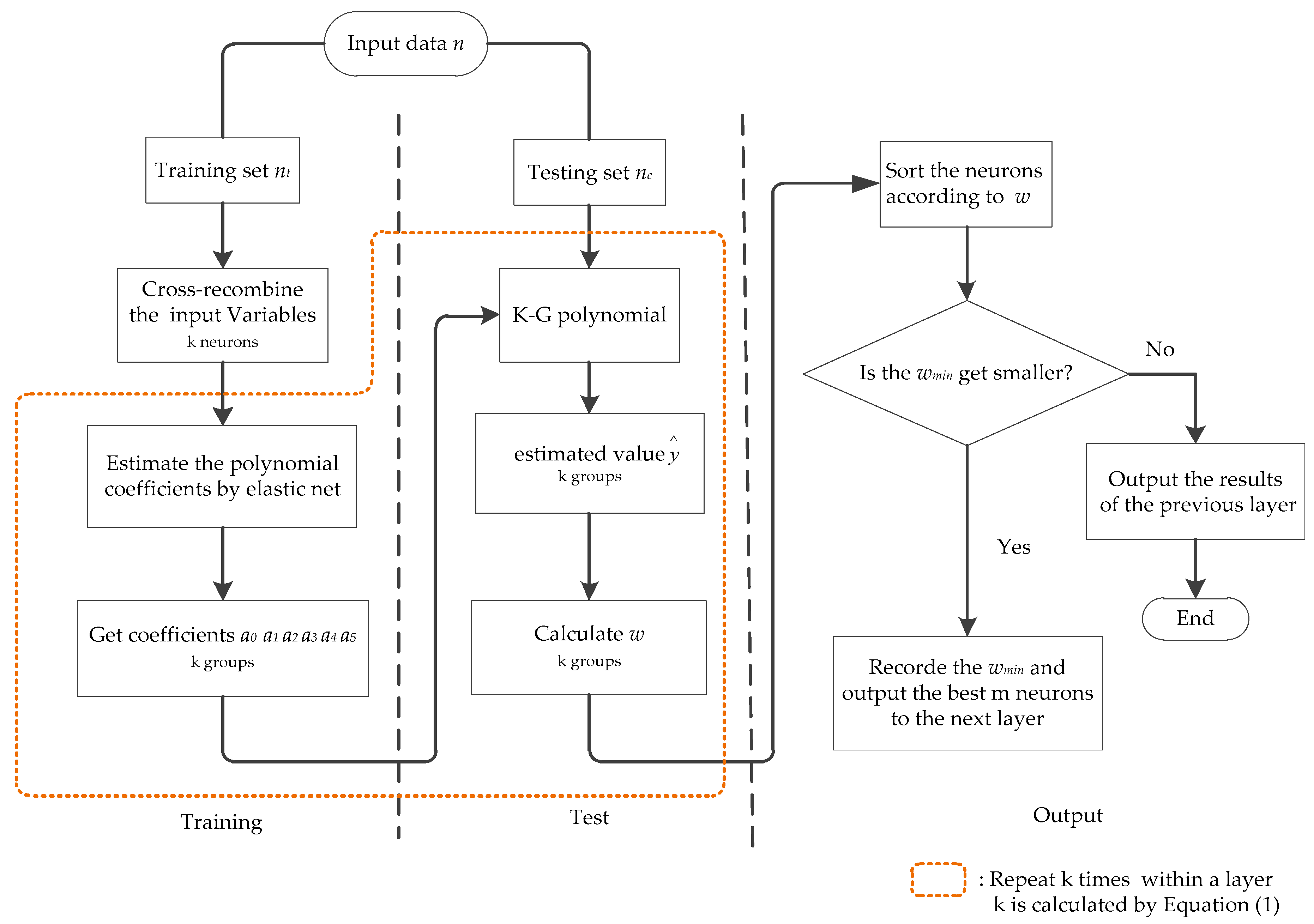
EN-GMDH uses the elastic net to replace least square estimates to estimate the coefficient of the K–G polynomial. The EN-GMDH algorithm flow is shown in Figure 2.

In traditional GMDH, the coefficients of the K–G polynomial are estimated by least square fitting, which has no function of compressing characteristic variables. The characteristic variables with small contributions to load prediction are directly eliminated after the evaluation of external criteria. Although these characteristic variables have little influence on load prediction, their removal will enlarge the prediction error. Elastic net, while estimating the K–G polynomial coefficient, compresses variables with little influence on the output, limiting their contribution to load forecasting rather than eliminating it directly. In this way, the polynomial coefficients can be estimated more accurately.

5.4. Main Mode Steps of EN-GMDH

The detailed modeling steps of the short-term load forecasting model are as follows. The input data consist of multiple sets of input variables. Each set of data contains the characteristic variables influencing the load, such as temperature, holidays, etc., and the load value as the observation value. Set n rows (groups) and m + 1 columns (m columns are characteristic variables, and 1 column is the load value):

Step 1: The input variables are centralized and standardized first. Then 75% of the input variables n are divided into a training set n_t, and the remaining 25% are used as a testing set n_c; n = n_t + n_c.

Step 2: Calculate the difference degree of the training set n_t. Calculate the Lance–Williams distance of the daily data and calculate the weight of the daily data.

Step 3: The 10 characteristic variables of the training set are cross-recombined. By Equation (1), the cross-recombination will produce k (calculated by Equation (1)) neurons. Each neuron contains any two characteristic variables.

Step 4: Take a neuron and corresponding load value into Equation (3). The coefficients a₀, a₁, a₂, a₃, a₄, and a₅ of the K–G polynomial in this neuron are estimated by elastic net, and the obtained coefficients are assigned to this K–G polynomial.

Step 5: Take the testing set data into the K–G polynomial obtained in Step 4 and get estimates of ${\widehat{y}}_j$. Calculate the threshold w of this neuron by taking the ${\widehat{y}}_j$ into Equation (4).

Step 6: Repeat steps 4 to 5, completing the training and inspection of the remaining neurons.

Step 7: Sort the neurons in ascending order according to the threshold w. The first m neurons are retained and output. The remaining k-m neurons are removed, and the minimum w of the layer is recorded.

Step 8: Take the output of the first layer as the input of the second layer, cross-recombine again, and repeat Steps 4 to 7, extending the next layer of the network.

Step 9: The forecast model error will be the minimum value when the lowest regularity criterion ω in the current layer is no longer smaller than that of the previous layer. The network stops expanding, and the model outputs the predicted results

6. Example Analysis

6.1. Example and Data Description

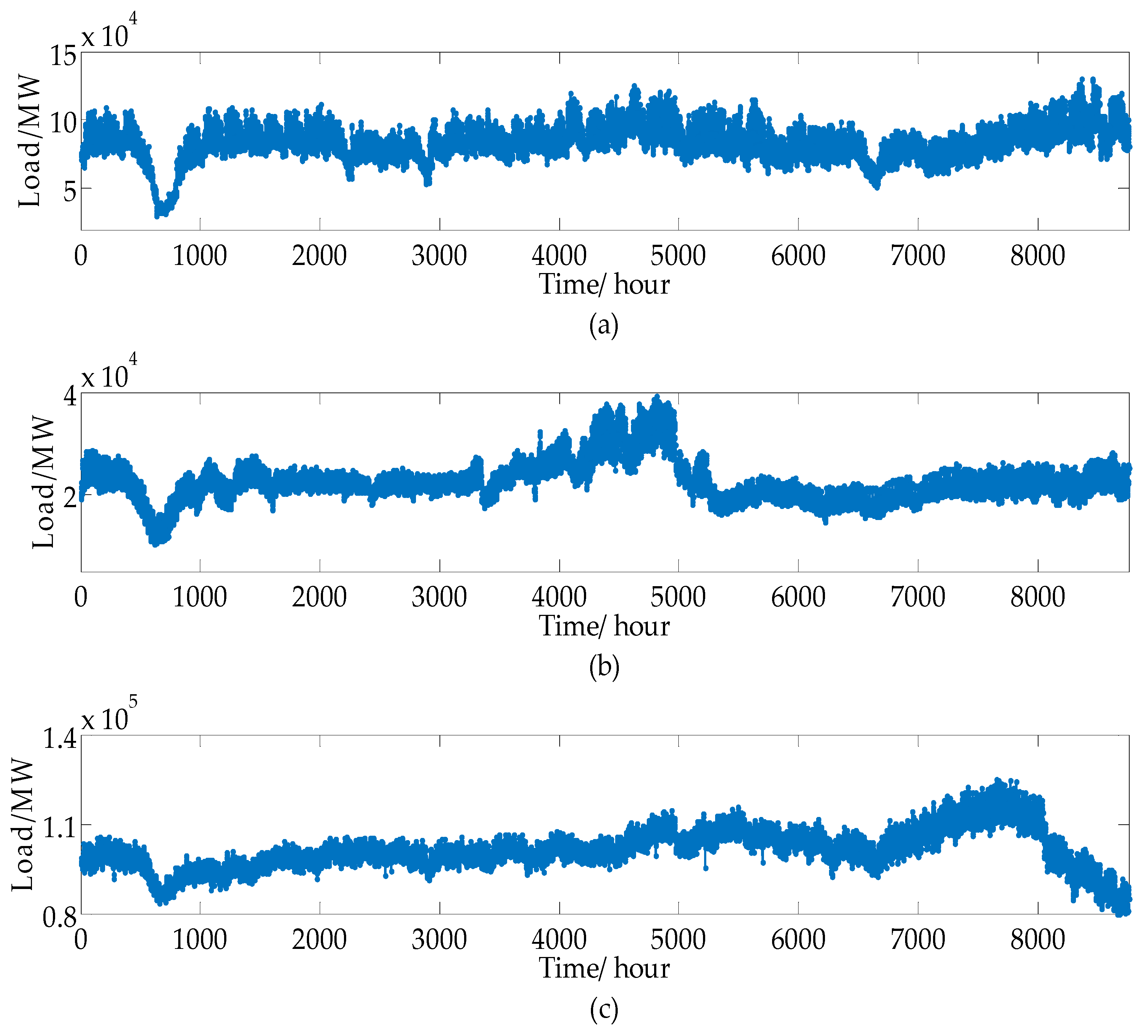
In this paper, data of three northern Chinese cities of Shandong Province for one year were selected for simulation analysis. Although the model EN-GMDH proposed in this paper is used to predict the hourly load of the next day, data of different seasons are selected to verify the generalization performance of this model. Due to the similar climate of the spring and autumn and the short seasonal feature time in these cities, we selected three months of data from each year to represent spring (autumn), summer, and winter. A total of nine data sets were generated in three locations, which are represented by L1 to L9. With one hour of data as a group, there are nine data sets, 270 days, and 6480 h series. Each set of data consists of 11 input variables, including 10 characteristic variables composed of meteorological factors, meteorological accumulation factors, and holiday factors, and 1 load value as the observation value. The annual hourly load of the three cities is shown in Figure 3.

According to the grouping rule of the GMDH algorithm, 75% of the input data is used as the training set and 25% as the testing set. This paper uses MATLAB (R2017b, MathWorks, Natick, MA, USA, 2017) to build the prediction model and used MATLAB’s lasso.m function. The software operating environment uses a quad-core processor and 8 GB of memory. To improve the speed of operation, this paper uses the MATLAB parallel toolbox to run the program.

The hourly data set used in this paper is composed of 11 input variables: extreme wind speed, maximum wind speed, hourly rainfall, average temperature, maximum temperature, relative humidity, minimum humidity, THI of the previous day, THI of the previous two days, holidays, and load value. All of the data types are shown in

Table 1. Categories of input variables

Input Variables	Categories	Introduction
1	meteorological factors	extreme wind speed
2		maximum wind speed
3		hourly rainfall
4		average temperature
5		maximum temperature
6		relative humidity
7		minimum humidity
8	meteorological accumulation factors	$TH{I}_1$
9		$TH{I}_2$
10	holiday factors	Differentiating holidays, weekends, and working days by numerical values.
11	load	Each set of characteristic variables corresponds to a load value. The load value of the training set is used for training the model, and the load value of the testing set is used for testing the error.

.

6.2. Model Analysis

In order to show the operation process of the model and the changes of related parameters, a small amount of data (only four days of data) is selected to input the model. The variation trend of model parameters and output can be observed by calculating the actual data.

6.2.1. Multicollinearity Test

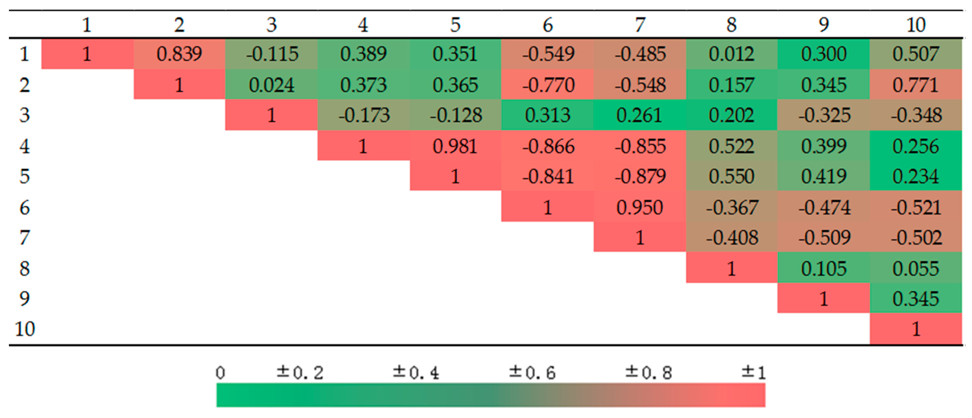
First, the Spearman rank correlation coefficient analysis was performed on the characteristic variables of sample data 1 to test whether there is multicollinearity [52]. Spearman rank correlation analysis is a linear correlation analysis using the rank order size of two variables. It is a type of statistical quantity obtained by replacing the actual data with the rank of each factor sample value. The calculation formula is presented in Equation (20). By calculating the characteristic variables, the correlation coefficient ρ between each of the two characteristic variables was obtained, as shown in Figure 4.

$$\rho =1-\frac{6{\displaystyle \sum d^2}}{n^3-n},$$

(20)

where d is the difference between the ranks of the two columns and n is the length of each column.

In general, there is a linear correlation between variables when $\rho >0.8$. Linear correlation is a sufficient condition for multicollinearity. From Figure 4, it can be seen that the selected characteristic variables have obvious multicollinearity, which will make the coefficient estimation unstable.

Removing secondary or alternative explanatory variables is a common method for solving multicollinearity. However, it is a rigorous process to determine the alternative explanatory variables; improper deletion can cause serious deviation in parameter estimation. Furthermore, the alternative explanatory variables that are deleted still contain useful information for load forecasting and deleting them will increase the error of the prediction.

6.2.2. Operation of the Model

To test the performance of the EN-GMDH short-term load prediction model, a small amount of data is input into the model and analyzed in detail.

According to the network expansion rule of EN-GMDH, when a layer of w_min is no longer reduced, the network will not be expanded. By calculation, the w_min of the second layer of the model network is greater than that of the first layer of the network, indicating that the prediction error is no longer reduced and that the network stops expanding. A two-layer GMDH network model was obtained. The model-related parameters are shown below.

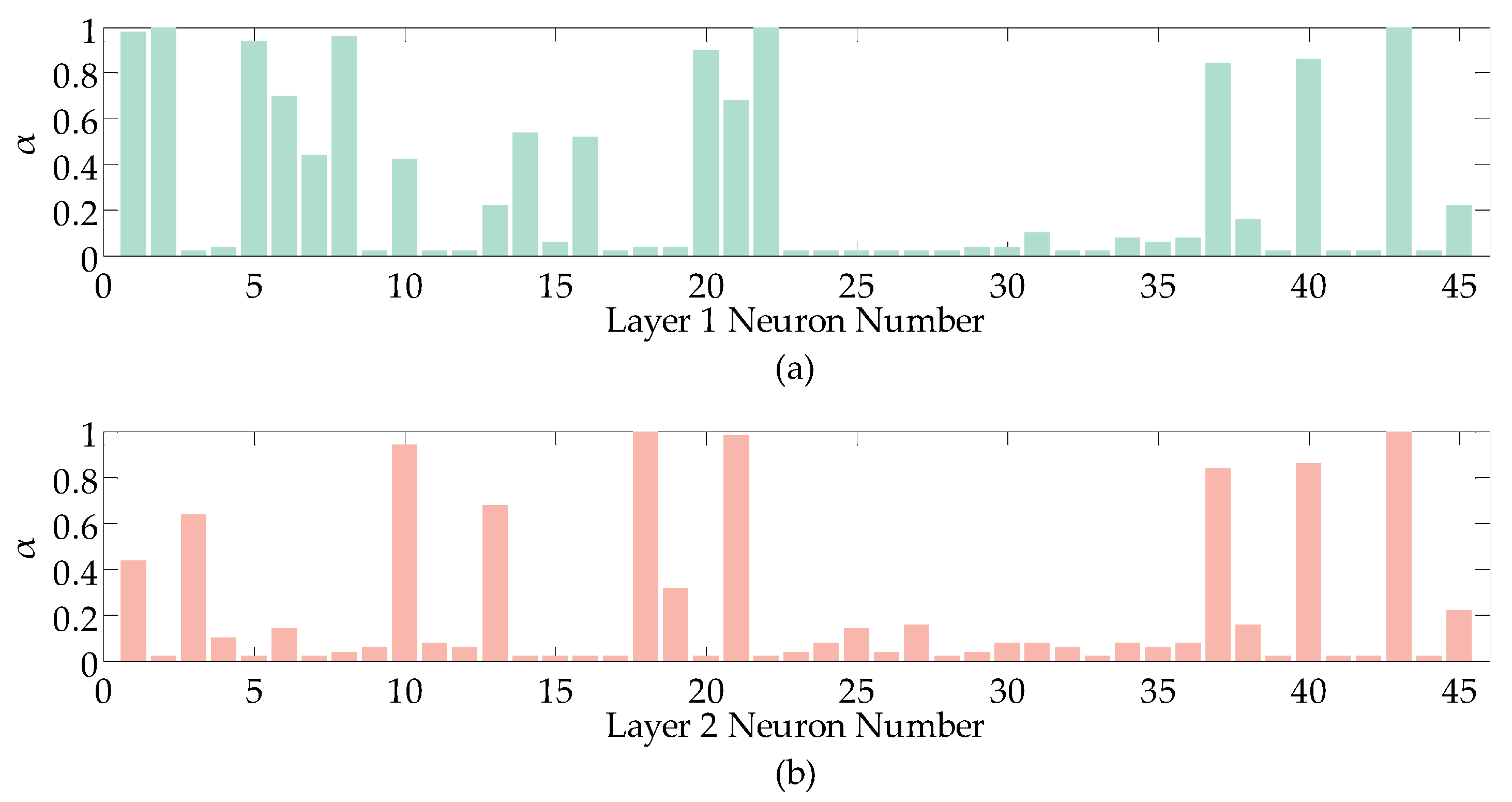
The parameter α in elastic net traverses the values in the range of $(0,1]$. Each neuron in each layer of the network requires an optimal α for the weight balance of lasso and ridge regression in Equation (10). The α can be assigned in two ways. One is to assign α directly to the empirical value. This method has a small amount of computation, however it is easy to expand the error and requires existing experience as a reference. Another method is to take a value for α traversal and select according to the minimum MSE of the predicted results. This method has a large amount of computation but small error, which is employed in this paper. In the model, the first layer and the second layer of the network each produce 45 optimal α. The selected α value of the first layer of network neurons is shown in Figure 5a, and the selected α value of the second layer of network neurons is shown in Figure 5b.

α = 1 denotes that Equation (10) is lasso regression, and α→0 denotes that Equation (10) is a ridge regression. The value of α is between 0 and 1 denotes that Equation (10) is elastic net. Through each α in this picture, you can see the characteristics of the data. α is close to 1, which indicates that there is a heavy overfitting of data. At this time, elastic net produces sparseness through the L1 norm penalty to avoid large error. α is close to 0, indicating that there is a heavy multicollinearity phenomenon in the data. At this time, elastic net can guarantee the stability and accuracy of the model through the L2 norm penalty compression regression coefficient. It can be seen from Figure 5 that the point where α is less than 0.5 accounts for the majority, indicating that the data has significant multicollinearity. The process of α change is the presentation of multicollinearity and overfitting problem solved by EN-GMDH.

After estimating the coefficients of the K–G polynomial by elastic net, the polynomial coefficients of the model output are as shown in

Table 2. Kolmogorov-Gabor (K–G) polynomial coefficients.

Coefficient Name	Value	Coefficient Name	Value
$a_0$	49.19759	$a_3$	0.00003
$a_1$	0.48066	$a_4$	−0.01520
$a_2$	1.84231	$a_5$	−0.00775

.

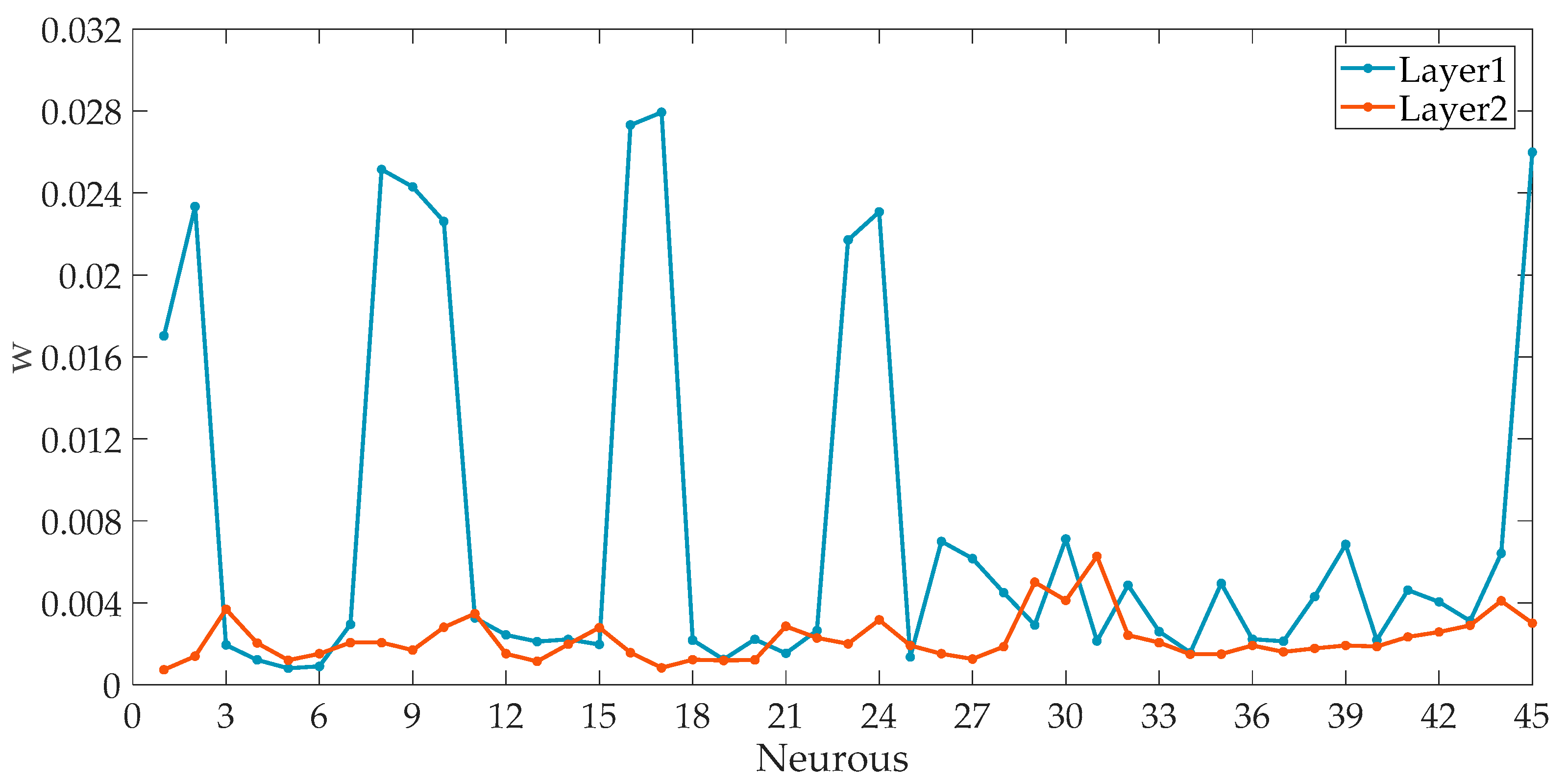
The 45 neurons in each layer of the network need to be taken into the external criterion of Equation (4) to calculate their w to judge the performance of each neuron. The w values of neurons in the first layer and second layer of the network are shown in Figure 6.

As shown in Figure 6, the blue line represents the w calculated by Equation (4) of the neurons in the first layer of the network. The brown line represents the w of the second-layer neurons of the network. The input of the first layer of the network contains all the characteristic variables. As seen in Figure 6, the w value of each neuron differs greatly. This indicates that different characteristic variables have different contributions to load forecasting. In the second layer of the network, only the excellent neurons in the first layer are selected as input data. Compared with the neurons of the first layer, the performance of the neurons of the second layer is more stable and excellent.

According to the w size of each layer, the first ten neurons of the first layer and the first ten neurons of the second layer were selected, and the w are shown in

Table 3. w for neurons selected of each layer.

Network Layer 1				Network Layer 2
Neuron Number	w	Neuron Number	w	Neuron Number	w	Neuron Number	w
5	0.00081	21	0.00154	1	0.00074	18	0.00123
6	0.00090	34	0.00157	13	0.00115	35	0.00150
4	0.00122	3	0.00195	19	0.00119	12	0.00152
19	0.00124	12	0.00204	5	0.00120	26	0.00152
25	0.00136	13	0.00211	20	0.00122	16	0.00157

.

The $R^2$ of the first and second layer is shown in

Table 4. The $R^2$ of each layer.

Layer	${\mathit{R}}^2$
1	0.792
2	0.673

. The $R^2$ is the measurement value of the fitting degree. Here, it represents the interpretation degree of the characteristic variables compared to the observed value. The closer the value is to 1, the better the fitting degree of the regression equation is, and the better the prediction effect is. It can be seen from Table 4 that this model has a good data fitting effect when training.

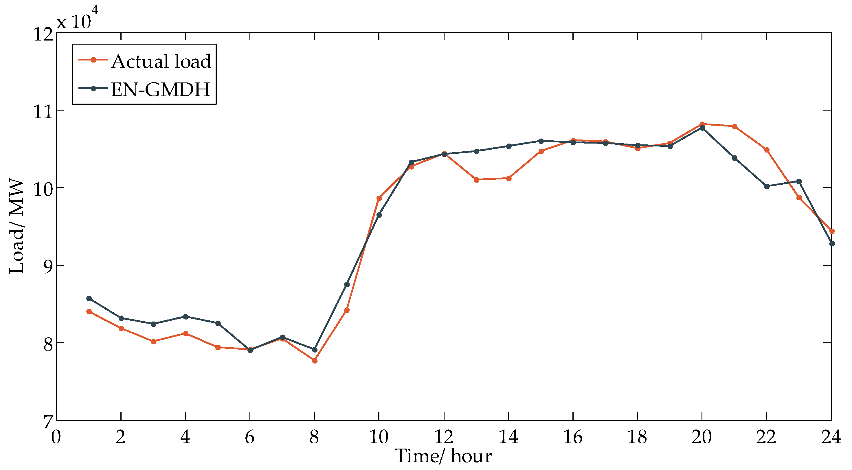
Through the above model, which forecasts the hourly load of the next day, the load forecast curve is as shown in Figure 7.

6.3. Evaluation Metrics

The forecasts are evaluated using the MAE, sMAPE, and MASE. The MAE is a commonly used metric, representing the mean value of the sum of absolute differences between actual and forecasted. Meanwhile, sMAPE is another effective metric used, which is an alternative to Mean Absolute Percent Error (MAPE) when there are zero or near-zero demand for items; sMAPE self-limits to an error rate of 200%, reducing the influence of these low volume items [9,53].

$$\mathrm{MAE}=\mathrm{mean}(|y_n-{\stackrel{\wedge }{y}}_n|),$$

(21)

$$\mathrm{sMAPE}=\mathrm{mean}\left(200\frac{|y_n-{\stackrel{\wedge }{y}}_n|}{|y_n|+|{\stackrel{\wedge }{y}}_n|}\right),$$

(22)

Furthermore, this paper also uses the MASE proposed by Hyndman and Koehler [54]. The molecular part of Equation (23) is defined as the mean absolute error for the test set, and the denominator part is defined as the mean absolute error of a benchmark method on the training set. The MASE needs a scaling factor that can provide the help of the error measured by a benchmark method, where normally the naïve method is used. When we calculate the MAPE, we first need to select the naïve method as a benchmark method, which uses the last known reference value as forecast.

$$\mathrm{MASE}=\frac{\mathrm{mean}(|y_n-{\stackrel{\wedge }{y}}_n|)}{\mathrm{mean}(|y_i-{\stackrel{\wedge }{y}}_{i-m}|)},$$

(23)

where the denominator part of Equation (23) is the analytical form of naïve method based on the training set. The m represents the forecast period. When the MASE < 1, the proposed method performs better than the naïve method. When the MASE > 1, the proposed method is inferior to the naïve method [9,53].

6.4. Time Series Cross-Validation

Cross-validation is one of the most important tools in the evaluation of regression methods. It is often used to avoid overfitting and evaluation in time series forecasting. However, the standard cross-validation is restricted in traditional time series forecasting due to both theoretical and practical problems. To get a valid estimation of models performance, time series cross-validation is used in this paper.

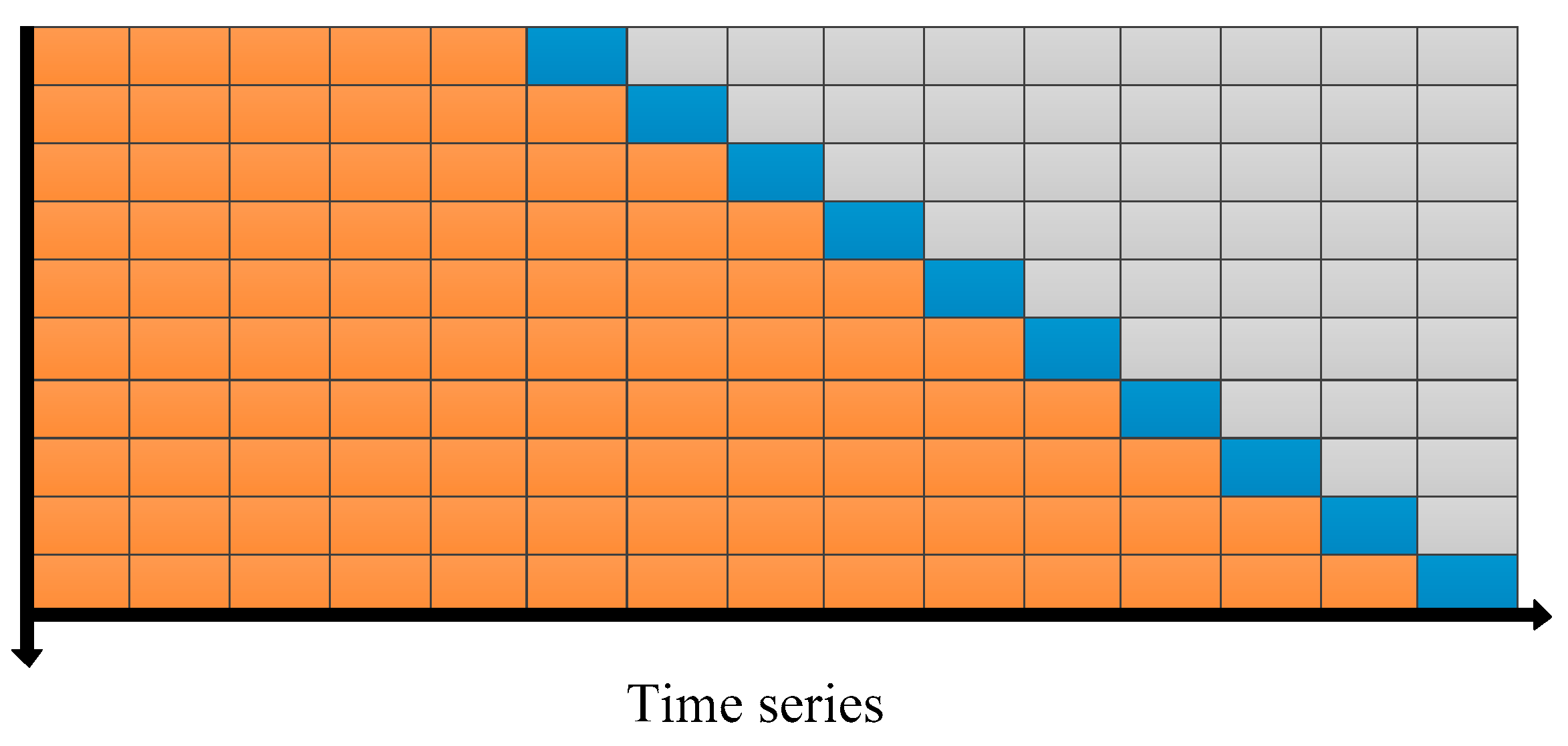
The principle of time series cross-validation is also described as “evaluation on a rolling forecasting origin”. Its principle can be shown in Figure 8. There is a series of data, the test set are performed by sequentially moving in order of time. The corresponding training set consists only of the data previously used for testing. The training set origin is fixed but the end point keeps changing. For each forecast, the model is recalibrated using all available data in the training set after update. The forecast error evaluation is computed by averaging overall the test sets that typically will be more robust than single measures [53].

6.5. Analysis of Prediction Results

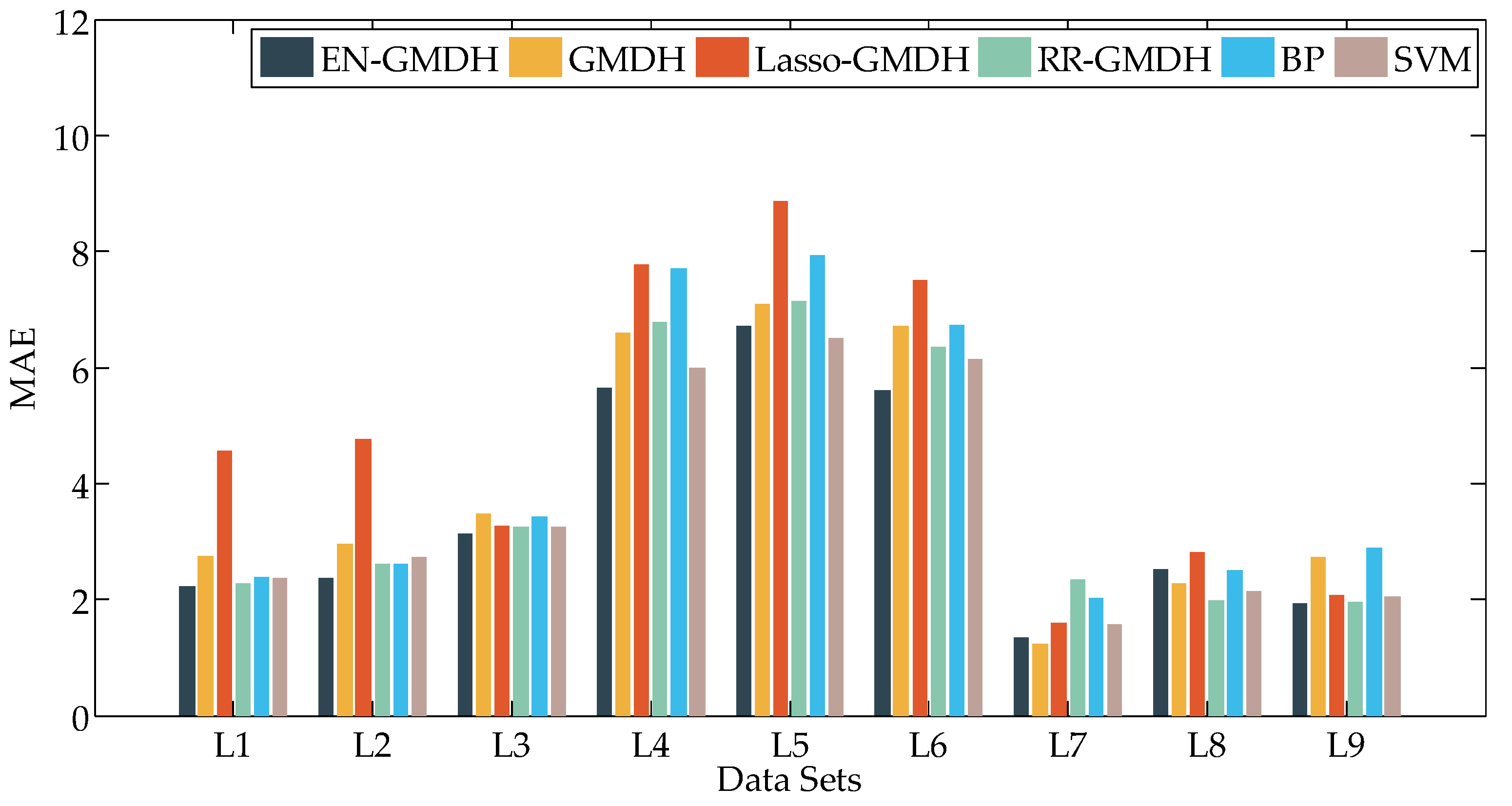
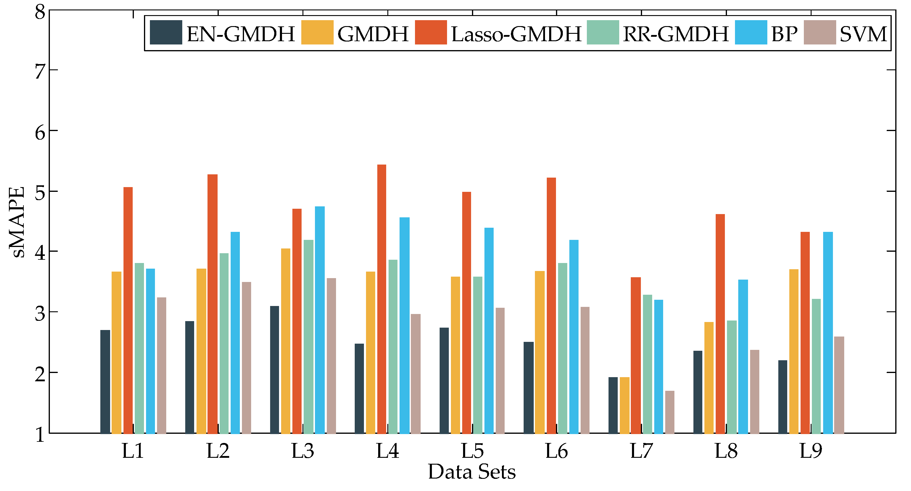
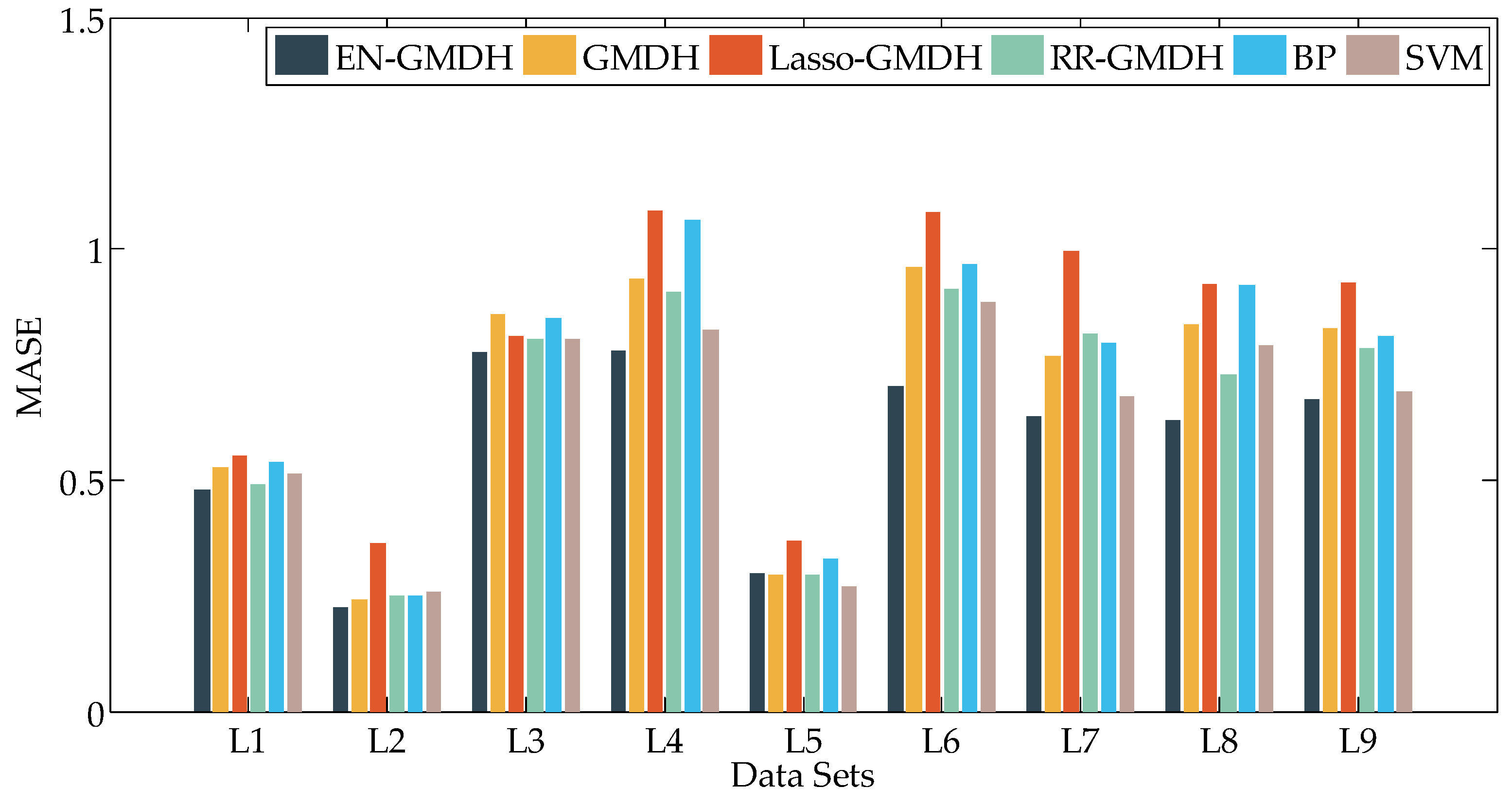
In this paper, the EN-GMDH algorithm is compared with the other five algorithms to test the performance of the EN-GMDH model in short-term load forecasting. The other five algorithms are GMDH, Lasso-GMDH using lasso regression to replace the GMDH least squares part, group method of data handling based on ridge regression (RR-GMDH) using ridge regression to replace the GMDH least squares part, the back propagation (BP) neural network, and support vector machine (SVM), which is widely used in the load forecasting neural field. The sample datasets L1 to L9 are sequentially brought into all of the above models for load forecasting, and the forecast results are compared.

Figure 9, Figure 10 and Figure 11 are the graphs and bars of load forecasting by six algorithms accordingly from L1 to L9. Figure 9 represents MAE, Figure 10 represents sMAPE, and Figure 11 represents MASE.

Table 5. Evaluation Results. EN-GMDH: group method of data handling based on elastic net; RR: ridge regression; BP: back propagation; SVM: support vector machine; MAE: Mean Absolute Error; sMAPE: Symmetric Mean Absolute Percentage Err; MASE: Mean Absolute Scaled Error.

Evaluation Metrics	Algorithm	L1	L2	L3	L4	L5	L6	L7	L8	L9
MAE	EN-GMDH	2.223	2.360	3.136	5.660	6.707	5.602	1.352	2.521	1.947
	GMDH	2.744	2.944	3.467	6.591	7.104	6.704	1.238	2.266	2.728
	Lasso-GMDH	4.563	4.766	3.271	7.768	8.867	7.515	1.602	2.816	2.061
	RR-GMDH	2.267	2.614	3.252	6.780	7.150	6.355	2.354	1.973	1.965
	BP	2.386	2.626	3.437	7.713	7.929	6.739	2.026	2.492	2.894
	SVM	2.369	2.724	3.252	5.984	6.500	6.157	1.579	2.139	2.046
sMAPE	EN-GMDH	2.698	2.842	3.091	2.477	2.731	2.499	1.924	2.347	2.192
	GMDH	3.657	3.711	4.042	3.659	3.585	3.670	1.915	2.832	3.699
	Lasso-GMDH	5.065	5.274	4.701	5.437	4.977	5.223	3.572	4.615	4.323
	RR-GMDH	3.801	3.965	4.192	3.855	3.582	3.807	3.280	2.860	3.215
	BP	3.716	4.318	4.741	4.561	4.384	4.185	3.198	3.533	4.325
	SVM	3.237	3.489	3.556	2.959	3.069	3.074	1.697	2.362	2.593
MASE	EN-GMDH	0.481	0.225	0.777	0.780	0.299	0.704	0.639	0.631	0.676
	GMDH	0.529	0.243	0.859	0.935	0.295	0.962	0.769	0.837	0.827
	Lasso-GMDH	0.555	0.364	0.810	1.084	0.368	1.078	0.994	0.924	0.927
	RR-GMDH	0.491	0.250	0.805	0.906	0.297	0.912	0.816	0.728	0.784
	BP	0.538	0.251	0.851	1.062	0.329	0.967	0.796	0.920	0.810
	SVM	0.513	0.260	0.805	0.824	0.270	0.884	0.680	0.790	0.692

shows the corresponding values and the best values are bolded.

From Figure 9, Figure 10 and Figure 11 and Table 5, the sMAPE of EN-GMDH for load forecasting in the 8 data sets is significantly smaller than that of the other five algorithms except L7. Moreover, the MASE of EN-GMDH has obvious advantages over the other algorithms, the prediction accuracy is higher, the prediction effect is more stable, and the prediction error does not appear to fluctuate greatly.

Statistical significance of the results is explored with Friedman test on the basis of sMAPE measure. It is used to determine if the distribution of the error measurement for the models used differ in this paper. The Friedman test shows an obvious significance (p = 0.0121) in the first step. We can conclude that there are differences in performance between the models, but we cannot judge in which group of models the differences exist [9,53,55]. Thus, the Tukey–Kramer test is used as a post-hoc procedure for further statistical tests. The test in this process is completed by the statistical function of MATLAB (R2017b, MathWorks, Natick, MA, USA, 2017) software, a significance level of α = 0.05 is used.

Table 6. p-value.

Methods	p-Values
EN-GMDH & GMDH	0.035
EN-GMDH & Lasso-GMDH	0.014
EN-GMDH & RR-GMDH	0.047
EN-GMDH & BP	0.025
EN-GMDH & SVM	0.163

contains the results of the p-value for the hypothesis test between EN-GMDH and the other models.

The p-value shown in Table 6 indicates that the difference between the EN-GMDH and other mainstream forecasting models is significant, except for SVM, where a p-value of 0.163 was obtained. Furthermore, the difference between the models is not equal.

GMDH and RR-GMDH performed well in part of the data, but in others, GMDH prediction accuracy declined because GMDH only has the function of selecting variables and does not have the ability to handle variables. When the input variables were linearly correlated and the data were excessively complex, the possible overfitting and multicollinearity will reduce the prediction accuracy of GMDH. The Lasso-GMDH prediction effect in the majority of the data of performances is poorer partially due to the way that variables are eliminated by lasso to compress the input variables. The double elimination of variables by Lasso and GMDH will excessively delete useful information and fail to solve the problem of linear correlation of input variables, resulting in poor prediction results. BP performed better than Lasso-GMDH in the majority of sample data. BP needs to preset multiple parameters in advance, and the selection of parameters affects the accuracy of load forecasting. SVM performs well in the sample data. Similarly, different parameters in SVM have different effects on the prediction results. In BP and SVM, parameter selection has a great influence on the accuracy of load forecasting results, while GMDH and its improved methods avoid this deficiency. In summary, the prediction accuracy of EN-GMDH has been greatly improved, and the evaluation metrics of EN-GMDH indicates that it has excellent performance in short-term load forecasting. EN-GMDH can cope with the complex and changeable prediction environment and meet the prediction requirements of multiple input variables.

However, there are some shortcomings of EN-GMDH. Due to the principle of GMDH, the number of characteristic variables selected by EN-GMDH is limited. Although the elastic net evaluates all input variables when estimating polynomial coefficients, when there are multiple input variables that have a large influence on the prediction results, the final output of EN-GMDH will ignore the input variable of the second influence variable, which will result in a small error. By changing the order of the K–G polynomial, increasing the number of input variables can solve this problem, but the amount of computation will be slightly larger, which is where the algorithm needs further improvement.

7. Conclusions

In this paper, a GMDH algorithm based on elastic net regression is proposed, named EN-GMDH. Elastic net regression is used to compensate for the deficiency of least square in traditional GMDH. It addresses the problems of overfitting and multicollinearity in load forecasting. Meanwhile, the algorithm makes full use of the excellent forecasting ability of GMDH to realize short-term load forecasting.

Aiming at the problem where the load law mutation causes a difference between the historical data law and the current load law, the concept of the difference degree is introduced in this paper. According to the historical data difference degree, the input data is differentially weighted, so that the weight of different input data in load forecasting is unequal.

This paper uses the algorithm model to forecast the load of these northern Chinese cities and compares the prediction result with GMDH, Lasso-GMDH, RR-GMDH, BP, and SVM. Meanwhile, the time series cross-validation is used in the process by all algorithm models to obtain an accurate evaluation. The results show that EN-GMDH, based on elastic net regression, has a smaller prediction error, more stable prediction effect, and higher prediction accuracy.

This algorithm model has excellent variable selection ability and realizes short-term load forecasting under complex input variables. Moreover, it can also process high-dimensional small sample data. The strong ability of variable selection allows the algorithm model to easily deal with multidimensional and multilevel complex load forecasting systems, realizing high-precision load forecasting.

References

- Kong, C.Q.; Xia, Q.; Liu, M. Power System Analysis, 2nd ed.; China Electric Power Press: Beijing, China, 2017; pp. 224–300. ISBN 9787512387706. [Google Scholar]
- Liao, N.H.; Hu, Z.H.; Ma, Y.Y.; Lu, W.Y. Review of the short-term load forecasting methods of electric power system. Power Syst. Prot. Control 2011, 39, 147–152. [Google Scholar] [CrossRef]
- Zheng, H.T.; Yuan, J.B.; Chen, L. Short-term load forecasting using Emd-Lstm neural networks with a xgboost algorithm for feature importance evaluation. Energies 2017, 10, 1168. [Google Scholar] [CrossRef]
- Dou, Z.H.; Yang, R.G.; Jiao, J. Method of short-term load forecasting based on mean generating function-optimal subset regression. Trans. Chin. Soc. Agric. Eng. 2013, 29, 178–184. [Google Scholar] [CrossRef]
- Ko, C.N.; Lee, C.M. Short-term load forecasting using SVR (support vector regression)-based radial basis function neural network with dual extended Kalman filter. Energy 2013, 49, 413–422. [Google Scholar] [CrossRef]
- Kavousi-Fard, A.; Samet, H.; Marzbani, F. A new hybrid modified firefly algorithm and support vector regression model for accurate short term load forecasting. Expert Syst. Appl. 2014, 41, 6047–6056. [Google Scholar] [CrossRef]
- Ahmad, A.; Javaid, N.; Alrajeh, N.; Khan, Z.A.; Qasim, U.; Khan, A. A modified feature selection and artificial neural network-based day-ahead load forecasting model for a smart grid. Appl. Sci. 2015, 5, 1756–1772. [Google Scholar] [CrossRef]
- Wang, J.; Li, P.; Ran, R.; Che, Y.; Zhou, Y. A short-term photovoltaic power prediction model based on the gradient boost decision tree. Appl. Sci. 2018, 8, 689. [Google Scholar] [CrossRef]
- Bergmeir, C.; Hyndman, R.J.; Benítez, J.M. Bagging exponential smoothing methods using STL decomposition and Box–Cox transformation. Int. J. Forecast. 2016, 32, 303–312. [Google Scholar] [CrossRef] [Green Version]
- Dudek, G. Pattern-based local linear regression models for short-term load forecasting. Electr. Power Syst. Res. 2016, 130, 139–147. [Google Scholar] [CrossRef]
- Mordjaoui, M.; Haddad, S.; Medoued, A.; Laouafi, A. Electric load forecasting by using dynamic neural network. Int. J. Hydrogr. Energy 2017, 42, 17655–17663. [Google Scholar] [CrossRef]
- Barrow, D.K.; Crone, S.F. Cross-validation aggregation for combining autoregressive neural network forecasts. Int. J. Forecast. 2016, 32, 1120–1137. [Google Scholar] [CrossRef]
- Xiao, L.Y.; Shao, W.; Yu, M.X.; Ma, J.X.; Jin, C.J. Research and application of a combined model based on multi-objective optimization for electrical load forecasting. Energy 2017, 119, 1057–1074. [Google Scholar] [CrossRef]
- Ryu, S.; Noh, J.; Kim, H. Deep Neural Network Based Demand Side Short Term Load Forecasting. Energies 2017, 10, 3. [Google Scholar] [CrossRef]
- Ping, H.K.; Huang, C.J. A high precision artificial neural networks model for short-term energy load forecasting. Energies 2017, 11, 213. [Google Scholar] [CrossRef]
- Sun, W.; Zhang, C.C. A hybrid BA-ELM model based on factor analysis and similar-day approach for short-term load forecasting. Energies 2018, 11, 1282. [Google Scholar] [CrossRef]
- Bouktif, S.; Fiaz, A.; Ouni, A.; Serhani, M.A. Optimal deep learning lstm model for electric load forecasting using feature selection and genetic algorithm: Comparison with machine learning approaches. Energies 2018, 11, 1636. [Google Scholar] [CrossRef]
- Hong, T.; Pinson, P.; Fan, S.; Zareipour, H.; Troccoli, A.; Hyndmanc, R.J. Probabilistic energy forecasting: Global Energy Forecasting Competition 2014 and beyond. Int. Forecast. 2016, 32, 896–913. [Google Scholar] [CrossRef] [Green Version]
- Van der Meer, D.W.; Widén, J.; Munkhammar, J. Review on probabilistic forecasting of photovoltaic power production and electricity consumption. Renew Sustain. Energy Rev. 2017, 81, 1484–1512. [Google Scholar] [CrossRef]
- Zhang, W.J.; Quan, H.; Srinivasana, D. Parallel and reliable probabilistic load forecasting via quantile regression forest and quantile determination. Energy 2018, 160, 810–819. [Google Scholar] [CrossRef]
- Athanasopoulos, G.; Hyndman, R.J.; Kourentzes, N.; Petropoulos, F. Forecasting with temporal hierarchies. Eur. J. Oper. Res. 2017, 262, 60–74. [Google Scholar] [CrossRef] [Green Version]
- Kong, W.C.; Dong, Z.Y.; Hill, D.J.; Luo, F.J.; Xu, Y. Short-term residential load forecasting based on resident behaviour learning. IEEE Trans. Power Syst. 2018, 33, 1087–1088. [Google Scholar] [CrossRef]
- Bracale, A.; Carpinelli, G.; Falco, P.D.; Hong, T. Short-term Industrial Load Forecasting: A Case Study in an Italian Factory. In Proceedings of the 2017 IEEE PES Innovative Smart Grid Technologies Conference, Torino, Italy, 26–29 September 2017. [Google Scholar] [CrossRef]
- Berk, K.; Hoffmann, A.; Müller, A. Probabilistic forecasting of industrial electricity load with regime switching behavior. Int. J. Forecast. 2018, 34, 147–162. [Google Scholar] [CrossRef]
- Ziel, F.; Liu, B. Lasso estimation for GEFCom2014 probabilistic electric load forecasting. Int. J. Forecast. 2016, 32, 1029–1037. [Google Scholar] [CrossRef] [Green Version]
- Yildiz, B.; Bilbao, J.I.; Sproul, A.B. A review and analysis of regression and machine learning models on commercial building electricity load forecasting. Renew Sustain. Energy Rev. 2017, 73, 1104–1122. [Google Scholar] [CrossRef]
- Ivakhenko, G.A. The review of problems solvable by algorithms of the group method of data handling (GMDH). Pattern Recognit. Image Anal. 1995, 5, 527–535. [Google Scholar]
- Onwubolu, G. GMDH-Methodology and Implementation in MATLAB, 1st ed.; Imperial College Press: London, UK, 2016; pp. 1–74. ISBN 9781783266128. [Google Scholar]
- Gu, J.; Chu, L.L.; Zhang, Y.J.; Shi, W.G. Application of GMDH and variable co-integration theory in power load forecasting, Power Syst. Prot. Control 2010, 38, 80–85. [Google Scholar] [CrossRef]
- Ahmadi, M.H.; Ahmadi, M.A.; Mehrpooya, M.; Rosen, M.A. Using GMDH Neural Networks to Model the Power and Torque of a Stirling Engine. Sustainability 2015, 7, 2243–2255. [Google Scholar] [CrossRef] [Green Version]
- Yang, L.T.; Yang, H.G.; Liu, H.T. GMDH-based semi-supervised feature selection for electricity load classification forecasting. Sustainability 2018, 10, 217. [Google Scholar] [CrossRef]
- Najafzadeh, M.; Saberi-Movhed, F.; Sarkamaryan, S. NF-GMDH-Based self-organized systems to predict bridge pier scour depth under debris flow effects. Mar. Georesour. Geotechnol. 2017, 36, 589–602. [Google Scholar] [CrossRef]
- Zhang, M.Z.; He, C.Z.; Panos, L. A D-GMDH model for time series forecasting. Expert Syst. Appl. 2012, 39, 5711–5716. [Google Scholar] [CrossRef]
- Liu, J.W.; Cui, L.P.; Liu, Z.Y.; Luo, X.L. Survey on the regularized sparse models. Chin. J. Comput. 2015, 38, 1307–1325. [Google Scholar] [CrossRef]
- Xu, L.Q.; Tian, K.; Xiong, Q. Application of elastic net method in balanced longitudinal data models. Math. Theory Appl. 2016, 36, 61–66. [Google Scholar]
- Lu, Y. Variable Selection Method via the Elastic Net in Generalized Linear Models. Master’s Thesis, Beijing Jiaotong University, Beijing, China, 2011. [Google Scholar]
- Uniejewski, B.; Nowotarski, J.; Weron, R. Automated variable selection and shrinkage for day-ahead electricity price forecasting. Energies 2016, 9, 621. [Google Scholar] [CrossRef]
- Ludwig, N.; Feuerriegel, S.; Neumann, D. Putting big data analytics to work: Feature selection for forecasting electricity prices using the lasso and random forests. J. Decis. Syst. 2015, 24, 19–36. [Google Scholar] [CrossRef]
- Gu, J.; Li, X.L.; Niu, X.S.; Wang, C.Y.; Chen, B. Study on combination forecasting model for mid-long term power load based on GMDH. J. Electr. Power. Technol. 2012, 27, 54–58. [Google Scholar] [CrossRef]
- Ivakhnenko, A.G.; Ivakhnenko, G.A. Problems of further development of the group method of data handling algorithms. Pattern Recognit. Image Anal. 2000, 10, 187–194. [Google Scholar]
- Friedman, J.; Hastie, T.; Tibshirani, R. Regularization paths for generalized linear models via coordinate descent. J. Stat. Softw. 2010, 33, 1–22. [Google Scholar] [CrossRef] [PubMed]
- González, C.; Mira-McWilliams, J.; Juárez, I. Important variable assessment and electricity price forecasting based on regression tree models: Classification and regression trees, bagging and random forests. IET Gener. Transm. Distrib. 2015, 9, 1120–1128. [Google Scholar] [CrossRef]
- Lance, G.N.; Williams, W.T. A general theory of classificatory sorting strategies: 1. hierarchical systems. Comput. J. 1967, 9, 373–380. [Google Scholar] [CrossRef]
- Kang, C.Q.; Zhou, A.S.; Wang, P.; Zhen, G.J.; Liu, Y. Impact analysis of hourly weather factors in short-term load forecasting and its processing strategy. Power Syst. Technol. 2006, 30, 5–10. [Google Scholar] [CrossRef]
- Cai, G.W.; Wang, W.J.; Lu, J.H. A novel hybrid short term load forecasting model considering the error of numerical weather prediction. Energies 2016, 9, 1–19. [Google Scholar] [CrossRef]
- Wang, Y.; Bielicki, J.M. Acclimation and the response of hourly electricity loads to meteorological variables. Energy 2018, 142, 473–485. [Google Scholar] [CrossRef]
- Li, J.L.; Li, X.Y.; Liu, S.J.; Wen, F.S.; Guo, W.T. Short-term load forecasting considering the accumulative effects of temperatures. J. North China Electr. Power. Univ. 2013, 40, 49–54. [Google Scholar] [CrossRef]
- Li, C.B.; Yang, P.; Liu, W.; Li, D.Y.; Wang, Y. An analysis of accumulative effect of temperature in short-term load forecasting. Autom. Electr. Power. Syst. 2009, 33, 96–99. [Google Scholar] [CrossRef]
- Ding, Q.; Zhang, H.; Zhang, J.Y. Temperature sensitive method for short term load forecasting during holidays. Autom. Electr. Power Syst. 2005, 29, 93–97. [Google Scholar] [CrossRef]
- Jiang, Y. Load characteristics analysis and load forecasting during spring festival in Nanjing district. Power Syst. Technol. 2003, 27, 72–74. [Google Scholar] [CrossRef]
- Takeda, H.; Tamura, Y.; Sato, S. Using the ensemble Kalman filter for electricity load forecasting and analysis. Energy 2016, 104, 184–198. [Google Scholar] [CrossRef]
- Liu, G.Q. Cause of multi-collinearity and its diagnosis and treatment. J. Hefei Univ. Technol. 2001, 24, 607–610. [Google Scholar] [CrossRef]
- Hyndman, R.J.; Koehler, A.B. Another look at measures of forecast accuracy. Int. J. Forecast. 2006, 22, 679–688. [Google Scholar] [CrossRef] [Green Version]
- Bergmeir, C.; Bentitez, J.M. On the use of cross-validation for time series predictor evaluation. Inform. Sci. 2012, 191, 192–213. [Google Scholar] [CrossRef]
- Derrac, J.; García, S.; Molina, D.; Herrera, F. A practical tutorial on the use of nonparametric statistical tests as a methodology for comparing evolutionary and swarm intelligence algorithms. Swarm Evol. Comput. 2011, 1, 3–18. [Google Scholar] [CrossRef]
Figure 1.
Group method of data handling (GMDH) network architecture.
Figure 2.
Group method of data handling based on elastic net (EN-GMDH) algorithm flow diagram.
Figure 3.
(a) Industrial city, (b) small-scale city, and (c) medium-sized city. The first load fluctuation point in the figures is the time of Chinas biggest festival Chinese New Year.
Figure 4.
Spearman correlation analysis coefficient ρ.
Figure 5.
Weighting factor α of each neuron. (a) represents the selected α value of the first layer of network neurons and (b) represents the selected α value of the second layer of network neurons.
Figure 6.
w of each neuron.
Figure 7.
Load forecasting curve. EN-GMDH: Group method of data handling based on elastic net.
Figure 8.
The blue block represents the test set and the orange block represents the training set.
Figure 9.
Results of MAE in data sets (L1 to L9). RR: ridge regression; BP: back propagation; SVM: support vector machine.
Figure 10.
Results of Symmetric Mean Absolute Percentage Error (sMAPE) in L1 to L9.
Figure 11.
Results of Mean Absolute Scaled Error (MASE) in L1 to L9.