3D Strain Mapping of Opaque Materials Using an Improved Digital Volumetric Speckle Photography Technique with X-Ray Microtomography

Abstract

Digital volumetric speckle photography (DVSP) method has been used to strain investigation in opaque materials. In this paper, an improved DVSP algorithm is introduced, in which a multi-scale coarse–fine subset calculation process and a subvoxel shifting technique are applied to increase accuracy. We refer to the new algorithm as Multi-scale and Subvoxel shifting Digital Volumetric Speckle Photography (MS-DVSP). The displacement and strain fields of a red sandstone cylinder exposed to uniaxial compression and a woven composite beam under three-point bending are mapped in detail. The characteristics of the interior deformation of the specimens are clearly depicted, thus elucidating the failure mechanism of the materials.

1. Introduction

Speckle photography, a technique that uses a random speckle pattern to quantitatively measure displacement and strain, is a major milestone in the archive of experimental mechanics. Speckle photography has found application in many fields of science and engineering. The basic principle of the white light speckle technique was first proposed in a 1968 paper by J. Burch [1]. After the advent of laser, the laser speckle photography technique [2] was developed, followed by a major expansion of the white light speckle photography approaches [3]. The method’s spatial resolution was significantly increased with the development of the electron speckle photography technique by Chiang et al., in 1997 [4], which employs submicron and nano-sized speckles. In addition, its ease of use and versatility were greatly enhanced by the development of the digital speckle photography (DSP) technique [5,6]. DSP is a 2-D method in that only the deformation of a plane (either a surface plane or interior plane [7]) can be mapped. Since the genesis of experimental mechanics field, one of the major goals has always been to develop a true 3D experimental stress/strain analysis technique whereby one can probe into solids for detecting the interior deformation with ease. The invention of techniques such as frozen stress photoelasticity [8,9], scattered light photoelasticity [10,11], integrated photoelasticity and photoelastic tomography [12,13,14], etc. were major developments in this field. However all of these techniques are rather tedious and time consuming, some of which are even error prone. These techniques require transparent birefringent materials to simulate the real object, which limits their application. Many important solid mechanics problems cannot be modeled by a transparent material, the most obvious of which are the 3D deformation of rock materials and fiber-reinforced composites. Aside from photoelasticity, moire, laser speckle, and white light speckle photography techniques have also been attempted to investigate the internal strain of 3D objects [15,16,17,18]. However, successes in such attempts have been restricted because only a few planes or sections can be probed. All of these techniques require the use of a transparent material.

With the rapid growth and application of high-resolution X-ray computed tomography (nano, microfocus and synchrotron), it becomes much easier to acquire volumetric images of opaque materials with high spatial resolution. Based on volumetric images, digital volume correlation (DVC) method, a 3D extension of 2D digital image correlation (DIC), has been proposed by Bay et al. for strain analysis of bone tissues exposed to compression loads [19]. This method has since been applied to many materials such as wood [20], compacted sugar [21], sand grains [22], cast iron [23], rock materials [24,25,26], concrete [27,28], and composites [29,30,31]. In the DVC method, surrounding an interrogated point, a cubic subset (subvolume) of voxels is selected in the reference volumetric image, its corresponding position is registered in the deformed volumetric image, from which its 3D displacement vector is retrieved. The registration process can be carried out either in the spatial domain or the frequency domain. In the frequency domain, fast Fourier transform (FFT) is used to increase the calculation efficiency.

As an extension of the 2D DSP (Digital Speckle Photography) method [5,6], we have developed a 3D interior full field deformation measurement technique called digital volumetric speckle photography (DVSP) with the help of X-ray microtomography [32]. This technique has been successfully applied to mapping the internal 3D strain fields of rocks [33,34,35], concrete [36], and composites [37,38,39]. In applying the DVSP method, the reference volumetric image and deformed volumetric image are divided into subsets of certain 3D voxel arrays. Each corresponding pair of the subsets are “compared” via a two-step 3D FFT analysis, which is computationally highly efficient. The result is a 3D map of displacement vectors, in terms of impulse functions, representing the collective displacement experienced by all the speckles within the subset of voxels. Mathematically the DVSP algorithm may be considered as an equivalent operation to the phase-only cross-correlation at the spectrum plane. The phase-only filter (POF) can result in a sharper impulse response function, and its signal is considerably stronger than that of the noise spectrum [6,40]. However, if the displacement between the subsets is large, a fair amount of noise is imposed in the correlation surface resulting from the nonoverlapping areas. This effect gives rise to a poor signal-to-noise ratio.

In this paper, a multi-scale and coarse-fine subset calculation process and a subvoxel shifting techniques are introduced into the DVSP algorithm to improve its accuracy. As a demonstration, we applied the new algorithm to analyzing the internal deformation of a red sandstone cylinder specimen exposed to uniaxial compression and a woven composite beam specimen under three-point bending.

2. Methodology of Multi-Scale Subset and Subvoxel Shifting in DVSP

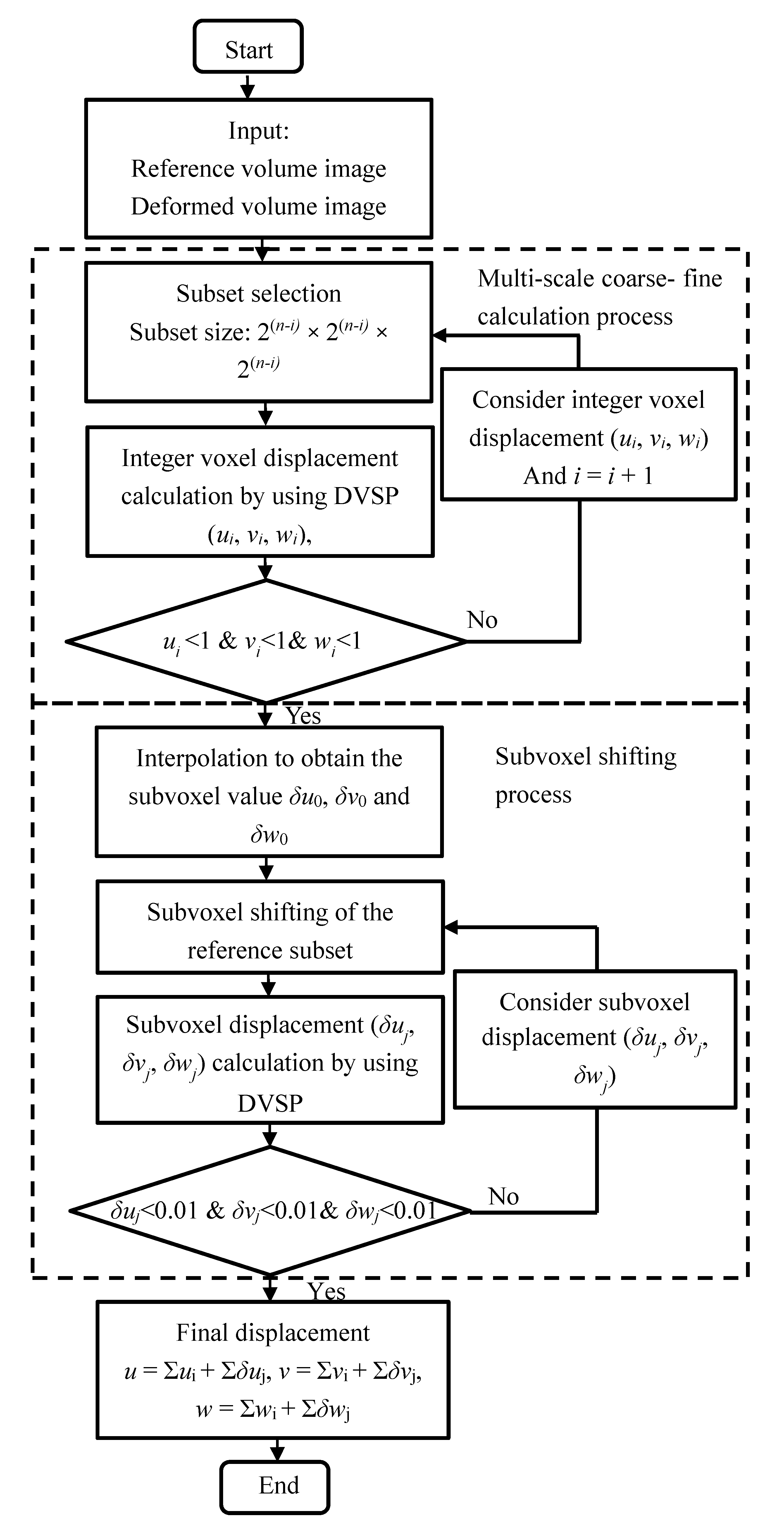
2.1. Theory of Multi-Scale Subset and Subvoxel Shifting in DVSP

The theory of DVSP has been described previously [32] and is only briefly presented here for easy reference. Assume that a reference volumetric image and a deformed volumetric image of an object are acquired by a CT system (i.e., either in nano- or microscale), these two volumetric images are subsequently divided into volumetric subsets with arrays of 16 × 16 × 16 voxels or 32 × 32 × 32 voxels and then ‘compared’. The cross correlation with the POF is operated in the frequency domain (ξ, η, ζ) as follows:

$$\begin{array}{cc}\hfill \overline{G}\left(\xi -u,\eta -v,\zeta -w\right)& =\Im \left\{\frac{H_1\left(f_x,f_y,f_z\right)H_2^{*}\left(f_x,f_y,f_z\right)}{\sqrt{\left|H_1\left(f_x,f_y,f_z\right)H_2\left(f_x,f_y,f_z\right)\right|}}\right\}\hfill \\ & =\Im \left\{\left|H_1\left(f_x,f_y,f_z\right)\right|\exp \left\{j\left[{\varphi }_1\left(f_x,f_y,f_z\right)-{\varphi }_2\left(f_x,f_y,f_z\right)\right]\right\}\right\}\hfill \end{array}$$

(1)

where $\overline{G}\left(\xi -u,\eta -v,\zeta -w\right)$, an expanded impulse function located at (u, v, w), is the discrete 3D cross correlation between the two volumetric subsets. $\Im$ denotes the Fourier transform, with $H_1\left(f_x,f_y,f_z\right)$ being the Fourier transform of $h_1\left(x,y,z\right)$, representing the gray distribution function of a subset from the reference volumetric image, and $H_2\left(f_x,f_y,f_z\right)$ being the Fourier transform of $h_2\left(x,y,z\right)$, representing the gray distribution function of the corresponding subset from the deformed volumetric image. In addition, * denotes the complex conjugate. $\left|H\left(f_x,f_y,f_z\right)\right|$ and $\varphi \left(f_x,f_y,f_z\right)$ are the spectral amplitude and phase fields, respectively.

In Equation (1), the term $\exp \left\{j\left[{\varphi }_1\left(f_x,f_y,f_z\right)-{\varphi }_2\left(f_x,f_y,f_z\right)\right]\right\}$ may be viewed as a POF, which can give a good balance between the peak sharpness and the noise tolerance in the correlation theory. As noted in reference [34], the random error of DVSP depends on subset size and micro structure pattern of objects. Furthermore, if the displacement between the corresponding subsets is large, the increase in the nonoverlapping area would cause an increase in decorrelation and thus result in an enhanced random error. On the other hand, in the case of images, $\overline{G}$ in Equation (1) is only displaying a delta-like function if u, v and w are integers. Non-integer translations between two subsets cause the peak in $\overline{G}$ to spread across neighboring voxels, subsequently degrading the quality of the displacement estimate. To identify sub-voxel investigation, the common approach is to apply cubic spline interpolation. The accuracy of these interpolation methods is highly dependent on the shape of the $\overline{G}$ function near the peak. In the 2D method, a multi-scale and coarse-fine subset calculation process and a subpixel shifting technique have been applied to decrease the error caused by decorrelation and non-integer translations [41,42]. These techniques are hereby introduced into DVSP, and we call this new algorithm Multi-scale and Subvoxel shifting Digital Volumetric Speckle Photography (MS-DVSP).

The essence of the multi-scale and coarse-fine calculation process is to minimize the nonoverlapping area under one voxel. In the coarse calculation process, the largest size of the subset (2ⁿ × 2ⁿ × 2ⁿ) should not be larger than the size of the region-of-interest (ROI) in the reference volumetric image, and the integer voxel of displacement value (u₀, v₀, w₀) is obtained by the DVSP method. After that, the subset with the size (2ⁿ⁻¹ × 2ⁿ⁻¹ × 2ⁿ⁻¹) is applied, the corresponding subset in the deformed volumetric image is re-selected with reference to the first integer voxel predicted displacement (u₀, v₀, w₀), and the displacement value (u₁, v₁, w₁) of each subset is then calculated by the DVSP method. The subset size is gradually reduced according to above mentioned steps. When the subset size reaches a predetermined value and the obtained displacement values Δu, Δv, Δw are no more than 1 voxel in size, then surrounding an integral voxel of the crest a cubic subset with the size of 3 × 3 × 3 voxels is selected and a cubic spline interpolation is used to assess the sub-voxel value δu, δv and δw. The reference subset can be moved with an amount δu, δv and δw by using the shifting property of Fourier transform. To weaken the edge effects and get good localization properties of Fourier transform, the shifted reference subset and the deformed subset are narrowed by a Kaiser window. Then, the subvoxel translation is calculated again. Some errors due to the interpolation require to reiterate by considering the “reference” subset with a new subvoxel shifting until a convergence criterion is matched. The final displacement value (u, v, w) of each subset can be obtained from the sum of the displacement values in the above steps. The flowchart of the MS-DVSP algorithm is shown in Figure 1. The procedures are programmed in MATLAB codes.

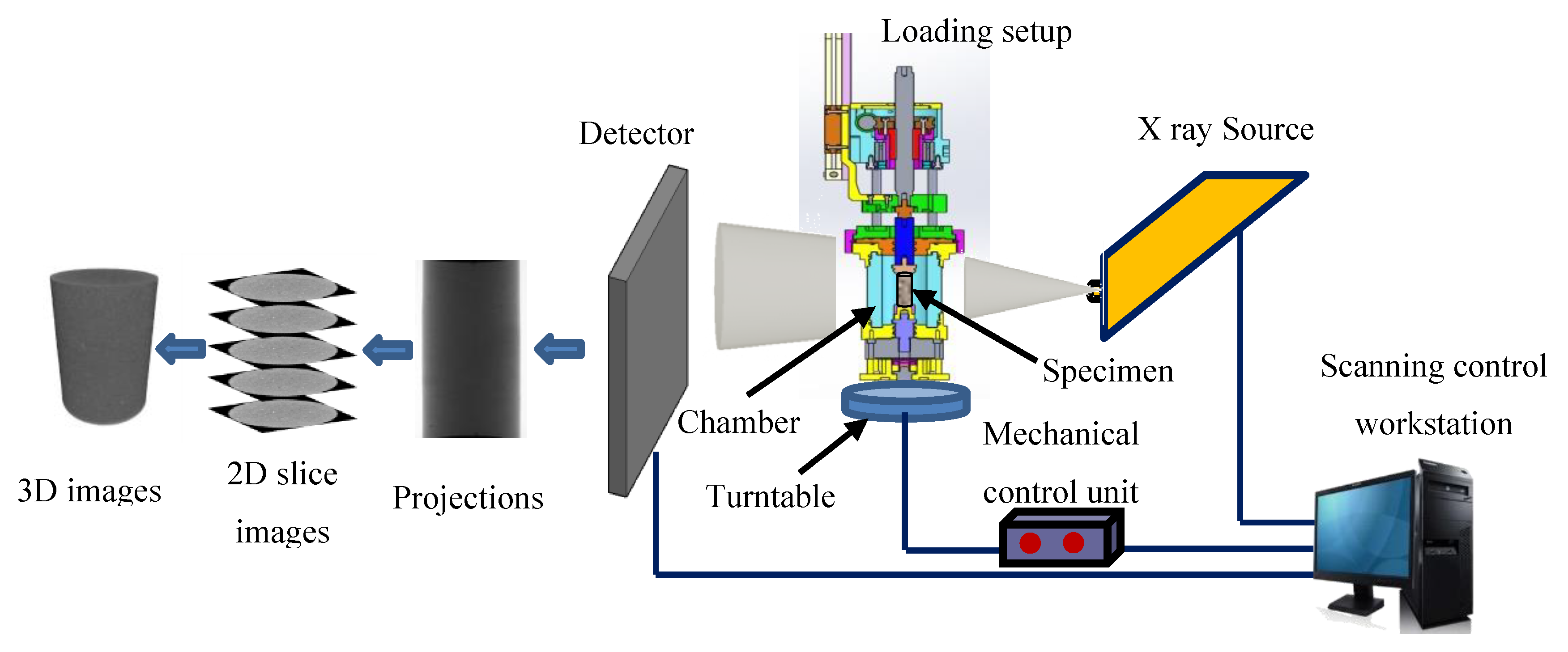
2.2. X-ray Microtomography System and In Situ Loading Setup

The schematic of the X-ray microtomography system and a custom-made in situ loading setup is illustrated in Figure 2. The X-ray microtomography system mainly consists of a FXE 225 kV micro focus X-ray source from YXLON (Hamburg, Germany), an array detector (XRD 0822 AP14, Varex Imaging Corporation, Salt Lake City, UT, USA) of dimensions 1024 × 1024 pixels from PerkinElmer (Waltham, MA, USA), a turntable and its mechanical control unit, and a scanning control workstation [39]. The custom-made in situ loading setup is mounted on the turntable by using bolts, and rotates 360° with the turntable. In the loading experiment, the specimen is placed on the stage in the Poly(methyl methacrylate) (PMMA) chamber of the setup, and the mechanical loading is controlled by an electric motor. While the specimen is rotating step by step over 360°, a set of 720 radiograph projections are captured. When each projection is captured, the turntable does not move. It takes about 25 min for one 360° scan. After that, a Feldkamp cone-beam algorithm is used to reconstruct a sequence of 2D 16-bit slice gray images [43]. Based on these slice images, a 3D image is obtained.

3. Experiment and Results

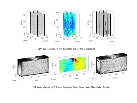
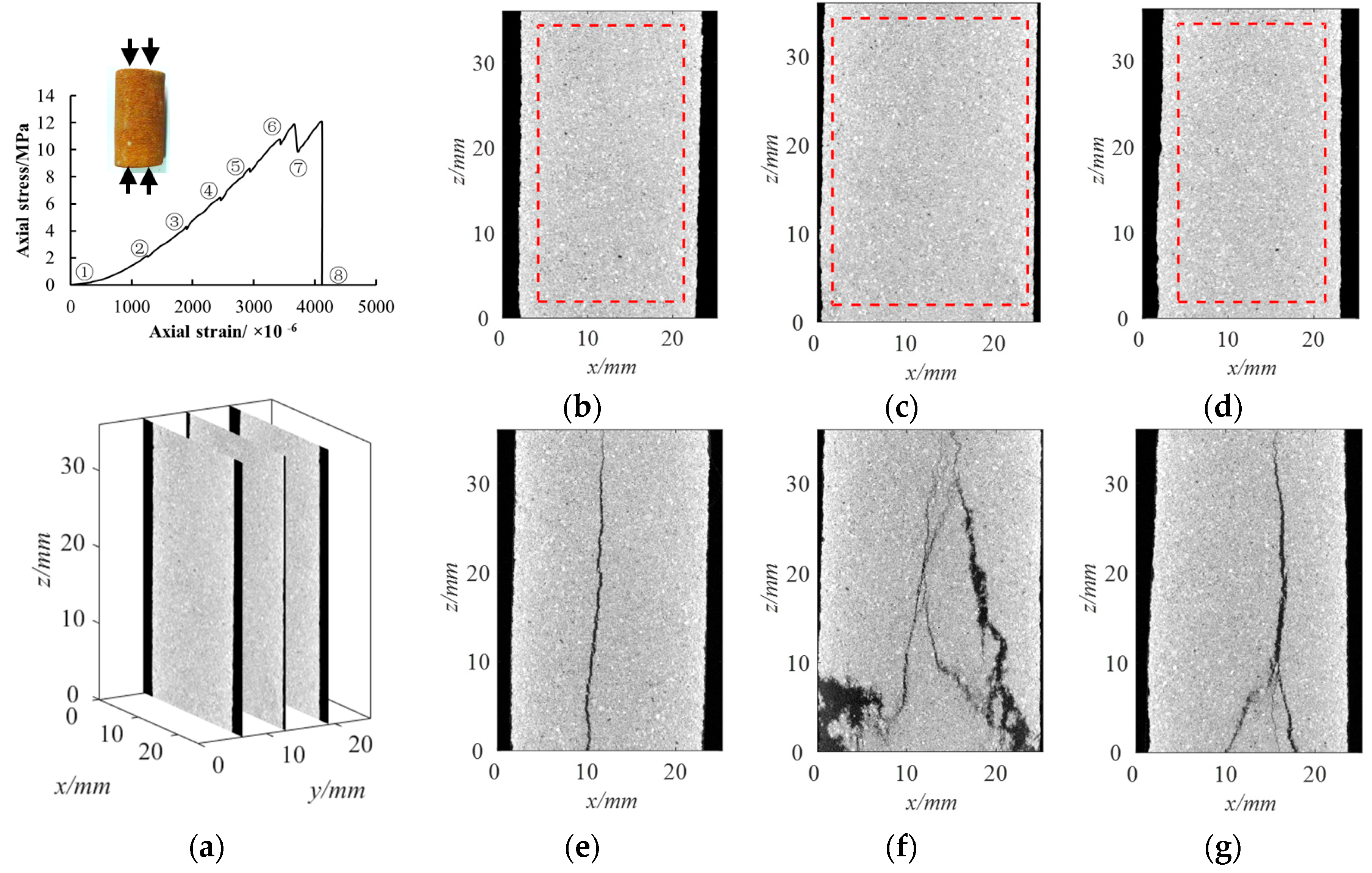
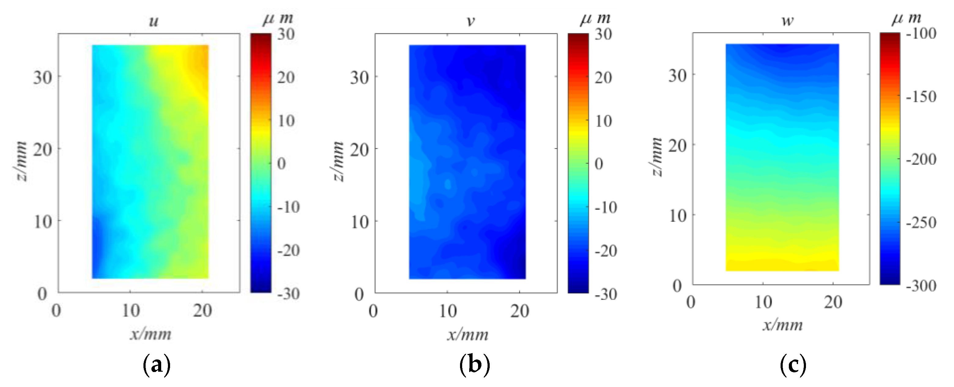
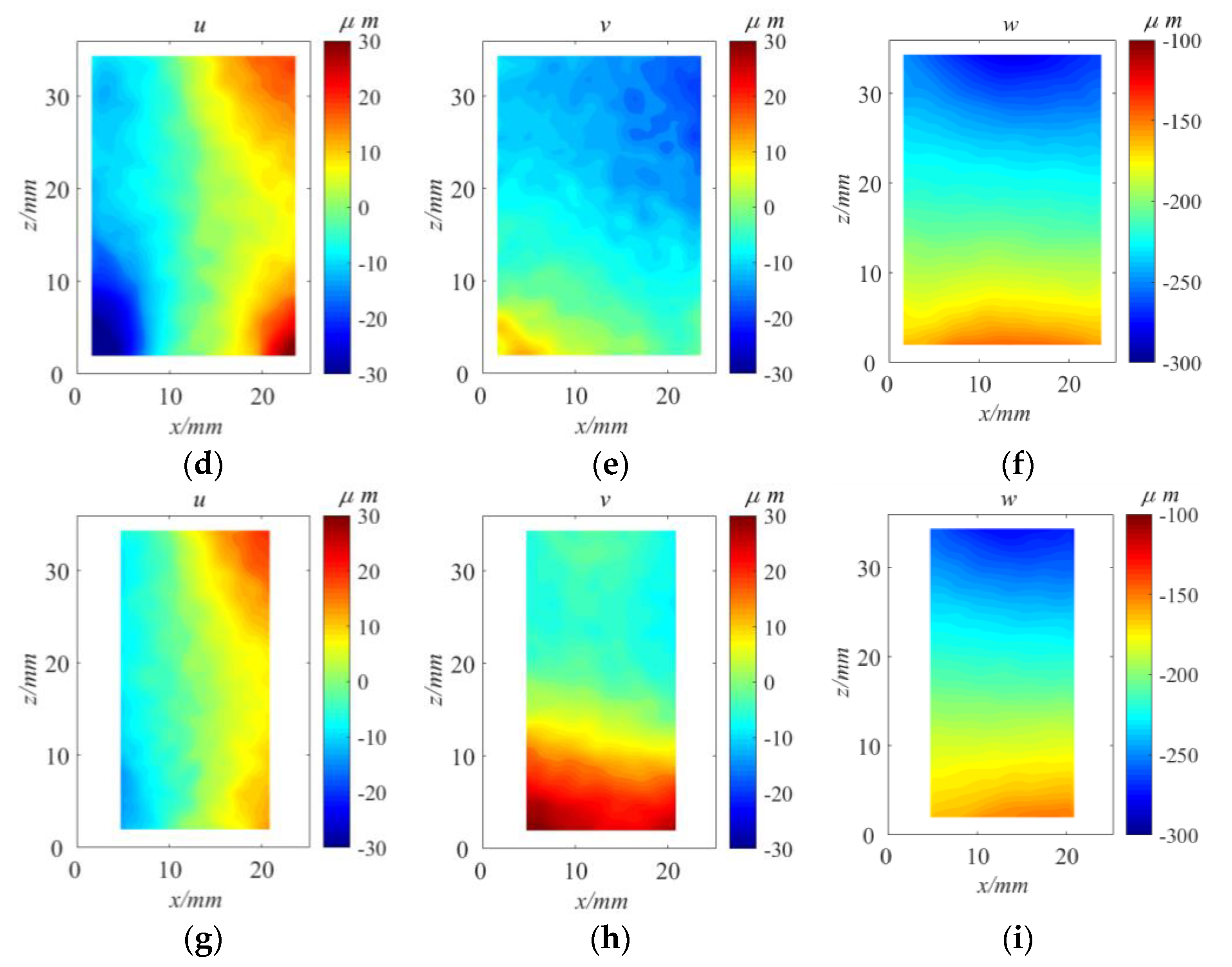
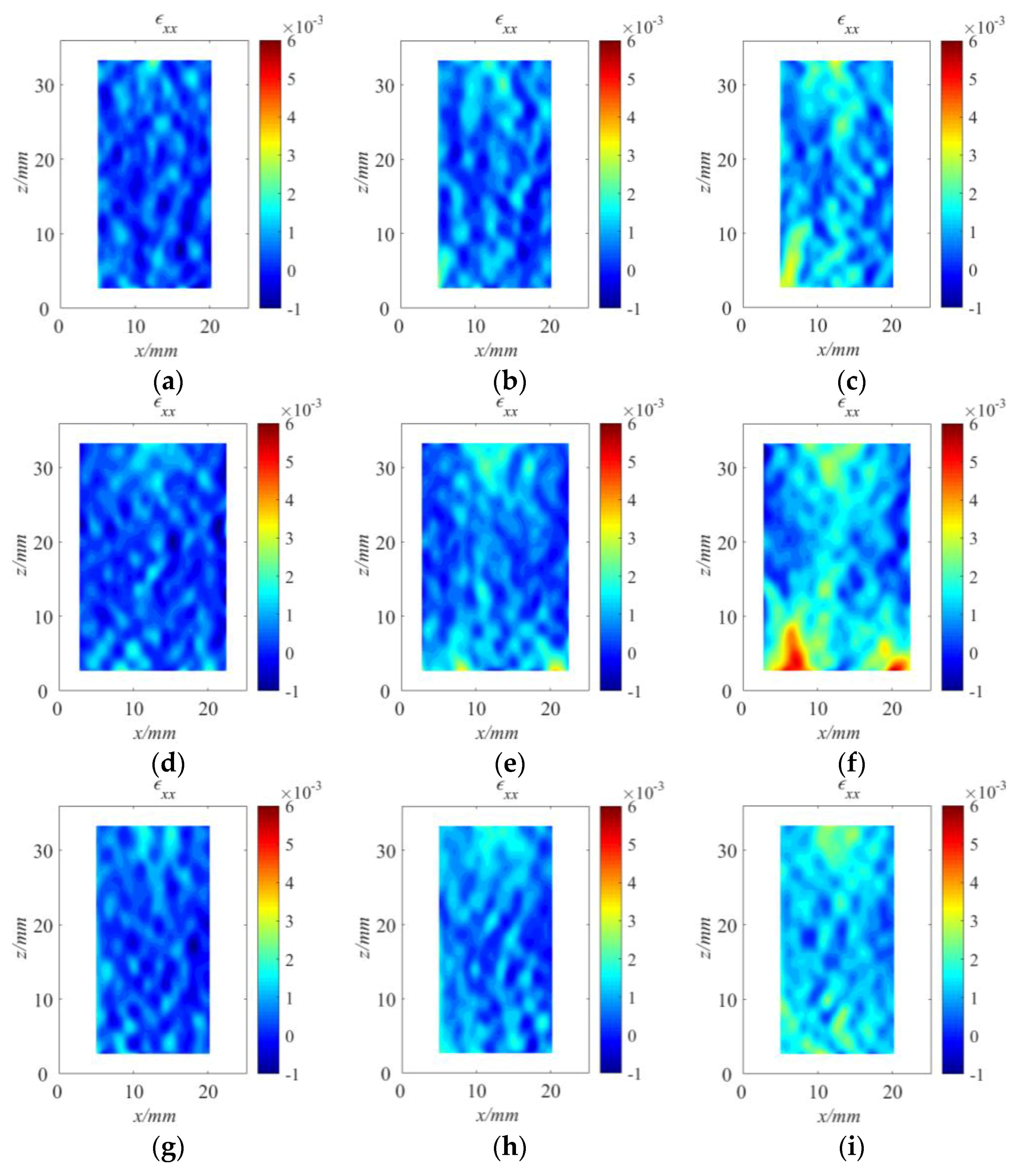
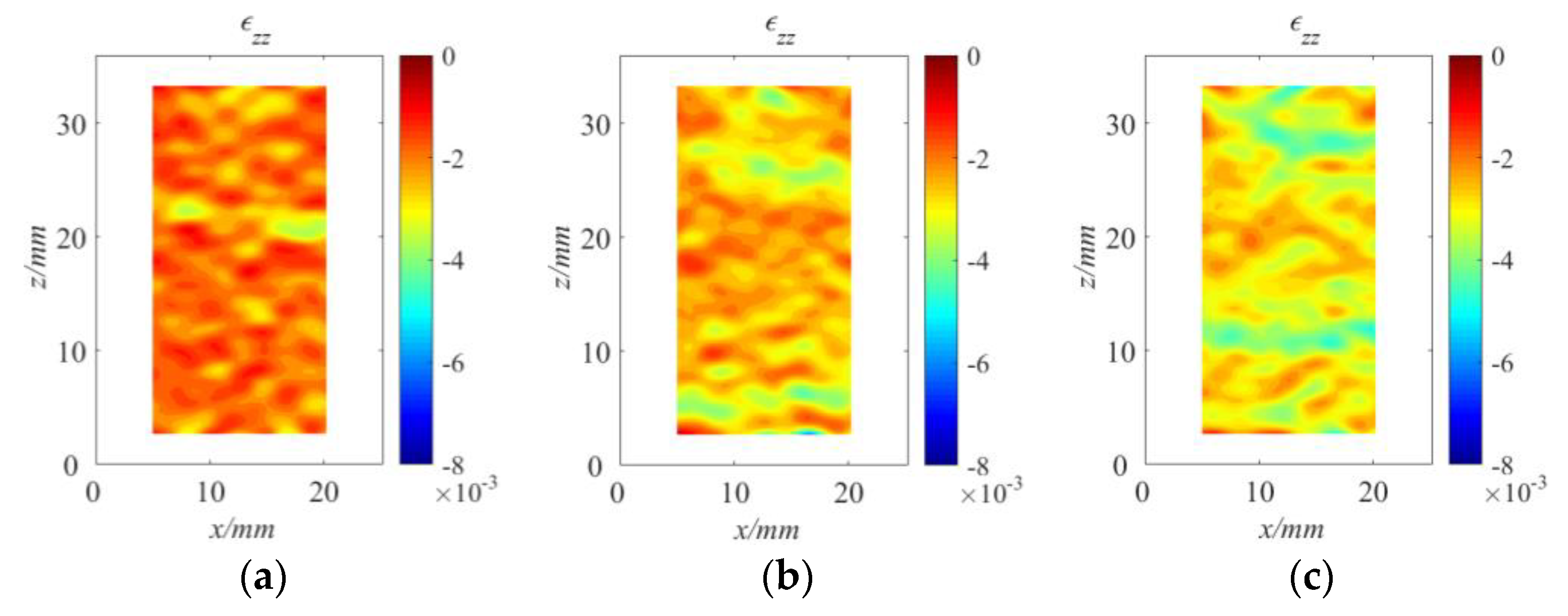
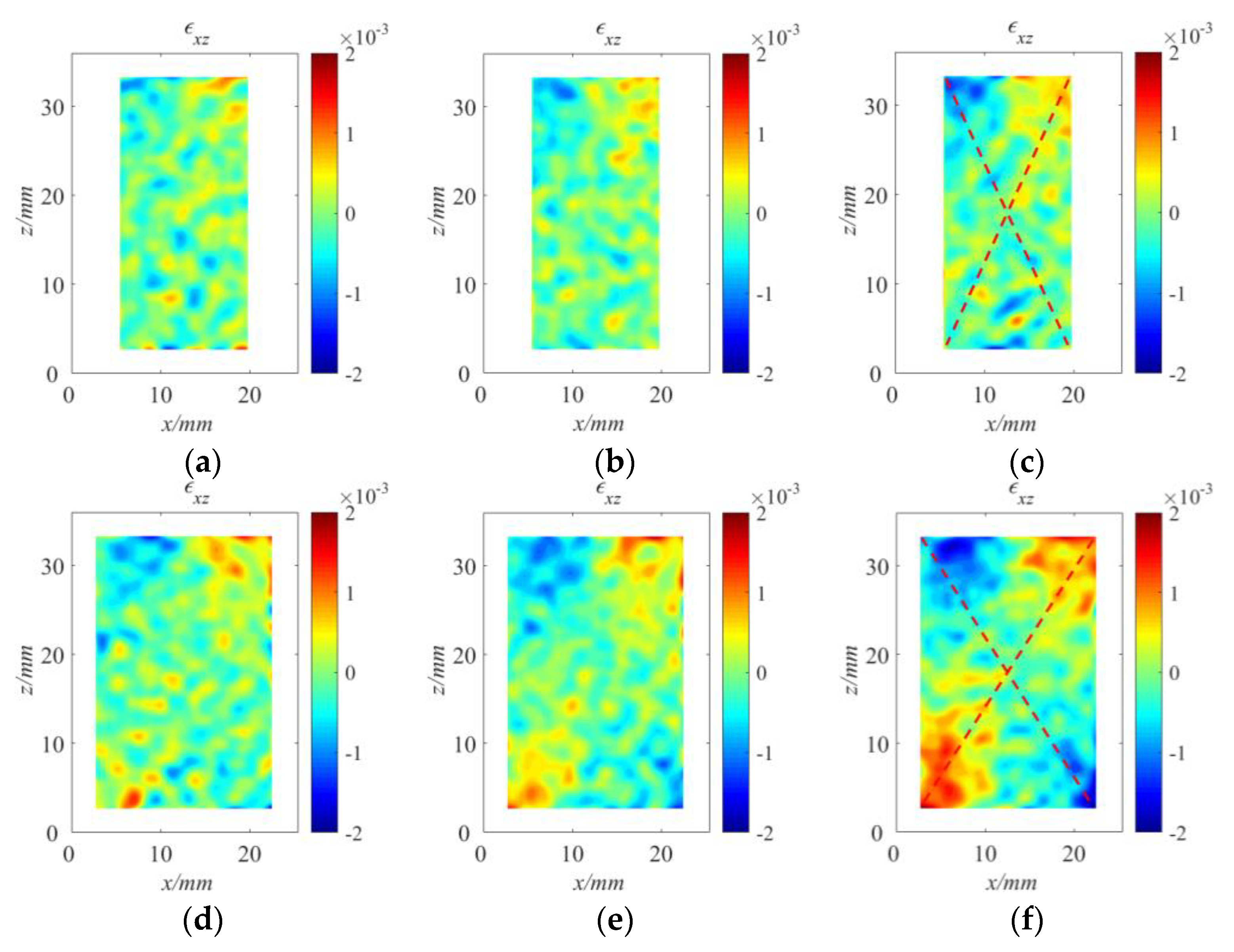
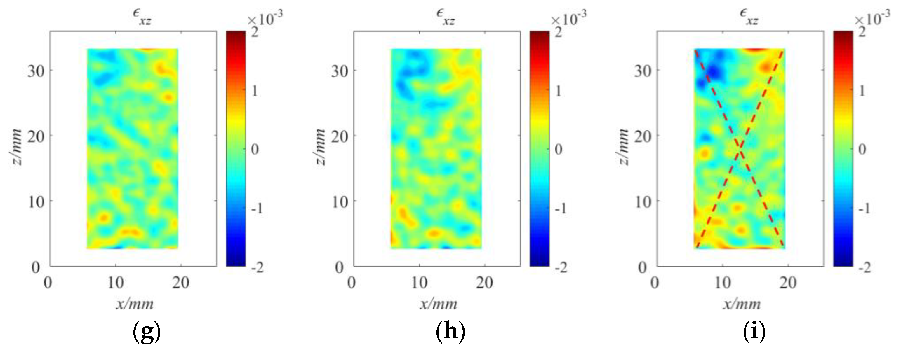
3.1. Internal Strain Investigation of Red Sandstone Exposed to Compression

A cylindrical specimen of red sandstone of 25 mm in diameter and 50 mm in length is scanned under different compression loadings in situ. The scan voltage is 120 kV, and the current is 200 μA. The experimental process is divided into 8 steps as shown in the stress–strain curve in Figure 3a. In each step, the specimen is scanned when the force is stable. In step 1, we take two consecutive scans of the specimen in identical settings and without moving (except the tomographic rotation) or deforming the specimen and designate them as Scans 1 and 2, respectively. Those two scans are used to evaluate artifacts and image noise influences in Section 4.2. In step 7, the loading value decreases due to the development of micro cracks, but the specimen still has loading capacity till the loading reaches the peak value of 12.08 MPa. In step 8, the broken specimen is scanned. In Figure 3, three sectional images at y = 6.20 mm, 12.50 mm and 18.80 mm of the specimen in step 6 and step 8 are shown, respectively. From the gray images shown Figure 3b–d, it is difficult to ascertain the damage. With reference to Figure 3e–h, the coalescence of tensile cracks mainly results in the failure of the specimen. At the lower left and right corners of the middle sectional image shown in Figure 3f, there are also some cracks due to shear stress. We select the volumetric image of step 1 as the reference image, and volumetric images of other steps as the deformed images, respectively. The size of the volumetric image has 560 × 560 × 801 voxels and the dimension of a unit voxel is 45 μm × 45 μm × 45 μm. By using the MS-DVSP algorithm, displacement fields are calculated. The final subset size is 32 × 32 × 32 voxels and the shift of the subset is 10 voxels. The calculated region of each section is the rectangular area marked with the dashed lines in Figure 3b–d. The u, v and w displacement fields of all sectional images of step 6 are plotted in Figure 4. As expected, the specimen mainly bore compression deformation along the z axis, and maximum displacements exist in the top region. Illustrated in Figure 4a,d,g, displacement fields of sectional images are divided into the negative and positive displacement regions, which make the specimen tensile along x axis. The main cracks shown in Figure 3e–h can be predicated by the zero displacement interface. This tensile deformation can also be investigated along y axis. In Figure 4b,e,h, the displacement of the sectional image at y = 6.20 mm is negative, while the displacement of most area of the sectional image at y = 18.80 mm is over zeros, especially in the lower region. These displacement distribution characteristics manifest that the expansion deformation occurs in circumference.

Strain estimation can be derived from computed displacement fields by using numerical computation methods. During this procedure, the noise in computed displacement fields will result in decreasing the reliability of strain estimation. It is necessary to smoothing the calculated displacement dataset before strain estimation [44]. Here, we first apply multivariate kernel smoothing regression [45] to smooth the displacement fields. After that, a point-wise least-squares (PLS) [46] approach is used to compute the internal strain fields. The size of the strain calculation cubic element is 33 × 33 × 33 voxels, and the distance between the center points of the neighbor element is 10 voxels. The normal strains and shear strains of these sections in step 4, 5 and 6 are plotted as shown in Figure 5, Figure 6 and Figure 7, respectively. Here, in normal strain, we define positive corresponding to tension and negative corresponding to compression. From normal strain contours ε_xx shown in Figure 5, with the loading increase, it is noted that the deformation localization first occurs in both ends of the specimen, and develop to the middle. These localization regions correspond to the main cracks shown in Figure 3e–h. The distributions of normal strain ε_zz (shown in Figure 6) indicate that the compression deformation along the axis z is nearly uniform under small loading. With loading increase, deformations in both ends grow up more than ones in the middle. The maximum compression strain occurs at the bottom of the specimen. Due to friction among the specimen and two compression plates, the distributions of shear strain ε_xz take the shape of an ‘x’, as marked by the dashed lines in Figure 7, which depicts the characteristics of the shear deformations in the specimen. It is the shear deformation (shown in Figure 7f) cooperating with tensile deformation (shown in Figure 5f) that lead to the damage at the lower left and right corners of the specimen. These strain contours are useful in our efforts to understand the failure mechanism of the material.

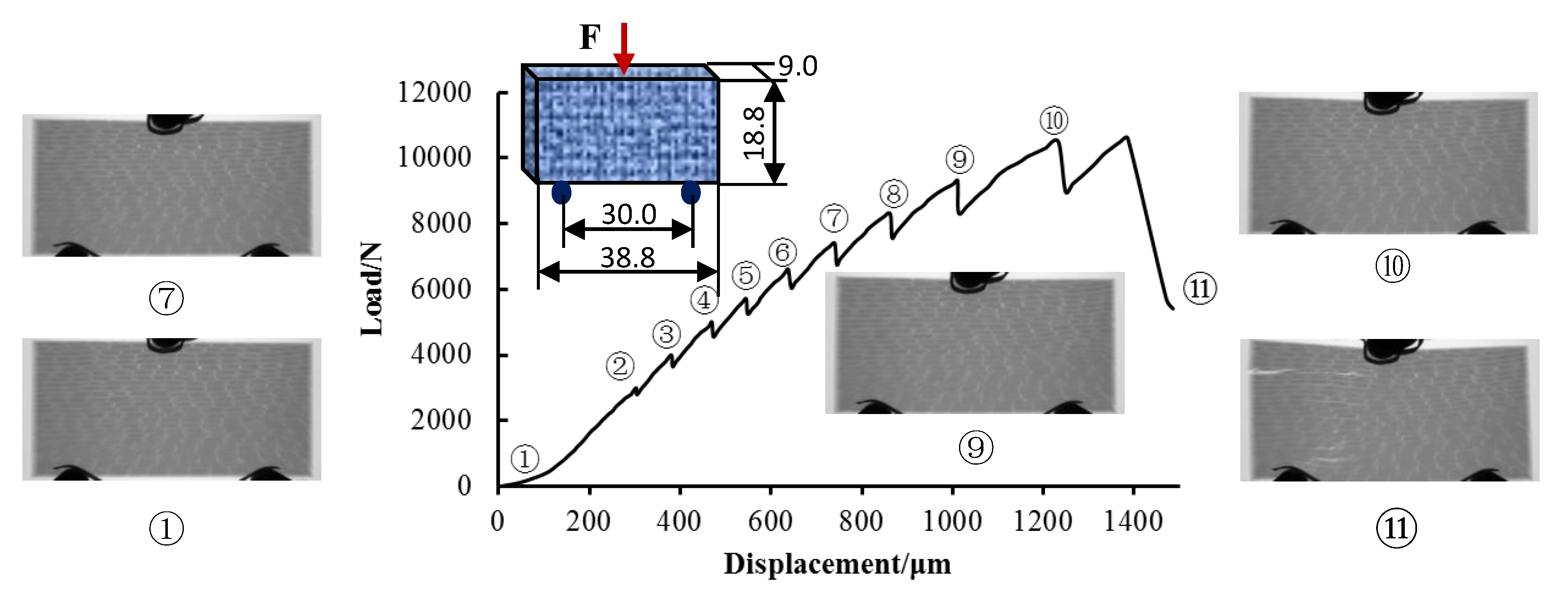
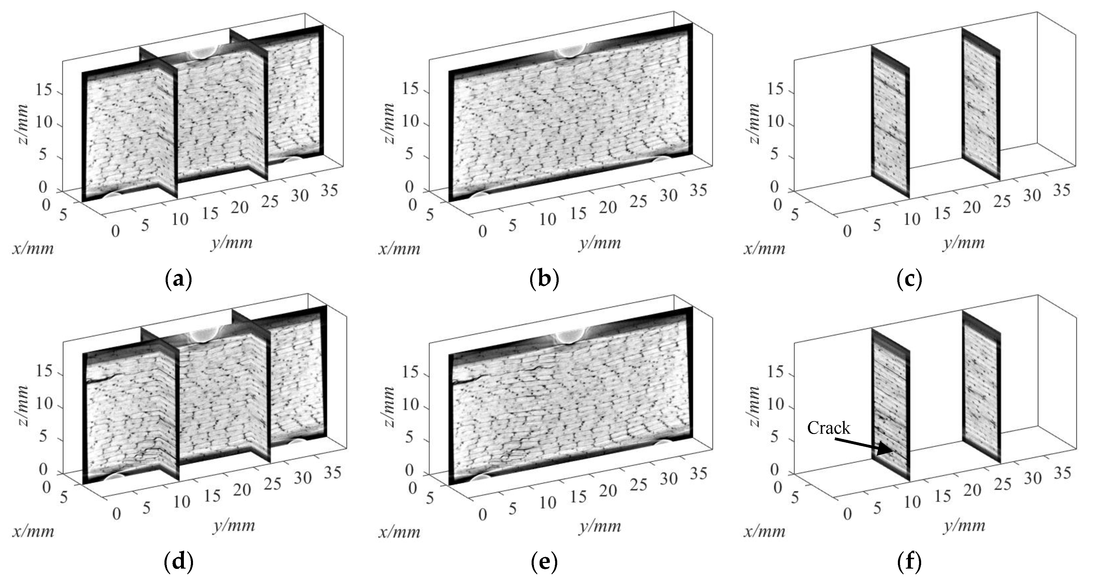
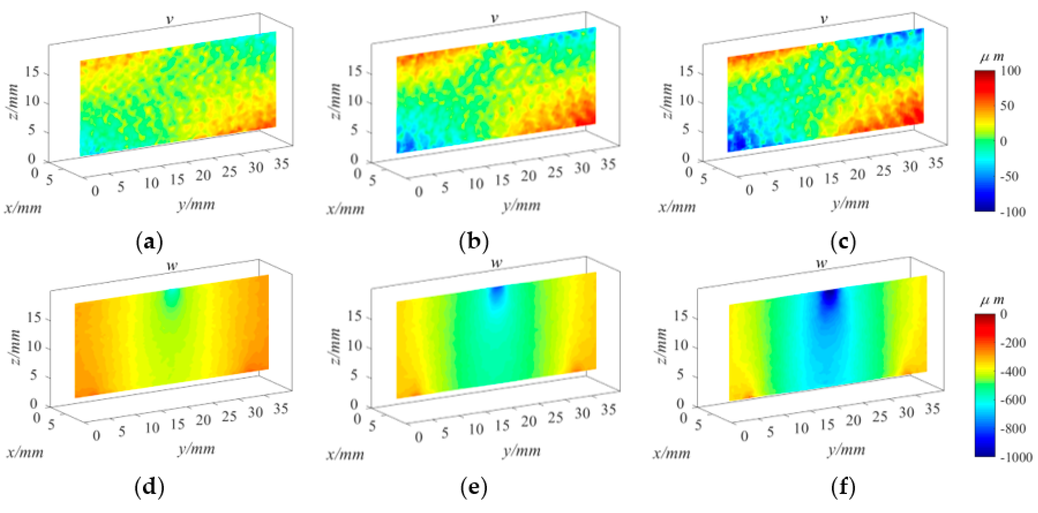
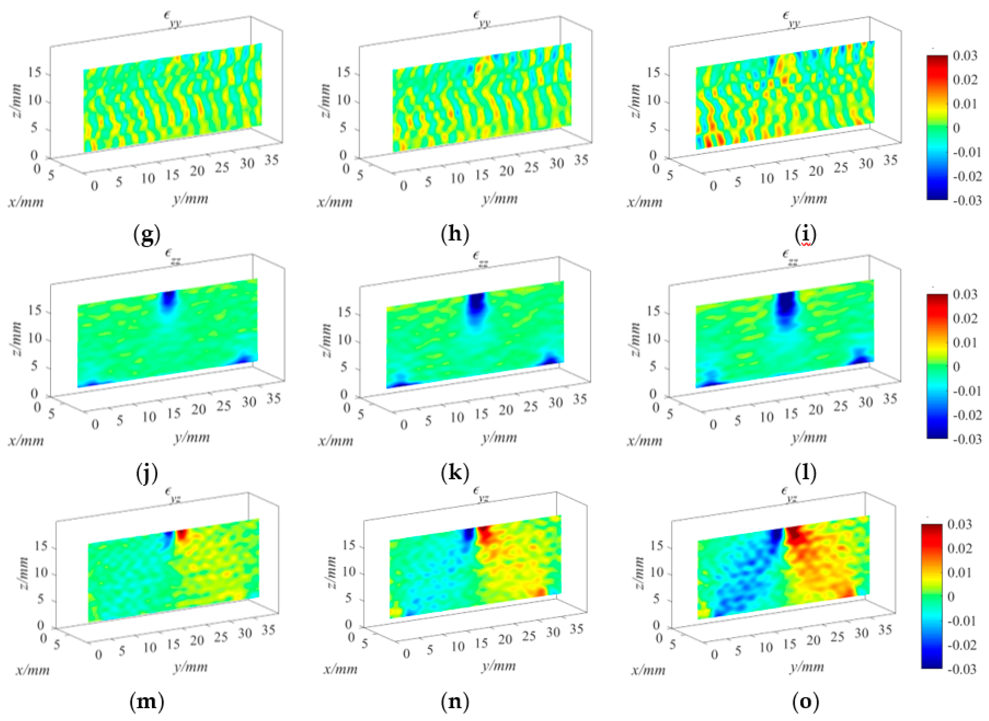
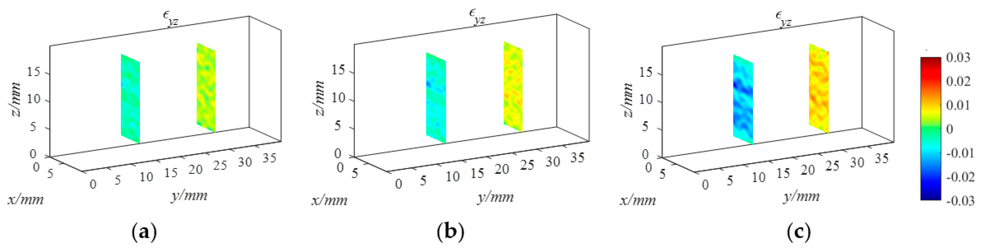
3.2. A Woven Composite Short Beam Under Three-Point Bending

A short woven composite short beam under three-point bending experiment has been described in reference [37,39]. The load-displacement curve is plotted in Figure 8, and Figure 11 scan steps are marked on the curve. The scan voltage is 130 kV, and the current is 200 μA. Five radiography projections are shown in Figure 8. The areas with high gray value correspond to pores in the specimen. From those projections before step 11, no much more damage information can be detected. In the projection of step 11, the specimen is broken, more areas with high gray value occur among layers on the left side of the specimen, which correspond to the cracks among layers. A 3D image of 900 × 250 × 361 voxels is reconstructed in each scan step, and a unit voxel is 45 μm × 45 μm × 45 μm. Limited by the CT system resolution, fibers can not be distinguished from the matrix. The middle longitudinal sectional image and two transverse sectional images of the 10th scanning step are shown in Figure 9a–c, respectively. Pores have low gray value, which inverses to the projection. No discernable cracks are detected from these gray images. In the 11th scanning step, delamination and cracks are clearly visible on the left side of the specimen from the upper loading point to the bottom support shown in Figure 9e. We recalculate the internal displacement and strain fields with the MS-DVSP algorithm and the PLS approach, respectively. Due to heterogeneity in structures, we select the final subset size of 32 × 32 × 32 voxels and the subset shift of 5 voxels to obtain much more displacement detail.

In Figure 10, v, w displacement fields and ε_yy, ε_zz and ε_yz strain fields of the middle longitudinal sectional image at step 7 (F = 6761 N), step 9 (F = 8333 N), and step 10 (F = 8982 N) are depicted, respectively. v, w displacement distributions are consistent to typical patterns of a short beam under three-point bending, but the periodic distribution of the internal structure in the woven composite specimen makes v displacement show periodic fluctuation in the longitudinal direction, which also be manifested by ε_yy strain distribution shown as Figure 10g–i. From ε_zz strain distribution illustrated in Figure 10j–l, the periodic fluctuation in the transverse direction is due to the layer structure of the specimen. From the contours of the shear strain ε_yz, the strain growth in regions from the loading point to two supports is evident with loading increase, and the high strain value is the prelude to the eventual delamination failure as shown in Figure 9e at Step 11. ε_yz strain fields of two transverse sectional images are depicted in Figure 11. Before the specimen is broken, it is also found that high strain occurs on the region which corresponds to the crack area shown in Figure 10f.

4. Discussion

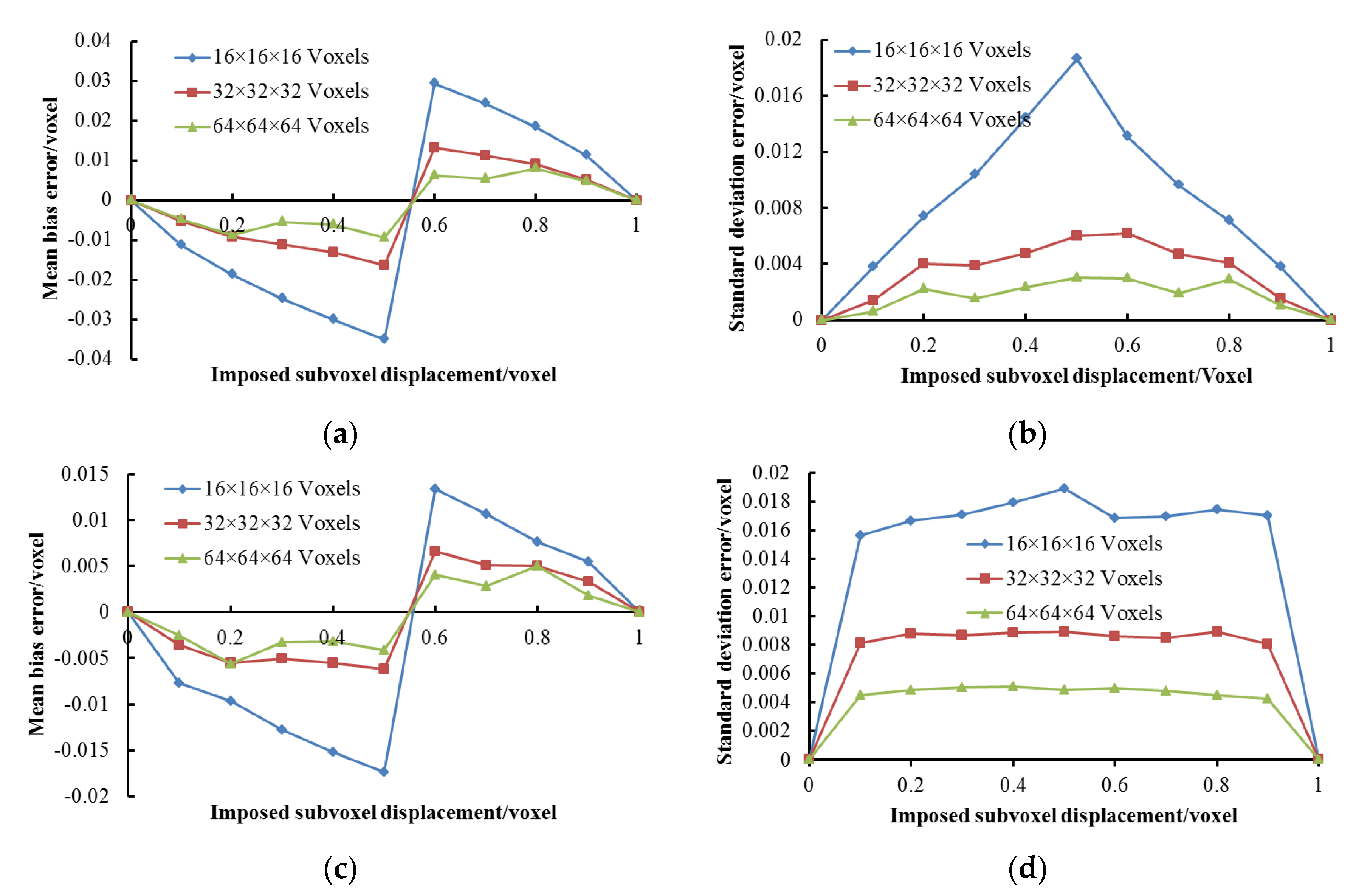
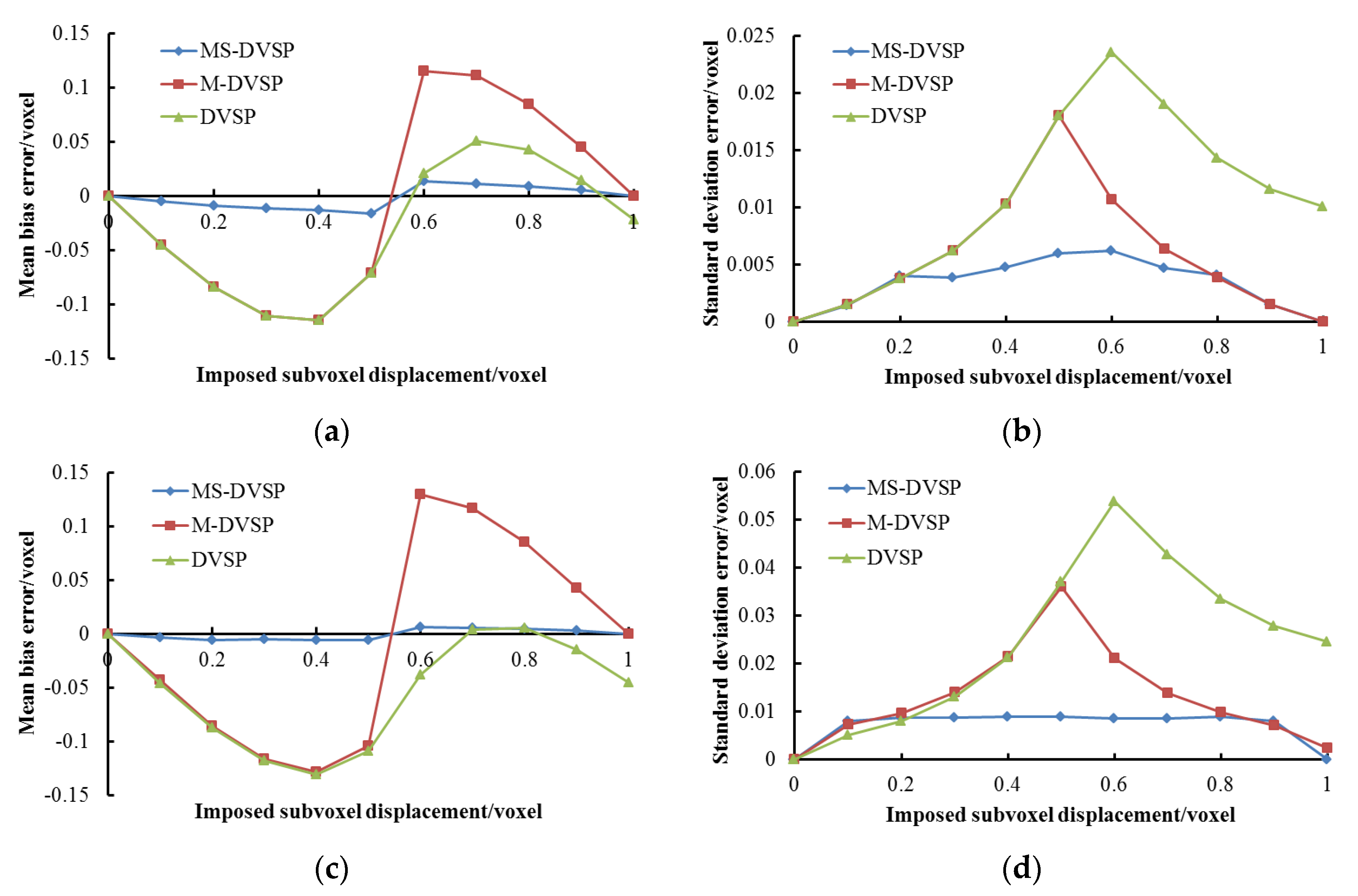
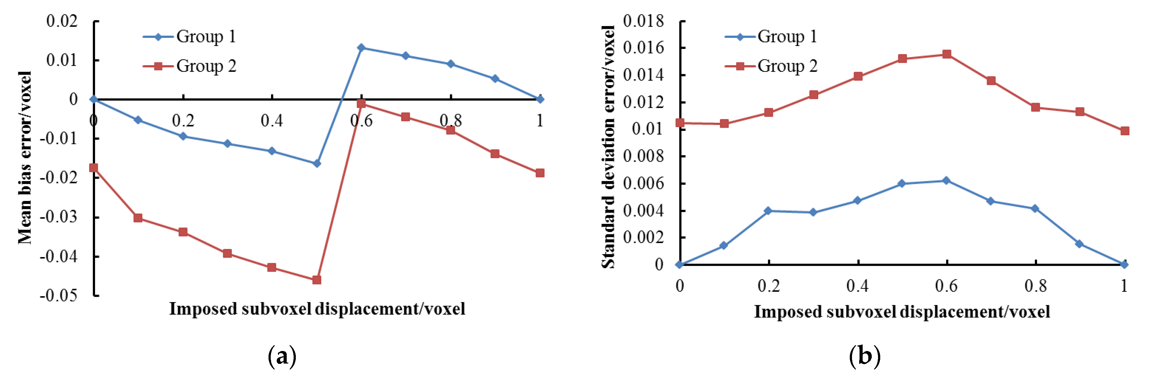
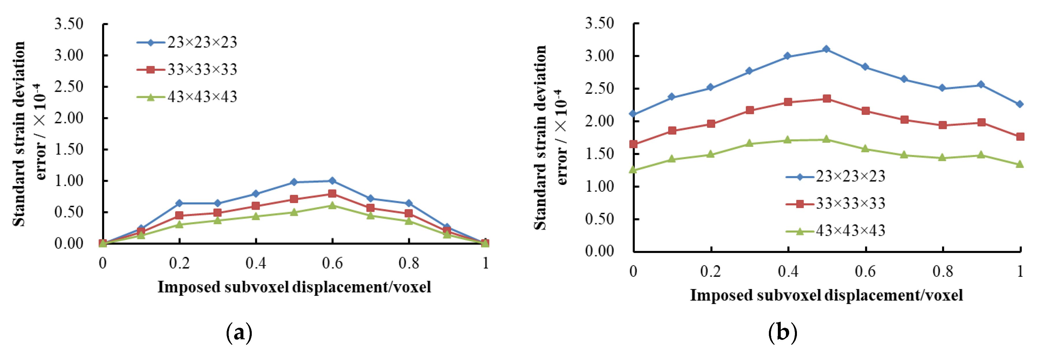
4.1. Assessment of Accuracy of MS DVSP

For evaluating the robustness of an algorithm, numerical experiments are usually used. There are two methods to generate the reference and the deformed images. The first method is to apply computer simulation to digitally generating images. This method can isolate the possible errors caused by the image acquisition. In most DVC and DVSP applications, natural microstructures are seen as the speckle patterns. It is difficult to find a mathematic function to describe and simulate the natural microstructures. The second method is to employ the original image of a specimen as the reference image, and the deformed images can be generated by using synthetic shifts with Fourier transform. In this paper we use the second method. Two volumetric images of 200 × 200 × 200 voxels are isolated from the reconstructed images of step 1 in the above two experiments, which are defined as the reference images, respectively. The “deformed” volumetric images are generated by imposing a rigid displacement ranging from 0.1 to 1.0 voxel with an increment of 0.1 voxel along the z direction. By using the MS-DVSP algorithm, pre-imposed sub-voxel translation displacements are calculated. The predetermined subset sizes are defined as 16 × 16 × 16 voxels, 32 × 32 × 32 voxels and 64 × 64 × 64 voxels, respectively, and the shift of the subset is 10 voxels. Figure 12 shows both the mean bias error and the standard deviation error as a function of the imposed displacement for different subset sizes. With a predetermined subset size, the error reaches maximum at 0.5 voxels. In this situation the information between each subset in the reference and deformed images is the most biased. Furthermore the larger is the subset, the smaller the error. But, increasing the subset size would degrade the spatial resolution. We define the predetermined subset size as having 32 × 32 × 32 voxels. With this subset size the maximum mean bias error of the red sandstone specimen is 0.0160 voxels and the corresponding standard deviation error is and 0.0060. For the woven composite specimen, the maximum mean bias error is 0.0062 voxels, and the corresponding standard deviation error is and 0.0089 voxels. The difference of accuracy between those two materials depends on their natural structures. The Shannon entropy values [47] of the red sandstone and the woven composite are 2.7606 and 3.0337, respectively, which means the woven composite has more feature information seen as speckle patterns resulting in a bit higher accuracy in the measurement.

In reference [39] a multi-scale coarse-fine subset calculation process was used in DVSP, which also increased the performance of DVSP. We call this algorithm M-DVSP. To compare the performance of MS-DVSP, M-DVSP, and DVSP, we calculate the displacements of these volumetric images with imposed sub-voxel translation using these three algorithms, respectively. The subset size is predetermined at 32 × 32 × 32 voxels, and the shift of the subset is 10 voxels. The error curves are plotted as shown in Figure 13. The performance of M-DVSP algorithm is slightly better than that of DVSP, especially in standard deviation errors after 0.5 voxels. When the imposed displacement is increased continuously, the overlapping area between the reference subset and the deformed subset is decreased, and the noise caused by non-overlapping becomes stronger. As a result, it can be expected that the errors of DVSP will get progressively worse. Among these three algorithms, the performance of MS-DVSP is the best. Based on the mean bias error and its corresponding standard deviation error, we can find that the maximum error of the red sandstone specimen is 0.022 voxels of the MS-DVSP algorithm, 0.125 voxels of M-DVSP algorithm, and 0.124 of DVSP algorithm. The maximum error of MS-DVSP is only about one sixth of those errors of the other two algorithms, DVSP and M-DVSP. In the case of the woven composite specimen, the maximum errors are as follows: 0.015 voxels of the MS-DVSP algorithm, 0.150 voxels of the M-DVSP algorithm, and 0.151 of the DVSP algorithm. Thus, the maximum error of MS-DVSP is only about one tenth of those errors of the other two algorithms. These results indicate that MS-DVSP algorithm is an effective way to increase the accuracy of the technique, and the performance of MS-DVSP also depends on the internal micro-structures of objects.

4.2. Influence of Artifacts in CT Image

During reconstruction of CT slice image, the non-uniformity of detector units and the polychromatic nature of the X-ray will give rise to ring and beam hardening artifacts. The self-heating effect of X-ray tube may result in distance variations that induce magnification changes and thus spurious dilatational strain. In addition, the image noise and contrast, the imperfect motion of the rotation stage, and the possible rigid body motion of the specimen will all influence the measurement result. Among all these effects, the spurious dilatational strain is definitely the most important to correct. More detailed information on the influence of these effects can be found in references [48,49,50,51]. Here, we just discuss the influence of the image noise and the imperfect motion.

To analyze the effect of artifacts of the micro X-ray CT system on the MS-DVSP algorithm, we take two consecutive scans in step 1 of the red sandstone specimen in Section 3.1 as the baseline experiment. Noise and artifacts of the system are included in the reconstructed images. For saving the computation time, we isolate two volumetric images having 200 × 200 × 200 voxels from the center of reconstructed images of Scan 1 and Scan 2, define them as the reference image and the deformed image, respectively, and calculate displacements by using the MS-DVSP algorithm. The predetermined subset size is 32 × 32 × 32 voxels, and the shift of the subset is 10 voxels. The average measured displacements are u = −0.0059 voxels, v = −0.0147 voxels, and w = 0.0175 voxels, and the standard deviation errors are 0.0107 voxels, 0.0115 voxels and 0.0105 voxels, respectively. The measured displacement along y and z axes is greater than the standard deviation error, indicating that some motion occurred along y and z axes between these two scans due to physical perturbations in the CT system. Because there are real noise and artifacts in the volumetric images of Scans 1 and 2, the above results indicate that the uncertainty of displacement measurement in all three directions is about 0.02 voxels with the MS-DVSP algorithm in the red sandstone specimen experiment.

For investigating the influence of noise and artifacts, two groups of deformed volumetric images are obtained by imposing subvoxel displacements on above two cropped volumetric images, and they are marked as Group 1, and Group 2, respectively. We define the cropped volumetric image of Scan 1 as the reference image, and the images of Group 1 and Group 2 as the deformed images, respectively. Then we calculate the displacements with the MS-DVSP algorithm. The predetermined subset size is 32 × 32 × 32 voxels, and the shift of the subset is 10 voxels. Figure 14 illuminates the results of the displacement measurement. Due to the influence of noises and artifacts, the error increases almost two times. The uncertainty of displacement measurement is 0.015 voxel.

As a more accurate alternative to fitting just rigid body movements, a least squares fit is used to calculate the rigid body translations and rotations, assuming small angles [52],

$$\begin{array}{l}{u}_{rigid}+{\theta }_{z}Y-{\theta }_{y}Z\cong U\\ v_{rigid}-{\theta }_{z}X+{\theta }_{x}Z\cong V\\ w_{rigid}+{\theta }_{y}X-{\theta }_{x}Y\cong W\end{array}$$

(2)

where θ_x, θ_y, and θ_z are the rotations about the x, y, and z axes, respectively, and X, Y, Z and U, V, W are the vectors of the x, y, z coordinates and u, v, w displacements, respectively, for all of the correlation points. The rigid body displacements are u_rigid = −0.0082 voxels, v_rigid = −0.0204 voxels and w_rigid = 0.0167 voxels, and the rotations are θ_x = 2.13×10⁻⁵, θ_y = −3.15 × 10⁻⁵ and θ_z = 3.43 × 10⁻⁵. There are rigid body translations similar to the average measured displacements. Thus, when compared with the volumetric image of Scan 1, the volumetric image of Scan 2 incur very small rigid body translation and small rotation in all three directions. Compared with the deformation of the specimen in our study, the rigid body translation and rotation are very small, so we neglect the influence of the imperfect motion of the rotation stage in the data analysis.

To assess the uncertainty of strain measurement, we use the above calculated imposed subvoxel displacement results to compute strains with the PLS approach. Three sizes of strain calculation cubic box surrounding the point of interest are used, and they are 23 × 23 × 23 voxels, 33 × 33 × 33 voxels and 43 × 43 × 43 voxels, respectively. Since only a rigid body translation is imposed, strains should be zero. However errors of displacement fields give rise to the error of strain calculation. The standard deviation errors of ε_zz is shown in Figure 15, which dictates that the uncertainty of strain measurement depends on the size of the calculation box, the larger is the box, the smaller the uncertainty. In PLS approach, too small calculation box is not enough to smooth the noise existing in local displacement fields, making strains having large variation. On the contrary, too large calculation box may result in local displacement fields oversmoothed. It is suggested that the size of the calculation box can be equal to or slightly larger than the size of the reference subset [46]. So in this study, we select the calculation box of 33 × 33 × 33 voxels. With this size, the uncertainty of strain measurement increases more than two times due to the influence of noise and artifacts, and it is 2.34 × 10⁻⁴.

5. Conclusions

This paper presents an improved algorithm called MS-DVSP to enhance the accuracy of the DVSP technique. The improvement in the algorithm lies in the fact that the two subsets that are correlated are shifted by nonintegral voxel values to obtain a maximum overlap between them. We tested the proposed scheme on red sandstone and woven composite specimens. Compared with DVSP, the accuracy and precision of MS-DVSP increase remarkably. In this study, with consideration of artifacts and noise in CT images, uncertainties of the displacement measurement and the strain measurement of the red sandstone specimen by using MS-DVSP algorithm, are 0.015 voxels and 2.34 × 10⁻⁴, respectively.

The interior displacement and strain fields in a red sandstone specimen under compression and a woven composite specimen under 3-point bending are mapped using the MS-DVSP algorithm. From these plots, the characteristics of the interior deformation of the specimen are clearly depicted, thus elucidating the failure mechanism of the material. We believe the MS-DVSP algorithm will contribute to the further understanding of the physics and mechanics of opaque materials under stress.

References

1. Burch, J.M.; Tokarski, J.M.J. Production of multiple beam fringes from photographic scatters. Opt. Acta 1968, 15, 101–111. [Google Scholar] [CrossRef]
2. Leendertz, J.A. Interferometric displacement measurements on scattering surface utilizing speckle effect. J. Phys. E 1970, 3, 214–218. [Google Scholar] [CrossRef]
3. Chiang, F.P.; Asundi, A. White light speckle method of experimental strain analysis. Appl. Opt. 1979, 18, 409–411. [Google Scholar] [CrossRef] [PubMed]
4. Chiang, F.P.; Jin, F. A new technique using digital speckle correlation for nondestructive inspection of corrosion. Mater. Eval. 1997, 55, 813–816. [Google Scholar]
5. Chen, D.J.; Chiang, F.P. Computer-aided speckle interferometry using spectral amplitude fringes. Appl. Opt. 1993, 32, 225–236. [Google Scholar] [CrossRef] [PubMed]
6. Chen, D.J.; Chiang, F.P.; Tan, Y.S.; Don, H.S. Digital speckle-displacement measurement using a complex spectrum method. Appl. Opt. 1993, 32, 1839–1849. [Google Scholar] [CrossRef] [PubMed]
7. Chiang, F.P.; Asundi, A. Interior displacement and strain measurement using white light speckles. Appl. Opt. 1980, 19, 2254–2256. [Google Scholar]
8. Burguete, R.L.; Patterson, E.A. A photoelastic study of contact between a cylinder and a half-space. Exp. Mech. 1997, 37, 314–323. [Google Scholar] [CrossRef]
9. Ju, Y.; Xie, H.P.; Zheng, Z.M.; Lu, J.B.; Mao, L.T.; Gao, F.; Peng, R.D. Visualization of the complex structure and stress field inside rock by means of 3D printing technology. Chin. Sci. Bull. 2014, 59, 5354–5365. [Google Scholar] [CrossRef]
10. Dupre, J.C.; Lagarde, A. Photoelastic analysis of a three-dimensional specimen by optical slicing and digital image processing. Exp. Mech. 1997, 37, 393–397. [Google Scholar] [CrossRef]
11. Kihara, T. Whole-field measurement of three-dimensional stress by scattered-light photoelasticity with unpoparized light. In Proceedings of the 14th International Conference on Experimental Mechanics, Poitiers, France, 4–9 July 2010; p. 32006. [Google Scholar]
12. Tomlison, R.A.; Patterson, E.A. The use of phase-stepping for the measurement of characteristic parameters in integrated photoelasticity. Exp. Mech. 2002, 42, 43–49. [Google Scholar] [CrossRef]
13. Wijerathne, M.L.L.; Oguni, K.; Hori, M. Stress field tomography based on 3D photoelasticity. J. Mech. Phys. Solids 2008, 56, 1065–1085. [Google Scholar] [CrossRef]
14. Aben, H.; Errapart, A. Photoelastic Tomography with linear and non-linear algorithms. Exp. Mech. 2012, 52, 1179–1193. [Google Scholar] [CrossRef]
15. Sciammarella, C.A.; Chiang, F.P. The moiré method applied to three-dimensional elastic problems. Exp. Mech. 1964, 4, 313–319. [Google Scholar] [CrossRef]
16. Chiang, F.P. A new three-dimensional strain analysis technique by scattered light speckle interferometry. In The Engineering Uses of Coherent Optics; Robertson, E.R., Ed.; Cambridge University Press: Cambridge, UK, 1976; pp. 249–262. [Google Scholar]
17. Asundi, A.; Chiang, F.P. Theory and application of white light speckle methods. Opt. Eng. 1982, 21, 570–580. [Google Scholar] [CrossRef]
18. Dudderar, T.D.; Simpkins, P.G. The development of scattered light speckle metrology. Opt. Eng. 1982, 21, 396–399. [Google Scholar] [CrossRef]
19. Bay, B.K.; Smith, T.S.; Fyhie, D.P.; Saad, M. Digital volume correlation: Three-dimensional. strain mapping using X-ray tomography. Exp. Mech. 1999, 39, 217–226. [Google Scholar] [CrossRef]
20. Forsberg, F.; Sjodahl, M.; Mooser, R.; Hack, E.; Wyss, P. Full three-dimensional strain measurements on wood exposed to three-point bending: Analysis by use of digital volume correlation applied to synchrotron radiation micro-computed tomography image data. Strain 2010, 46, 47–60. [Google Scholar] [CrossRef]
21. Forsberg, F.; Siviour, C.R. 3D deformation and strain analysis in compacted sugar using x-ray microtomography and digital volume correlation. Meas. Sci. Technol. 2009, 20, 1–8. [Google Scholar] [CrossRef]
22. Hall, S.A.; Bornert, M.; Desrues, J.; Pannier, Y.; Lenoir, N.; Viggiani, G.; Besuelle, P. Discrete and continuum analysis of localised deformation in sand using X-ray mCT and volumetric digital image correlation. Geotechnique 2010, 60, 315–322. [Google Scholar] [CrossRef]
23. Rethore, J.; Limodin, N.; Buffiere, J.-Y.; Hild, F.; Ludwig, W.; Roux, S. Digital volume correlation analysis of synchrotron tomographic images. J. Strain Anal. Eng. 2011, 46, 683–695. [Google Scholar] [CrossRef]
24. Lenoir, N.; Bornert, M.; Desrues, J.; Besuelle, P.; Viggiani, G. Volumetric digital image correlation applied to X-ray Microtomography images from triaxial compression tests on argillaceous rock. Strain 2007, 43, 193–205. [Google Scholar] [CrossRef]
25. Renard, F.; McBeck, J.; Cordonnier, B.; Zheng, X.J.; KandulaJesus, N.; Sanchez, J.R.; Kobchenko, M.; Noiriel, C.; Zhu, W.L.; Meakin, P.; et al. Dynamic in situ three-dimensional imaging and digital volume correlation analysis to quantify strain localization and fracture coalescence in sandstone. Pure Appl. Geophys. 2018, 1–33. [Google Scholar] [CrossRef]
26. McBeck, J.; Kobchenko, M.; Stephen, A.H.; Tudisco, E.; Cordonnier, B.; Meakin, P.; Renard, F. Investigating the Onset of Strain Localization within Anisotropic Shale Using Digital Volume Correlation of Time-Resolved X-Ray Microtomography Images. JGR Solid Earth 2018, 123, 7509–7528. [Google Scholar] [CrossRef]
27. Chateau, C.; Nguyen, T.T.; Bornert, M.; Yvonnet, J. DVC-based image subtraction to detect microcracking in lightweight concrete. Strain 2017, 54. [Google Scholar] [CrossRef]
28. Bennai, F.; Hachem, C.E.; Abahri, k.; Belarbi, R. Microscopic hydric characterization of hemp concrete by X-ray microtomography and digital volume correlation. Constr. Build. Mater. 2018, 188, 983–994. [Google Scholar] [CrossRef]
29. Mendoza, A.; Schneiderc, J.; Parrab, E.; Obertb, E.; Rouxa, S. Differentiating 3D textile composites: A novel field of application for Digital Volume Correlation. Compos. Struct. 2019, 208, 735–743. [Google Scholar] [CrossRef]
30. Gonzalez, J.F.; Antartis, D.A.; Martinez, M.; Dillon, S.J.; Chasiotis, I.; Lambros, J. Three-Dimensional Study of Graphite-Composite Electrode Chemo-Mechanical Response using Digital Volume Correlation. Exp. Mech. 2018, 58, 573–583. [Google Scholar] [CrossRef]
31. Roux, S.; Hild, F.; Viot, P. Dominique Bernard. Three dimensional image correlation from X-Ray computed tomography of solid foam. Compos. Part A 2008, 39, 1253–1265. [Google Scholar] [CrossRef]
32. Chiang, F.P.; Mao, L.T. Development of interior strain measurement techniques using random speckle patterns. Meccanica 2015, 50, 401–410. [Google Scholar] [CrossRef]
33. Mao, L.T.; Zuo, J.P.; Yuan, Z.X.; Chiang, F.P. Full-field mapping of internal strain distribution in red sandstone specimen under compression using digital volumetric speckle photography and X-ray computed tomography. J. Rock Mech. Geotech. Eng. 2015, 7, 136–146. [Google Scholar] [CrossRef] [Green Version]
34. Mao, L.T.; Chiang, F.P. 3D strain mapping in rocks using digital volumetric Speckle photography technique. Acta Mech. 2016, 227, 3069–3085. [Google Scholar] [CrossRef]
35. Mao, L.T.; Hao, N.; An, L.Q.; Chiang, F.P.; Liu, H.B. 3D mapping of carbon dioxide-induced strain in coal using digital volumetric speckle photography technique and X-ray computer tomography. Int. J. Coal Geol. 2015, 147–148, 115–125. [Google Scholar] [CrossRef]
36. Mao, L.T.; Yuan, Z.X.; Yang, M.; Liu, H.B.; Chiang, F.P. 3D strain evolution in concrete using in situ X-ray computed tomography testing and digital volumetric speckle photography. Measurement 2019, 133, 456–467. [Google Scholar] [CrossRef]
37. Mao, L.T.; Chiang, F.P. Interior strain analysis of a woven composite beam using X-ray computed tomography and digital volumetric speckle photography. Compos. Struct. 2015, 134, 782–788. [Google Scholar] [CrossRef]
38. Mao, L.T.; Chiang, F.P. Mapping interior deformation of a composite sandwich beam using Digital Volumetric Speckle Photography with X-ray computed tomography. Compos. Struct. 2017, 179, 172–180. [Google Scholar] [CrossRef]
39. Mao, L.T.; Liu, H.Z.; Zhu, Z.Y.; Guo, R.; Zhu, Y.; Chiang, F.P. Digital volumetric speckle photography: A powerful experimental technique capable of quantifying interior deformation fields of composite materials. Multiscale Multidiscip. Model. Exp. Des. 2018, 1, 181–195. [Google Scholar] [CrossRef]
40. Sjodahl, M. Accuracy in electronic speckle photography. Appl. Opt. 1997, 36, 2875–2885. [Google Scholar] [CrossRef] [PubMed]
41. Perie, J.N.; Calloch, S.; Cluzel, C.; Hild, F. Analysis of a multiaxial test on a C/C composite by using digital image correlaiton and a damage model. Exp. Mech. 2002, 42, 318–418. [Google Scholar] [CrossRef]
42. Bergonnier, S.; Hild, F.; Roux, S. Digital image correlation used for mechanical tests on crimped glass wool samples. J. Strain Anal. 2005, 40, 185–197. [Google Scholar] [CrossRef] [Green Version]
43. Yang, M.; Liu, J.W.; Li, Z.C.; Liang, L.H.; Wang, X.L.; Gui, Z.G. Locating of 2π-projection view and projection denoising under fast continuous rotation scanning mode of micro-CT. Neurocomputing 2016, 207, 335–345. [Google Scholar] [CrossRef]
44. Pan, B.; Qian, K.M.; Xie, H.M.; Asundi, A. Two-dimensional digital image correlation for in-plane displacement and strain measurement: A review. Meas. Sci. Technol. 2009, 20, 062001. [Google Scholar] [CrossRef]
45. Hill, P.D. Kernel estimation of a distribution function. Commun. Stat. Theory Methods 1985, 14, 605–620. [Google Scholar] [CrossRef]
46. Pan, B.; Wu, D.; Wang, Z. Internal displacement and strain measurement using digital volume correlation: A least-squares framework. Meas. Sci. Technol. 2012, 23, 045002. [Google Scholar] [CrossRef]
47. Liu, X.Y.; Li, L.R.; Zhao, H.W.; Cheng, T.H.; Cui, G.J.; Tan, Q.C.; Meng, G.W. Quality assessment of speckle patterns for digital image correlation by Shannon entropy. Optik 2015, 126, 4206–4211. [Google Scholar] [CrossRef]
48. Limodin, N.; Rethore, J.; Adrien, J.; Buffiere, J.Y.; Hild, F.; Roux, S. Analysis and artifact correction for volume correlation measurements using tomographic images from a laboratory X-ray source. Exp. Mech. 2011, 51, 959–970. [Google Scholar] [CrossRef]
49. Wang, B.; Pan, B.; Lubineau, G. In-Situ Systematic Error Correction for Digital Volume Correlation Using a Reference Sample. Exp. Mech. 2018, 58, 427–436. [Google Scholar] [CrossRef]
50. Pan, B. Thermal error analysis and compensation for digital image/volume correlation. Opt. Lasers Eng. 2018, 101, 1–15. [Google Scholar] [CrossRef]
51. Buljac, A.; Jailin, C.; Mendoza, A.; Neggers, J.; Taillandier-Thomas, T.; Bouterf, A.; Smaniotto, B.; Hild, F.; Roux, S. Digital volume correlation: Review of progress and challenges. Exp. Mech. 2018, 58, 661–708. [Google Scholar] [CrossRef]
52. Gates, M.; Lambros, J.; Heath, M.T. Towards high performance digital volume correlation. Exp. Mech. 2011, 51, 491–507. [Google Scholar] [CrossRef]
Figure 1. Flowchart of the (Multi-scale and Subvoxel shifting Digital Volumetric Speckle Photography) MS-DVSP algorithm.
Applsci 09 01418 g001
Figure 2. Schematic of the X-ray microtomography system and the in situ loading setup.
Applsci 09 01418 g002
Figure 3. Stress–strain curve and reconstructed sectional images along y = 6.20 mm, 12.5 mm and 18.80 mm: (a) Stress–strain curve and three orthogonal sectional images of step 6; (bd) sectional images of step 6, respectively; (eg) sectional images of step 8, respectively.
Applsci 09 01418 g003
Figure 4. Contour plots of displacement values u, v and w of the sections of step 6: (ac) along y = 6.20 mm, respectively; (df) along y = 12.50 mm, respectively; (gi) along y = 18.80 mm, respectively.
Applsci 09 01418 g004aApplsci 09 01418 g004b
Figure 5. Contour plots of εxx strain fields of the sectional images in step 4, step 5 and step 6. (ac) along y = 6.20 mm, respectively; (df) along y = 12.50 mm, respectively; (gi) along y = 18.80 mm, respectively.
Applsci 09 01418 g005
Figure 6. Contour plots of εzz strain fields of the sectional images in step 4, step 5 and step 6. (ac) along y = 6.20 mm, respectively; (df) along y = 12.50 mm, respectively; (gi) along y = 18.80 mm, respectively.
Applsci 09 01418 g006aApplsci 09 01418 g006b
Figure 7. Contour plots of εxz strain fields of the sectional images in step 4, step 5 and step 6. (ac) along y = 6.20 mm, respectively; (df) along y = 12.50 mm, respectively; (gi) along y = 18.80 mm, respectively.
Applsci 09 01418 g007aApplsci 09 01418 g007b
Figure 8. Loading–displacement curve and radiography projections of step 1, step 7, step 9, step 10 and step 11.
Applsci 09 01418 g008
Figure 9. Reconstructed sectional images: (a) One middle longitudinal sectional image and two transverse sectional images of step 10; (b) The middle longitudinal sectional image at x = 4.5 mm of step 10; (c) two transverse sectional images of step at y = 11.925 and 27.000 mm of step 10; (d) One middle longitudinal sectional image and two transverse sectional images of step 11; (e) The middle longitudinalsectional image at x = 5.625 mm of step 11; (f) two transverse sectional images of step at y = 11.925 and 27.000 mm of step 11.
Applsci 09 01418 g009
Figure 10. Displacement and strain fields of the middle longitudinal sectional image at step 7, step 9 and step 10, respectively; (ac) v fields; (df) w fields; (gi) εyy fields; (jl) εzz fields; (mo) εyz fields.
Applsci 09 01418 g010aApplsci 09 01418 g010b
Figure 11. εyz strain contours of two transverse sectional images at step 7, step 9 and step 10, respectively; (a) step 7; (b) step 9 (c) step 10.
Applsci 09 01418 g011
Figure 12. Comparison of displacement resolution among different sizes of subset. (a) Mean bias error of the red sandstone specimen; (b) Standard deviation error of the red sandstone specimen; (c) Mean bias error of the woven specimen; (d) Standard deviation error of the woven composite specimen.
Applsci 09 01418 g012
Figure 13. Accuracy comparison among MS-DVSP, M-DVSP and DVSP algorithm: (a) Mean bias error of displacement of the red sandstone specimen; (b) Standard deviation error of displacement of the red sandstone specimen; (c) Mean bias error of displacement of the woven composite specimen; (d) Standard deviation error of displacement of the woven composite specimen.
Applsci 09 01418 g013
Figure 14. Influence of noise and artifacts on the imposed subvoxel displacement measurement (a) Mean bias error of displacement; (b) Standard deviation error of displacement.
Applsci 09 01418 g014
Figure 15. The standard deviation error of strain with different sizes of the strain calculation cubic box (a) Group 1; (b) Group 2.
Applsci 09 01418 g015