Comparison of Machine Learning Regression Algorithms for Cotton Leaf Area Index Retrieval Using Sentinel-2 Spectral Bands


1
Key Laboratory of Digital Earth Sciences, Institute of Remote Sensing and Digital Earth, Chinese Academy of Sciences, Beijing 100101, China
2
University of Chinese Academy of Sciences, Beijing 100049, China
3
College of Geomatics and Geoinformation, Guilin University of Technology, Guilin 541004, China
*
Author to whom correspondence should be addressed.
Appl. Sci. 2019, 9(7), 1459; https://doi.org/10.3390/app9071459
Submission received: 2 March 2019
/
Revised: 31 March 2019
/
Accepted: 2 April 2019
/
Published: 7 April 2019
(This article belongs to the Special Issue Machine Learning Techniques Applied to Geoscience Information System and Remote Sensing)
Abstract
:Leaf area index (LAI) is a crucial crop biophysical parameter that has been widely used in a variety of fields. Five state-of-the-art machine learning regression algorithms (MLRAs), namely, artificial neural network (ANN), support vector regression (SVR), Gaussian process regression (GPR), random forest (RF) and gradient boosting regression tree (GBRT), have been used in the retrieval of cotton LAI with Sentinel-2 spectral bands. The performances of the five machine learning models are compared for better applications of MLRAs in remote sensing, since challenging problems remain in the selection of MLRAs for crop LAI retrieval, as well as the decision as to the optimal number for the training sample size and spectral bands to different MLRAs. A comprehensive evaluation was employed with respect to model accuracy, computational efficiency, sensitivity to training sample size and sensitivity to spectral bands. We conducted the comparison of five MLRAs in an agricultural area of Northwest China over three cotton seasons with the corresponding field campaigns for modeling and validation. Results show that the GBRT model outperforms the other models with respect to model accuracy in average ( = 0.854, = 0.674 and = 0.456). SVR achieves the best performance in computational efficiency, which means it is fast to train, and to validate that it has great potentials to deliver near-real-time operational products for crop management. As for sensitivity to training sample size, GBRT behaves as the most robust model, and provides the best model accuracy on the average among the variations of training sample size, compared with other models ( = 0.884, = 0.615 and = 0.452). Spectral bands sensitivity analysis with dCor (distance correlation), combined with the backward elimination approach, indicates that SVR, GPR and RF provide relatively robust performance to the spectral bands, while ANN outperforms the other models in terms of model accuracy on the average among the reduction of spectral bands ( = 0.881, = 0.625 and = 0.480). A comprehensive evaluation indicates that GBRT is an appealing alternative for cotton LAI retrieval, except for its computational efficiency. Despite the different performance of the ML models, all models exhibited considerable potential for cotton LAI retrieval, which could offer accurate crop parameters information timely and accurately for crop fields management and agricultural production decisions.
1. Introduction
Leaf area index (LAI), which characterizes the structure and functioning of vegetation, is usually defined as half of the total green leaf area per unit horizontal ground surface area [1,2]. LAI is one of the most important vegetation biophysical parameters, and a key variable for climate modeling, evapotranspiration modeling and crop modeling, and it is recognized as an Essential Climate Variable (ECV) by the Global Climate Observing System [3,4,5,6,7,8]. LAI has a wide range of applications regarding agricultural fields, and it has been demonstrated to be an essential indicator for crop growth monitoring and key variables for crop yield forecasting [9,10,11]. Therefore, it is of special relevance to retrieve LAI in a timely and accurate manner.
Remote sensing techniques provide promising alternatives to obtaining crop biophysical parameters by high temporally and spatially continuous means over large areas. To date, there are mainly three categories of methods developed to retrieve LAI based on optical remote sensing data, which are statistical methods, physically based methods, and hybrid methods [12,13,14]. Statistical methods can be further divided into parametric and non-parametric regression methods. Parametric regression methods usually consist of an explicit relationship between biophysical parameters and vegetation indices, while non-parametric regression methods define regression models learnt from the training dataset [15]. Non-parametric algorithms can be split into linear and non-linear regression methods; the latter is also commonly referred to as machine learning regression algorithms (MLRAs). While physically-based methods are applications of physical laws establishing cause-effect relationships, a hybrid method combines elements of non-parametric statistics and physically-based methods [13], whereas these two methods are both sophisticated models that demand a large number of parameters, which are usually difficult to obtain in practice. Empirical parametric models typically make use of a limited number of spectral bands [13,16]. However, nonparametric models can make full use of spectral information, and directly learn the input-output relationships from a given training dataset, which makes these models attractive alternatives for crop LAI retrieval.
With the development of remote sensing, more and more optical remote sensing satellites have been launched (e.g., Landsat 8, Sentinel-2, and Chinese GF-1, GF-2 and newly launched GF-6), which ensures the availability of high spatial, high temporal resolution satellite remote sensing data, and correspondingly, high dimensional (spatial, temporal and spectral) of remote sensing data amounts to large data volume, which also poses great challenges for more efficient, robust and accurate algorithms in a wide variety of applications with remote sensing.
Recently, machine learning (ML), a broad subfield of artificial intelligence, has attracted considerable attention in remote sensing applications for classification and regression problems, and encouraging results have been obtained [17,18,19,20,21,22,23]. With advances in computer technology and associated techniques, ML has drawn tremendous interest in a variety of fields to address complex problems. ML can be broadly defined as computational methods using experience to improve performance or to make accurate predictions [24]. ML has been extensively applied to biophysical parameter retrievals due to the ability to accurately approximate robust relationships between input-output data, which provides tremendous opportunities for remote sensing-based applications. Considering ML regression algorithms, a more efficient, robust, and accurate model for crop LAI retrieval should be established. Despite the considerable advances in ML for remote sensing applications, challenging problems remain in the selection of MLRAs for crop LAI retrieval among the variety of ML algorithms available, as well as the optimal number of training sample size and spectral bands to different MLRAs.
As for the versatile ML algorithms, artificial neural network (ANN), support vector regression (SVR), Gaussian process regression (GPR) and random forest (RF) are reportedly effective for crop LAI retrieval [25,26,27,28]. However, gradient boosting regression tree (GBRT), a highly robust ML algorithm for a wide range of applications, is capable of achieving high levels of accuracy for regression problems [29,30,31] and to our knowledge, has not been investigated for LAI retrieval. Further studies should be conducted to assess the performance of the GBRT model in crop LAI retrievals.
Many studies have been dedicated to crop LAI retrieval using MLRAs. However, there are a limited number of academic studies involving comparisons of different MLRAs for crop LAI retrievals using remote sensing. Apparently, none of these studies have focused on multispectral remote sensing data, and none of these studies have evaluated the different impact factor together, to conduct a comprehensive comparison.
In addition, the validation of global LAI products are important procedures to ensure the application of the products in a wide range of fields [32]. Regional high-resolution LAI maps can be used as a reference LAI map to validate the global LAI products, which calls for efficient, robust and accurate algorithms for LAI retrieval.
The objective of this study is to compare the performance of five advanced MLRAs (ANN, SVR, GPR, RF and GBRT) for cotton LAI retrieval in a relatively comprehensive manner. We conducted the study over the entire growth period of cotton using Sentinel-2 spectral bands and corresponding ground data. Specifically, the following research questions are addressed:
(1) Which of the five MLRAs perform best with regard to model accuracy?
(2) Which is the fastest model during the training and validation processes?
(3) How does the number of training sample size influence the performance of the five MLRAs?
(4) How does the number of spectral bands influence the performance of the five MLRAs?
(5) Which is the best model in consideration of model accuracy, computational efficiency, sensitivity to training sample size, and sensitivity to spectral bands together?
(6) How accurate are the global LAI products in Northwest China?
2. Materials
2.1. Study Area and Field Campaigns
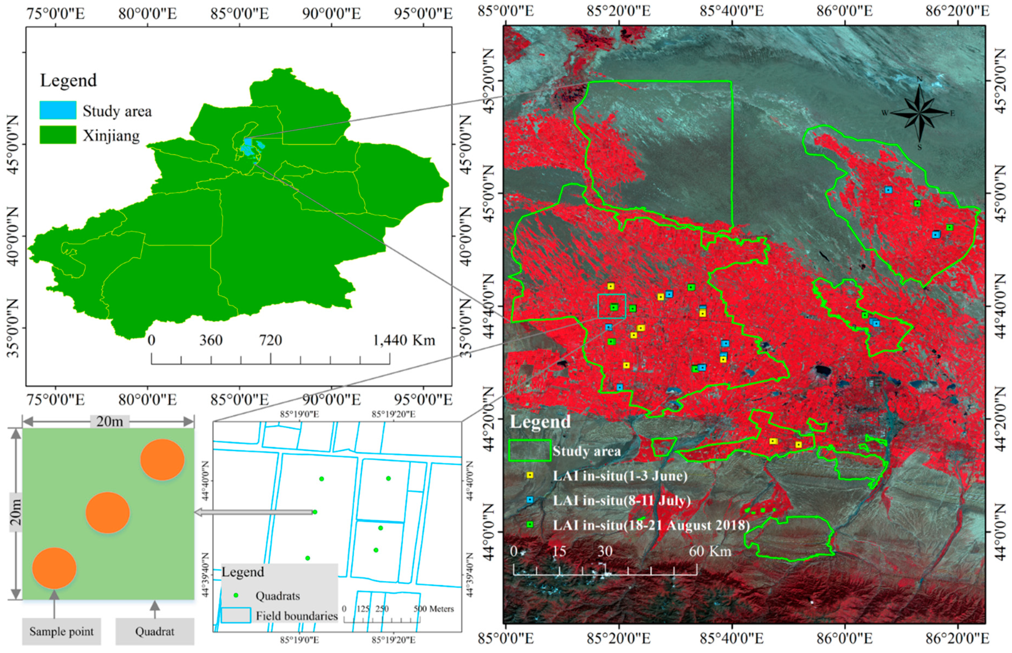
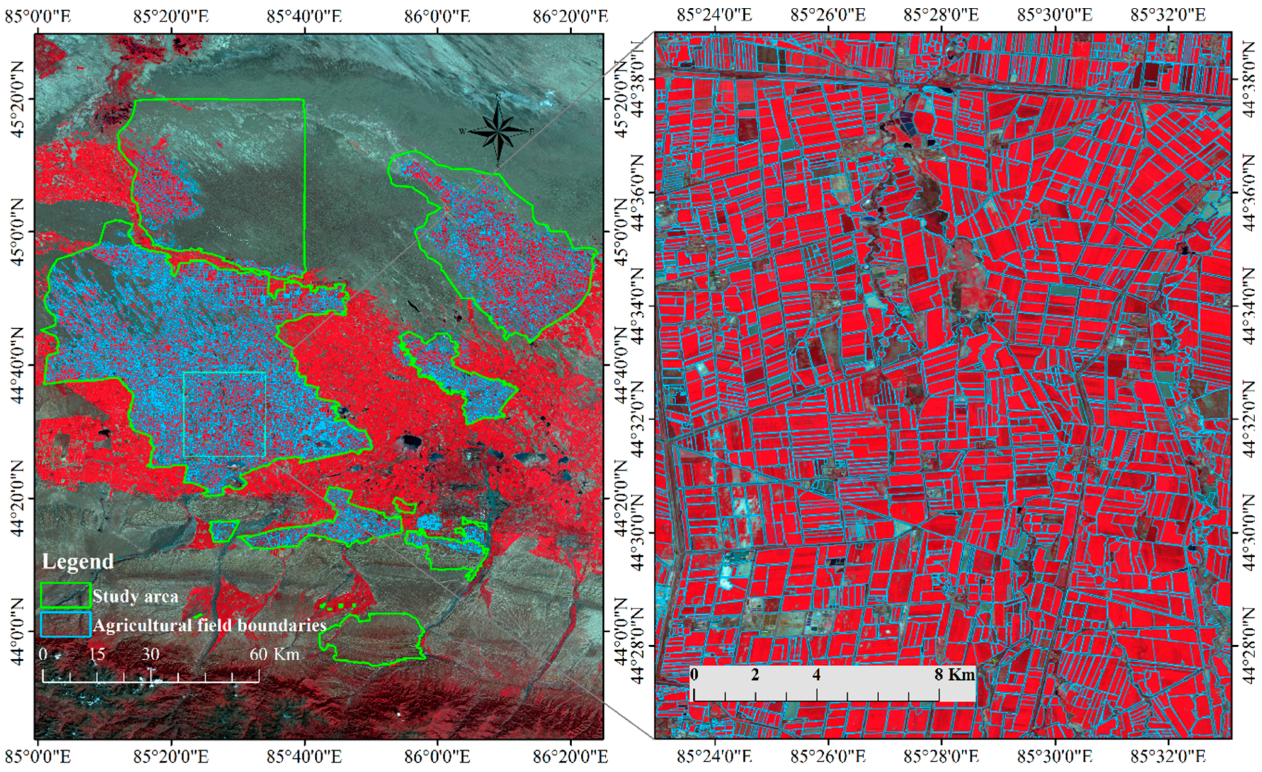
China is one of the largest cotton producers and importers in the world, and Xinjiang is the primary cotton-growing region in China [33,34]. The chosen study area was on a large agriculture region (6118.08 ) in Shihezi (44°37′ N, 85°42′ E), Xinjiang Province, China. The region is located in a temperate continental climate zone. The average field size in the study area is 73139.7 (18.07 acres), and the majority of fields have a flat topography, which is preferable for decametric remote sensing applications (e.g., Sentinel-2). The annual mean temperature of the study area is 7.39 °C, the annual total precipitation is 206 mm, and the average altitude is 450.8 m.
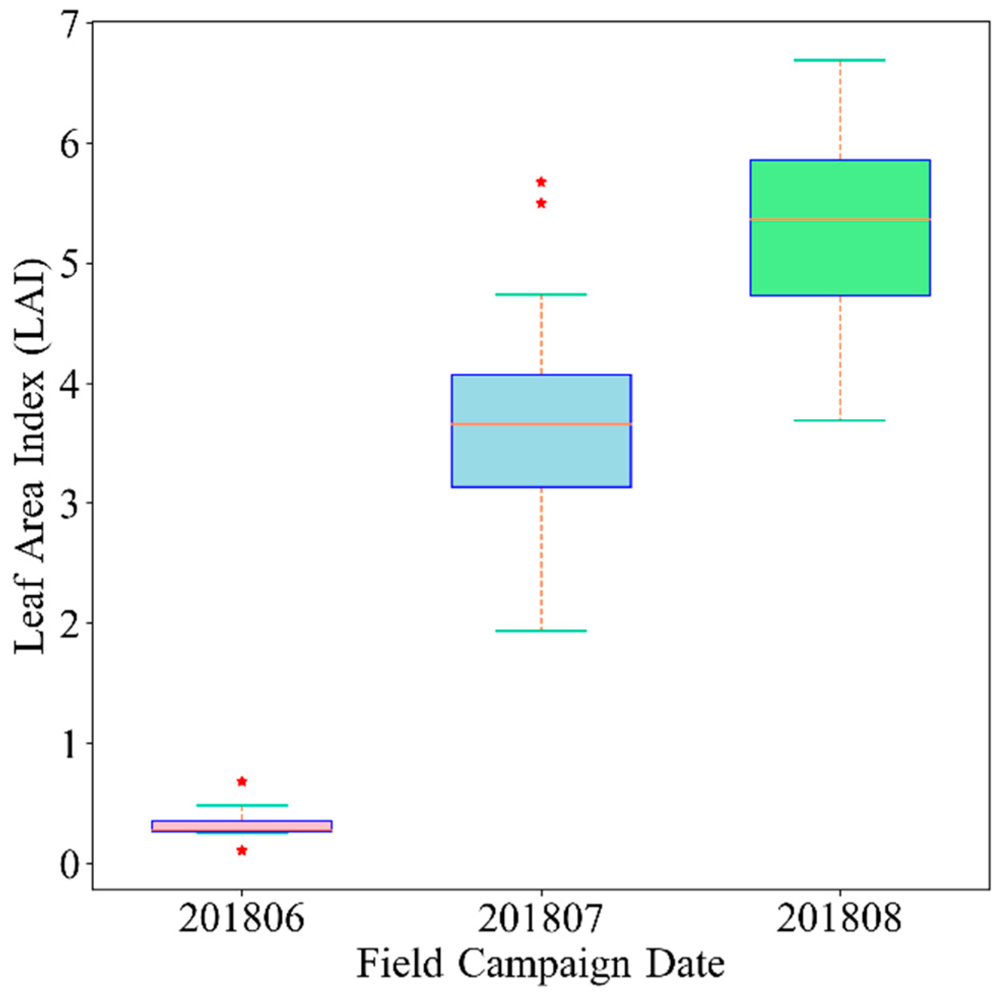
The field campaigns were conducted in early June 2018, mid-July 2018, and mid-August 2018 (Table 1), with 117 total quadrats obtained. Each quadrat was assigned one leaf area index (LAI) value, obtained as the average leaf area index (LAI) of the three sample points that matches the corresponding Sentinel-2 pixel (Table 2). Each sample point datum was collected using an LAI-2200C Plant Canopy Analyzer (Li-Cor, Inc., Lincoln, NE, USA). The main planted crops in the study area are cotton, grape, spring maize and winter wheat, and cotton holds the largest planting proportion, which is 71.7%. The cotton season is from mid-April to early October. The spring maize season is from mid-April to late September. The winter wheat season is from late September of the previous year to late June. Notably, the study area has completely achieved mechanization for agricultural production and management. Figure 1 shows the location of the study area and field observation sites with Sentinel-2A imagery (20 August 2018). A descriptive statistic of the measured cotton LAI at three observation dates is shown in Figure 2.
2.2. Sentinel-2 Data and Preprocessing
The remote sensing data used in this study were Sentinel-2 imagery. Sentinel-2 is a constellation of satellites, Sentinel-2A and Sentinel-2B, which were launched by the European Space Agency (ESA) on June 2015 and March 2017, respectively. Each satellite carries a MultiSpectral Instrument (MSI) that provides a variety of spectral bands covering the visible, near infrared and shortwave infrared bands. The MSI contains four bands at 10 m, six bands at 20 m and three bands at 60 m [36]. It is of great importance that the MSI incorporates three bands in the red-edge region, centered at 705, 740 and 783 nm, and two Shortwave Infrared (SWIR) bands centered at 1610 and 2190 nm at 20 m (S2-20 m). Many studies have revealed that the red-edge bands and SWIR bands have the potential to improve the accuracy of LAI retrievals [37,38,39], which open great opportunities for crop LAI retrievals considering Sentinel-2’s high revisit frequency. The Sentinel-2 spectral band characteristics are shown by Table 2.
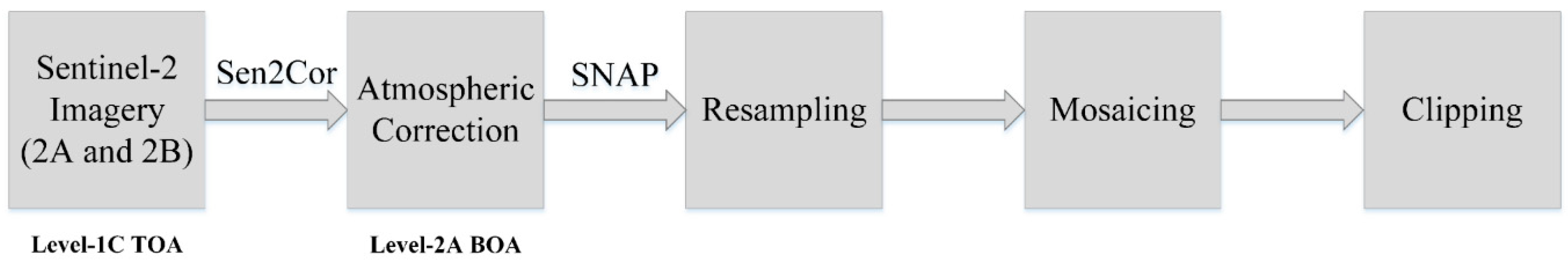
The acquired Sentinel-2 imagery products are Level-1C products, which are top of atmosphere (TOA) reflectances [40]. Atmospheric correction was conducted using the Sen2Cor (2.5.5, ESA, Frascati, Italy, 2018) and Sentinel Application Platform (SNAP) toolbox (6.0.1, ESA, Frascati, Italy, 2018) provided by the ESA to produce Level-2A bottom of atmosphere (BOA) products [41,42]. A flowchart of Sentinel-2 preprocessing is presented in Figure 3.
In this study, aiming at making full use of the spectral bands of Sentinel-2 (especially the red-edge and SWIR bands), we focus on S2-20 m (the same size as our quadrats) with 10 spectral bands considering the red-edge and SWIR spectral bands of Sentinel-2 imagery. A resampling process was performed using the Nearest Neighbor method with 4 spectral bands (B2, B3, B4 and B8) from 10 m to 20 m in the SNAP toolbox. Three of the atmospheric spectral bands at 60 m were not used in this study because these bands contributed to atmospheric applications, such as aerosol correction (B1), water vapor correction (B9) and cirrus detection (B10) [42]. The reflectance data collected on the Sentinel-2 images were using Extract by Points on the ArcToolbox of ArcGIS Desktop software (10.5, Environmental Systems Research Institute, Redlands, CA, USA, 2016), the points used to extract data on the Sentinel-2 images are the center GPS coordinate of the three sample points that represent one quadrat.
2.3. Global LAI Products
Many global LAI products with different spatial resolution and temporal characteristics has been produced, in which MODIS LAI products retrieved from Terra and Aqua platforms are one of the most famous global LAI products [2,43]. All MODIS products are available at [44]. In addition, GEOV1 LAI products have also been widely used for variety of applications. The GEOV LAI product was downloaded from the Copernicus Global Land Service [45]. More recently, new versions of these two products have been delivered with great improvement in spatial and temporal resolution [46,47,48]. Table 3 presents the main characteristics of the latest version of these two global LAI products.
3. Methods
ML algorithms can automatically learn the relationships in any given data between input (reflectances) and output (LAI). To identify the performance of five popular ML algorithms for cotton LAI retrieval, regression models were established based on artificial neural network (ANN), SVR, Gaussian process regression (GPR), random forest (RF) and gradient boosting regression tree (GBRT), at S2-20 m for the whole growth period of cotton (using all 117 quadrats data over the three observation dates).
All the ML models were implemented using the Scikit-learn package [49], which is an open-source Python [50] module project that integrates a wide range of prevalent ML algorithms [51]. All hyperparameter tuning of the models is based on GridSearchCV in the Scikit-learn package, which can evaluate all possible combinations of hyperparameter values using five-fold cross-validation to determine the best combination of hyperparameter values (the hyperparameter combination that has the best accuracy of the model in terms of root-mean-square error (RMSE)). Cross-validation are model validation techniques to obtain reliable and stable models. This study implemented a five-fold cross-validation, basically, the training datasets are split into five smaller sets, and a model is trained using four of the folds as training data, then the resulting model is validated on the remaining part of the data, the processes continues to circulate five times, and finally, the performance measure estimated by five-fold cross-validation is the average of the values computed in the loop. Training and testing sampling distribution has a great impact on machine learning regression algorithms (MLRAs), and some previous studies demonstrated that 70%/30% split option is appropriate for model training and validation [52,53,54], nonetheless, other studies argue that the 80%/20% split option is preferable [27,55]. In our study, to validate the performance of the ML models, all the datasets were randomly split into 75% (n = 87) for model training, and 25% (n = 30) for model validation. Regression models that achieve satisfactory performance in training datasets may fail to predict unseen datasets, and therefore, a model that performs well at both training and unseen testing datasets is referred to as having excellent generalization ability. This type of model could be used for crop LAI retrieval applications.
3.1. Artificial Neural Network (ANN)
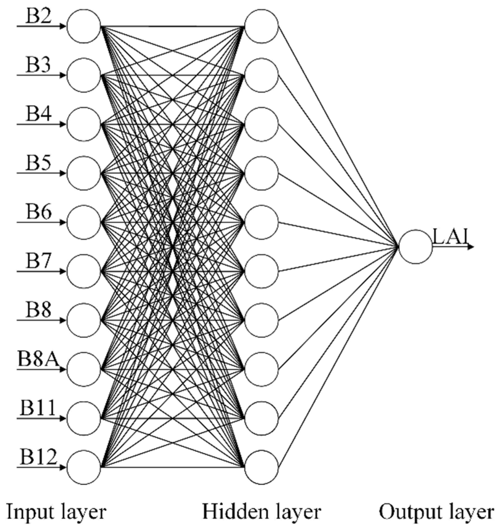
The ANN has been one of the most widely used ML algorithms for wide range of remote sensing applications. ANN is a computational model that is inspired by the human brain. ANN is formed by a collection of interconnected units (neurons) that learn from experience by modifying connections (weights) [56,57]. ANN usually consists of an input layer, hidden layer, and output layer. The backpropagation (BP) ANN used in this study implements a multilayer perceptron (MLP) algorithm that trains with a BP algorithm, while an MLP refers to a feedforward network that generalizes the standard perceptron by having a hidden layer that resides between the input and output layers. It has been demonstrated that MLP can approximate any continuous function to an arbitrary degree of accuracy, given a sufficiently large but finite number of hidden neurons [56,58]. In this study, the input layer and output layer are referred to as the Sentinel-2 spectral bands (reflectances) and the cotton LAI, respectively.
The major tuning hyperparameters for ANN are the number of hidden layers and the number of neurons in the hidden layer. Here, we used the one-hidden-layer network because it was demonstrated to be powerful enough to approximate any measurable function to any desired degree of accuracy [59]. Many studies have been dedicated to the investigation of the optimal number of neurons in the hidden layer, and several empirical equations have been proposed [60,61,62]. In this study, the number of neurons in the hidden layer is determined by the following equation [62]:
where is the number of neurons in the hidden layer, specifies the number of layers, and denotes the number of input neurons. The number of neurons in the hidden layer was set to ten in this study according to Equation (1). In the input layer, the input variables include 10 spectral bands. Other important hyperparameters were optimized using GridSearch and 5-fold cross-validation. The remainder of hyperparameters for the ANN model remain defaults. The structure of the neural network used in this study is presented in Figure 4. The hyperparameter values adopted in this study are listed in Table 4.
3.2. Support Vector Regression (SVR)
SVR is a significant application form of support vector machine (SVM), which was first introduced by Corinna Cortes (b. 1961 in Denmark) and Vapnik [63,64]. SVM is based on the idea of mapping the input space into a new feature space with higher dimensions using the kernel function, after which a hyperplane, known as the decision boundary, is constructed with the maximum margin [65,66]. SVM extension to SVR is realized by introducing an ε-insensitive region around the function, which is referred to as the -tube that best approximates the regression function [67]. Given training vectors , I = 1, and a vector , -SVR solves the following original problem:
where C > 0 is a regularization parameter that gives more weight to minimizing the flatness or error.
The principal hyperparameter of SVR is the kernel, as it defines the kernel functions of the model. The radial basis function (RBF) was selected as the kernel function because it has been found to be efficient and accurate for regression problems [68,69]. The RBF kernel is described as follows:
The SVR model is easy to establish because only two hyperparameters must be tuned: Penalty parameter C and the kernel coefficient gamma. The optimal values of the two hyperparameters that were optimized using GridSearch and 5-fold cross-validation are presented in Table 5. The remainder of hyperparameters for the SVR model remain defaults.
3.3. Gaussian Processes Regression (GPR)
A Gaussian process is a stochastic process that is formed by a collection of random variables and has a Gaussian probability distribution [70]. The major factor in the Gaussian process is the covariance function known as the kernel function. The learning problem in the Gaussian process amounts to adjusting the covariance hyperparameters. The mean function and covariance function characterize the Gaussian process , which can be described as follows:
For simplicity, we usually consider the mean function to be zero.
Similar to SVR, GPR has been advanced to solve complex nonlinear problems through projection of inputs into high dimensional space by applying highly flexible kernels, where such a technique is referred to as kernel trick. Additionally, GPR models have a great ability to provide the most informative feature (spectral band) from the input dataset. In this study, we used the sum of an RBF and a noise component function kernel:
where is the scaling factor, is the length-scale, and corresponds to the independent noise component.
Beyond the kernel functions, alpha and n_restarts_optimizer, are significant for the GPR model. The results of hyperparameter tuning using GridSearch and 5-fold cross-validation are shown in Table 6 as follows. The remainder of hyperparameters for the GPR model are set as defaults.
3.4. Random Forest (RF)
RF has been a prevalent ML algorithm for a wide range of fields for classification, regression and other complicated problems. As one of the ensemble learning methods, RF grows a multitude of decision trees as base learners, and combines these trees together to obtain a better performance by averaging the predictions [71,72]. Each tree grows independently with training samples obtained using bootstrap sampling from the original data. Then, m variables out of M input variables are chosen, after which the best of m is used for splitting the node (note that m M). The final prediction comes from the averaging predictions of each independent tree. This kind of technique is referred to as bagging. RF models can provide feature importance estimates, which enables insight into feature selection processes.
Key hyperparameters include n_estimators, max_depth, min_samples_split and min_samples_leaf. Hyperparameter tuning results using GridSearch and 5-fold cross-validation are displayed in Table 7. The remainder of the RF model hyperparameters are set as defaults.
3.5. Gradient Boosting Regression Tree (GBRT)
GBRT, also known as gradient boosting decision tree (GBDT) or multiple additive regression tree (MART), is one of the most widely used ML algorithms for the model’s great generalization ability and highly robust performance in practical applications, and this GBRT was introduced by Friedman [73,74]. As one of the ensemble learning methods that combines different weak learners to generate strong learners, GBRT uses boosting techniques that aim to reduce bias, rather than bagging (e.g., RF algorithm), which aims to reduce variance. To evaluate the accuracy of the model, a variety of loss functions can be used during boosting, including least squares, least absolute deviation, Huber and quantile for regression, binomial deviance, multinomial deviance, and exponential loss for classification. GBRT considers additive models of the following form:
where represents the basis learners in boosting. Then, GBRT builds the additive model in a forward stagewise fashion:
At each stage, the decision tree is chosen to minimize the loss function , given the current model and its fitting of :
The initial model is problem specific. Gradient boosting attempts to solve this minimization problem numerically via the steepest descent. The steepest descent direction is the negative gradient of the loss function evaluated at the current model , which can be calculated for any differentiable loss function as follows:
where the step length is chosen using a line search:
The GBRT algorithm can provide feature relevance information and partial dependence, where this partial dependence shows the dependence among the target response and the most important features (not shown in this study). However, despite the GBRT’s demonstrated satisfactory accuracy for versatile domains of regression problems [29,75,76], to our knowledge, this algorithm has not been previously applied to crop LAI retrievals with remote sensing. GBRT should be studied as it might be a promising alternative in crop LAI retrieval with remote sensing.
With regard to GBRT model hyperparameters, loss, n_estimators, max_depth, min_samples_split and min_samples_leaf are selected for hyperparameter tuning using GridSearch and 5-fold cross-validation, the results are exhibited in Table 8. The remainder of the GBRT model hyperparameters are set as defaults.
3.6. Performance Evaluation
To evaluate the performance of the ML regression models, the root mean square error (RMSE), mean absolute error (MAE) and coefficient of determination () between the measured and predicted values were used to assess the performance of the models. The RMSE, MAE and are calculated as follows:
where , is the estimated cotton LAI value, is the measured cotton LAI value and is the number of validation datasets. The higher the , the smaller the RMSE and MAE, and thus the higher the model precision and accuracy.
4. Results
4.1. Performance Evaluation
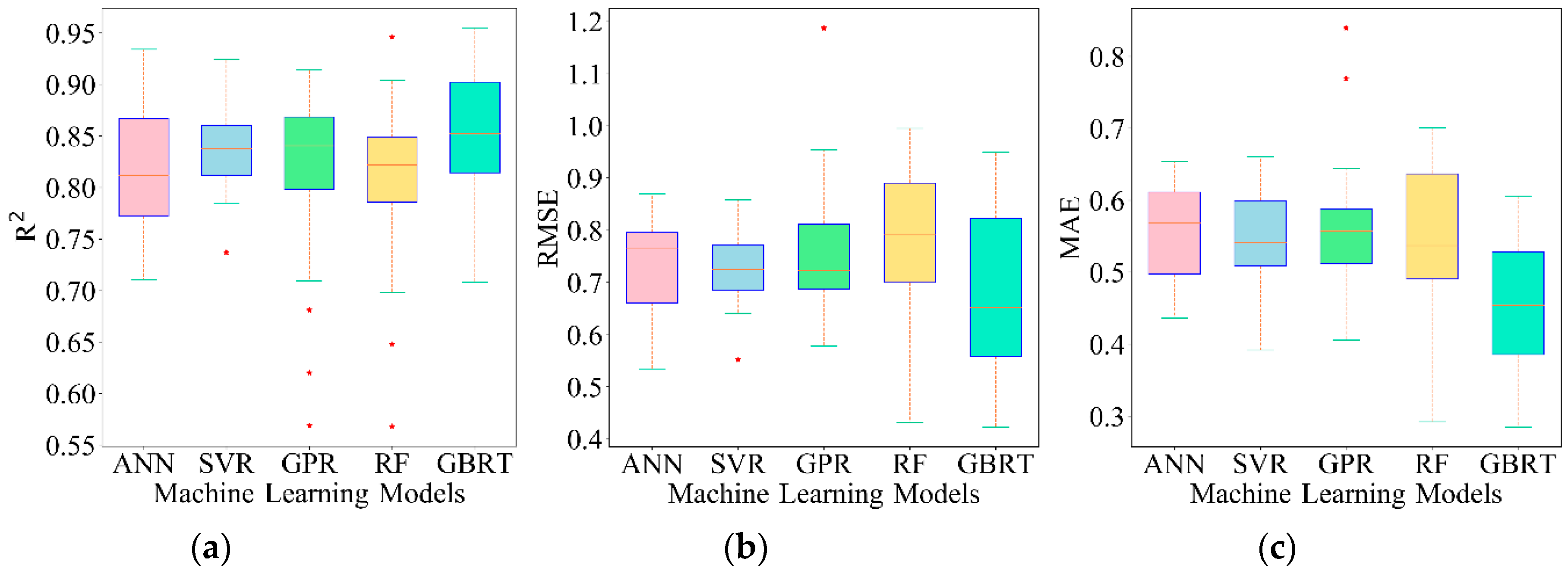
To avoid skew results caused by the random sampling of training and testing datasets, we performed 20 random repetitions of the five ML regression models (87 samples for training and 30 for testing). The performance of five ML models with respect to , RMSE and MAE is displayed in Figure 5. GBRT surpasses the other models on the average ( = 0.854, = 0.674 and = 0.456), however, GBRT acts less robust to the training/testing random split according to the distribution of , RMSE and MAE. RF delivers the worst accuracy on the average ( = 0.807, = 0.781 and = 0.545), and it also acts less robust to the training/testing random split. Nonetheless, SVR achieves a desirable result while it also acts reasonably robust to the training/testing random split ( = 0.835, = 0.730 and = 0.550), which indicates that SVR is highly stable to the random sampling processes. Overall, all models achieved satisfactory performances, which indicates that ML algorithms are appealing methods for cotton LAI estimation.
4.2. Computational Efficiency
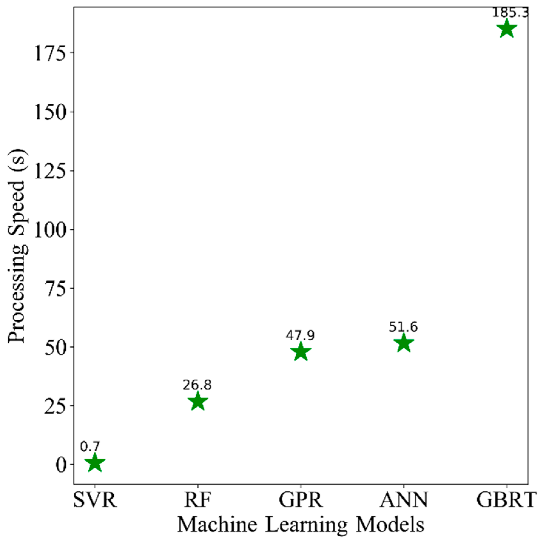
Beyond the model accuracy of the five models for the training and testing random split, it is of particular relevance to compare the computational efficiency (time required to the model during training and validation processes) of the models, as it is an important criterion for operational algorithms. All models were implemented in a Python environment on an Intel(R) Xeon(R) CPU E5-2620 v2 @ 2.10 GHz processor and installed memory (RAM) of 32.0 GB. The computational efficiency is recorded from the 20 repetitions in Section 4.1. The averaged results of 20 repetitions are illustrated in Figure 6. Large differences among the five ML models are clearly found. SVR performs incredibly fast (less than 1 s). However, GBRT is frustrating, owing to the large amounts of its hyperparameter tuning processes. In general, SVR is able to deliver near real time operational products with a highly efficient processing speed, whereas the GBRT model is not recommended for this kind of application, because the GBRT model is computationally more demanding. RF, GPR and ANN showed moderate performances in terms of computational efficiency.
4.3. Sensitivity to Training Sample Size
We use , RMSE and MAE between the predicted LAI values and measured LAI values to assess the sensitivity of five ML methods to the training sample size. Eight datasets with different sample sizes (17-87) were generated by randomly sampling from the total training datasets (87 samples) at intervals of 10. Table 9 shows the number of training and testing samples of the eight datasets, while the testing datasets keep as the same datasets with 30 samples.
To evaluate the robustness of five ML models for the training samples, we conducted 10 random repetitions of each model and provided the corresponding standard error. The standard error is given as follows:
where denotes the standard deviation, represents the number of repetitions.
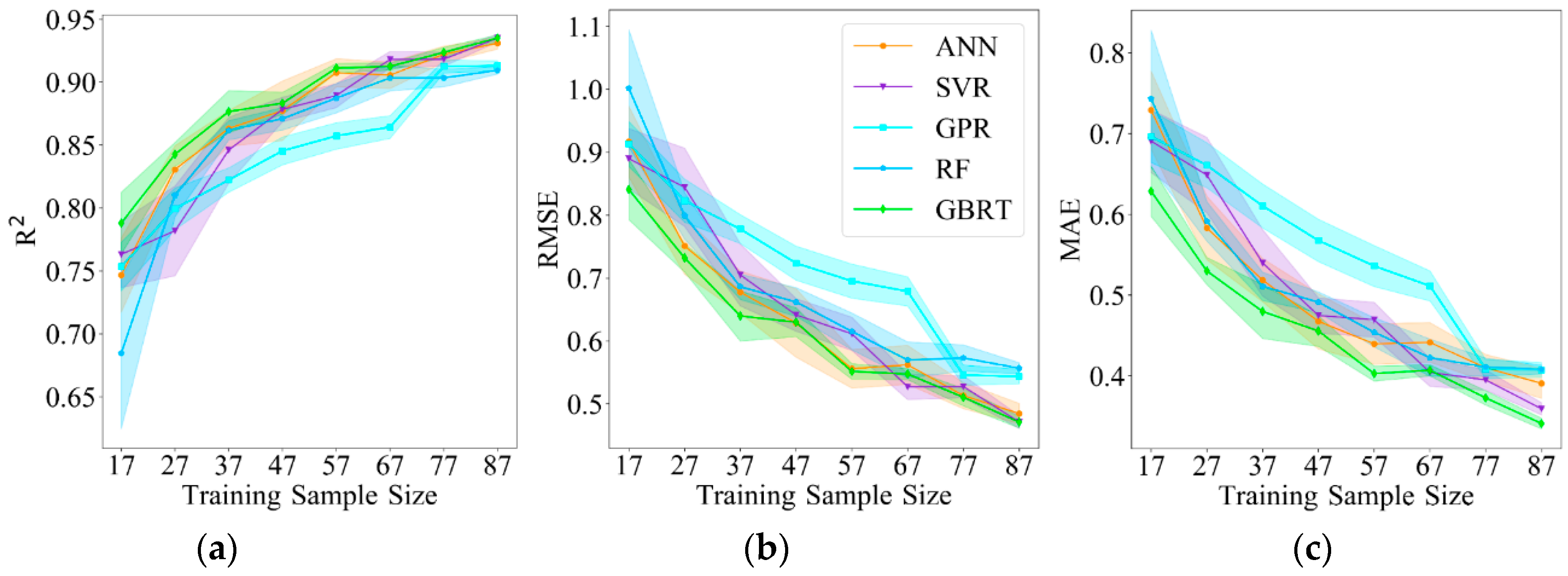
Figure 7 shows the changes in , RMSE and MAE as the training sample sizes varied, the standard error is given at each training sample size (filling area of each model), lower values of the filling area corresponds to smaller standard error, and consequently, more robust model performance. According to Figure 7, different sensitivity performances of the sample size variation are found among the ML models. GPR and GBRT show robust performances for the training samples according to the standard error of different models. GBRT produces a remarkable performance for the training samples that is more robust than the other models, GPR behaves suboptimally. ANN and SVR are very sensitive to the training samples. Moreover, all models behave more robust with the growth of training sample size according to the variation of standard error. In summary, the model accuracy improves overall with an increasing training sample size, while GBRT provides the most robust performance for the training samples, and the best model accuracy among the variations in training sample size on average ( = 0.884, = 0.615 and = 0.452, calculated by all the 8 groups of training sample size).
4.4. Sensitivity to Spectral Bands
Variable and feature selection have been one of the most significant processes in ML, with the aim of improving model accuracy and accelerating model processing. With 10 spectral bands of Sentinel-2 available (B2, B3, B4, B5, B6, B7, B8, B8A, B11, B12), it may not be practical to evaluate the performance of all the possible band combinations. This process could be challenging, as the characteristics of different ML models are distinct, and thus it is challenging to conduct a comparison among the different models under a unified standard. For example, GPR, RF and GBRT could provide feature relevance (spectral bands relevance) information that enables insight into feature selection processes, however, the feature relevance results are subject to the model itself, in other words, we could obtain different feature selection schemes, and such information is practical with single ML model based applications. In addition, ANN and SVR are not able to deliver feature relevance information.
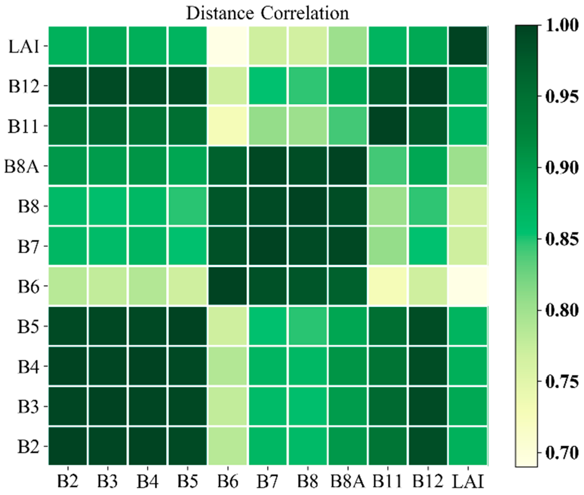
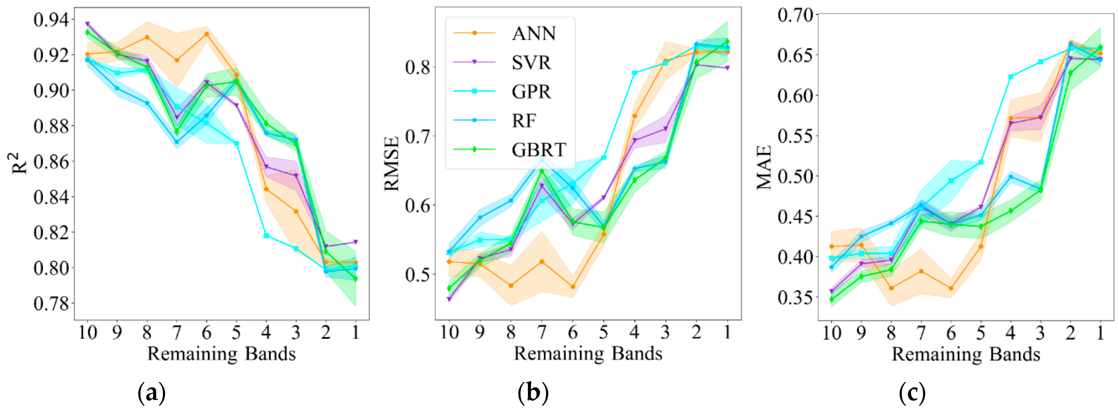
Székely, Rizzo, and Bakirov [77] proposed the distance correlation (dCor) to measure the dependence of random vectors. dCor ranges between 0 and 1, and dCor (X, Y) = 0 only if X and Y are independent, which is effective in the feature selection processes [78,79,80]. To identify the optimal number of Sentinel-2 spectral bands required for cotton LAI retrieval using MLRAs, we used the distance correlation combined with the backward elimination method [81,82]. We also performed 10 random repetitions of each model to assess the model’s robustness with the spectral bands. Notably, the distance correlation is subject to the training dataset adopted in this study. Figure 8 displays the distance correlation among the 10 spectral bands and LAI. The ranking of the dCor values between the 10 spectral bands and LAI are identified as B12 > B3 > B4 > B2 > B5 > B11 > B8A > B7 > B8 > B6 (B12: 0.88631, B3: 0.88630, B4: 0.88016, B2: 0.87721, B5: 0.87400, B11: 0.87338, B8A: 0.80219, B7: 0.76812, B8: 0.76585, B6: 0.68998). The visible and SWIR bands occupied the top rankings, while differences among the red-edge bands were distinct. The sensitivity results of different ML models to spectral bands using dCor and the backward elimination method (iteratively removing the spectral band with the lowest dCor value until only one spectral band is left) are shown in Figure 9, similarly, the standard error is given at each spectral bands combination (filling area of each model), lower values of the filling area corresponds to smaller standard error, and consequently, more robust model performance. Differences exist among the sensitivity of the models with the reduction in spectral bands. A turning point occurred at 6 for ANN, the accuracy begins to increase with the reduction in spectral bands before 6, though with some fluctuations, and then, the accuracy begins to decrease dramatically until reaching approximately 3. Similar trends are found among all the models except for GPR, as there is a relatively strong fluctuation at 7. GPR has a stable performance after 4. SVR, GPR and RF are robust for the spectral bands according to the standard error. Overall, model accuracy decreases as the spectral bands decrease, although there are some fluctuations in the models, whereas ANN provides the best model accuracy among the spectral band reductions on average ( = 0.881, = 0.625 and = 0.480, calculated by all the 10 groups of spectral bands).
The minimum number of bands required for cotton LAI retrieval are recognized as 6 for ANN and SVR, 5 for RF and GBRT, and 8 for GPR, in other words, increasing of the spectral bands of Sentinel-2 does not significantly improves the model accuracy. Given the recognized number of spectral bands of each of the ML models, this is vital for associated applications with great amounts of samples, as it may reduce model processing time and desirable model accuracy could be acquired in the meantime.
4.5. Comprehensive Evaluation
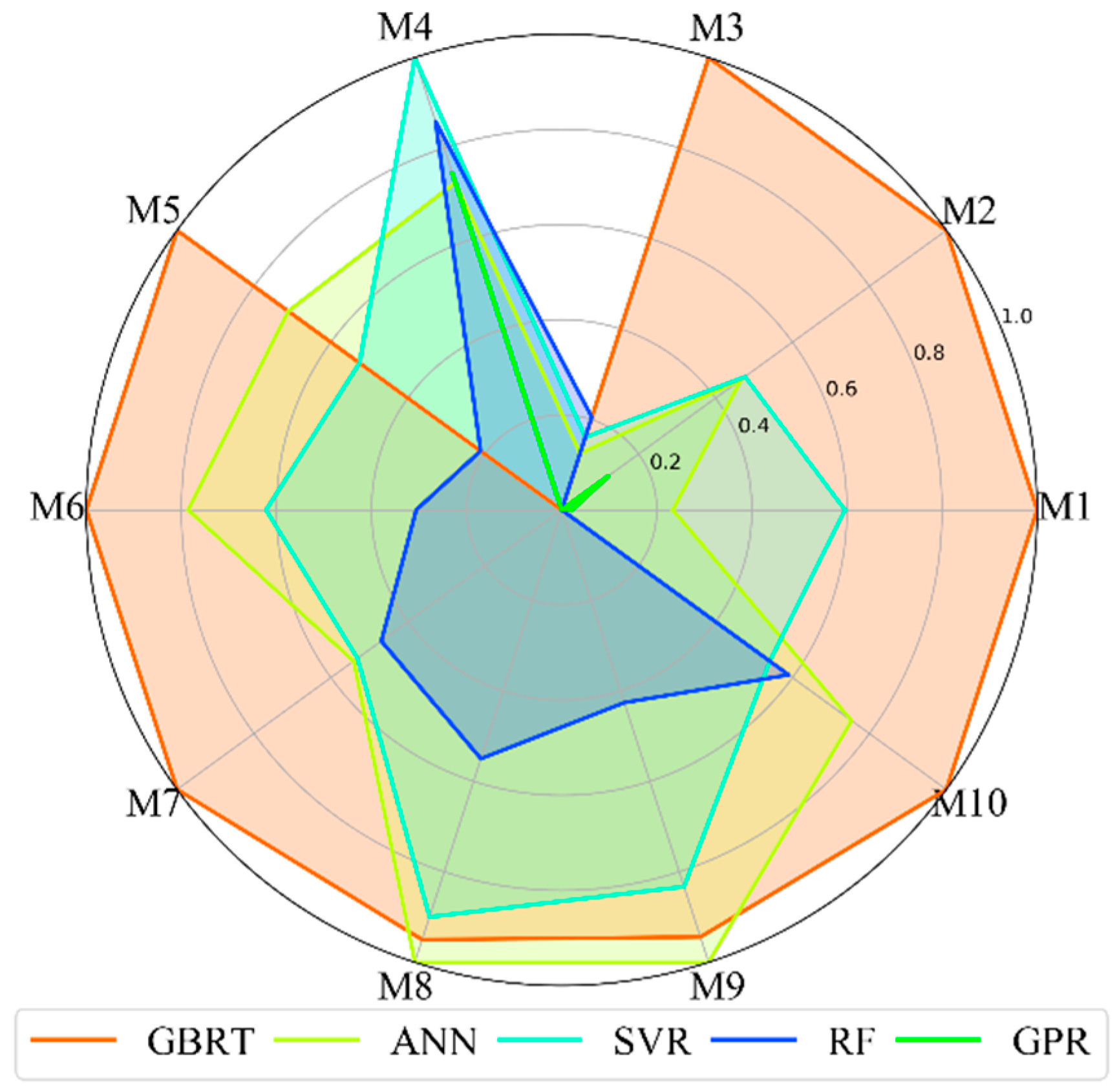
In this study, we conducted a comparison of five universal MLRAs for cotton LAI retrieval with regard to model accuracy, computational efficiency, sensitivity to training sample size and sensitivity to spectral bands. In this section, we provide a comprehensive evaluation of five ML algorithms according to the obtained results, which were discussed earlier in this paper. To combine all the metrics, we performed a standardization process on the results. The mean values of the results in the sensitivity analysis (training sample size and spectral bands) were used, and we make RMSE, MAE and processing speed negative for the sake of comprehensive comparison. An alternative standardization is interval scaling, which is as follows:
where denotes the maximum value of the data, and represents the minimum value of the data. The results are displayed in Figure 10, and the metrics used in the radar chart and its corresponding implications are displayed in Table 10. Clearly, GBRT shows an outstanding performance from a comprehensive viewpoint, however, GPR shows the worst performance. ANN and SVR show moderate performances.
4.6. Final LAI Maps
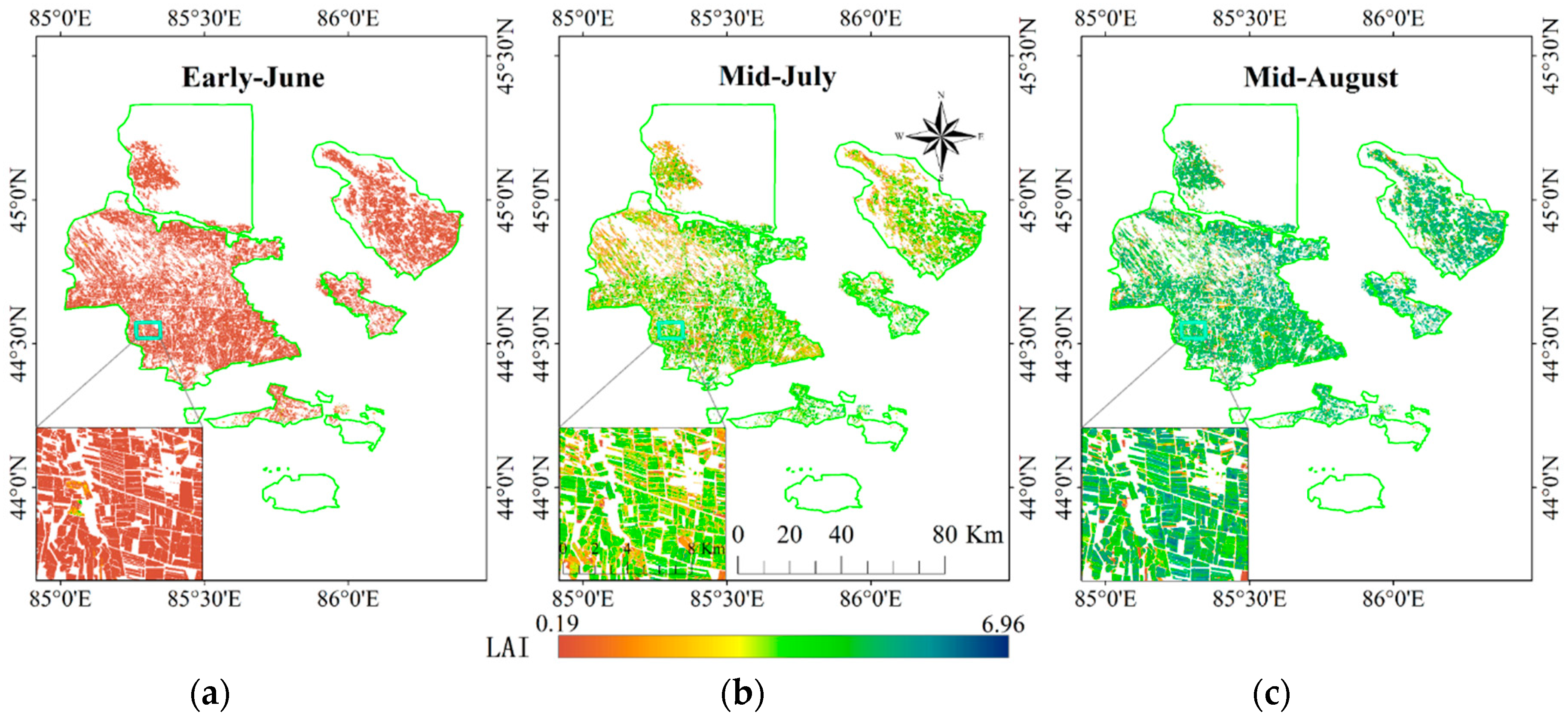
The best performing ML regression model has been applied to map cotton LAI with Sentinel-2 imagery, as analyzed in previous sections, we use the GBRT model to map cotton LAI in the study area. The fields in the study area are regular, we conducted a manual vectorization based on Google Earth image data to obtain accurate agricultural fields boundaries, and Landsat 8 image data were collected to update the fields, as Google Earth image data has poor temporal information. Totally, 40,211 fields were collected by this way in the study area. Figure 11 displayed the agricultural fields boundaries. A per-field crop classification was performed to extract cotton fields. The final cotton LAI map was obtained by masking the results using the extracted cotton fields. Figure 12 presents the final cotton LAI map. From Figure 12, it is clear to find that there is an increasing trend of cotton LAI growth, as revealed by Figure 2.
In the early June cotton LAI map, some areas have LAI values much larger than the whole map (green color), as well as LAI values much smaller found in mid-July and mid-August (orange color), these fields are some other crops rather than cotton, and it can be ascribed to the misclassification.
4.7. Comparison with Global LAI Products
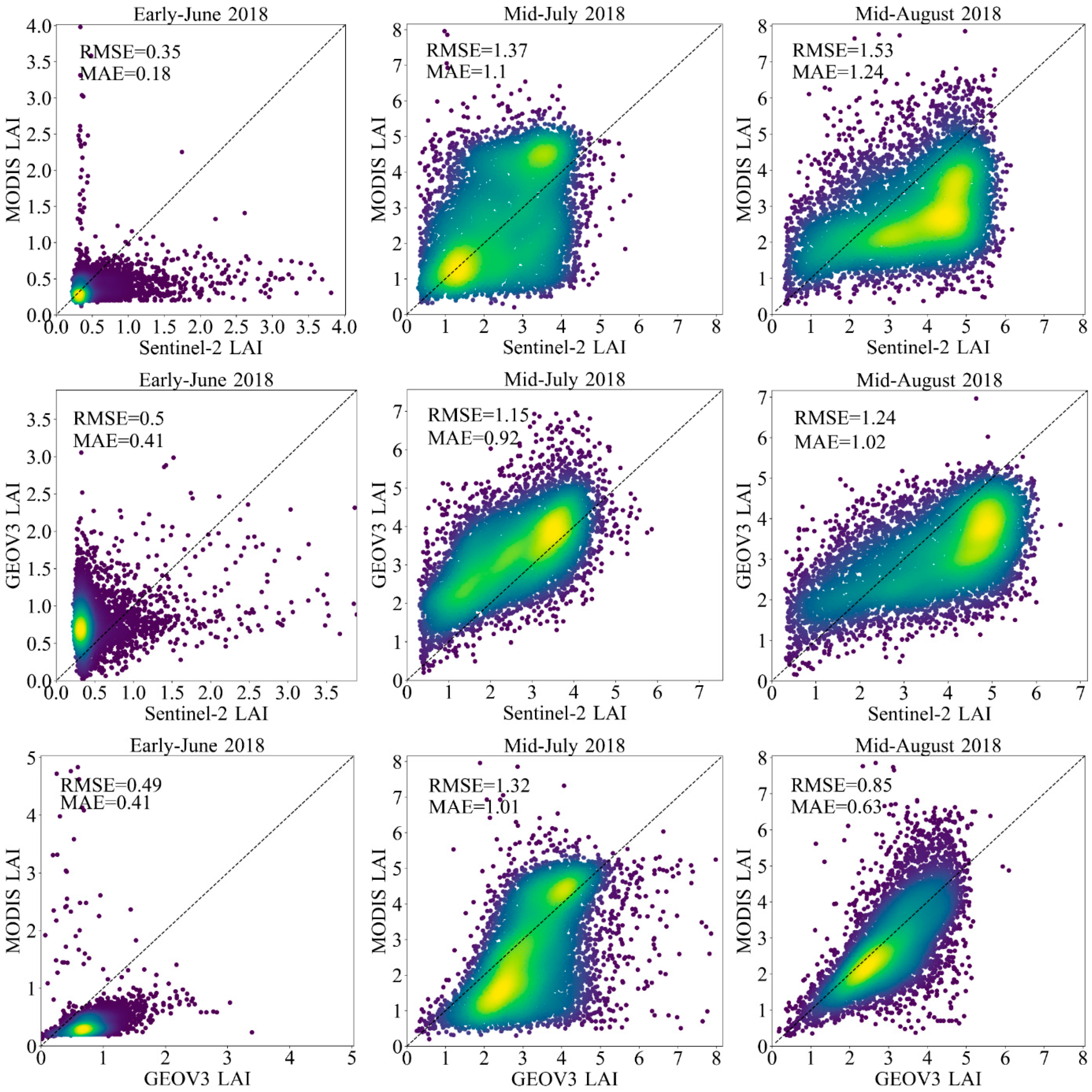
The validation of moderate-resolution products are key steps to assess the quality of the global LAI products. In this study, we performed a comparison among GEOV3, MODIS LAI products and upscaled Sentinel-2 LAI to assess the quality of these two products in Northwest China. To conduct the comparison of the cotton LAI results obtained using the GBRT model with global LAI products, we choose the closest dates of the products at a spatial resolution of the products to minimize the spatial and temporal differences [2].
All Sentinel-2 LAI maps were resampled to the same spatial resolution of MODIS and GEOV3 LAI products, and then GEOV3 LAI product were also resampled to the same spatial resolution of MODIS LAI product to make a straight comparison of these two products. Figure 13 shows the scatter plots among the comparison of GEOV3, MODIS and Sentinel-2 cotton LAI over three observation dates. Regarding the comparison of the MODIS LAI product and Sentinel-2 LAI maps, it was found that both the MODIS LAI product and the Sentinel-2 LAI suffered from the influence of the background, and are kind of overestimated in some areas in early June 2018. MODIS LAI product underestimated a little bit in mid-August 2018. In terms of GEOV3 LAI product and Sentinel-2 LAI maps, the GEOV3 LAI product overestimated at some areas both in early June and mid-July 2018, and underestimated in mid-August 2018. Finally, with respect to the comparison of the two global LAI products, relatively, large differences are found in early June and mid-July 2018, whereas a good relationship appeared in mid-August 2018.
5. Discussion
Over the last decade, there has been a considerable increase in the introduction of ML algorithms to remote sensing for a wide range of fields. Crop biophysical parameters (e.g., LAI) are key variables for a wide range of applications. With the progress of remote sensing techniques, we are able to acquire high dimensional (spatial, temporal, and spectral) remote sensing data, which demands more efficient, accurate and robust algorithms in a wide variety of applications with remote sensing. In this context, there is great potential for ML algorithms to be used in a wide range of remote sensing applications.
The diversity of available ML algorithms poses great challenges for the selection of MLRAs, as well as the decision of optimal number of training sample size and spectral bands to different MLRAs. Besides, another significant problem that may arise involves hyperparameter tuning in the application of ML algorithms. In general, experience is required to obtain satisfactory results for ML algorithms, and experiments with a large number of datasets may be needed, which are generally not available. Accordingly, it is necessary to perform a comparison of different fashionable ML models to support better remote sensing applications. In this study, we focus on the comparison of five well-known ML algorithms for cotton LAI retrievals with Sentinel-2 imagery, because these algorithms have a wide range of applications in remote sensing. Additionally, the hyperparameter tuning results of five prominent ML models are provided. Our study could provide support for associated remote sensing studies based on ML algorithms.
Furthermore, a comparatively great fluctuation is observed at 7 among all the models except for GPR in Figure 9, the previous removing spectral band is the red-edge band (B7), which indicates that having low dCor values do not necessarily correspond to being less important for LAI retrieval. Notably, ensemble methods (RF and GBRT) and GPR models have a great benefit of delivering feature importance information (not shown in our study), which provides insight into the greatest contributing features of the model. Such information could be used for better model interpretation, and this information is also useful for feature selection processes when applied to models that contain a great number of features.
In related studies, Verrelst, et al. [55] compared four ML algorithms (NN, SVR, KRR and GPR) using simulated Sentinel-2 and 3 data to assess three biophysical parameters (Chlorophyll content, LAI and FVC). GPR outperformed the other regression methods for the majority of Sentinel configurations, whereas in our study, GPR performed worse than the other regression methods. Results that differ from our study may be for the following reasons. First, we used real Sentinel-2 data rather than simulation data, and it may be difficult to represent the performance of real Sentinel-2 data with simulation data. Second, we focus on cotton crops over the entire growth period rather than on various crop types. In addition, there may be different hyperparameter settings between models. Finally, there are differences between the Sentinel-2 bands, and we used 10 spectral bands (SWIR included). Yuan, et al. [83] compared the RF, ANN and SVM regression models for soybean LAI retrieval using unmanned aerial vehicle (UAV) hyperspectral data with different sampling methods. The results showed that RF is suitable for the whole growth period of soybean LAI estimation, while ANN is appropriate for a single growth period. Siegmann and Jarmer [84] compared SVR and RFR for wheat LAI estimation using hyperspectral data, and the results showed that SVR provided the best performance of the entire dataset. Different from previous studies, we considered the GBRT model due to its highly robust performance over a wide range of applications. We further explored the sensitivity of different ML algorithms to training sample size and Sentinel-2 spectral bands. The results show that GBRT achieves the best performance, and GBRT was more robust for the training samples than the other models.
Despite the promising results revealed by five ML regression methods, there are some limitations of our study, and further studies are needed to assess the generalization ability of the five ML regression methods. Firstly, we focus on only one crop type, and the performance of ML regression methods for other crop types has not been validated. It is necessary to evaluate ML algorithms with various crop types, provided there are enough field measurement LAI data of different crop types available.
Secondly, some other crop biophysical parameters (e.g., Chlorophyll content and FVC) demand evaluation as well as ML regression methods, as different results may appear with different ML algorithms and different crop biophysical parameters. Thirdly, there are limitations with Sentinel-2 spectral bands sensitivity analysis, since some spectral bands are highly correlated, and redundancies remain among the spectral bands, so this process would be worth further investigations to explore a better spectral bands sensitivity analysis. Additionally, there are limitations to our quadrats in the field campaigns, as we chose only three sample points to represent a quadrat (20 m 20 m). Finally, the performance of five MLRAs has not yet been evaluated for large amounts of data (e.g., tens of thousands of data) due to the limited number of samples in our study, however, it remains to be seen whether a favorable performance can be obtained. In consideration of the ability of ML techniques, it is expected to obtain a better accuracy of the regression models provided there are enough samples, and a turning point should be obtained, as has been demonstrated in previous studies [19]. While before the turning point, the model accuracy increased rapidly with the increase in the training sample size, whereas, after the turning ponits, the model behaves more stable, in other words, the model accuracy remmained unchanged with the increasing of training sample szie. Future studies are required to investigate this problem.
With the advance in ML technology, deep learning, a new subfield of ML, has been applied successfully to many remote sensing domains, especially with a large quantity of data [85]. It is not necessary to construct complex ML models (deep learning-based models) in our study, as traditional ML algorithms have the capability of establishing efficient, accurate and robust estimation models for cotton LAI retrieval. However, as there are greater amounts of data available, deep learning techniques may be promising alternatives for handling such large volume datasets and complex relationships among the input datasets, which deserve further study.
6. Conclusions
With the challenges of selecting ML algorithms for crop LAI estimation, the results of this study have great implications for the selection of appropriate ML models from the diversity of available ML algorithms, and at the same time, these same results provide the optimal number of training sample size and spectral bands of Sentinel-2 for each model required for cotton LAI retrieval. Regarding the comparison of different ML models for cotton LAI retrieval employed in our study, the GBRT model outperforms the other ML models according to our results. Our findings increase the potential for cotton LAI retrieval with Sentinel-2 imagery, and may be transferrable to other associated problems related to agricultural remote sensing applications. On the other hand, the GBRT model is computationally demanding, which may be a significant problem with a large scale of data. However, GBRT can challenge the model accuracy and computational efficiency selection problems. Considering the computational efficiency, SVR exhibits considerable computational superiority over the other ML models.
Regarding the sample size sensitivity of ML models, model accuracy increases with the growth of the training sample size, and the GBRT produces the most robust performance for the training samples with respect to the standard error and the best model accuracy on average.
In terms of spectral band sensitivity analysis, the distance correlation results showed that the SWIR and visible bands have great potential to improve the accuracy of cotton LAI retrievals. By using dCor combined with the backward elimination method, the model accuracy decreases with the reduction in spectral bands. SVR, GPR and RF perform robustly with the spectral bands, and ANN provides the best accuracy on average. The minimum number of bands required for cotton LAI retrieval are recognized as 6 (ANN), 6 (SVR), 5 (RF), 5 (GBRT) and 8 for GPR.
A comprehensive evaluation has been employed to identify the performance of five ML models, considering a combination of model accuracy, computational efficiency, sensitivity to training sample size and sensitivity to spectral bands. The comprehensive performance of the models is identified as GBRT > ANN > SVR > RF > GPR.
Despite the different performances of the five ML regression models, MLRAs are promising ways to retrieve cotton LAI with Sentinel-2 imagery because the MLRAs all achieved encouraging accuracies. With profound applications for a diversity of ML algorithms in remote sensing, MLRAs may provide positive effects for remote sensing applications in terms of classification, regression, and other associated problems.
Author Contributions
Conceptualization, J.M. and H.M.; Methodology, H.M.; Formal Analysis, H.M.; Investigation, H.M., F.J., Q.Z. and H.F.; Data curation, H.M.; Writing—Original Draft Preparation, H.M.; Writing—Review and Editing, J.M.; Visualization, H.M.
Funding
This research was funded by GF6 Project under grant No. 30-Y20A03-9003-17/18 and 09-Y20A05-9001-17/18; the National Natural Science Foundation of China (41871261); and the open fund of the Key Laboratory of Oasis Eco-agriculture, Xinjiang Production and Construction Group (201701).
Acknowledgments
We are grateful to Agricultural College of Shihezi University for providing help in field campaigns. We would like to acknowledge the authors who contributed to the development of Scikit-learn project. We acknowledge the Copernicus Global Land Service, and the Land Processes Distributed Active Archive Center (LP DAAC) within the NASA Earth Observing System Data and Information System (EOSDIS) for providing the global LAI products. We are thankful to the three anonymous reviewers for their insightful comments and suggestions helped to clarify and improve the manuscript.
Conflicts of Interest
The authors declare no conflict of interest.
References
- Chen, J.M.; Black, T.A. Defining leaf-area index for non-flat leaves. Plant Cell Environ. 1992, 15, 421–429. [Google Scholar] [CrossRef]
- Garrigues, S.; Lacaze, R.; Baret, F.; Morisette, J.T.; Weiss, M.; Nickeson, J.E.; Fernandes, R.; Plummer, S.; Shabanov, N.V.; Myneni, R.B.; et al. Validation and intercomparison of global Leaf Area Index products derived from remote sensing data. J. Geophys. Res.-Biogeosci. 2008, 113. [Google Scholar] [CrossRef] [Green Version]
- Asner, G.P.; Scurlock, J.M.O.; Hicke, J.A. Global synthesis of leaf area index observations: Implications for ecological and remote sensing studies. Glob. Ecol. Biogeogr. 2003, 12, 191–205. [Google Scholar] [CrossRef]
- Buermann, W.; Dong, J.R.; Zeng, X.B.; Myneni, R.B.; Dickinson, R.E. Evaluation of the utility of satellite-based vegetation leaf area index data for climate simulations. J. Clim. 2001, 14, 3536–3550. [Google Scholar] [CrossRef]
- Yuan, H.; Dai, Y.J.; Xiao, Z.Q.; Ji, D.Y.; Shangguan, W. Reprocessing the MODIS Leaf Area Index products for land surface and climate modelling. Remote Sens. Environ. 2011, 115, 1171–1187. [Google Scholar] [CrossRef]
- Van den Hurk, B.; Viterbo, P.; Los, S.O. Impact of leaf area index seasonality on the annual land surface evaporation in a global circulation model. J. Geophys. Res.-Atmos. 2003, 108, 4191. [Google Scholar] [CrossRef]
- Cheng, Z.Q.; Meng, J.H.; Wang, Y.M. Improving spring maize yield estimation at field scale by assimilating time-series HJ-1 CCD data into the WOFOST model using a new method with fast algorithms. Remote Sens. 2016, 8, 303. [Google Scholar] [CrossRef]
- Systematic Observation Requirements for Satellite-Based Products for Climate 2011 Update: Supplemental Details to the Satellite-Based Component of the “Implementation Plan for the Global Observing System for Climate in Support of the UNFCCC (2010 Update)”. Available online: https://library.wmo.int/index.php?lvl=notice_display&id=12907 (accessed on 13 December 2018).
- Dong, Y.Y.; Zhao, C.J.; Yang, G.J.; Chen, L.P.; Wang, J.H.; Feng, H.K. Integrating a very fast simulated annealing optimization algorithm for crop leaf area index variational assimilation. Math. Comput. Model. 2013, 58, 871–879. [Google Scholar] [CrossRef]
- Jego, G.; Pattey, E.; Liu, J.G. Using Leaf Area Index, retrieved from optical imagery, in the STICS crop model for predicting yield and biomass of field crops. Field Crop. Res. 2012, 131, 63–74. [Google Scholar] [CrossRef]
- Baez-Gonzalez, A.D.; Kiniry, J.R.; Maas, S.J.; Tiscareno, M.; Macias, J.; Mendoza, J.L.; Richardson, C.W.; Salinas, J.; Manjarrez, J.R. Large-area maize yield forecasting using leaf area index based yield model. Agron. J. 2005, 97, 418–425. [Google Scholar] [CrossRef]
- Liang, S.L. Recent developments in estimating land surface biogeophysical variables from optical remote sensing. Prog. Phys. Geogr. 2007, 31, 501–516. [Google Scholar] [CrossRef]
- Verrelst, J.; Camps-Valls, G.; Munoz-Mari, J.; Rivera, J.P.; Veroustraete, F.; Clevers, J.; Moreno, J. Optical remote sensing and the retrieval of terrestrial vegetation bio-geophysical properties—A review. ISPRS-J. Photogramm. Remote Sens. 2015, 108, 273–290. [Google Scholar] [CrossRef]
- Verrelst, J.; Malenovský, Z.; Van der Tol, C.; Camps-Valls, G.; Gastellu-Etchegorry, J.-P.; Lewis, P.; North, P.; Moreno, J. Quantifying vegetation biophysical variables from imaging spectroscopy data: A review on retrieval methods. Surv. Geophys. 2018, 1–41. [Google Scholar] [CrossRef]
- Campos-Taberner, M.; Garcia-Haro, F.J.; Busetto, L.; Ranghetti, L.; Martinez, B.; Gilabert, M.A.; Camps-Valls, G.; Camacho, F.; Boschetti, M. A critical comparison of remote sensing Leaf Area Index estimates over rice-cultivated areas: From Sentinel-2 and Landsat-7/8 to MODIS, GEOV1 and EUMETSAT polar system. Remote Sens. 2018, 10, 763. [Google Scholar] [CrossRef]
- Baret, F.; Buis, S. Estimating canopy characteristics from remote sensing observations: Review of methods and associated problems. In Advances in Land Remote Sensing: System, Modeling, Inversion and Application; Liang, S., Ed.; Springer: Dordrecht, The Netherlands, 2008; pp. 173–201. ISBN 978-1-4020-6449-4. [Google Scholar]
- Maxwell, A.E.; Warner, T.A.; Fang, F. Implementation of machine-learning classification in remote sensing: An applied review. Int. J. Remote Sens. 2018, 39, 2784–2817. [Google Scholar] [CrossRef]
- Lary, D.J.; Alavi, A.H.; Gandomi, A.H.; Walker, A.L. Machine learning in geosciences and remote sensing. Geosci. Front. 2016, 7, 3–10. [Google Scholar] [CrossRef] [Green Version]
- Wang, T.T.; Xiao, Z.Q.; Liu, Z.G. Performance evaluation of machine learning methods for Leaf Area Index retrieval from time-series MODIS reflectance data. Sensors 2017, 17, 81. [Google Scholar] [CrossRef]
- Noi, P.T.; Kappas, M. Comparison of random forest, k-nearest neighbor, and support vector machine classifiers for land cover classification using Sentinel-2 imagery. Sensors 2018, 18, 18. [Google Scholar] [CrossRef]
- Chen, G.B.; Li, S.S.; Knibbs, L.D.; Hamm, N.A.S.; Cao, W.; Li, T.T.; Guo, J.P.; Ren, H.Y.; Abramson, M.J.; Guo, Y.M. A machine learning method to estimate PM2.5 concentrations across China with remote sensing, meteorological and land use information. Sci. Total Environ. 2018, 636, 52–60. [Google Scholar] [CrossRef]
- Lary, D.J.; Zewdie, G.K.; Liu, X.; Wu, D.; Levetin, E.; Allee, R.J.; Malakar, N.; Walker, A.; Mussa, H.; Mannino, A. Machine learning applications for earth observation. In Earth Observation Open Science and Innovation; Mathieu, P.-P., Aubrecht, C., Eds.; Springer: Cham, Switzerland, 2018; pp. 165–218. ISBN 978-3-319-65633-5. [Google Scholar]
- Kwon, S.K.; Jung, H.S.; Baek, W.K.; Kim, D. Classification of forest vertical structure in South Korea from aerial orthophoto and lidar data using an artificial neural network. Appl. Sci. 2017, 7, 1046. [Google Scholar] [CrossRef]
- Mohri, M.; Talwalkar, A.; Rostamizadeh, A. Foundations of Machine Learning; Dietterich, T., Bishop, C., Heckerman, D., Jordan, M., Kearns, M., Eds.; MIT Press: Cambridge, MA, USA, 2012; ISBN 978-0-262-01825-8. [Google Scholar]
- Durbha, S.S.; King, R.L.; Younan, N.H. Support vector machines regression for retrieval of leaf area index from multiangle imaging spectroradiometer. Remote Sens. Environ. 2007, 107, 348–361. [Google Scholar] [CrossRef]
- Karimi, S.; Sadraddini, A.A.; Nazemi, A.H.; Xu, T.R.; Fard, A.F. Generalizability of gene expression programming and random forest methodologies in estimating cropland and grassland leaf area index. Comput. Electron. Agric. 2018, 144, 232–240. [Google Scholar] [CrossRef]
- Verrelst, J.; Alonso, L.; Camps-Valls, G.; Delegido, J.; Moreno, J. Retrieval of vegetation biophysical parameters using Gaussian process techniques. IEEE Trans. Geosci. Remote Sens. 2012, 50, 1832–1843. [Google Scholar] [CrossRef]
- Bacour, C.; Baret, F.; Beal, D.; Weiss, M.; Pavageau, K. Neural network estimation of LAI, fAPAR, fCover and LAIxC(ab), from top of canopy MERIS reflectance data: Principles and validation. Remote Sens. Environ. 2006, 105, 313–325. [Google Scholar] [CrossRef]
- Li, X.; Bai, R.B. Freight Vehicle travel time prediction using gradient boosting regression tree. In Proceedings of the 2016 15th IEEE International Conference on Machine Learning and Applications, Anaheim, CA, USA, 18–20 December 2016; IEEE: Piscataway, NJ, USA, 2016; pp. 1010–1015. [Google Scholar]
- Guneralp, I.; Filippi, A.M.; Randall, J. Estimation of floodplain aboveground biomass using multispectral remote sensing and nonparametric modeling. Int. J. Appl. Earth Obs. Geoinf. 2014, 33, 119–126. [Google Scholar] [CrossRef]
- Xiao, Z.B.; Wang, Y.; Fu, K.; Wu, F. Identifying different transportation modes from trajectory data using tree-based ensemble classifiers. ISPRS Int. Geo-Inf. 2017, 6, 57. [Google Scholar] [CrossRef]
- Martinez, B.; Garcia-Haro, F.J.; Camacho-de Coca, F. Derivation of high-resolution leaf area index maps in support of validation activities: Application to the cropland Barrax site. Agric. For. Meteorol. 2009, 149, 130–145. [Google Scholar] [CrossRef]
- Traoré, F. Assessing the impact of China net imports on the world cotton price. Appl. Econ. Lett. 2014, 21, 1031–1035. [Google Scholar] [CrossRef]
- Wang, H.D.; Wu, L.F.; Cheng, M.H.; Fan, J.L.; Zhang, F.C.; Zou, Y.F.; Chau, H.W.; Gao, Z.J.; Wang, X.K. Coupling effects of water and fertilizer on yield, water and fertilizer use efficiency of drip-fertigated cotton in northern Xinjiang, China. Field Crop. Res. 2018, 219, 169–179. [Google Scholar] [CrossRef]
- ESA. GMES Sentinel-2 Mission Requirements Document, Technical Report issue 2 revision 1. Available online: http://esamultimedia.esa.int/docs/GMES/Sentinel-2_MRD.pdf (accessed on 30 March 2019).
- Jaramaz, D.; Perović, V.; Belanović, S.; Saljnikov, E.; Čakmak, D.; Mrvić, V.; Životić, L. The ESA Sentinel-2 Mission Vegetation Variables for Remote Sensing of Plant Monitoring. In Proceedings of the 2nd International Conference on Regional Development, Spatial Planning and Strategic Governance (RESPAG 2013), Belgrade, Serbia, 22–25 May 2013; Vujošević, M., Milijić, S., Eds.; Institute of Architecture and Urban & Spatial Planning of Serbia (IAUS): Belgrade, Serbia, 2013; pp. 950–961. [Google Scholar]
- Delegido, J.; Verrelst, J.; Meza, C.M.; Rivera, J.P.; Alonso, L.; Moreno, J. A red-edge spectral index for remote sensing estimation of green LAI over agroecosystems. Eur. J. Agron. 2013, 46, 42–52. [Google Scholar] [CrossRef]
- Gong, P.; Pu, R.L.; Biging, G.S.; Larrieu, M.R. Estimation of forest leaf area index using vegetation indices derived from Hyperion hyperspectral data. IEEE Trans. Geosci. Remote Sens. 2003, 41, 1355–1362. [Google Scholar] [CrossRef]
- Twele, A.; Erasmi, S.; Kappas, M. Spatially explicit estimation of leaf area index using EO-1 hyperion and landsat ETM+ data: Implications of spectral bandwidth and shortwave infrared data on prediction accuracy in a tropical montane environment. GISci. Remote Sens. 2008, 45, 229–248. [Google Scholar] [CrossRef]
- ESA. Copernicus Open Access Hub. Available online: https://scihub.copernicus.eu/dhus/#/home (accessed on 6 April 2019).
- Louis, J.; Debaecker, V.; Pflug, B.; Main-Knorn, M.; Bieniarz, J.; Müller-Wilm, U.; Cadau, E.; Gascon, F. SENTINEL-2 SEN2COR: L2A processor for users. In Proceedings of the Living Planet Symposium 2016, Prague, Czech Republic, 9–13 May 2016. [Google Scholar]
- Müller-Wilm, U.; Louis, J.; Richter, R.; Gascon, F.; Niezette, M. Sentinel-2 Level-2A prototype processor: Architecture, algorithms and first results. In Proceedings of the ESA Living Planet Symposium 2013, Edinburgh, UK, 9–13 September 2013. [Google Scholar]
- Fang, H.L.; Jiang, C.Y.; Li, W.J.; Wei, S.S.; Baret, F.; Chen, J.M.; Garcia-Haro, J.; Liang, S.L.; Liu, R.G.; Myneni, R.B.; et al. Characterization and intercomparison of global moderate resolution leaf area index (LAI) products: Analysis of climatologies and theoretical uncertainties. J. Geophys. Res.-Biogeosci. 2013, 118, 529–548. [Google Scholar] [CrossRef] [Green Version]
- NASA. LAADS DAAC. Available online: https://ladsweb.modaps.eosdis.nasa.gov/ (accessed on 6 April 2019).
- ESA. Copernicus Global Land Service. Available online: https://land.copernicus.eu/global/ (accessed on 6 April 2019).
- Myneni, R.; Knyazikhin, Y.; Park, T. MCD15A3H MODIS/Terra+Aqua Leaf Area Index/FPAR 4-day L4 Global 500m SIN Grid V006. NASA EOSDIS Land Processes DAAC. 2015. Available online: http://doi.org/10.5067/MODIS/MCD15A3H.006 (accessed on 6 April 2019).
- Baret, F.; Weiss, M.; Lacaze, R.; Camacho, F.; Makhmara, H.; Pacholcyzk, P.; Smets, B. GEOV1: LAI and FAPAR essential climate variables and FCOVER global time series capitalizing over existing products. Part1: Principles of development and production. Remote Sens. Environ. 2013, 137, 299–309. [Google Scholar] [CrossRef]
- Baret, F.; Weiss, M.; Verger, A.; Smets, B. ATBD FOR LAI, FAPAR AND FCOVER FROM PROBA-V PRODUCTS AT 300M RESOLUTION (GEOV3). Available online: https://land.copernicus.eu/global/sites/cgls.vito.be/files/products/ImagineS_RP2.1_ATBD-LAI300m_I1.73.pdf (accessed on 30 March 2019).
- Scikit-Learn Developers. Scikit-learn. Available online: https://scikit-learn.org/stable/index.html (accessed on 6 April 2019).
- Python Software Foundation. Python. Available online: https://www.python.org/ (accessed on 6 April 2019).
- Pedregosa, F.; Varoquaux, G.; Gramfort, A.; Michel, V.; Thirion, B.; Grisel, O.; Blondel, M.; Prettenhofer, P.; Weiss, R.; Dubourg, V.; et al. Scikit-learn: Machine learning in Python. J. Mach. Learn. Res. 2011, 12, 2825–2830. [Google Scholar]
- Adelabu, S.; Mutanga, O.; Adam, E. Testing the reliability and stability of the internal accuracy assessment of random forest for classifying tree defoliation levels using different validation methods. Geocarto Int. 2015, 30, 810–821. [Google Scholar] [CrossRef]
- Omer, G.; Mutanga, O.; Abdel-Rahman, E.M.; Adam, E. Performance of support vector machines and artificial neural network for mapping endangered tree species using WorldView-2 data in Dukuduku Forest, South Africa. IEEE J. Sel. Top. Appl. Earth Observ. Remote Sens. 2015, 8, 4825–4840. [Google Scholar] [CrossRef]
- Dube, T.; Mutanga, O.; Adam, E.; Ismail, R. Intra-and-inter species biomass prediction in a plantation forest: Testing the utility of high spatial resolution spaceborne multispectral rapideye sensor and advanced machine learning algorithms. Sensors 2014, 14, 15348–15370. [Google Scholar] [CrossRef]
- Verrelst, J.; Munoz, J.; Alonso, L.; Delegido, J.; Rivera, J.P.; Camps-Valls, G.; Moreno, J. Machine learning regression algorithms for biophysical parameter retrieval: Opportunities for Sentinel-2 and -3. Remote Sens. Environ. 2012, 118, 127–139. [Google Scholar] [CrossRef]
- van Gerven, M. Computational foundations of natural intelligence. Front. Comput. Neurosci. 2017, 11, 7–30. [Google Scholar] [CrossRef]
- Waske, B.; Fauvel, M.; Benediktsson, J.A.; Chanussot, J. Machine learning techniques in remote sensing data analysis. In Kernel Methods for Remote Sensing Data Analysis; Camps-Valls, G., Bruzzone, L., Eds.; John Wiley & Sons: Hoboken, NJ, USA, 2009; pp. 3–24. ISBN 978-470-72211-4. [Google Scholar]
- Rumelhart, D.E.; Hinton, G.E.; Williams, R.J. Learning representations by back-propagating errors. Nature 1986, 323, 533–536. [Google Scholar] [CrossRef]
- Hornik, K.; Stinchcombe, M.; White, H. Multilayer feedforward networks are universal approximators. Neural Netw. 1989, 2, 359–366. [Google Scholar] [CrossRef]
- Sonmez, H.; Gokceoglu, C.; Nefeslioglu, H.A.; Kayabasi, A. Estimation of rock modulus: For intact rocks with an artificial neural network and for rock masses with a new empirical equation. Int. J. Rock Mech. Min. Sci. 2006, 43, 224–235. [Google Scholar] [CrossRef]
- Madhiarasan, M.; Deepa, S.N. Comparative analysis on hidden neurons estimation in multi layer perceptron neural networks for wind speed forecasting. Artif. Intell. Rev. 2017, 48, 449–471. [Google Scholar] [CrossRef]
- Huang, G.B. Learning capability and storage capacity of two-hidden-layer feedforward networks. IEEE Trans. Neural Netw. 2003, 14, 274–281. [Google Scholar] [CrossRef]
- Cortes, C.; Vapnik, V. Support-vector networks. Mach. Learn. 1995, 20, 273–297. [Google Scholar] [CrossRef] [Green Version]
- Vapnik, V.; Golowich, S.E.; Smola, A. Support vector method for function approximation, regression estimation, and signal processing. In Proceedings of the 9th International Conference on Neural Information Processing Systems, Denver, CO, USA, 3–5 December 1996; Mozer, M.C., Jordan, M.I., Petsche, T., Eds.; MIT Press: Cambridge, MA, USA, 1996; pp. 281–287. [Google Scholar]
- Mountrakis, G.; Im, J.; Ogole, C. Support vector machines in remote sensing: A review. ISPRS-J. Photogramm. Remote Sens. 2011, 66, 247–259. [Google Scholar] [CrossRef]
- Basak, D.; Pal, S.; Patranabis, D.C. Support vector regression. Neural Inf. Process. Lett. Rev. 2007, 11, 203–224. [Google Scholar]
- Awad, M.; Khanna, R. Efficient Learning Machines: Theories, Concepts, and Applications for Engineers and System Designers; Pepper, J., Weiss, S., Hauke, P., Eds.; Apress: Berkeley, CA, USA, 2015; ISBN 978-1-4302-5990-9. [Google Scholar]
- Ramedani, Z.; Omid, M.; Keyhani, A.; Shamshirband, S.; Khoshnevisan, B. Potential of radial basis function based support vector regression for global solar radiation prediction. Renew. Sust. Energ. Rev. 2014, 39, 1005–1011. [Google Scholar] [CrossRef]
- Li, M.; Liu, Y.H. Learning interaction force model for endodontic shaping with support vector regression. In Proceedings of the 2006 IEEE International Conference on Robotics and Automation, Orlando, FL, USA, 15–19 May 2006; IEEE: Piscataway, NJ, USA, 2006; pp. 3642–3647. [Google Scholar]
- Rasmussen, C.E.; Williams, C.K. Gaussian Process for Machine Learning; Dietterich, T., Bishop, C., Heckerman, D., Jordan, M., Kearns, M., Eds.; MIT Press: Cambridge, MA, USA, 2006; ISBN 0-262-18253-X. [Google Scholar]
- Scornet, E. Random forests and Kernel methods. IEEE Trans. Inf. Theory 2016, 62, 1485–1500. [Google Scholar] [CrossRef]
- Breiman, L. Random forests. Mach. Learn. 2001, 45, 5–32. [Google Scholar] [CrossRef]
- Friedman, J.H. Greedy function approximation: A gradient boosting machine. Ann. Stat. 2001, 29, 1189–1232. [Google Scholar] [CrossRef]
- Natekin, A.; Knoll, A. Gradient boosting machines, a tutorial. Front. Neurorobot. 2013, 7, 21. [Google Scholar] [CrossRef] [PubMed]
- Fischer, P.; Etienne, C.; Tian, J.J.; Krauss, T. Prediction of wind speeds based on digital elevation MODELS using boosted regression trees. In Proceedings of the International Conference on Sensors & Models in Remote Sensing & Photogrammetry, Kish Island, Iran, 23–25 November 2015; Arefi, H., Motagh, M., Eds.; Copernicus Gesellschaft Mbh: Göttingen, Germany, 2015; pp. 197–202. [Google Scholar]
- Kanungo, T.; Orr, D. Predicting the readability of short web summaries. In Proceedings of the Second ACM International Conference on Web Search and Data Mining, Barcelona, Spain, 9–12 February 2009; Baeza-Yates, R., Boldi, P., Ribeiro-Neto, B., Cambazoglu, B.B., Eds.; ACM: New York, NY, USA, 2009; pp. 202–211. [Google Scholar] [Green Version]
- Szekely, G.J.; Rizzo, M.L.; Bakirov, N.K. Measuring and testing dependence by correlation of distances. Ann. Stat. 2007, 35, 2769–2794. [Google Scholar] [CrossRef]
- Li, R.Z.; Zhong, W.; Zhu, L.P. Feature screening via distance correlation learning. J. Am. Stat. Assoc. 2012, 107, 1129–1139. [Google Scholar] [CrossRef]
- Zhong, W.; Zhu, L.P. An iterative approach to distance correlation-based sure independence screening. J. Stat. Comput. Simul. 2015, 85, 2331–2345. [Google Scholar] [CrossRef]
- Kundu, P.P.; Mitra, S. Feature selection through message passing. IEEE Trans. Cybern. 2017, 47, 4356–4366. [Google Scholar] [CrossRef] [PubMed]
- Guyon, I.; Elisseeff, A. An introduction to variable and feature selection. J. Mach. Learn. Res. 2003, 3, 1157–1182. [Google Scholar] [CrossRef]
- Hong, X.; Mitchell, R.J. Backward elimination model construction for regression and classification using leave-one-out criteria. Int. J. Syst. Sci. 2007, 38, 101–113. [Google Scholar] [CrossRef]
- Yuan, H.H.; Yang, G.J.; Li, C.C.; Wang, Y.J.; Liu, J.G.; Yu, H.Y.; Feng, H.K.; Xu, B.; Zhao, X.Q.; Yang, X.D. Retrieving soybean Leaf Area Index from unmanned aerial vehicle hyperspectral remote sensing: Analysis of RF, ANN, and SVM regression models. Remote Sens. 2017, 9, 309. [Google Scholar] [CrossRef]
- Siegmann, B.; Jarmer, T. Comparison of different regression models and validation techniques for the assessment of wheat leaf area index from hyperspectral data. Int. J. Remote Sens. 2015, 36, 4519–4534. [Google Scholar] [CrossRef]
- LeCun, Y.; Bengio, Y.; Hinton, G. Deep learning. Nature 2015, 521, 436–444. [Google Scholar] [CrossRef] [PubMed]
Figure 1.
Location of study area and in-situ leaf area index (LAI) quadrats from three field campaigns. The background was the Sentinel-2A image acquired on August 20, 2018 and was shown in a false color band composition of R (8) G (4) B (3), with standard deviation stretch (right). The red color in the Sentinel image represents the vegetation (mainly crops and a few trees), the grey color represents the desert and bare land (right). The green dots represent the quadrats (including three sample points), and the blue polygons represent agricultural field boundaries (lower left).

Figure 2.
Field campaign cotton LAI descriptive statistics on three observation dates, shown with boxplots. The box extends from the lower to upper quantile values of the field observation data, with a line at the median, the whiskers extend from the box to show the range of the data. Flier points are those past the end of the whiskers, named as outliers (red dots).

Figure 3.
Flowchart of the preprocessing of Sentinel-2 imagery.

Figure 4.
The architecture of backpropagation (BP) neural networks used in this study for cotton LAI retrieval.
Figure 4.
The architecture of backpropagation (BP) neural networks used in this study for cotton LAI retrieval.

Figure 5.
The , RMSE and MAE distribution of 20 repetitions between the predicted LAI values and corresponding measured LAI. (a) ; (b) RMSE; (c) MAE.
Figure 5.
The , RMSE and MAE distribution of 20 repetitions between the predicted LAI values and corresponding measured LAI. (a) ; (b) RMSE; (c) MAE.

Figure 6.
The average processing speed for five ML models.

Figure 7.
Sensitivity of the ML models to the training sample size (with intervals of 10) in terms of , RMSE and MAE with standard error. (a) ; (b) RMSE; (c) MAE.
Figure 7.
Sensitivity of the ML models to the training sample size (with intervals of 10) in terms of , RMSE and MAE with standard error. (a) ; (b) RMSE; (c) MAE.

Figure 8.
Distance correlation among the Sentinel-2 spectral bands and corresponding cotton LAI.

Figure 9.
Sensitivity of the ML models to the spectral bands with respect to , RMSE and MAE using the dCor and backward elimination method (the standard error is displayed). The horizontal axis (Remaining Bands) represents the number for the rest of spectral bands after each iterative removing process. (a) ; (b) RMSE; (c) MAE.

Figure 10.
Comprehensive comparison of five machine learning regression algorithms (MLRAs), with different metrics using a radar chart.
Figure 10.
Comprehensive comparison of five machine learning regression algorithms (MLRAs), with different metrics using a radar chart.

Figure 11.
Agricultural fields boundaries collected by manual vectorization.

Figure 12.
Final cotton LAI map obtained using GBRT model and masked by the extracted cotton fields. (a) Early June 2018; (b) Mid July 2018;(c) Mid August 2018.
Figure 12.
Final cotton LAI map obtained using GBRT model and masked by the extracted cotton fields. (a) Early June 2018; (b) Mid July 2018;(c) Mid August 2018.

Figure 13.
Scatter plots among GEOV3, MODIS LAI products and upscaled Sentinel-2 LAI in the 2018 cotton season.
Figure 13.
Scatter plots among GEOV3, MODIS LAI products and upscaled Sentinel-2 LAI in the 2018 cotton season.


Table 1.
Sentinel-2 imagery and the corresponding field campaign data.
| Satellite | Date (dd/mm/yy) | Field Campaign Date | Quadrats |
|---|---|---|---|
| Sentinel-2B | 6 June 2018 | 1–3 June 2018 | 23 |
| Sentinel-2A | 11 July 2018 | 8–11 July 2018 | 58 |
| Sentinel-2A | 20 August 2018 | 18–21 August 2018 | 36 |
Table 2.
Sentinel-2 satellite imagery spectral band characteristics [35].
Table 2.
Sentinel-2 satellite imagery spectral band characteristics [35].
| Band | Central Wavelength (nm) | Bandwidth (nm) | Spatial Resolution (m) | Purpose |
|---|---|---|---|---|
| B1 | 443 | 20 | 60 | Atmospheric correction (aerosol scattering). |
| B21 | 490 | 65 | 10 | Sensitive to vegetation senescing, carotenoid, browning and soil background; atmospheric correction (aerosol scattering). |
| B3 | 560 | 35 | 10 | Green peak, sensitive to total chlorophyll in vegetation. |
| B4 | 665 | 30 | 10 | Maximum chlorophyll absorption. |
| B5 | 705 | 15 | 20 | Position of red edge; consolidation of atmospheric corrections/fluorescence baseline. |
| B6 | 740 | 15 | 20 | Position of red edge; atmospheric correction, retrieval of aerosol load. |
| B7 | 783 | 20 | 20 | Leaf Area Index (LAI), edge of the Near Infrared plateau. |
| B8 | 842 | 115 | 10 | LAI. |
| B8A | 865 | 20 | 20 | NIR plateau, sensitive to total chlorophyll, biomass, LAI and protein; water vapor absorption reference; retrieval of aerosol load and type. |
| B9 | 945 | 20 | 60 | Water vapor absorption, atmospheric correction. |
| B10 | 1380 | 30 | 60 | Detection of thin cirrus for atmospheric correction. |
| B11 | 1610 | 90 | 20 | Sensitive to lignin, starch and forest above ground biomass; snow/ice/cloud separation. |
| B12 | 2190 | 180 | 20 | Assessment of Mediterranean vegetation conditions; distinction of clay soils for the monitoring of soil erosion; distinction between live biomass, dead biomass and soil, e.g., for burn scars mapping. |
1 The spectral bands in bold are ones used in this study.
Table 3.
Main characteristics of two global LAI products under study.
| Products | Version | Spatial Resolution | Temporal Resolution | Algorithms | Temporal Coverage | References |
|---|---|---|---|---|---|---|
| MODIS | MCD15 C6 | 500 m | 4-day | RTM 3D 1 (LUT) | 2002-present | Myneni, et al. 2015 [46] |
| GEOV3 | V1.0.1 | 1/3 km | 10-day | Neural network (red, NIR) | 2014-present | Baret, et al. 2013, 2016 [47,48] |
1 RTM and LUT stands for “Radiative Transfer Model” and “Look Up Table”, respectively.
Table 4.
Parameter settings to determine the optimal hyperparameters for the artificial neural network (ANN) model.
Table 4.
Parameter settings to determine the optimal hyperparameters for the artificial neural network (ANN) model.
| Parameters | Description | GridSearch Values | Searching Results |
|---|---|---|---|
| activation | Activation function for the hidden layer. | ‘identity’, ‘logistic’, ‘tanh’, ‘relu’ | ‘logistic’ |
| solver | The solver for weight optimization. | ‘lbfgs’, ‘sgd’, ‘adam’ | ‘lbfgs’ |
| alpha | L2 penalty (regularization term) parameter. | 1e-4, 1e-2, 0.1, 1 | 0.1 |
| learning_rate | Learning rate schedule for weight updaters. | ‘constant’, ‘invscaling’, ‘adaptive’ | ‘constant’ |
Table 5.
Parameter settings to determine the optimal hyperparameters for the support vector regression (SVR) model.
Table 5.
Parameter settings to determine the optimal hyperparameters for the support vector regression (SVR) model.
| Parameters | Description | GridSearch Values | Searching Results |
|---|---|---|---|
| C | Penalty parameter C of the term. | 0.1, 0.5, 1, 5, 10, 15, 20, 50, 100, 500 | 50 |
| gamma | Kernel coefficient for ‘rbf’, ‘poly’ and ‘sigmoid’. | 0.01, 0.1, 0.2, 0.4, 0.8, 1, 1.5, 2, 5, 10 | 0.2 |
Table 6.
Parameter settings to determine the optimal hyperparameters for the Gaussian process regression (GPR) model.
Table 6.
Parameter settings to determine the optimal hyperparameters for the Gaussian process regression (GPR) model.
| Parameters | Description | GridSearch Values | Searching Results |
|---|---|---|---|
| alpha | Value added to the diagonal of the kernel matrix during fitting; larger values correspond to increased noise level in the observations; this can also prevent a potential numerical issue during fitting, by ensuring that the calculated values form a positive definite matrix. | 1e-2, 1e-1, 1 | 1 |
| n_restarts_optimizer | The number of restarts of the optimizer for finding the kernel’s parameters which maximize the log-marginal likelihood; the first run of the optimizer is performed from the kernel’s initial parameters, the remaining ones (if any) from thetas sampled log-uniform randomly from the space of allowed thetas-values. | 0, 1, 2, 4, 8, 10, 12, 16, 20, 32, 64 | 16 |
Table 7.
Parameter settings to determine the optimal hyperparameters for the random forest (RF) model.
Table 7.
Parameter settings to determine the optimal hyperparameters for the random forest (RF) model.
| Parameters | Description | GridSearch Values | Searching Results |
|---|---|---|---|
| n_estimators | The number of trees in the forest. | 1, 5, 10, 20, 40, 60, 80, 120 | 40 |
| max_depth | The maximum depth of the tree. | 2, 5, 8, 15, 25, 30, 50, None | 15 |
| min_samples_split | The minimum number of samples required to split an internal node. | 2, 5, 10, 15, 100 | 2 |
| min_samples_leaf | The minimum number of samples required to be at a leaf node; a split point at any depth will only be considered if it leaves at least min_samples_leaf training samples in each of the left and right branches; this may have the effect of smoothing the model, especially in regression. | 1, 2, 5, 10, 50 | 1 |
Table 8.
Parameter settings to determine the optimal hyperparameters for the gradient boosting regression tree (GBRT) model.
Table 8.
Parameter settings to determine the optimal hyperparameters for the gradient boosting regression tree (GBRT) model.
| Parameters | Description | GridSearch Values | Searching Results |
|---|---|---|---|
| loss | Loss function to be optimized. | ‘ls’, ‘lad’, ‘huber’, ‘quantile’ | ‘lad’ |
| n_estimators | The number of boosting stages to perform; gradient boosting is fairly robust to over-fitting so a large number usually results in a better performance. | 1, 5, 10, 20, 40, 60, 80, 120, 300 | 300 |
| max_depth | Maximum depth of the individual regression estimators; the maximum depth limits the number of nodes in the tree; tune this parameter for best performance; the best value depends on the interaction of the input variables. | 2, 3, 5, 8, 15, 25, 30, None | 25 |
| min_samples_split | The minimum number of samples required to split an internal node. | 2, 5, 10, 15 | 10 |
| min_samples_leaf | The minimum number of samples required to be at a leaf node; a split point at any depth will only be considered if it leaves at least min_samples_leaf training samples in each of the left and right branches; this may have the effect of smoothing the model, especially in regression. | 1, 2, 5, 10, 50 | 1 |
Table 9.
Number of training and testing samples of the eight datasets.
| Sample Name | Set 1 | Set 2 | Set 3 | Set 4 | Set 5 | Set 6 | Set 7 | Set 8 |
|---|---|---|---|---|---|---|---|---|
| Training Datasets | 17 | 27 | 37 | 47 | 57 | 67 | 77 | 87 |
| Testing Datasets | 30 | |||||||
Table 10.
Metrics used in a radar chart and the corresponding descriptions.
| Metrics in the Radar Chart | Corresponding Description |
|---|---|
| M1 | Fitness () |
| M2 | Accuracy (RMSE) |
| M3 | Accuracy (MAE) |
| M4 | Computational efficiency |
| M5 | Sensitivity to training sample size () |
| M6 | Sensitivity to training sample size (RMSE) |
| M7 | Sensitivity to training sample size (MAE) |
| M8 | Sensitivity to spectral bands () |
| M9 | Sensitivity to spectral bands (RMSE) |
| M10 | Sensitivity to spectral bands (MAE) |
© 2019 by the authors. Licensee MDPI, Basel, Switzerland. This article is an open access article distributed under the terms and conditions of the Creative Commons Attribution (CC BY) license (http://creativecommons.org/licenses/by/4.0/).
Share and Cite
MDPI and ACS Style
Mao, H.; Meng, J.; Ji, F.; Zhang, Q.; Fang, H. Comparison of Machine Learning Regression Algorithms for Cotton Leaf Area Index Retrieval Using Sentinel-2 Spectral Bands. Appl. Sci. 2019, 9, 1459. https://doi.org/10.3390/app9071459
AMA Style
Mao H, Meng J, Ji F, Zhang Q, Fang H. Comparison of Machine Learning Regression Algorithms for Cotton Leaf Area Index Retrieval Using Sentinel-2 Spectral Bands. Applied Sciences. 2019; 9(7):1459. https://doi.org/10.3390/app9071459
Chicago/Turabian StyleMao, Huihui, Jihua Meng, Fujiang Ji, Qiankun Zhang, and Huiting Fang. 2019. "Comparison of Machine Learning Regression Algorithms for Cotton Leaf Area Index Retrieval Using Sentinel-2 Spectral Bands" Applied Sciences 9, no. 7: 1459. https://doi.org/10.3390/app9071459
Note that from the first issue of 2016, this journal uses article numbers instead of page numbers. See further details here.