Random Forests and Cubist Algorithms for Predicting Shear Strengths of Rockfill Materials
by
 , , ,
, , ,
Jian Zhou
1,3 ,
,
Enming Li
1,
Haixia Wei
1,2,*,
Chuanqi Li
1,
Qiuqiu Qiao
1 and
Danial Jahed Armaghani
4 
1
School of Resources and Safety Engineering, Central South University, Changsha 410083, China
2
School of Civil Engineering, Henan Polytechnic University, Jiaozuo 454000, China
3
Postdoctoral Scientific Research Workstation, Shenzhen Zhongjin Lingnan Nonfemet Co., Ltd., Shenzhen 518042, China
4
Institute of Research and Development, Duy Tan University, Da Nang 550000, Vietnam
*
Author to whom correspondence should be addressed.
Appl. Sci. 2019, 9(8), 1621; https://doi.org/10.3390/app9081621
Submission received: 12 March 2019
/
Revised: 15 April 2019
/
Accepted: 16 April 2019
/
Published: 18 April 2019
(This article belongs to the Special Issue Soft Computing Techniques in Structural Engineering and Materials)
Abstract
:The shear strength of rockfill materials (RFM) is an important engineering parameter in the design and audit of geotechnical structures. In this paper, the predictive reliability and feasibility of random forests and Cubist models were analyzed by estimating the shear strength from the relative density, particle size, distribution (gradation), material hardness, gradation and fineness modulus, and confining (normal) stress. For this purpose, case studies of 165 rockfill samples have been applied to generate training and testing datasets to construct and validate the models. Thirteen key material properties for rockfill characterization were selected to develop the proposed models. Validation and comparison of the models have been performed using the root mean square error (RMSE), coefficient of determination (R2), and mean estimation error (MAE) between the measured and estimated values. A sensitivity analysis was also conducted to ascertain the importance of various inputs in the prediction of the output. The results demonstrated that the Cubist model has the highest prediction performance with (RMSE = 0.0959, R2 = 0.9697 and MAE = 0.0671), followed by the random forests model with (RMSE = 0.1133, R2 = 0.9548 and MAE= 0.0665), the artificial neural network (ANN) model with (RMSE = 0.1320, R2 = 0.9386 and MAE = 0.0841), and the conventional multiple linear regression technique with (RMSE = 0.1361, R2 = 0.9345 and MAE = 0.0888). The results indicated that the Cubist and random forests models are able to generate better predictive results of the shear strength of RFM than ANN and conventional regression models. The Cubist model was considered to be more promising for interpreting the complex relationships between the influential properties of RFM and the shear strengths of RFM to some extent, which can be extremely helpful in estimating the shear strength of rockfill materials.
1. Introduction
As multiple engineering materials, rockfill materials (RFM), have been extensively employed in the construction of dams, slopes and embankments in mining and geotechnical engineering around the world [1,2]. This material is collected either from the alluvial deposits of a river or by blasting available rock [3,4]. The availability of information about the mechanical behavior of RFM is an important indicator in the initial stages of engineering projects, especially information concerning the shear strength of RFM, which defines the stability of a structure.
Many researchers have focused on the shear behavior of rockfill in past decades. Modeling techniques [5], such as the quadratic grain size distribution technique, parallel gradation technique, replacement technique and scalping technique, are available for testing RFM. Previous experimental studies have indicated that the shear strength of materials in rockfill construction are nonlinear, and different densities induced by inhomogeneous pressure render the characterization of shear strength more complicated. The RFM can be treated as the most complex material due to the variable jointing, angularity/roundness and rock particle size distribution [6]. To understand the mechanical properties of RFM materials, Liu [7] tested the shear strength of RFM by an in-situ direct shear device and measured the variation in the shear strength of rockfill along with the fill lift. Linero [8] performed some experiments of large-scale shear resistance to simulate the original grain size distribution of the material and level of the expected loads. Barton [1] further perfected the shear strength criteria for rockfill. However, RFM with a large particle size (maximum particle size of 1200 mm) is not conducive to testing in a laboratory [2]. Thus, Xu and Song [9] proposed a strain hardening model to simulate the shear dynamic trends of rockfill. They reported that the shearing properties can be predicted with an acceptable predictive accuracy. Frossard et al. [10] presented a rational method based on size effects to evaluate rockfill shear strength. Strength law has been developed by Honkanadavar and Gupta [2] to relate the shear strength parameter to some index properties of riverbed rockfill material. In addition, several other in-situ and large-scale laboratory experiments have been performed [8,11,12,13,14,15,16,17]. Although these experiments seem to be trivial, they are important for future researches in certain circumstances. However, direct determination of the shear strength of RFM is considered as a costly and challenging task. Additionally, large-scale shear tests tend to be time-consuming and troublesome, and the estimation of the non-linear shear strength function is difficult without utilizing an analytical process. Therefore, several researchers have attempted to use indirect methods for assessing the mechanical properties of RFM using soft computing techniques. i.e., Kim and Kim [18] analyzed the security of rockfill dams based on an artificial neural network (ANN) model. Araei [19] worked on the application prospect and current situation of ANNs for modeling the monotonic behaviors of multiple shapes of rockfill materials. Recently, Kaunda [20] applied an ANN approach and obtained excellent predictions for the shear strength of the RFM.
Considering that large-scale strength tests to characterize the shear strength are challenging, supervised machine learning algorithms [21,22,23,24,25,26,27] based on random forests [28,29,30,31,32] and Cubist [33,34,35,36] development models are proposed to predict the shear strength of RFM in this paper. Compared with conventional statistical learning methods, the Cubist and random forests models are able to generate a more comprehensive predictive accuracy. For regression tasks, the main advantages are (a) the minimized risk of overfitting, (b) the relatively small number of effective tuning hyperparameters, (c) the possible inclusion of various predictor variables (either categorical or continuous), and (d) variable importance can be automatically obtained to interpret the variable contribution mechanism in the final predictor model. In this regard, random forests and Cubist models are employed to capture the non-linear relationship between the shear strength of RFM and various predictors, the developed models are evaluated using cross-validation, and the performance of the proposed models are compared with the models of ANN and multiple linear regression.
2. Materials and Methods
2.1. Data Set
To estimate the predictive results of the developed random forests and Cubist approaches, 165 datasets of rockfill shear strengths collected by Kaunda [20] (Table 1) were implemented to assess the feasibility of the proposed model in this study. This database consists of 165 cases from 10 different mine sites and rockfill construction around the world. The data, which have been proven to be available, were collected from the references published from 1972–2011; approximately 60% of the data were collected from references published between 2006 and 2011. Thirteen relevant parameters, have been utilized for RFM prediction, which are identified as D10 (mm), D30 (mm), D60 (mm), D90 (mm), cc, cu, alpha, m, R, minUCS (Mpa), maxUCS (Mpa), γ(kN/m³), and sig_n (Mpa). The denoted symbols, descriptions and ranges of all parameters utilized for these models are summarized in Table 1.
2.2. Indicator Analysis
The shear strength behavior of RFM is influenced by many aspects, such as the compressive strength of the original rock, saturation percent, stress condition, grain shape and grain size distribution [6]. These influence factors can be approximately subdivided into five categories [20]: material gradation, fineness and gradation moduli, material hardness, material density, and normal stress. The interpretation of the selection of the input parameters in this paper is discussed as follows:
(1) Material gradation
Some researchers [37,38,39] have observed that the RFM gradation makes a difference in the rockfill shear strength. With the development of the study of the rockfill shear strength, several scholars [40] have suggested that the larger particle size reduces the effect of the shear strength. To prove this effect, scaling of the RFM size tends to be implemented instead of the sophisticated in situ experiments because of the excessively large in situ particle sizes. Based on the past experience and research [20], the percent passing sieve sizes that correspond to 10%, 30%, 60%, and 90% (i.e., D10, D30, D60, and D90, respectively) were adopted in reference to the scaled-down gradation sizes. Additionally, the coefficients of uniformity (Cu) and curvature (Cc) (Equations (1) and (2) related to the material gradation [20] were also employed as parameters in the random forests and Cubist models:
(2) Fineness and gradation moduli
The fineness modulus (FM) and gradation modulus (GM) were also key indicators in the characterization of RFM. A detailed description of the FM and GM is provided in the literature [41,42,43,44].
(3) Material hardness
Hardness is defined as the resistance of materials to the local invasion of external objects. Affected by the confinement of rockfill, the material hardness also influences the dilatancy of individual rock particles [40]. Many standards for hardness and methods for measuring the compressive strength index exist. In this paper, a standard suggested by the International Society of Rock Mechanics (ISRM) [45] was referenced to characterize the material hardness. The minimum uniaxial compressive strength (UCS) and the maximum UCS of the testing data were employed for the separate input parameter.
(4) Material density
Several researchers [6,43] have confirmed that the shear strength of RFM typically increases with an increase in the material density. The higher material density, the greater is the interaction among the material particles; thus, the shear strength is enhanced. Therefore, the relative density is regarded as a critical parameter in the large triaxial tests of rockfill or random forests and Cubist model development.
(5) Normal stress
The normal stress tends to determine the dilatancy of the particle and further influences the friction angles. The greater normal stress leads to a decrease in the friction angles and hence the shear strength [20]. Thus, the normal stress is also an important input to the development of the random forests and Cubist models.
To achieve this objective, 165 datasets collected from the previous researches were applied to assess the feasibility of the random forests and Cubist models in this work. Parameters of D10, D30, D60, D90, cc, cu, alpha, m, R, min UCS, max UCS, γ and sig_n were chosen as model inputs. The shear strength of the rockfill was chosen as the output variable (Table 1).
2.3. Random Forests Algorithm
Random forests, which were proposed by Breiman [28], is a nonparametric and tree-based ensemble technique [29,30]. Different from traditional statistical methods, random forests contain many easy-to-interpret decision trees models instead of parametric models. By integrating the analysis results of decision trees models, a more comprehensive prediction model can be concluded. The main objective of this study is to predict the shear strength of RFM while only discussing the regression mode. The random forests regression is a non-parametric regression method that consists of a set of K trees {T1(X), T2(X), …, TK(X)}, where X = {x1, x2, …, xβ}, is a β-dimension input vector that forms a forest. The ensemble produces P outputs that correspond to each tree Yp (p=1, 2, …, P). The final output is obtained by calculating the average of all tree predictions. The training procedure is adopted as follows [28,29,30,31,32]:
- (a)
- From the available dataset, draw a bootstrap sample i.e., a randomly selected sample with replacement.
- (b)
- (Evolve a tree using the bootstrap sample with the following modifications: at each node choose the best split among a randomly selected subset of mtry (the number of different predictors tested at each node) descriptors. Herein, mtry acts as an essential tuning parameter in the Random Forests algorithm. The tree is grown to the maximum size and not pruned back.
- (c)
- Step (b) is repeated until the user-defined number of trees (ntree) are grown based on a bootstrap sample of the observations.
For regression, random forests build the number of regression trees K and average the results. The final predicted values are obtained by the aggregation of the results of all individual trees [28]. After k trees {Tk(x)} are grown, the random forests regression predictor is described by the following equation:
For each random forests regression tree construction, a new training set (bootstrap samples) is established with replacement from the original training set. Therefore, each time a regression tree is constructed using a randomized drawn training sample from the original dataset. The out-of-bag (OOB) sample is utilized to examine its accuracy [28,32].
The inherent validation features enhance the tree robustness of the random forests when utilizing independent test data. Random forests have also been shown to be a viable method for classification and regression, and can be applied to a variety of mining and geotechnical engineering problems, such as predicting pillar stability [31] and rockburst [21] in hard rock, ground settlements induced by tunnels [30].
2.4. Cubist Algorithm
The Cubist model was proposed based on Quinlan’s M5 model tree [32,33,34,35,36]. In the conceptual Cubist regression model, the tree grows and the endpoint leaf contains a linear regression model for prediction. The Cubist method creates a series of “if-after-after” rules. Each rule has an associated multivariate linear model. As long as the set of covariates satisfies the conditions of the rule, the corresponding model is used to calculate the predicted value. The main advantage of the Cubist method is to add multiple training committees and “reinforcement” so as to make the weights more balanced. By means of this, a series of trees are produced to establish the Cubist model. The number of neighbors is used to modify the rule-based forecasts. Details of the Cubist regression algorithm are provided in [32,33,34,35,36]. The Cubist model employs a linear combination of the two models. The general conception about the Cubist regression model is described as follows: during the growth of a tree, many leaves and branches are grown. The branches can be regarded as a series of “if-then” rules, while the terminal leaves can be regarded as an associated multivariate linear model. Assuming that a series of covariates comply with the condition of a rule, the associated model will be applied to calculate the predictive value. The Cubist model adds boosting with training committees (usually greater than one) which is similar to the method of “boosting” by sequentially developing a series of trees with adjusted weights. The number of neighbors in the Cubist model is applied to amend the rule-based prediction [32]. In the Cubist model, the models formed by two linear models are expressed as follows:
where ζ(c) is the prediction from the current model and ζ(p) is the prediction from the parent model located above it in the tree.
ζpar = (1 − a) × ζ(p) + a × ζ(c)
The prominent application of Cubist is to analyze a large number of databases that contain a massive number of records and numeric or nominal fields. To make the Cubist model easy to interpret, it can be regarded as a model that consists of many rules, in which each rule is attached a relevant multivariate linear model [32]. For the case in which the rule’s conditions are matched, the associated model is allocated to calculate a relevant predicted value. The advantage of the Cubist model is that it is a suitable tool for new learners who only possess a fundamental knowledge about statistical learning or machine learning. The Cubist model has also been proved to be a viable method for regression and can be applied to a variety of civil engineering problems, i.e., Zhou. [46] employed the Cubist model to estimate the spalling depths of underground openings.
2.5. Optimizing the Hyperparameters of Random Forests and Cubist Models
Random forests and Cubist models must be finely tuned to prevent overfitting. In random forests, two hyperparameters are adjustable by users to control the complexity of the models, including (a) the number of trees (or iterations) (ntree), which also corresponds to the numbers of decision trees; random forests will overfit if the number is too large; b) and mtry depicts the number of indicators that are randomly sampled as candidates at each split. In this case study, we will tune two parameters, namely the ntree and the mtry parameters that have the following effect on our random forest model. Cubist from the package Cubist [36] with tuning two hyper-parameters: neighbors (#Instances) and committees (#Committees). These two parameters are the most likely parameters to have the largest effect on the final performance of the Cubist model.
In this study, the performance is obtained from each combination of the hyperparameters tuning with the grid search method [30,32] with cross-validation (CV) methods. The grid search definitely recommends parameter setting by placing all configurable grids in the parameter space. Each axis of the grid is an algorithm parameter, and a specific combination of parameters is located at each point in the grid. The function at each point needs to be optimized. To avoid bias in data selection, one of the most popular validation methods, such as k-fold CV [47,48,49,50,51,52,53], was employed in this paper during the process of random forests and Cubist hyperparameters tuning. K-fold CV is a common type of CV that is extensively employed in machine learning. Although a definite/strict rule for determining the value of K does not exist, a value of K = 5 (or 10) is very common in the field of applied machine learning. As stated by Rodriguez [48], the bias of an accurate estimate will be smaller when the number of folds is either five or ten. In this regard, the number of folds K was set to five as suggested by Kohavi [47] and Wong [49] and associated with the trade-off between the computation time and the bias. Therefore, five rounds of training and validating were conducted using different partitions; the results were averaged to represent the performance of the random forests and Cubist models on the training set. All data processing in this study was performed using R software [54].
2.6. Performance Metric
Three verification statistics [25,26,27,30,50,55], coefficient of determination (R2), root mean square error (RMSE) and mean estimation error (MAE), were regularly employed to analyze the predictive results of random forests and Cubist regression models. These metrics can be obtained by the following Equations (6)–(8):
where n is the total number of data to determine the bias; and are the predicted shear strength and the observed shear strength, respectively, of the RFM values of the ith observation; and is the mean of the all observed responses.
R2, which is also known as the coefficient of determination, characterizes the degree of fit by the change in data. As shown in Equation (6), the normal range of the “determination coefficient” is (01). The closer to 1, the stronger the ability of the equation’s variable to interpret y. This model is also better for data fitting. The RMSE is the square root of the ratio of the square of the deviation between the observed value and the true value to the number of observations n. The RMSE has a value equal to or greater than 0, where 0 depicts a statistically perfect fit to the observed data [25,26,27]. The MAE is the average of all absolute errors and is another useful measure that is extensively employed in model evaluations.
3. Results and Discussion
3.1. Descriptive Analysis
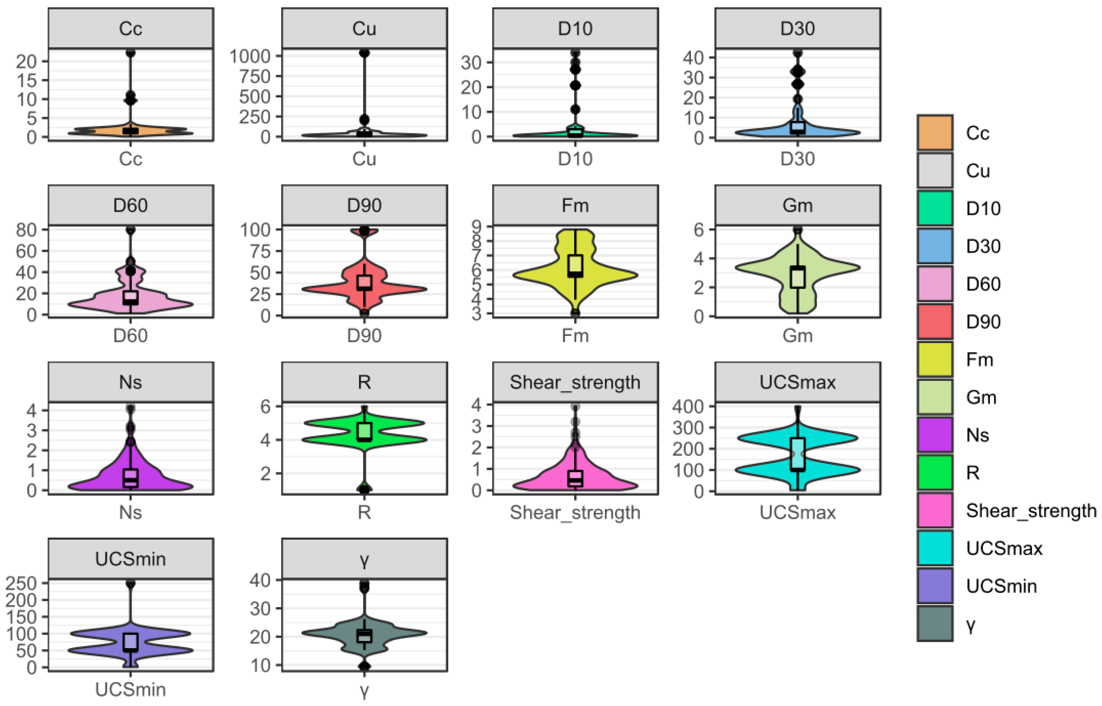
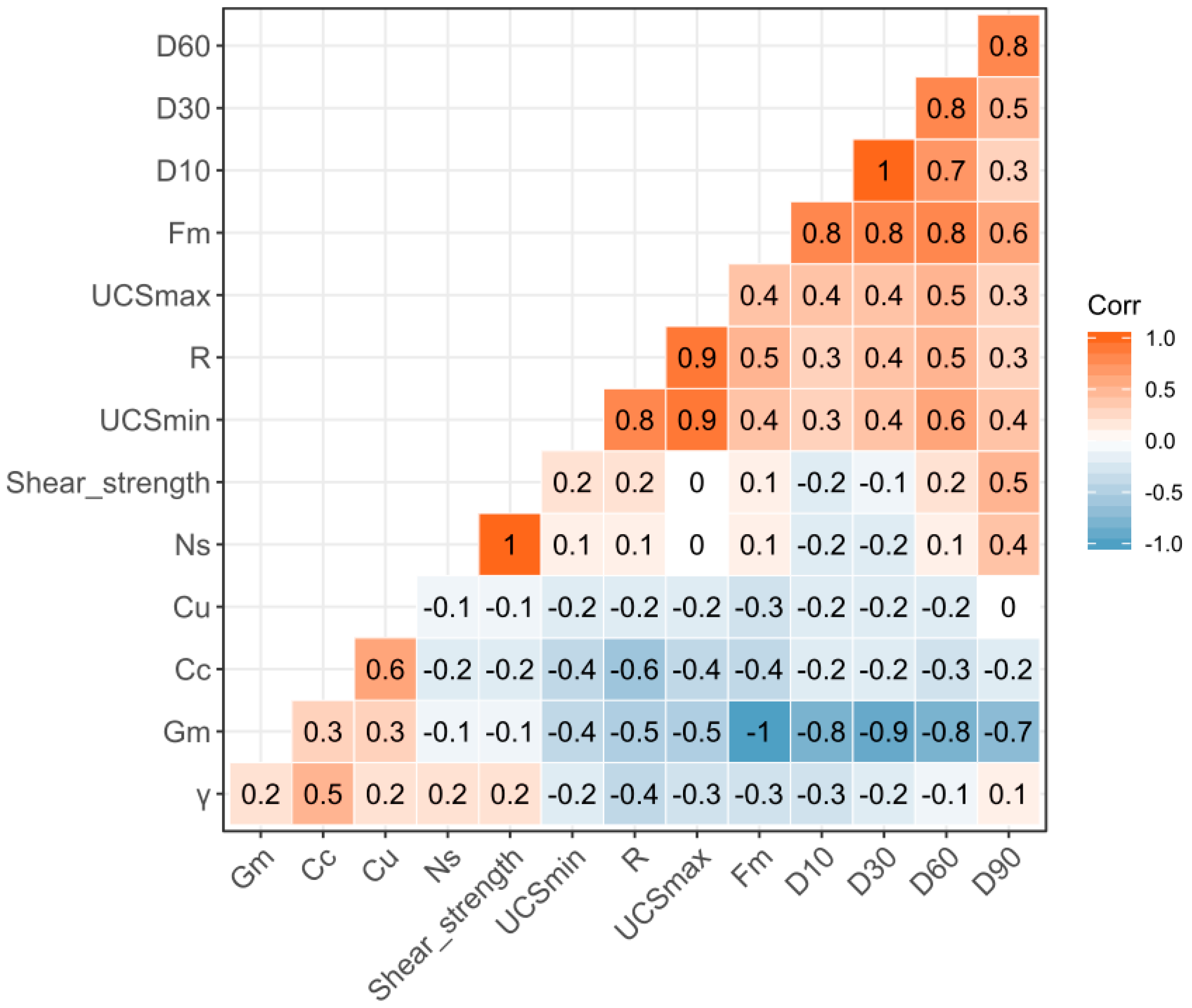
Data quartiles and probability densities (shaded color areas) and outliers (box-and-whisker plots) are illustrated in Figure 1 via violin plots (VIP), which combine density estimates and box plots in displaying the data structure. The top of the plot, the center of the plot and the bottom of the plot show the maximum value, the median value and the minimum value, respectively. The third quartile and the first quartile are represented as the bottom of the thick line and the top of the thick line, respectively, in the center of the VIP. Figure 1 shows the relevant input indicators that are applied to develop the shear strength of the RFM prediction models associated with their mean, range and outputs. The main advantage of the VIP, compared to a box plot, is that the VIP presents the density. A wider VIP corresponds to a higher density. Considering the VIP for Ns in Figure 1 as an example, the minimum and maximum, which are represented by the bottom of the VIP and the top of the VIP, are approximately 0 and 4.5, respectively. The median, which is denoted by a white dot, is approximately 0.5. The highest density occurs for the value 0.3 (i.e., the violin is widest near 0.3), but the high values (between 3 and 4) have a small density (i.e., the pointy top of the VIP near 4). The relationship between the shear strength of RFM and other input indicators is demonstrated in the correlation matrix plot (see Figure 2), which can be observed as the pairwise relationship between two indicators with corresponding correlation coefficients for each indicator. The conclusion that some of the parameters have a relatively satisfactory correlation is obtained. A high parameter of shear strength is correlated with Ns. Barton [1] also noted that the shear strength of rock joints and rockfill exhibits a strong relevance. As demonstrated in Figure 1, some indicators with significant skewness can have an impact on prediction models. In this study, all variables were transformed by the approach of the Box-Cox [32]. Thus, the original data can be conformed to a normal distribution, and the indicators have also been centered and scaled before random forests and Cubist models are conducted.
3.2. Results of Hyper-Parameters Tuning
In the process of the regression of the random forests and Cubist models, an approximate function is determined to predict the value of the output. First, the original datasets of rockfill shear strength are randomly separated to a training set and a test set. In this paper, approximately four-fifths of the available data were randomly chosen to establish the RFM training dataset. One-fifth of the available data were used for testing purpose. The test set was used to evaluate the accuracy of the function and estimate the performance of the regression models.
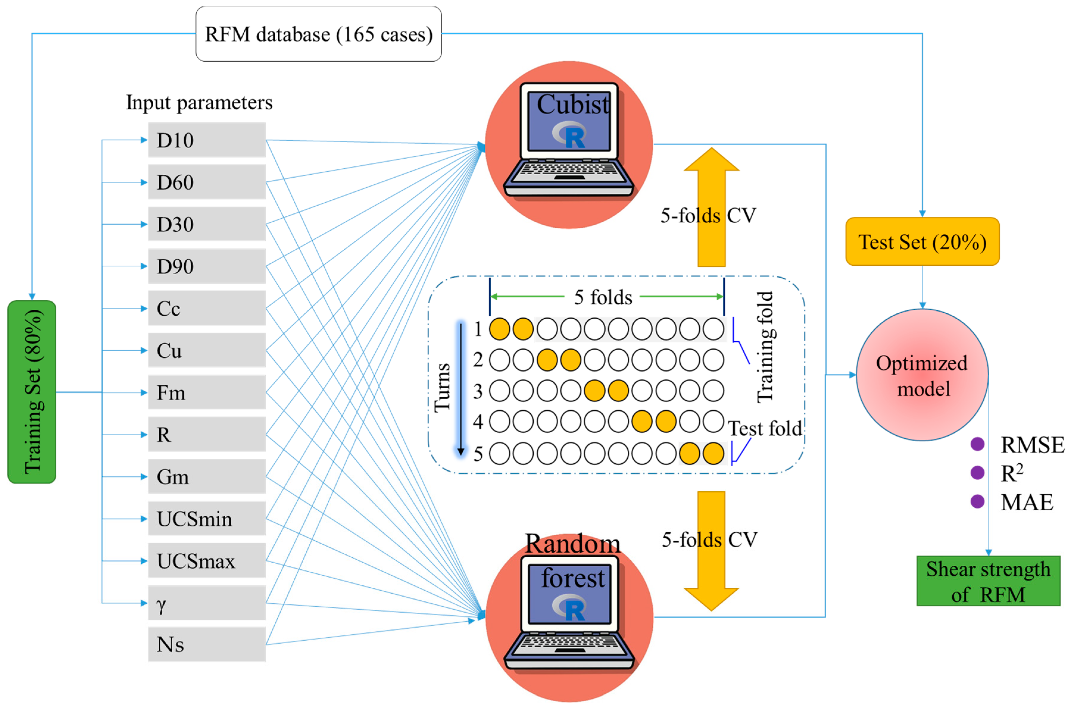
The previously mentioned methods were adopted to predict the shear strength of the RFM in this section. Figure 3 depicts the total procedure for establishing the predictive models and the application of the predictive models to the testing sets. The input parameters (i.e., D10, D30, D60, D90, Cc, Cu, Gm, Fm, R, UCSmin, UCSmax, γ and Ns) in the random forests and Cubist models are the variables that affect the prediction target (shear strength of RFM). Before implementing the experiments, an appropriate division of the RFM datasets is necessary. In supervised regression problems, the RFM datasets are divided into training sets and testing sets. The training set is used for developing RFM estimators and the testing set is used for testing the performance of RFM estimators. The number of training sets determines the performance of RFM estimators. Especially, too few training datasets cannot represent the characteristic of the whole dataset and thus the under-fitting may occur. On the contrast, too large training datasets reduce the capability of generalization of estimators. To conduct the experiments, 165 groups of data on rockfill shear strength are randomly split into a training dataset (133) and a test dataset (32), as shown in Figure 3. To guarantee the same outcome distribution of the whole dataset, the training set is selected from the original datasets with a stratified sampling method [32]. The training set is applied to fit a regression model that is employed to evaluate the parameters of random forests and Cubist regression methods. As previously mentioned, a five-fold CV procedure was implemented to determine the final optimum hyperparameters of random forests and Cubist models. Thus, the original training dataset was randomly divided into five groups, where one-fifth of the data was selected as the testing data, and the remaining four-fifths of the data comprises the training data. For each fold CV procedure, the regression function is established, and a predictive accuracy is obtained, the total five CV procedures are conducted, and the final accuracy is the mean of the previously mentioned accuracy values of the five CV procedures, as demonstrated in Figure 3.
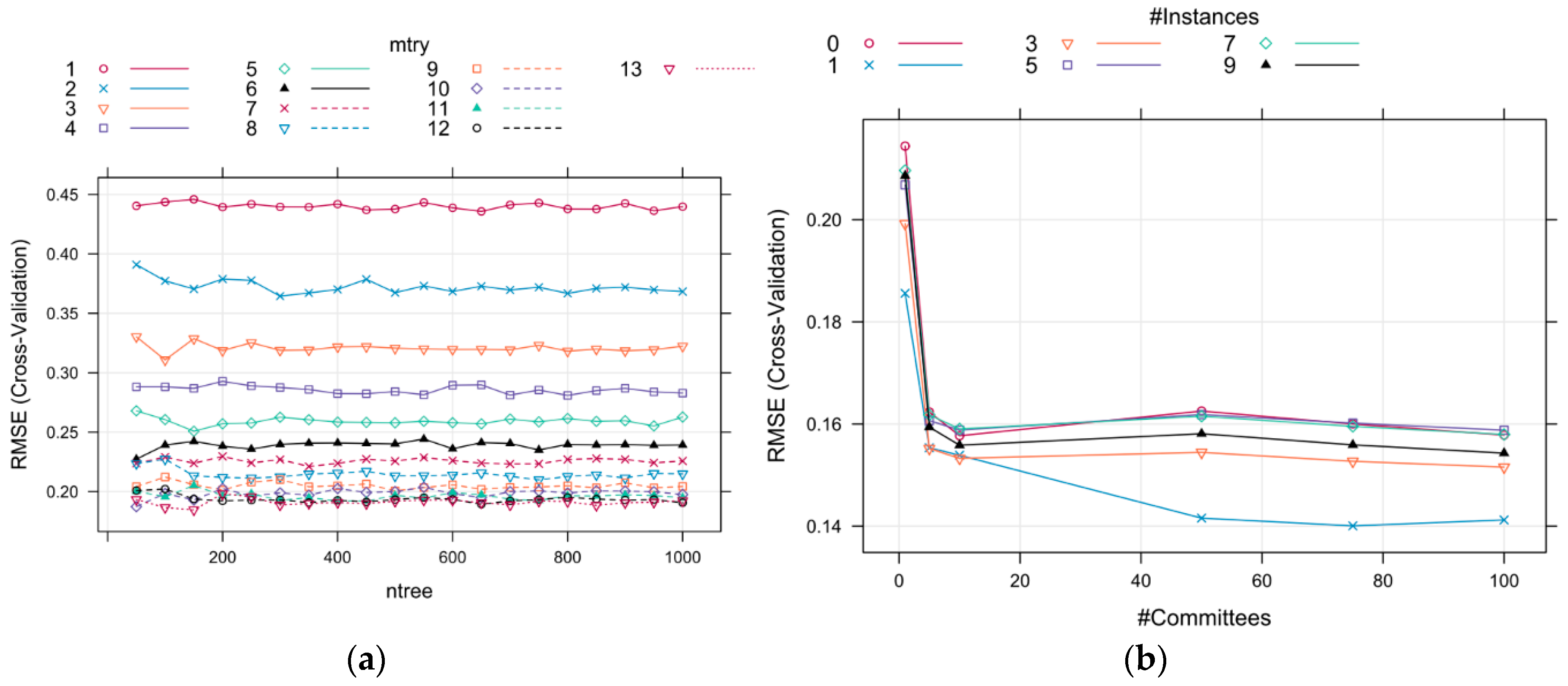
In the application of random forests experiments, the caret package in R was utilized to build a regression model using a Cubist model tree. To investigate the behavior of the random forests hyper-parameters (ntree and mtry), the model was tuned using a relatively fine search grid with CV methods, and the tuning parameters are set as follows: the optimum hyper-parameter mtry is selected in an integer scope of {1,2,3,…,13}, and the optimum hyper-parameter ntree is selected in a scope of [50:1000], incrementing 50 at a time. The smallest value of the RMSE usually indicates the best optimization model. The simplified diagram of the RMSE cross-validated for the random forests is depicted in Figure 4a; the RMSE value of the random forests model is more sensitive to mtry than to ntree. The best optimization values for the random forests model with a 5-fold CV procedure (Figure 4a) were ntree = 150 and mtry = 13. The RMSE, R2 and MAE of the random forests model for 133 sets of training data are 0.1858, 0.9316 and 0.1062, respectively.
Similarly, in the Cubist regression model, which generally has two tweaking parameters that can be fine-tuned [32], committees and neighbors, the tuning parameters are established as follows: the optimum hyper-parameter committees are selected in the scope of {1,5,10,50,75,100} and the optimum hyper-parameter neighbors is selected in the scope of {0,1,3,5,7,9}. To tune the Cubist model over different values of neighbors and committees, the train function in the caret package [50] can be employed to optimize the previously mentioned parameters. In this study, a smaller value of RMSE indicates better optimization results of the Cubist regression model. The relationship between committees and neighbors is shown in Figure 4b. The error does not sharply decrease after the parameter committees attain a value of 10. The finally determined values for the Cubist regression model (Figure 4b) were committees = 75 and neighbors = 1. The RMSE, R2 and MAE of the Cubist model for the training set are 0.1400, 0.9576 and 0.0856, respectively. In addition, the RMSE, R2 and MAE of the predicted values using the linear regression (LR) method [56] are 0.2177, 0.8931 and 0.1317, respectively, for the training data. The RMSE, R2 and MAE of the predicted values using ANN method [20] (delay = 0.1, size = 27) are 0.1875, 0.9168 and 0.1134, respectively, for the training data. The findings reveal that the Cubist model has the ability to capture high nonlinearity and incorporate many parameters.
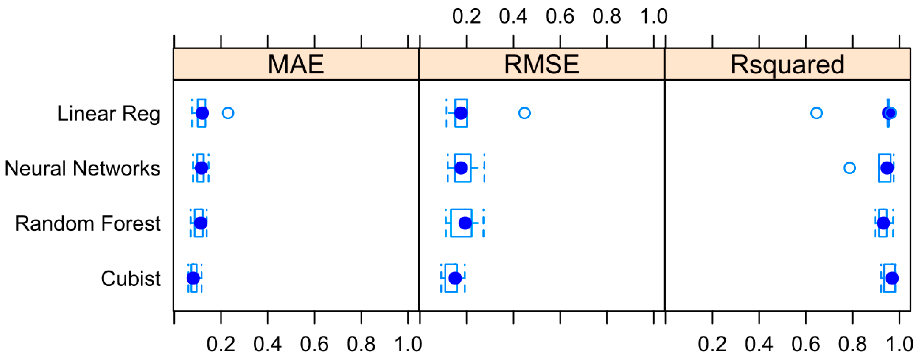
Additionally, Figure 5 shows the result of a comparison of the performance of random forests, Cubist regression, ANN and linear regression algorithms with RMSE, R2 and MAE using a fivefold CV phrase with the training set of R2, RMSE and MAE with its variance, it can be easily observed that the Cubist model yields better performance than Random forests regression model. Compared with the random forests, the difference between lower and upper quartiles in the Cubist model is smaller, while in respect of the variance of accuracies, the random forests model tends to perform better in different iterations.
3.3. Results of Independent Test Set
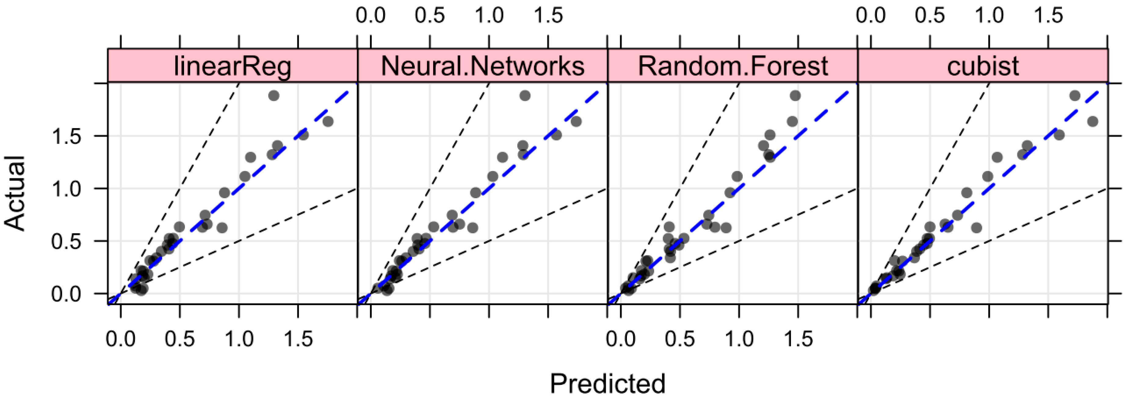
To validate the predictive models based on the predicted and measured (real) values, 32 testing samples were validated by the optimized random forests and Cubist models. Figure 6 and Table 2 illustrate the regression results. Figure 6 shows the actual vs predicted the shear strength of RFM by linear regression, random forests and the Cubist algorithm using test data. Figure 6 suggests that all predicted values by random forests and the Cubist method lie within ± 25% error from the line of perfect agreement. In Figure 6, the RMSE, R2 and MAE between the observed values and predicted values of the random forests model were 0.1133, 0.9548 and 0.0665, respectively, for the test data. The RMSE, R2 and MAE for the predicted values using the Cubist method were 0.0959, 0.9697 and 0.0671, respectively, for the test data. Additionally, the RMSE, R2 and MAE of the predicted values using the conventional multiple linear regression method [56] were 0.1361, 0.9345 and 0.0888, respectively, for the test data. The RMSE, R2 and MAE of the predicted values using the ANN method [20] were 0.1361, 0.9345 and 0.0888, respectively, for the test data. The performance has been improved by random forests and Cubist modeling approaches compared with the conventional multiple linear regression and artificial neural network in terms of R2, RMSE and MAE values (Table 2). In particular, the Cubist model yielded the best result in the section of testing datasets. As a strong tool for modeling the rule-based models, the Cubist model is able to balance the relationship between the predictive accuracy and the requirements of intelligibility.
Although direct measurement of the shear strengths of rockfill materials is a reliable method, efforts should be made to overcome the complexities of the experiment, especially the difficulties of obtaining rock samples from field sites. Different testing procedures for determining the shear strengths of rockfill materials may yield substantial differences in the results, and most rock testing laboratories are not equipped to perform tests for determining the shear strengths of rockfill materials. A possible substitutional method is to study the shear behaviors of rockfill materials using the relationships between the shear parameters and the physicomechanical properties of rockfill materials and develop a prediction method for evaluating the shear strengths of rockfill materials via machine learning approaches. For the given training dataset and regression target, both Cubist regression and random forests show effective prediction ability with the specification of a few tunable model parameters as previously mentioned. As advanced data-driven tools, these two supervised machine learning techniques have the potential for learning the complex interrelationships between explanatory data variables and the target property.
3.4. Variable Importance and Interpretation
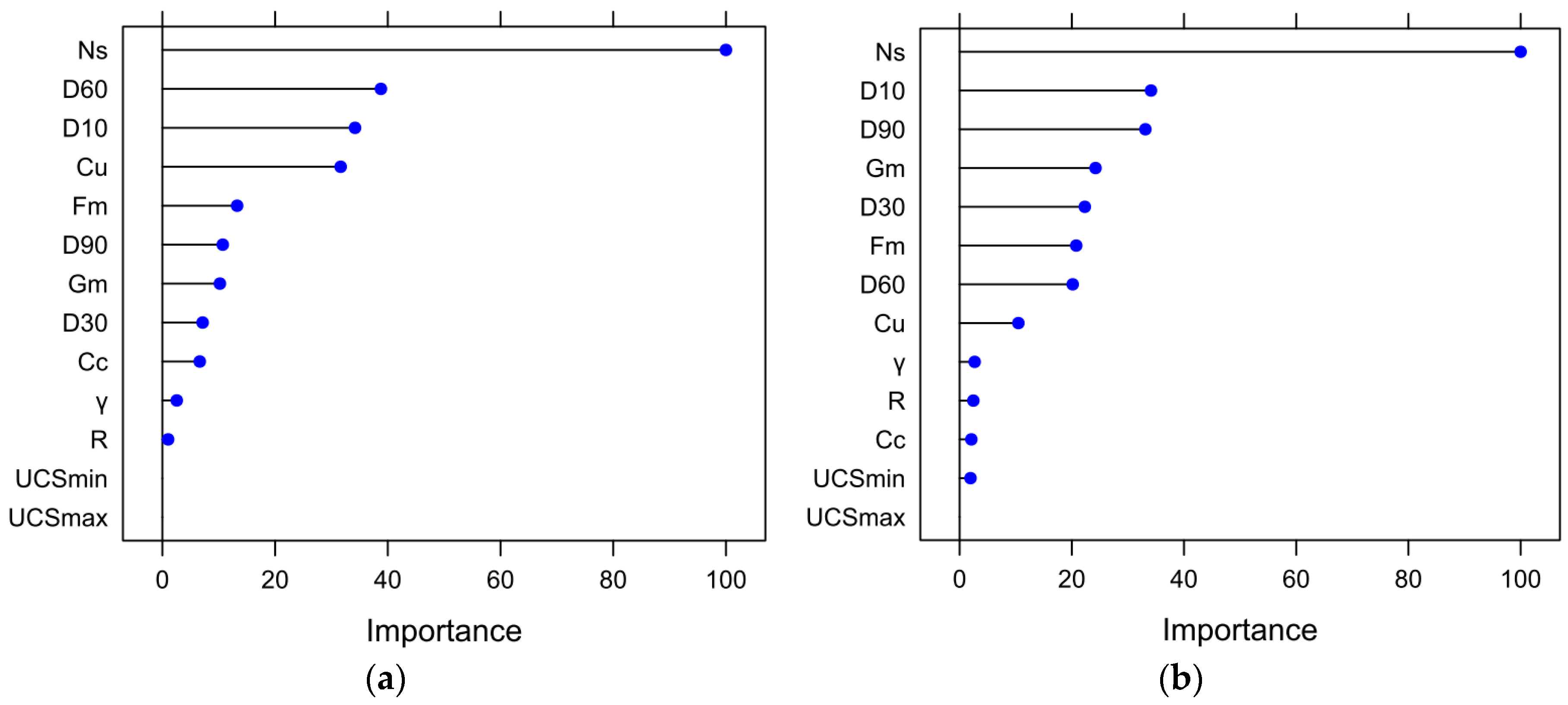
The importance of influencing variables can be individually evaluated by the feature importance to aid in the interpretation of previous results based on the decrease of Gini impurity when a variable is chosen to split a node [32]. The sensitivity analysis of the indicators is conducted to determine the degree of contribution of each variant indicator among all estimation cases. The Cubist model in this database employed the 13 parameters of D10, D30, D60, D90, Cc, Cu, Gm, Fm, R, UCSmin, UCSmax, γ and Ns. The results for the Cubist model are given in Figure 7a, which demonstrates the relative variable importance for the final Cubist model. Among all indicators in the final Cubist model for the prediction of the shear strength of RFM with the given dataset, Ns and D60 are the two most influential parameters, followed by the indicators D10, Cu, Fm, D90, Gm, D30, Cc, γ, R, UCSmin and UCSmax.
Similarly, the random forests model in this database used 13 previously mentioned parameters. Compared with other indicators for the prediction of the shear strength of RFM, Ns and D10 are the two most influential parameters, followed by the indicators D90, Gm, D30, Fm, D60, Cu, γ, R, Cc, UCSmin and UCSmax, as depicted in Figure 7b. Interestingly, the min UCS and max UCS indicators did not contribute to the performance of the proposed models. These results are also consistent with the correlation matrix of the variables that have the highest coefficients for these variables. The findings demonstrated that the Cubist and random forests predictors are more sensitive to the indicators of normal stress and material gradation properties but are not sensitive to min UCS and max UCS. This result implies significant guidance for exploring the characteristics of the shear strength of RFM. Similar research of sensitivity analyses on this topic was also implemented by Kaunda [20], who reported the rankings of the following input parameters: normal stress, minimum particle strength, dry unit weight, 10% passing sieve size, the coefficient of curvature of the particle size distribution, and the coefficient of uniformity of the particle size distribution in decreasing order of significance, which shows agreement with the previously mentioned results. Note that more data about the in-situ shear strength of RFM need to be supplemented to yield more reliable importance scores of random forests and Cubist models for influential variables in future research.
3.5. Limitations
The use of the random forest and Cubist approaches for the shear strength of RFM has limitations that need to be addressed in future research. First, the limitation of the random forest and Cubist approaches is that the datasets are relatively small; only 165 cases are involved in random forest and Cubist modeling. A larger dataset should be analyzed to improve the model’s precision and reliability. Second, other qualitative parameters (i.e., the lithology, the Los Angeles abrasion value) that influences the shear strength of RFM and other hyperparameters of the random forest and Cubist algorithms may exist for improving the performance. Other optimization strategies such as heuristic algorithms [57,58,59,60,61,62,63,64] can obtain the desired results, and many heuristic/hybrid algorithms have been proved to have the potential to significantly reduce the computation time by avoiding exhaustive computation. Third, although regression problems for the shear strength of RFM potential were performed with high accuracy, binary classification problems and multi-output classification problems for the shear strength of RFM analysis have not been investigated in this study. Similar to other machine learning methods, the major disadvantages of random forest and Cubist models are that the resulting tree structure tends to be sensitive to the fitness of the dataset. Due to their “black box” nature, interpretation of the complex relationships between the predictive results and the predictor variables is difficult, and an overfitted condition often occurred. Last, other advanced supervised machine learning techniques that achieve excellent performance in nonlinear relationship modeling, such as support vector machines [55,57] and gradient boosted machines [21,31,32], have not been investigated and compared with the shear strengths of RFM prediction. The optimal prediction result would depend on the size and quality of the dataset. Feature selection is an important step in building a regression model.
4. Conclusions
This paper investigates the potential of random forest and Cubist regression techniques for predicting the shear strength of RFM and identifies useful parameters that affect the prediction of rockfill shear strength. This study concluded that Cubist and random forest regression algorithms are more suitable for predicting the shear strength of RFM compared with conventional multiple linear regression and ANN in terms of explanatory value and error. In this study, the Cubist model (RMSE =0.0959, R2 = 0.9697 and MAE = 0.0671) appeared to be superior to random forests (RMSE = 0.1133, R2 = 0.9548 and MAE = 0.0665) with this type of dataset but random forests can achieve reasonable prediction accuracies in some cases. Another important conclusion of this study is that Cubist and random forest regression algorithms can effectively identify useful input parameters that affect the shear strength of RFM. Supervised machine learning based approaches are very sensitive to the quality and type of data, and their performance may change depending on the dataset, the quality and number of training datasets and the scale at which the experiments are conducted. Future studies can explore whether the accuracy can be improved by increasing or reducing the training dataset to validate the proposed model, by adjusting/tuning the hyperparameters of the algorithms or implementing a new predictive model. Additional experiments using a larger number of datasets are suggested to estimate the performance of the random forest and Cubist algorithms in forecasting RFM values that exceed the range of the pre-existing training dataset.
Author Contributions
Conceptualization, J.Z.; Data curation, E.L.; Formal analysis, C.L.; Supervision, H.W.; Writing—review and editing, J.Z., Q.Q. and D.J.A.
Funding
This research was funded by the National Science Foundation of China (41807259, 51504082), the Natural Science Foundation of Hunan Province (2018JJ3693), the China Postdoctoral Science Foundation funded project (2017M622610) and the Shenghua Lieying Program of Central South University (Principle Investigator: Jian Zhou).
Conflicts of Interest
The authors confirm that this article content has no conflict of interest.
References
- Barton, N. Shear strength criteria for rock, rock joints, rockfill and rock masses: Problems and some solutions. J. Rock Mech. Geotech. Eng. 2013, 5, 249–261. [Google Scholar] [CrossRef] [Green Version]
- Honkanadavar, N.P.; Gupta, S.L. Prediction of shear strength parameters for prototype riverbed rockfill material using index properties. In Proceedings of the Indian Geotechnical Conference, New Delhi, India, 16–18 December 2010; Indian Geotechnical Society: New Delhi, India, 2010; pp. 335–338. [Google Scholar]
- Araei, A.A.; Soroush, A.; Rayhani, M. Large scale triaxial testing and numerical modeling of rounded and angular rockfill materials. Sci. Iran. Trans. A Civ. Eng. 2010, 17, 169–183. [Google Scholar]
- Varadarajan, A.; Sharma, K.G.; Venkatachalam, K.; Gupata, A.K. Testing and modeling two rockfill materials. J. Geotech. Geoenviron. Eng. 2003, 129, 206–218. [Google Scholar] [CrossRef]
- Pankaj, S.; Mahure, N.V.; Gupta, S.L.; Sandeep, D.; Devender, S. Estimation of shear strength of prototype rockfill materials. Int. J. Eng. 2013, 2, 421–426. [Google Scholar]
- Leps, T.M. Review of Shearing Strength of rockfill. J. Soil Mech. Found. Eng. Div. 1970, 96, 1159–1170. [Google Scholar]
- Liu, S.H. Application of in situ direct shear device to shear strength measurement of rockfill materials. Water Sci. Eng. 2009, 2, 48–57. [Google Scholar]
- Linero, S.; Palma, C.; Apablaza, R. Geotechnical characterization of waste material in very high dumps with large scale triaxial testing. In Proceedings of the International Symposium on Rock Slope Stability in Open Pit Mining and Civil Engineering, Perth, Australia, 12–14 September 2007; Australian Centre for Geomechanics: Perth, Australia, 2007; pp. 59–75. [Google Scholar]
- Xu, M.; Song, E. Numerical simulation of the shear behavior of rockfills. Comput. Geotech. 2009, 36, 1259–1264. [Google Scholar] [CrossRef]
- Frossard, E.; Hu, W.; Dano, C.; Hicher, P.Y. Rockfill shear strength evaluation: A rational method based on size effects. Geotechnique 2012, 62, 415. [Google Scholar] [CrossRef]
- Armaghani, D.J.; Hajihassani, M.; Bejarbaneh, B.Y.; Marto, A.; Mohamad, E.T. Indirect measure of shale shear strength parameters by means of rock index tests through an optimized artificial neural network. Measurement 2014, 55, 487–498. [Google Scholar] [CrossRef]
- Gong, F.Q.; Luo, Y.; Li, X.B.; Si, X.F.; Tao, M. Experimental simulation investigation on rockburst induced by spalling failure in deep circular tunnels. Tunn. Undergr. Space Technol. 2018, 81, 413–427. [Google Scholar] [CrossRef]
- Tao, M.; Zhao, H.T.; Li, X.B.; Cao, W.Z. Failure characteristics and stress distribution of pre-stressed rock specimen with circular cavity subjected to dynamic loading. Tunn. Undergr. Space Technol. 2018, 81, 1–15. [Google Scholar] [CrossRef]
- Tao, M.; Ma, A.; Cao, W.Z.; Li, X.B.; Gong, F.Q. Dynamic response of pre-stressed rock with a circular cavity subject to transient loading. Int. J. Rock Mech. Min. Sci. 2017, 99, 1–8. [Google Scholar] [CrossRef]
- Qiao, Q.Q.; Nemcik, J.; Porter, I. A new approach for determination of the shear bond strength of thin spray-on liners. Int. J. Rock Mech. Min. Sci. 2015, 73, 54–61. [Google Scholar] [CrossRef]
- Wang, Y.X.; Shan, S.B.; Zhang, C.; Guo, P.P. Seismic response of tunnel lining structure in a thick expansive soil stratum. Tunn. Undergr. Space Technol. 2019, 88, 250–259. [Google Scholar] [CrossRef]
- Wang, Y.; Guo, P.; Dai, F.; Li, X.; Zhao, Y.; Liu, Y. Behavior and modeling of fiber-reinforced clay under triaxial compression by combining the superposition method with the energy-based homogenization technique. Int. J. Geomech. 2018, 18, 04018172. [Google Scholar] [CrossRef]
- Kim, Y.S.; Kim, B.T. Prediction of relative crest settlement of concrete-faced rockfill dams analyzed using an artificial neural network model. Comput. Geotech. 2008, 35, 313–322. [Google Scholar] [CrossRef]
- Araei, A.A. Artificial neural networks for modeling drained monotonic behavior of rockfill materials. Int. J. Geomech. 2013, 14, 04014005. [Google Scholar] [CrossRef]
- Kaunda, R. Predicting shear strengths of mine waste rock dumps and rock fill dams using artificial neural networks. Int. J. Min. Miner. Eng. 2015, 6, 139–171. [Google Scholar] [CrossRef]
- Zhou, J.; Li, X.B.; Mitri, H.S. Classification of rockburst in underground projects: Comparison of ten supervised learning methods. J. Comput. Civ. Eng. 2016, 30, 04016003. [Google Scholar] [CrossRef]
- Asteris, P.G.; Plevris, V. Anisotropic masonry failure criterion using artificial neural networks. Neural Comput. Appl. 2017, 28, 2207–2229. [Google Scholar] [CrossRef]
- Asteris, P.G.; Kolovos, K.G.; Douvika, M.G.; Roinos, K. Prediction of self-compacting concrete strength using artificial neural networks. Eur. J. Environ. Civ. Eng. 2016, 20, s102–s122. [Google Scholar] [CrossRef]
- Zhou, J.; Li, X.; Mitri, H.S. Evaluation method of rockburst: State-of-the-art literature review. Tunn. Undergr. Space Technol. 2018, 81, 632–659. [Google Scholar] [CrossRef]
- Koopialipoor, M.; Fallah, A.; Armaghani, D.J.; Azizi, A.; Mohamad, E.T. Three hybrid intelligent models in estimating flyrock distance resulting from blasting. Eng. Comput. 2019, 35, 243–256. [Google Scholar] [CrossRef]
- Asteris, P.G.; Tsaris, A.K.; Cavaleri, L.; Repapis, C.C.; Papalou, A.; Di Trapani, F.; Karypidis, D.F. Prediction of the fundamental period of infilled RC frame structures using artificial neural networks. Comput. Intell. Neurosci. 2016, 2016, 5104907. [Google Scholar] [CrossRef]
- Koopialipoor, M.; Armaghani, D.J.; Hedayat, A.; Marto, A.; Gordan, B. Applying various hybrid intelligent systems to evaluate and predict slope stability under static and dynamic conditions. Soft Comput. 2018. [Google Scholar] [CrossRef]
- Breiman, L. Random forests. Mach. Learn. 2001, 45, 5–32. [Google Scholar] [CrossRef]
- Adusumilli, S.; Bhatt, D.; Wang, H.; Bhattacharya, P.; Devabhaktuni, V. A low-cost INS/GPS integration methodology based on random forest regression. Expert Syst. Appl. 2013, 40, 4653–4659. [Google Scholar] [CrossRef]
- Zhou, J.; Shi, X.Z.; Du, K.; Qiu, X.Y.; Li, X.B.; Mitri, H.S. Feasibility of random-forest approach for prediction of ground settlements induced by the construction of a shield-driven tunnel. Int. J. Geomech. 2017, 17, 04016129. [Google Scholar] [CrossRef]
- Zhou, J.; Li, X.; Mitri, H.S. Comparative performance of six supervised learning methods for the development of models of hard rock pillar stability prediction. Nat. Hazards 2015, 79, 291–316. [Google Scholar] [CrossRef]
- Kuhn, M.; Johnson, K. Applied Predictive Modeling; Springer: New York, NY, USA, 2013. [Google Scholar]
- Quinlan, R. Learning with continuous classes. In Proceedings of the 5th Australian Joint Conference on Artificial Intelligence, Hobart, Australia, 16–18 November 1992; pp. 343–348. [Google Scholar]
- Quinlan, R. Combining instance based and model based learning. In Proceedings of the Tenth International Conference on Machine Learning, Amherst, MA, USA, 27–29 June 1993; pp. 236–243. [Google Scholar]
- Wang, Y.; Witten, I. Inducing model trees for continuous classes. In Proceedings of the Ninth European Conference on Machine Learning, Prague, Czech Republic, 23–25 April 199; pp. 128–137.
- Kuhn, M.; Weston, S.; Keefer, C.; Coulter, N.; Quinlan, R. Cubist: Rule-and Instance-based Regression Modeling, R package version 0.0.18; CRAN: Vienna, Austria, 2014. [Google Scholar]
- Haselsteiner, R.; Pamuk, R.; Ersoy, B. Aspects concerning the shear strength of rockfill material in rockfill dam engineering. Geotechnik 2017, 40, 193–203. [Google Scholar] [CrossRef]
- Douglas, K.J. The Shear Strength of Rock Masses. Ph.D. Thesis, University of New South Wales, Sydney, Australia, 2002. [Google Scholar]
- Ghanbari, A.; Sadeghpour, A.H.; Mohamadzadeh, H.; Mohamadzadeh, M. An experimental study on the behavior of rockfill materials using large scale tests. Electron. J. Geotech. Eng. 2008, 13, 1–16. [Google Scholar]
- Charles, J.A.; Watts, K.S. The influence of confining pressure on the shear strength of compacted rockfill. Geotechnique 1980, 30, 353–367. [Google Scholar] [CrossRef]
- Marachi, N.D.; Chan, C.K.; Seed, H.B.; Duncan, J.M. Strength and Deformation Characteristics of Rockfill Materials; Report No. TE-69-5; Department of Civil Engineering, University of California: Berkeley, CA, USA, 1969. [Google Scholar]
- Hudson, S.B.; Waller, H.F. Evaluation of Construction Control Procedures: Aggregate Gradation Variations and Effects; NCHRP Report; Transportation research Board: Washington, DC, USA, 1969; Volume 69. [Google Scholar]
- Lusher, S.M. Prediction of the Resilient Modulus of Unbound Granular Base and Subbase Materials based on the California Bearing Ratio and Other Test Data. Ph.D. Thesis, University of Missouri—Rolla, Rolla, MO, USA, 2004. [Google Scholar]
- Indraratna, B.; Wijewardena, L.S.S.; Balasubramaniam, A.S. Large-scale triaxial testing of greywacke rockfill. Geotechnique 1993, 43, 37–51. [Google Scholar] [CrossRef]
- Brown, E.T. (Ed.) Rock Characterization Testing and Monitoring; ISRM suggested methods; Pergamon Press: Oxford, UK, 1981. [Google Scholar]
- Zhou, J. Strainburst Prediction and Spalling Depth Estimation Using Supervised Learning Methods. Ph.D. Thesis, Central South University, Changsha, China, 2015. [Google Scholar]
- Kohavi, R. A study of cross-validation and bootstrap for accuracy estimation and model selection. In Proceedings of the International Joint Conference on Artificial Intelligence, Montreal, QC, Canada, 20–25 August 1995; pp. 1137–1145. [Google Scholar]
- Rodriguez, J.D.; Perez, A.; Lozano, J.A. Sensitivity analysis of k-fold cross validation in prediction error estimation. IEEE Trans. Pattern Anal. Mach. Intell. 2010, 32, 569–575. [Google Scholar] [CrossRef] [PubMed]
- Wong, T.T. Performance evaluation of classification algorithms by k-fold and leave-one-out cross validation. Pattern Recognit. 2015, 48, 2839–2846. [Google Scholar] [CrossRef]
- Kuhn, M. Building predictive models in R using the caret package. J. Stat. Softw. 2008, 28, 1–26. [Google Scholar] [CrossRef]
- Ferlito, S.; Adinolfi, G.; Graditi, G. Comparative analysis of data-driven methods online and offline trained to the forecasting of grid-connected photovoltaic plant production. Appl. Energy 2017, 205, 116–129. [Google Scholar] [CrossRef]
- Zhou, J.; Li, E.; Wang, M.; Chen, X.; Shi, X.; Jiang, L. Feasibility of stochastic gradient boosting approach for evaluating seismic liquefaction potential based on SPT and CPT Case Histories. J. Perform. Constr. Facil. 2019, 33, 04019024. [Google Scholar] [CrossRef]
- Noi, P.; Degener, J.; Kappas, M. Comparison of multiple linear regression, cubist regression, and random forest algorithms to estimate daily air surface temperature from dynamic combinations of MODIS LST data. Remote Sens. 2017, 9, 398. [Google Scholar] [CrossRef]
- R Core Team. R: A Language and Environment for Statistical Computing; R Foundation for Statistical Computing: Vienna, Austria, 2013; ISBN 3-900051-07-0. Available online: https://www.R-project.org/ (accessed on 31 May 2017).
- Shi, X.Z.; Zhou, J.; Wu, B.B.; Huang, D.; Wei, W. Support vector machines approach to mean particle size of rock fragmentation due to bench blasting prediction. Trans. Nonferr. Met. Soc. China 2012, 22, 432–441. [Google Scholar] [CrossRef]
- Zhou, J.; Li, X.B. Evaluating the thickness of broken rock zone for deep roadways using nonlinear SVMs and multiple linear regression model. Procedia Eng. 2011, 26, 972–981. [Google Scholar] [CrossRef]
- Zhou, J.; Li, X.B.; Shi, X.Z. Long-term prediction model of rockburst in underground openings using heuristic algorithms and support vector machines. Saf. Sci. 2012, 50, 629–644. [Google Scholar] [CrossRef]
- Hajihassani, M.; Armaghani, D.J.; Monjezi, M.; Mohamad, E.T.; Marto, A. Blast-induced air and ground vibration prediction: A particle swarm optimization-based artificial neural network approach. Environ. Earth Sc. 2015, 74, 2799–2817. [Google Scholar] [CrossRef]
- Zhou, J.; Nekouie, A.; Arslan, C.A.; Pham, B.T.; Hasanipanah, M. Novel approach for forecasting the blast-induced AOp using a hybrid fuzzy system and firefly algorithm. Eng. Comput. 2019. [Google Scholar] [CrossRef]
- Hasanipanah, M.; Armaghani, D.J.; Amnieh, H.B.; Majid MZ, A.; Tahir, M.M. Application of PSO to develop a powerful equation for prediction of flyrock due to blasting. Neural Comput. Appl. 2017, 28, 1043–1050. [Google Scholar] [CrossRef]
- Chen, H.; Asteris, P.G.; Armaghani, D.J.; Gordan, B.; Pham, B.T. Assessing dynamic conditions of the retaining wall using two hybrid intelligent models. Appl. Sci. 2019, 9, 1042. [Google Scholar] [CrossRef]
- Zhou, J.; Aghili, N.; Ghaleini, E.N.; Bui, D.T.; Tahir, M.M.; Koopialipoor, M. A Monte Carlo simulation approach for effective assessment of flyrock based on intelligent system of neural network. Eng. Comput. 2019. [Google Scholar] [CrossRef]
- Asteris, P.G.; Nozhati, S.; Nikoo, M.; Cavaleri, L.; Nikoo, M. Krill herd algorithm-based neural network in structural seismic reliability evaluation. Mech. Adv. Mater. Struct. 2018. [Google Scholar] [CrossRef]
- Asteris, P.G.; Nikoo, M. Artificial bee colony-based neural network for the prediction of the fundamental period of infilled frame structures. Neural Comput. Appl. 2019. [Google Scholar] [CrossRef]
Figure 1.
Original data visualization with violin plots.

Figure 2.
Correlation matrix plot of the original database.

Figure 3.
Illustration of the total procedure for the evaluation of the shear strength of RFM using the proposed methods.
Figure 3.
Illustration of the total procedure for the evaluation of the shear strength of RFM using the proposed methods.

Figure 4.
Fivefold cross-validated RMSE profiles for determining the optimal tuning parameters: (a) Random forests model, and (b) Cubist model.
Figure 4.
Fivefold cross-validated RMSE profiles for determining the optimal tuning parameters: (a) Random forests model, and (b) Cubist model.

Figure 5.
Comparison of the performance of the four algorithms with the MAE, RMSE and R2 metrics.

Figure 6.
Error of the shear strength of RFM for the testing set.

Figure 7.
Variable importance scores for the 13 predictors in the proposed models for shear strength of RFM: (a) Cubist model, and (b) random forests model.
Figure 7.
Variable importance scores for the 13 predictors in the proposed models for shear strength of RFM: (a) Cubist model, and (b) random forests model.


Table 1.
Explanation of input and output variables.
| Inputs and outputs | Variable form in model | Description | Range |
|---|---|---|---|
| Inputs variables | D10 (mm) | 10% percent passing sieve sizes | 0.01–33.90 |
| D30 (mm) | 30% percent passing sieve sizes | 0.56–42.40 | |
| D60 (mm) | 60% percent passing sieve sizes | 1.2–80.1 | |
| D90 (mm) | 90% percent passing sieve sizes | 2.6–100.0 | |
| Cc | Coefficients of uniformity | 0.10–22.27 | |
| Cu | Curvature | 1.36–1040.00 | |
| Gm | Gradation modulus | 0.2–6.0 | |
| Fm | Fineness modulus | 3.0–8.8 | |
| R | ISRM hardness rating | 1–6 | |
| UCSmin (Mpa) | Minimum uniaxial compression strength of group | 1–250 | |
| UCSmax (Mpa) | Maximum uniaxial compression strength of group | 5–400 | |
| γ (kN/m³) | Dry unit weight | 9.3195–38.900 | |
| Ns (Mpa) | Normal stress | 0.01–33.90 | |
| Output variable | Shear strength (Mpa) | Shear strength of RFM | 0.56–42.40 |
Table 2.
The performance of different prediction models for test data.
| Model | R2 | RMSE | MAE |
|---|---|---|---|
| Linear regression | 0.9345 | 0.1361 | 0.0888 |
| Cubist | 0.9645 | 0.0975 | 0.0644 |
| Artificial neural network | 0.9386 | 0.1320 | 0.0841 |
| Random forest | 0.9523 | 0.1282 | 0.0860 |
© 2019 by the authors. Licensee MDPI, Basel, Switzerland. This article is an open access article distributed under the terms and conditions of the Creative Commons Attribution (CC BY) license (http://creativecommons.org/licenses/by/4.0/).
Share and Cite
MDPI and ACS Style
Zhou, J.; Li, E.; Wei, H.; Li, C.; Qiao, Q.; Armaghani, D.J. Random Forests and Cubist Algorithms for Predicting Shear Strengths of Rockfill Materials. Appl. Sci. 2019, 9, 1621. https://doi.org/10.3390/app9081621
AMA Style
Zhou J, Li E, Wei H, Li C, Qiao Q, Armaghani DJ. Random Forests and Cubist Algorithms for Predicting Shear Strengths of Rockfill Materials. Applied Sciences. 2019; 9(8):1621. https://doi.org/10.3390/app9081621
Chicago/Turabian StyleZhou, Jian, Enming Li, Haixia Wei, Chuanqi Li, Qiuqiu Qiao, and Danial Jahed Armaghani. 2019. "Random Forests and Cubist Algorithms for Predicting Shear Strengths of Rockfill Materials" Applied Sciences 9, no. 8: 1621. https://doi.org/10.3390/app9081621
Note that from the first issue of 2016, this journal uses article numbers instead of page numbers. See further details here.