Article

Evolutionary Algorithms to Optimize Task Scheduling Problem for the IoT Based Bag-of-Tasks Application in Cloud–Fog Computing Environment

1
School of Information and Communication Technology, Hanoi University of Science and Technology, 1 Dai Co Viet Street, Hai Ba Trung District, Hanoi 100000, Vietnam
2
School of Computer Science and Engineering, Nanyang Technological University, 50 Nanyang avenue, Singapore 639798, Singapore
3
Faculty of Information Technology, University of Transport Technology, 54 Trieu Khuc Street, Thanh Xuan District, Hanoi 100000, Vietnam
*
Author to whom correspondence should be addressed.
Appl. Sci. 2019, 9(9), 1730; https://doi.org/10.3390/app9091730
Submission received: 28 February 2019 / Revised: 26 March 2019 / Accepted: 17 April 2019 / Published: 26 April 2019
(This article belongs to the Special Issue Edge Computing Applications in IoT)

Abstract

:
In recent years, constant developments in Internet of Things (IoT) generate large amounts of data, which put pressure on Cloud computing’s infrastructure. The proposed Fog computing architecture is considered the next generation of Cloud Computing for meeting the requirements posed by the device network of IoT. One of the obstacles of Fog Computing is distribution of computing resources to minimize completion time and operating cost. The following study introduces a new approach to optimize task scheduling problem for Bag-of-Tasks applications in Cloud–Fog environment in terms of execution time and operating costs. The proposed algorithm named TCaS was tested on 11 datasets varying in size. The experimental results show an improvement of 15.11% compared to the Bee Life Algorithm (BLA) and 11.04% compared to Modified Particle Swarm Optimization (MPSO), while achieving balance between completing time and operating cost.

1. Introduction

Recently, Internet of Things (IoT) has become one of the major revolutions in the information and communication technology industry. With IoT, Internet connection extends beyond traditional smart devices such as smartphones and tablets to a diverse range of devices and things (sensors, machines, vehicles, etc.), to accomplish many different applications and services such as: health care, medical treatment, traffic control, energy management, vehicle networks, etc. This produces a huge amount of data that need to be stored, processed and analyzed to obtain valuable information to meet user’s goals and needs. In addition, the number and scale of applications and services are also increasing rapidly, which requires processing capability that even the most powerful smart devices cannot currently meet. The Cloud environment, which is known as a large resource center that allows ubiquitous access to share and provide resources to users flexibly through virtualization mechanism, can be a potential platform to support IoT developments. Restrictions of existing smart devices (battery life, processing power, storage capacity, and network resources) can be minimized by taking time-consuming and resource-intensive tasks to a powerful computing platform such as Cloud computing while leaving the simple tasks for the smart devices to handle.
However, when combining IoT and Cloud computing, new problems emerge. According to Information Handling Services (IHS) Markit, the IoT market will grow from 15.4 billion devices installed in 2015 to 30.7 billion devices in 2020 and this figure in 2025 will rise to 75.4 billion. With this dramatic increase in number of connected devices, the Cloud architecture with traditional centralized processing characteristics (in which computing and storage resources are gathered and placed in several data centers) will be unable to meet the requirements of IoT applications. The main reason is due to the long distance between the Cloud and IoT devices. Massive flow of data sent by IoT devices to the Cloud via the Internet will result in congestion, especially at bottlenecks, while also creating burden on network performance and bandwidth. The delay in transmission leads to degraded Quality of Service (QoS), which has detrimental effect on the user’s experience, since one of the properties of IoT applications is latency sensitivity. Moreover, constant connection to the Cloud is not always available for IoT devices, simply because it is very expensive. On the other hand, thanks to advances in both hardware and software technologies, many devices on the edge of the network (routers, gateways, workstations, personal computers, etc.) have more and more processing, storage and communication capabilities.
Fog computing [1], first proposed by Cisco, represents a new model of Cloud computing, which can transform a network edge into a distributed computing infrastructure capable of implementing IoT applications. The concept of Fog Computing is to extend Cloud computing closer to the IoT devices that produce and consume data, which in turn brings processing and storage resources closer to users. Rather than pushing all processing operation to the Cloud, Fog Computing aims to handle part of workloads produced by applications on devices close to the network near the users, which are called Fog servers or Fog nodes. These devices can be deployed anywhere that has network connectivity: factories, commercial centers, on power poles, next to railways, inside vehicles, etc. Any device that has computing, storage and networking capabilities can be considered a Fog Node: controllers, switches, routers, embedded servers, surveillance cameras, etc. By placing resources at the edge of the network, the time it takes for data to reach a processing station becomes negligible, therefore the tasks are optimized for transmission time. However, processing capability of a Fog Node is restricted, thus small tasks or processing requests with short delay will be prioritized to be processed on Fog Computing infrastructure, while tasks that have delay-tolerant and tasks of larger scale will still be pushed to Cloud layers. Eventually, Fog computing complements the Cloud to form a new computing paradigm, Cloud–Fog computing.
The Cloud–Fog computing model has numerous advantages, including reduced latency, reduced network traffic and increased energy efficiency, however, this new model also comes with a set of challenges. One of them is resource allocation and tasks scheduling. A highly distributed system such as Cloud–Fog computing is an ideal platform to deploy Bag-of-Tasks (BoT) applications, which are those parallel applications whose tasks are independent to each other. BoT applications appear in many scenarios, including data mining, massive searches (such as key breaking), fractal calculations, computational biology [2], computer imaging [3], video encoding/decoding, and various other IoT applications. The main challenge is scheduling tasks in the pool of processing nodes including cloud nodes (such as servers or virtual machines) and Fog nodes. The goal of task scheduling in Cloud–Fog system is aimed at the benefit of users or service providers. On the users side, they are concerned about some criteria of makespan, budget, deadline, security, and cost. On the other hand, the purpose of the service providers is load balancing, resource utilization, and energy efficiency. To guarantee the QoS, response time plays an important role when directly influencing the user’s experience. In addition, the implementation cost is also an aspect that users are very interested. A task schedule, which minimizes completion time and saves monetary cost, will satisfy Service Level Agreement (SLA) signed with users.
In this paper, we concentrate on task scheduling problem in Cloud–Fog environment, a highly distributed computing platform, for processing large-scale BoT applications. A Time–Cost aware Scheduling (TCaS) algorithm is proposed to solve this problem. The major objective of the TCaS algorithm is to achieve a good trade-off between execution time and monetary cost to complete a bag of tasks in Cloud–Fog system. In addition, this algorithm can flexibly adapt with the requires of various users in which someone wants to prioritize the execution time at current time and others have a desire that their tasks are completed with a tight budget. Our approach was experimentally evaluated and compared with Bee Life Algorithm (BLA) [4], Modified Particle Swarm Optimization (MPSO) and Round Robin (RR) algorithm on many datasets with various size. The results prove that the proposed algorithm achieved better QoS and was more optimal in balance between time and cost efficiency than BLA.
The rest of the article is organized as follows. In Section 2, the related works are presented. Section 3 specifies the mathematical model for the task scheduling problem in the Cloud–Fog computing environment. Section 4 presents our proposed algorithm in detail. Experimental results are given in Section 5. Finally, Section 6 concludes the article and future works are discussed.

2. Related Works

2.1. Fog Computing with IoT

The centralized Cloud architecture is facing a number of challenges from IoT applications. For example, IoT cannot support applications that require low latency and real-time applications such as connected vehicles [1], smart traffic lights [5], etc. Fog computing can solve these challenges. Table 1 summarizes differences between Cloud and Fog computing.
Fog computing can help address Internet of Things challenges according to Chiang and Zhang [6]
  • Latency constraints: Fog Computing is often the best candidate when it comes to dealing with strict timing requirements of many IoT systems such as data analyzing, data managing and other latency-restrictive tasks close to end users.
  • Network bandwidth constraints: Fog Computing allows data sent and received from the end users to the Cloud to be processed hierarchically so that the trade-off between application demands and available networking and computing resources is considered. This also optimizes data usage, reducing the amount needed to be sent to the Cloud.
  • Resource-limited devices: Resource-intensive tasks can be performed by Fog instead of resource-limited devices when they cannot be sent to the Cloud, which reduces these devices’s complexity, maintenance cost, and energy consumption.
  • Uninterrupted services with sporadic connectivity to the cloud: A Fog system can function independently to maintain constant services despite having sporadic network connectivity to the Cloud.
  • IoT security challenges: A Fog system is capable of the following: (1) acting as proxies for resource-limited devices of which security credentials and software can be managed and updated; (2) performing numerous security protocols on behalf of the resource-limited devices, to make up for the lack of security functionality on these devices; (3) overseeing the security status of devices in close proximity; and (4) using gathered information and context to identify threats promptly.
This section describes articles on the convergence between IoT and Fog computing. Fog computing is still a recent research topic, thus concrete solutions to support this computer paradigm are lacking. In this section, we examine existing works discussing the integration of Fog computing with IoT in different applications.
There are survey papers related to various aspects of Fog computing. For example, Shi et al. [7] has considered the essential features of Fog computing for healthcare systems. In addition, Yi et al. [8] contributed a survey of Fog computing by discussing various application scenarios for Fog computing and various problems that could arise during the implementation of these systems.
Central Fog services are placed in a software-defined resource management layer in the proposed architecture [9]. This provides a Cloud-based middleware that prevents autonomous action by Fog colonies. Instead, Cloud-based middleware analyzes, orchestrates and monitors Fog cells. In addition, by examining key aspects of Fog computing and how Fog complements and extends Cloud computing, Bonomi et al. [10] investigated the integration of IoT with Fog computing. They also proposed a hierarchically distributed Fog architecture. They provided cases for an intelligent traffic light system and a wind farm to test the characteristics of their architecture.
Yousefpour et al. [11] proposed a framework for understanding, evaluating and modeling delays in IoT–Fog–Cloud applications. To minimize service delay for IoT nodes, they proposed a delay minimizing Fog nodes policy. The proposed policy uses communication between Fog and Fog to reduce service delays by sharing the load. The policy considers not only queue lengths, but also various types of requests that have a variety of processing times for calculation offloading. The authors also developed an analytical model for the detailed evaluation of service delays in IoT–Fog–Cloud scenarios and carried out extensive simulation studies to support the model and proposed policies.
Lee et al. [12] investigated the security and privacy issues resulting from integrating Fog computing with the IoT. They argued that the adoption of the IoT with Fog produces several security threats. In addition, they discussed existing security measures which might be useful to secure the IoT with Fog and highlighted the need to configure a secure Fog computing environment through different security technologies.
Furthermore, Hong et al. [13] presented a Mobile Fog (MF) that can distribute IoT applications in a hierarchical computing architecture from the edge devices to the Cloud across several devices. The MF uses a dynamic node discovery process to combine devices in parent–child associations where data from child nodes are processed by parent nodes. MFs can collect and process data locally on the end-user devices so they can supply several advantages for IoT applications.
Mahmud et al. [14] detailed a taxonomy of the Fog computing environment along with challenges and features in Fog computing. They showed the differences among Cloud computing, Fog computing, Edge computing, Mobile Cloud computing, and Mobile Edge computing. They studied configuration of Fog nodes, networking devices and different Fog computing metrics.

2.2. Task Scheduling Algorithms for Fog Computing

Task scheduling problem in Cloud computing has gained attention for several years. Recently, there are many studies related to this issue when Fog computing has been proposed. Table 2 summarizes the main ideas, the method, the improvement criteria and limitations of past related works.
Abdi et al. [21] proposed a modified particle swarm optimization (MPSO) and compared it with two popular heuristic approaches, namely PSO and GA, in Cloud computing environment for efficiency of task scheduling. They focused on minimizing the completion time of tasks. They merged the smallest job to fastest processor algorithm (SJFP) and the PSO to make the initial population better. This MPSO algorithm gives better results than standard PSO and GA but it has only been tested in Cloud environment.
By addressing load balancing in Fog computing, Oueis et al. [20] focused on improving the quality of user experience (QoE). Firstly, they allocated local computing resources in small cells. Then, for requests of each user, clusters in Fog computing are set up depending on a specific optimization target of arrival time, delay, and so on. They produced good results with a low computer infrastructure, but the method could be complicated if the Fog computing infrastructure is expanded to a large extent.
Ningning et al. [19] proposed a graph-based load balancing mechanism for Fog computing. Tasks are assigned to one or more Fog nodes based on the necessary resources. A non-directed graph represents the network of Fog nodes. This mechanism influences the running time of tasks. However, the main disadvantage of this method is not optimal for dynamic load balancing of Fog computing because the graph often redistributes to deal with the changes of Fog computing.
Guo et al. [18] focused on minimizing latency in edge Clouds. They proposed job allocation problem in Cloud–Fog computing. However, they used simple model to determine power consumption and latency. In particular, end-user devices send tasks to base stations. Base stations receive and send tasks to the edge Cloud servers for execution. Then, the results are returned to end-users.
Deng et al. [17] solved three independent sub-problems using the existing optimization techniques to minimize power consumption and latency when allocating jobs in the Cloud–Fog environment. Firstly, they found the optimal correlation between power consumption and latency in Fog computing. They used convex optimization to solve this sub-problem [22]. Secondly, they found the optimal correlation between power consumption and latency in Cloud computing. They used nonlinear integer method to solve this sub-problem [23]. Finally, they solved the third sub-problem by the Hungarian [24]. In this sub-problem, transmission latency is minimized from the Fog server to the Cloud server. This study shows that Fog computing improved performance for Cloud computing by passing the modest computing resources, to reduce bandwidth and transmission latency. However, the Cloud hub is responsible for the allocation of work, thus this method is less well suited to the Fog computing infrastructure. Thus, the overall performance can be reduced.
Gu et al. [16] studied on task distribution, base station association, and virtual machine placement in medical cyber-physical systems supported by Fog computing. They minimized the overall cost to guarantee QoS. However, the proposed model does not generalize into scenarios in the Cloud–Fog computing environment because it is based on cellular network architecture. The model lacks the Cloud entity, while Fog nodes are assumed to co-locate with the base station and do not have computation offloading capability.
Bitam et al. [4] proposed a task scheduling strategy using Bee Life Algorithm (BLA). The article focuses on two main objectives: execution time and memory. However, this article does not mention the association with Cloud data center and the method is only tested on small datasets.
Huynh Thi Thanh Binh [15] proposed a task scheduling mechanism in Cloud–Fog computing environment based on Genetic Algorithm (GA). This method aims at obtaining good trade-off between time and cost. The proposed method overwhelms Bee Life Algorithm; however, the experiments are limited as they tested the algorithm only on small datasets.
In most related studies, algorithms are only deployed in Cloud computing or Fog computing environments where processing nodes have similar abilities. In the hybrid Cloud–Fog environment, there is a significant differentiation between Cloud nodes and Fog nodes in terms of processing speed and resource usage cost, thus tasks are not evenly distributed to processing nodes such as in Cloud computing or Fog computing; therefore, some classical cloud based scheduling algorithms may not be effective. The main contribution of this work is proposing TCaS algorithm—a strategy based on an evolutionary algorithm to obtain optimal trade-off between execution time and processing cost. Additionally, we approach the task scheduling problem in Cloud–Fog computing environment with some other evolutionary algorithms, namely Particle Swarm Optimization (PSO) and Bee Life Algorithm (BLA), and the simple Round Robin (RR) algorithm to demonstrate the efficiency of the proposed algorithm.

3. Task Scheduling Problem

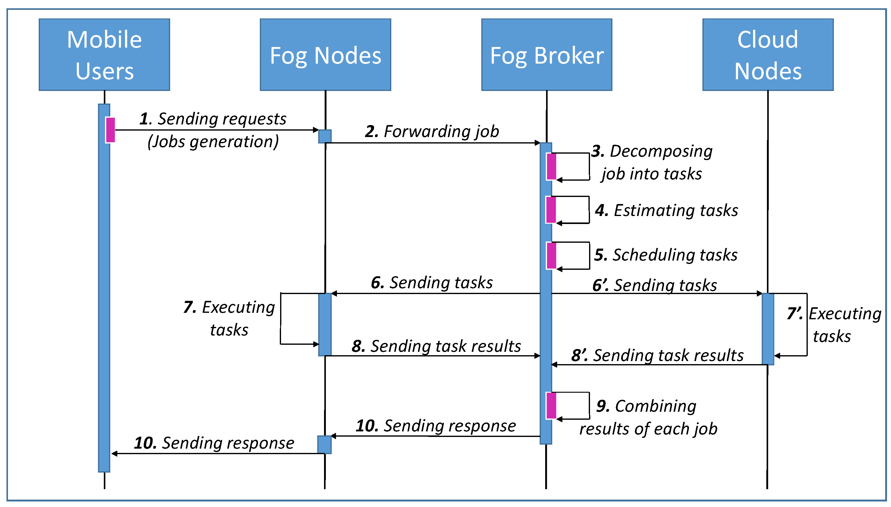
3.1. System Architecture

In the Fog environment, the processing takes place in a data hub on a smart device, or in a smart router, gateway, switcher, local server, etc. Because of limited processing capacity, some Fog nodes cooperate regionally together, simultaneously connecting to Cloud nodes known as Cloud virtual machines to satisfy mobile user’s need. It was assumed that our system consists of f Fog nodes and c Cloud nodes as well as a Fog broker. Fog nodes communicate directly to mobile users. All requests from mobile users are forwarded immediately to Fog broker, who is responsible for analyzing, estimating and then scheduling all tasks to be executed in the Cloud–Fog system. The Fog broker is close to the Fog nodes, thus the time consumed for data communication between each other is negligible.
To guarantee the performance of system, the TCaS algorithm, which is installed on the Fog broker, aims at finding an optimal task executing schedule achieving time and cost efficiency. The operation of our system model is described step by step in Figure 1.
Firstly, a mobile user sends a request (Step 1), which is handled by Fog node it is connected to. This request (or job) is immediately forwarded to the Fog broker (Step 2). To be processed in distributed system, each job is decomposed into a set of tasks (Step 3), and then the number of instructions and the resource usage needed are estimated (Step 4). Handling all information of tasks and nodes, the Fog broker runs a scheduling algorithm (Step 5) to find a good task assignment. Following the output, tasks are sent to the corresponding Cloud nodes and Fog nodes (Step 6). Each node is responsible for processing all tasks assigned (Step 7) and then sends the results back to the Fog broker(Step 8). Once all tasks are completed, the result of the job is combined (Step 9) by the Fog broker. Subsequently, the response is sent to the mobile user through the Fog node that user connects with (Step 10).

3.2. Problem Formulation

When requests from BoT applications are sent to the Fog layer, they are decomposed into small and independent tasks to be processed over the Cloud–Fog computing infrastructure. Each task has the following properties: number of instructions, memory required, size of input and output files. Assuming that T k indicates the kth task, at each time, there is a set of n independent tasks sent to the system, as follows:
T = T 1 , T 2 , T 3 , . . . , T n .
The Cloud–Fog computing infrastructure consists of processors, i.e., Cloud nodes and Fog nodes, which have the same attributes such as CPU rate, CPU usage fee, memory usage fee, and bandwidth usage fee. However, Cloud nodes are typically more powerful than the Fog nodes, but the cost of using them is greater. The set of m processors including c Cloud nodes and f Fog nodes in the system ( N = N c l o u d N F o g ) is expressed as:
N = N 1 , N 2 , N 3 , . . . , N m ,
where N i presents the ith processing node.
Each task T k ( T k T a s k s ) is assigned to the processor N i ( N i N o d e s ) , which is represented as T k i . One processor can be assigned to process a set of one or more tasks:
N i T a s k s = T x i , T y i , . . . , T z i
The task scheduling problem in Cloud–Fog computing environment could be formulated as searching of a set:
N o d e T a s k s = T 1 a , T 2 b , T 3 c , . . . , T n p
For a set of tasks N i T a s k s , the execution time ( E X T ) that node N i needs to complete all tasks assigned is:
E X T N i = T k i N i T a s k s E x e T i m e ( T k i ) = T k i N i T a s k s l e n g t h ( T k ) C P U r a t e ( N i )
where E x e T i m e ( T k i ) is the execution time of T k processed in node N i , which is calculated by:
E x e T i m e ( T k i ) = l e n g t h ( T k i ) C P U r a t e ( N i )
with l e n g t h ( T k ) the number of instructions of task T k and C P U r a t e ( N i ) the CPU rate of node N i , which is determined based on clock rate, number of cores, instruction level parallelism, etc.
M a k e s p a n is the total time for the system to complete all tasks, defined from the time when the request is received to the time that the last task is completed, or the time when the last machine finishes. M a k e s p a n is determined by the formula:
M a k e s p a n = M a x 1 i m E X T N i
Let M i n M a k e s p a n be the lower bound of M a k e s p a n , i.e., the shortest time that the system needs to complete all tasks. Ideally, when all nodes finish all tasks assigned at the same time, M i n M a k e s p a n will be obtained and calculated by:
M i n M a k e s p a n = E X T N 1 = . . . = E X T N m
thus,
M i n M a k e s p a n = 1 k n l e n g t h ( T k ) 1 i n C P U r a t e ( N i )
When one task is executed in Cloud–Fog system, a monetary amount must be paid for processing cost, memory usage cost, and bandwidth usage cost. The cost estimated when node N i processes the task T k is expressed as:
C o s t ( T i k ) = c p ( T i k ) + c m ( T i k ) + c b ( T i k )
In Equation (5), each cost is calculated as follows.
Processing cost is defined as:
c p ( T k i ) = c 1 E x e T i m e ( T k i )
where c 1 is the CPU usage cost per time unit in node N i , and E x e T i m e ( T k i ) is defined as Equation (6).
Letting c 2 be the memory usage cost per data unit in node N i and M e m ( T k ) the memory required by task T k , the memory usage cost is:
c m ( T k i ) = c 2 M e m ( T k i )
Task T k processed in node N i needs an amount of bandwidth B w ( T k ) , which is the sum of input and output file size. Let c 3 be the bandwidth usage cost per data unit; the bandwidth usage cost is defined as follows:
c b ( T k i ) = c 3 B w ( T k i )
Total cost for all tasks to be executed in Cloud–Fog system is calculated as follows:
T o t a l C o s t = T k i N o d e T a s k s C o s t ( T k i )
M i n T o t a l C o s t is the lowest cost needed for a set of tasks T to be completed in Cloud–Fog system, which can be obtained when each task is assigned to the cheapest node. Provided the information of each node, it is easy to determine which node processes task T k with the lowest cost, known as M i n C o s t ( T k ) . Therefore, M i n T o t a l C o s t is specific with one set of tasks T, and can be defined as:
M i n T o t a l C o s t = T k T M i n C o s t ( T k ) = T k T M i n 1 i m ( C o s t ( T k i ) )
We can define a utility function that computes the trade-off between the M a k e s p a n and total cost as follows:
F = α M i n M a k e s p a n M a k e s p a n + 1 α M i n T o t a l C o s t T o t a l C o s t
where α ( α [ 0 , 1 ] ) is the balance coefficient between makespan and total cost. α = 0.5 means that time and cost have same priority in optimizing. When α > 0.5 , our mechanism focuses on minimizing the makespan with higher priority than total cost, which is the case when a user is willing to pay more money to obtain better performance. Inversely, when α < 0.5 , the cost is more prioritized than time, i.e., the user has a tight budget.
The objective is optimizing execution time and processing cost, which means finding a solution such that M a k e s p a n and T o t a l C o s t are minimum and close to M i n M a k e s p a n and M i n T o t a l C o s t , respectively. Consequently, the closer to 1 the utility function F is, the more optimal is the solution obtained.
The task scheduling problem in Cloud–Fog computing environment can be formulated as:
Input:
T = T 1 , T 2 , T 3 , . . . , T n : a set of independent tasks
N = N 1 , N 2 , N 3 , . . . , N m : a set of processing nodes including Cloud nodes and Fog nodes
Output:
N o d e T a s k s = T 1 a , T 2 b , T 3 c , . . . , T n p : an assignment of all tasks executed into processing nodes
Objective:
Maximize the utility function F:
F = α M i n M a k e s p a n M a k e s p a n + 1 α M i n T o t a l C o s t T o t a l C o s t M a x

4. Evolutionary Algorithms for Task Scheduling Problem

4.1. Modified Particle Swarm Optimization

In [25], Izakian proposed Particle Swarm Optimization (PSO) for grid job scheduling. For the purpose of approaching task scheduling problem in Cloud–Fog computing environment with various evolutionary algorithms, we remove the service layer in grid computing and maintain the general idea of PSO to define Modified Particle Swarm Optimization (MPSO), which can adapt to our proposed model. Details of the MPSO algorithm are given in the following.

4.1.1. Particle: Position and Velocity

The representation step plays an important role in the successful design of PSO algorithm, which aims at finding an appropriate mapping between problem solution and PSO particle. In our method, binary representation is used, each particle is expressed as a m × n matrix, called position matrix, in which m is the number of available nodes including Fog nodes and Cloud nodes and n is the number of tasks. X k , which is the position matrix of tth particle in the swarm, has two main characteristics:
i.
X k ( i , j ) 0 , 1 ( i , j ) , i 1 , 2 , , m , j 1 , 2 , , n
ii.
i = 1 m X k ( i , j ) = 1 ( j ) , j 1 , 2 , , n
In position matrix, each element is either 0 or 1. If X k ( i , j ) = 1 , then task T j is executed in node N i . The second condition ensures that there is exactly one element with value 1 in each column, which means each task is performed on only one node.
For example, a set of 10 tasks is executed in a Cloud–Fog system of the nodes; one solution of task scheduling can be:
N o d e T a s k s = T 1 3 , T 2 1 , T 3 3 , T 4 2 , T 5 1 , T 6 2 , T 7 2 , T 8 3 , T 9 1 , T 10 3
An example of the position matrix of particle corresponding to the above solution is shown in Figure 2.
Each particle moves to a new position based on its velocity. The velocity matrix dimensions are exactly the same as the position matrix, i.e., m × n . Its elements are real numbers in the range V m a x , V m a x . In other words, the kth particle has velocity V k satisfying the condition:
V k ( i , j ) V m a x , V m a x ( i , j ) , i 1 , 2 , , m , j 1 , 2 , , n .

4.1.2. Population Initialization

Assuming that N particles form a population, first the position of each particle in the initial population is generated randomly, which ensures that particles are distributed in many areas in the search space. Besides, the velocity matrices of particles are initialized stochastically for the purpose of dynamic exploration.

4.1.3. Fitness Function

Particles are evaluated through a fitness function, the fitness value represents the quality of the solution that the particle expresses and also shows its influence in the population. In this problem, the fitness value is calculated by the utility function F shown in Equation (15). The higher is the fitness value, the better is the solution achieved.

4.1.4. Personal Best and Global Best

Through many movements, particles explore various locations. The personal best p B e s t k determines the best position that kth particle has experienced, whereas the global best g B e s t indicates the best place that any particle of the whole population has discovered from the beginning of the algorithm. Thus, p B e s t and g B e s t are m × n binary matrices as position matrices.
The two factors p B e s t and g B e s t play important roles in the process of PSO, which help each particle to search around its own best position and the global best position. p B e s t and g B e s t should be updated every time step. When the kth particle moves to new position X k , if a greater fitness value is achieved, its personal best p B e s t k is replaced with X k . If fitness value of any p B e s t is greater then current g B e s t , g B e s t is replaced with that p B e s t .

4.1.5. Particle Updating

The velocities of particles are updated regularly based on its best experience p B e s t and the leader g B e s t . The below equation indicates how kth particle updates its velocity.
V k ( t + 1 ) ( i , j ) = w . V k t ( i , j ) + c 1 r 1 ( p B e s t k t ( i , j ) X k t ( i , j ) ) + c 2 r 2 ( g B e s t k t ( i , j ) X k t ( i , j ) ) .
In Equation (16), each element in velocity matrix is updated. ( i , j ) indicates the element in ith rows and jth column of the matrix. c 1 snf c 2 are positive acceleration constants, which control the influence of p B e s t and g B e s t on the search process, r 1 and r 2 follow uniform distributions in the range of 0 , 1 , and w is inertia weight, which usually decreases from a large value (e.g., 0.9) in the beginning to a small value (e.g., 0.1) in the last iteration to control the exploration and exploitation abilities of the swarm.
The new position of kth particle is defined as follows.
X k ( t + 1 ) ( i , j ) = 1 , i f V k ( t + 1 ) ( i , j ) = m a x i V k ( t + 1 ) ( i , j ) , i 1 , 2 , , m ; 0 , o t h e r w i s e .
The new position of kth particle is updated based on its velocity. Equation (17) means that, in each column of position matrix, the element whose corresponding element in velocity matrix has the max value in its column is assigned a value of 1, while others in this column are labeled 0. If a column of velocity matrix has many elements with max value, then one will be selected randomly and 1 assigned to its corresponding element of position matrix.

4.2. Proposed Evolutionary Algorithm

To deal with task scheduling problem in Cloud–Fog computing environment, the TCaS algorithm is proposed based on an evolutionary algorithm—Genetic Algorithm (GA)—as follows.

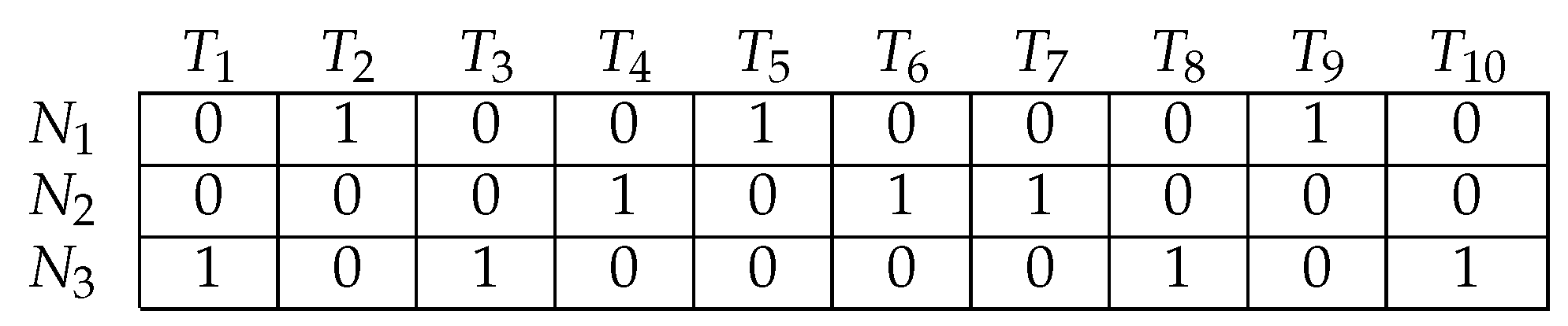
4.2.1. Encoding of Chromosomes

An individual specified by a chromosome in genetic algorithm represents a solution of task scheduling. For encoding of chromosomes, an n-dimensional array corresponding to n genes is used. The sequence number of gene is the sequence number of task; each gene has a value of an integer k in range [ 1 ; m ] with m the number of nodes, which indicates that the corresponding task is assigned to the node numbered k.
For the example shown in Section 4.1.1, the c h r o m o s o m e expresses that solution would be:
c h r o m o s o m e = 3 , 1 , 3 , 2 , 1 , 2 , 2 , 3 , 1 , 3
Node 1 executes the set of tasks 2 , 5 , 9 , the set of tasks 4 , 6 , 7 is assigned to be processed in node 2, while node 3 is responsible for the set of tasks 1 , 3 , 8 , 10
This chromosome encoding method was chosen because of the flexibility of performing genetic operations, such as crossover and mutation, to create new individuals exploring the solution search space, simultaneously inheriting quality gene segments from parents. The order of tasks processed is not considered because performing tasks in a different order on one machine does not affect the objectives, namely makespan and total cost.

4.2.2. Population Initialization

The initial population is the set of all individuals that are used in the GA to find the optimal solution. Assume that the size of population is N . To discover many areas in the search space as well as to ensure the diversity of the population in the first generation, the N individuals are initialized randomly. From the initial population, the individuals are selected, and some operations are applied on them to form the next generation.

4.2.3. Fitness Function

The fitness function is the measure of the superiority of an individual in the population. The individual with high fitness value represents a good quality solution. The fitness value of each individual is estimated by the utility function F shown in Equation (15). Depending on the fitness value, the individuals can survive or die out through each generation.

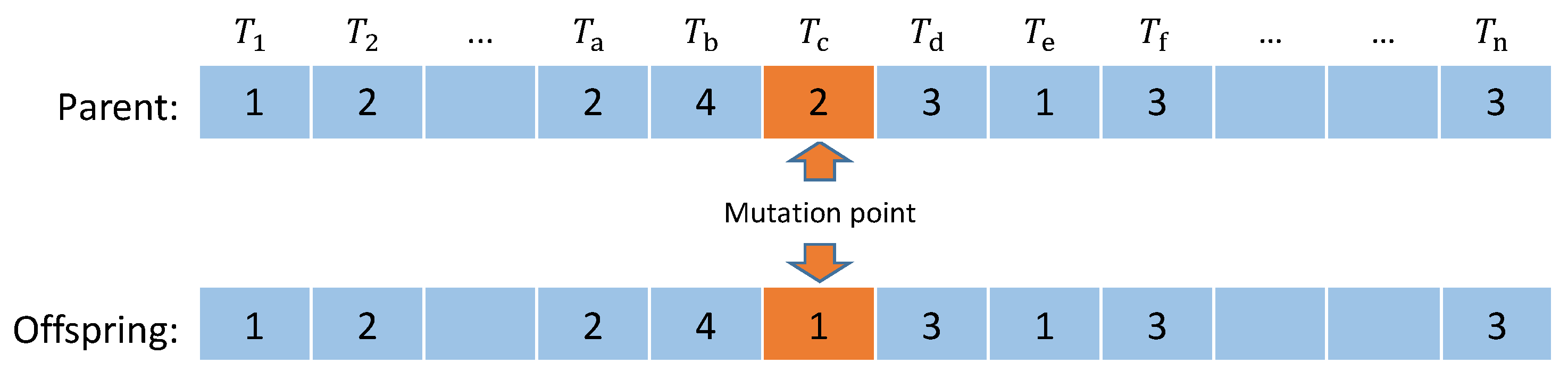
4.2.4. Genetic Operators

a. Crossover operator
With chromosome encoding as an array of integers, two-point crossover operation is used to generate offspring inheriting good genes from parents. This operation is shown in Figure 3, where two crossover points are randomly selected, the first parent exchanges the middle gene segment to the second parent, and the remaining genes are unchanged, forming a new individual.
In the crossover process over the population, parental selection influences the efficiency of the algorithm. Each individual has a crossover rate of α . Everyone in the population is considered to be the first parent with the probability α , and then the roulette wheel technique is applied to select the second parent in the population to participate in crossover process. With this selection technique, high quality individuals with a larger fitness value have higher probability of being selected as parent, thus ensuring good gene segments are more likely preserved in the next generation.
b. Selection strategy
The selection mechanism is used to select individuals to form a population for the next generation based on the Darwin’s law of survival. Immediately after the crossover process, natural selection is conducted. The offspring is calculated for the fitness value and is compared to the parent; if the offspring is better than the parent, the individual is preserved to form the next-generation population. Otherwise, this offspring is discarded and the parent is retained in the next generation.
This greedy selection maintains the diversity of the population over generations when the genes of the lesser individuals are not eliminated so rapidly and still contribute to the exploration of new regions on the search area; simultaneously, good gene segments are not repeated too many times in individuals in one population.
c. Mutation operator
After crossover and natural selection process, new population is formed with N individuals. Each individual participates in one-point mutation with the rate of γ . The location of the mutant gene is randomly selected and replaced by a different value (see Figure 4); in this way, the task chosen is assigned to be processed in another node.
Mutation perfects the limitations of crossover operator by finding the optimal solution when individuals are vicious around the extremes, or escaping from the local extremes to explore the other areas in the solution space.
According to the proposed TCaS algorithm, a set of modifications from GA was introduced. These modifications are as follows.
  • Parental selection: In the crossover process, each individual in the population is considered to be the first parent, and the second parent was selected by the roulette wheel technique.
  • Greedy selection strategy: Each crossover operation produces one offspring, which is preserved to form the next-generation population if it is better than first parent and discarded otherwise.

5. Performance Evaluation

In this section, we present the simulation setup and evaluation of the proposed algorithm based on the results of conducted tests.

5.1. Experimental Settings

Cloud and Fog nodes have different processing power as well as resource usage cost. We assumed that each node has its own processing capacity represented by processing rate (measured by MIPS (million instructions per second)), along with CPU, memory and bandwidth usage cost. Thirteen processing nodes constructed the Cloud–Fog system, with the characteristics shown in Table 3. In the Fog layer, Fog nodes such as routers, gateways, workstations, or personal computers have limited processing capacity. In Cloud layer, servers or virtual machines in high performance data centers are responsible for handling tasks. Therefore, the processing speed of Cloud nodes is much faster than Fog nodes. In contrast, the cost of using resources in the Cloud is more expensive than in the Fog. These costs are calculated according to Grid Dollars (G$)—a currency unit used in the simulation to substitute for real money.
The Cloud–Fog system is responsible for executing all requests from users. Each request is decomposed into a set of tasks, which are analyzed and the resources that they need are estimated. It was assumed that each tack has some attributes: number of instructions, memory required, input file size, and output file size. Depending on the workload of each request, the set of tasks may vary widely in size. Thus, 11 datasets with from 40 to 500 tasks were created to participate in our simulation. Each task in datasets was generated randomly with its attributes following Table 4. With randomness, the experiment could cover various scenarios because many types of tasks were created, some of them requiring a huge amount of processing while others needing more memory or bandwidth usage, and so on. Note that we proposed these benchmarks (e.g., Table 3 and Table 4) because of no benchmarks published in the literature in this research area.
The settings of the experimental environment are shown in Table 5, the simulation was developed in Java with Eclipse editor, and using iFogSim [26]. iFogSim Was chosen because it is developed based on CloudSim, a Cloud computing platform that has been widely used and validated in numerous studies over the years; iFogSim supports modeling and simulation of architecture as well as services in Cloud–Fog environment.
Since our proposed TCaS algorithm is based on Genetic Algorithm, we compared our method with some other evolutionary algorithms: (1) Modified Particle Swarm Optimization (MPSO); and (2) Bee Life Algorithm (BLA) [4]; as well as a traditional algorithm: (3) simple Round Robin (RR) scheduling. BLA was introduced by Bitam with the following idea.
BLA is an optimization method that is inspired from the two most important behaviors of bees, namely marriage (or reproduction) and food foraging. First, N individuals, which form the initial population, are evaluated by a fitness function. After sorting the population, the best individual is chosen as the queen, the next D bees are identified as drones, and the remaining bees W are workers bee. Population is changed through each generation; the bee’s life cycle consists of two main behaviors: reproduction and food foraging. During the reproduction stage, the queen mates with a set of drones to produce broods by the crossover and mutation operators. The individual evaluation is conducted to find the best bee who substitutes the precedent queen, the following D fittest bees become drones and W new workers. Now, the food foraging stage is executed; each worker is responsible for finding the food source and then recruiting other workers to collect the found food. Afterwards, the best worker of every region keeps alive in the next population.
Table 6 shows the parameter settings of three evolutionary algorithms.
In Equation (15), the balance coefficient α indicates the priority of optimization between makespan and total cost. We first conducted simulations in the scenario where time and cost have the same level of interest, i.e., α = 0.5 .

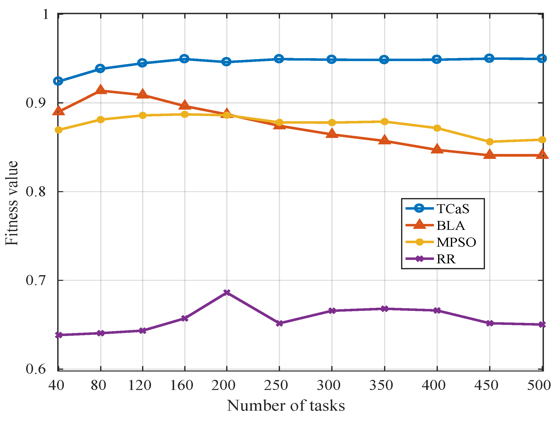
5.2. Experimental Results

To analyze our method, several experiments were conducted in two different scenarios. In the first situation, a bag of tasks was executed locally in a set of connected Fog nodes and, in the other, Fog layer collaborated with a number of Cloud nodes to process requests from users.

5.2.1. Scenario 1: Task Scheduling in Fog Environment

In the first setup, we defined a Fog layer consisting of 10 Fog nodes, which connected to each other to satisfy user requirements in a geographical area. Four algorithms were deployed to produce schedules for bags of tasks, which included from 40 to 500 tasks to be executed in Fog environment. The average results were obtained by running four algorithms in each dataset over 30 times with 500 generations (or iterations) and the coefficient balance α = 0.5 .
Figure 5 shows the comparison of time–cost trade-off of four algorithms. It was obvious that our proposed algorithm, TCaS, dominated the first position in every dataset with high average fitness value of 0.945, which was better than MPSO, BLA and RR by one average 7.97%, 8.17% and 44.08%, respectively. Experiencing on small datasets, from 40 to 200, BLA gave better solutions than MPSO. However, when the dataset was bigger, i.e., the problem became more complex, the fitness value BLA reached recorded a gradual decrease with the increase in dataset size; meanwhile, MPSO maintained its stability with its fitness value of around 0.87. Consequently, MPSO algorithm produced better solutions than BLA by an average of 1.89% on datasets with size from 250 to 500. The simple RR algorithm gave the worse results of the three algorithms with fitness value of around 0.65.
Table 7 presents the scheduling length and processing cost of the four algorithms. The fitness function was contributed by two main components: makespan and total costs. Thus, with high fitness value, TCaS algorithm demonstrated superiority on almost datasets in both time and cost aspects. Our proposed method overtook all other algorithms in execution time; the schedule of TCaS algorithm consumed less time than that of MPSO by 16.15% and BLA by 16.77%, and saved on average 2.32 times over the whole 11 datasets compared to that of RR algorithm. Considering the monetary cost, TCaS required the least cost of the four algorithms on almost all datasets, except on the smallest dataset of 40, where BLA won. TCaS saved 0.48%, 0.53% and 2.15% of processing cost compared to BLA, MPSO and RR algorithm, respectively.

5.2.2. Scenario 2: Task Scheduling in Cloud–Fog Environment

In this case, we conducted experiments on the complete Cloud–Fog system, which consisted of 10 Fog nodes and three remote Cloud nodes. Unlike in Scenario 1, Fog nodes had similar values of attributes; tasks seemed to be evenly distributed to nodes. In this case, the processing nodes were divided into two categories. Cloud nodes were much more powerful than Fog nodes, thus were responsible for processing more tasks. Therefore, finding an optimal solution was more difficult.
Figure 6 compares the time–cost trade-off between our proposed TCaS algorithm and the three others as the number of tasks changed. The average results were obtained by running two algorithms on each dataset over 30 times with 500 generations (or iterations) and the coefficient balance α = 0.5 . Compared to Scenario 1, the ranking of solution quality of the four algorithms achieved in this case were quite similar; however, the fitness values were generally smaller. TCaS algorithm still overwhelmed the remaining algorithms on all datasets, especially on small datasets including from 40 to 200 tasks. The result achieved by TCaS was on average better than that of MPSO by 11.04%, BLA by 15.11% and RR by 44.17%. Observing three evolutionary algorithms, the fitness value slightly decreased as the number of tasks increased. This can be explained as the bigger the dataset was, the larger search the space was, thus the three algorithms could not converge in the limited iterations or could not explore the whole large space with a small number of individuals. MPSO performed better than BLA in this complex environment, while achieving higher fitness value than BLA on every datasets and was better than BLA on average by 3.66%. The fitness value RR algorithm achieved remained the lowest level of four algorithms, which was around 0.55.
Table 8 compares the four algorithms in terms of execution time and processing cost. TCaS algorithm represented the superiority of scheduling length on every dataset; it saved on average 35.73% of processing time compared to MPSO, 42.20% compared to BLA and 176.25% compared to RR. However, in terms of monetary cost, our algorithm was not the best. MPSO demonstrated its cost effectiveness when holding the first position on almost all datasets except the 40-task dataset where BLA was slightly better. TCaS consumed 5.96% more money than MPSO, the most cost effective algorithm; however, this number is very small compared to the execution time benefit shown by TCaS. Actually, response time is very important in guaranteeing QoS as it directly affects a user’s experience, thus users are willing to spend a small amount of money to experience much higher performance service.
Based on the analysis of the results of the two scenarios, TCaS, our proposed algorithm, could reach better trade-off between makespan and total cost than the three other algorithms, together with showing the superiority of time optimization. MPSO demonstrated more power than BLA in complex environments. RR algorithm with simple mechanism gave poor results.
Next, we considered the convergence of the three evolutionary algorithms TCaS, BLA and MPSO. They were performed on a dataset of 120 tasks over 500 generations with coefficient balance α = 0.5 . We observed the population every 20 generations. The fitness values of all individuals were synthesized, as shown in Figure 7. The middle point in line indicates the average fitness value of whole population while the bottom and top of the error bar present the fitness value of the worst and best individual, respectively. It was observed that BLA and MPSO expressed fast convergences after 100 generations, however, the found solutions had small fitness values at 0.69 and 0.72 compared with 0.84 achieved by TCaS algorithm. In some first generations, individuals of TCaS algorithm were distributed with a wide range of fitness value. The best solution was found in 240th generation; afterwards, the fitness range narrowed, meaning the population gathered around the extreme. TCaS converged after 300 generations. The mechanism of BLA that all drones perform crossover operator with only one queen each generation made the population easily fall into local extreme. Similarly, in MPSO, the leader had a great influence on every particle in the population, thus there was high probability that the population fell into local extreme when the leader was stuck. Consequently, both algorithms converged quickly with low fitness values. Meanwhile, the proposed TCaS algorithm maintained population diversity, thus could reach more optimal solution.
Figure 8 indicates the effect of balance coefficient α in time and cost achieved by TCaS algorithm when a set of 120 tasks was processed. In the case α = 0 , monetary cost was maximized, however makespan was too large at 1827 s because many tasks were assigned centrally to cheap nodes. When α = 0.5 , makespan was improved 5.09 times while 1.20 times of total cost was needed compared with case α = 0 . Increasing α gradually to 1, the scheduling length decreased slightly together with a small amount of cost added. This is because execution time was more concentrated to be optimized than cost. This experiment showed that, by adjusting the balance coefficient α , our model could flexibly satisfy user’s requirements when they are interested in high performance execution or cost efficiency.

6. Conclusions and Future Work

In this work, we focused on task scheduling problem for BoT applications in Cloud–Fog computing environment. The TCaS algorithm based on an evolutionary algorithm was proposed and it performance evaluated in various scenarios. TCaS outperformed three other methods, namely MPSO, BLA, RR, in both Fog environment and Cloud–Fog system. In Cloud–Fog system, it was better on average than MPSO by 11 . 04 % , BLA by 15.11% and RR by 44.17% over 11 sets of tasks in terms of trade-off between time and cost execution, especially obtaining much shorter scheduling length. Moreover, the proposed algorithm could flexibly satisfy user’s requirement of high performance processing or cost efficiency.
In the future, we will research, improve, and apply more algorithms to solve scheduling problem, especially evolutionary algorithms. In addition, we plan to expand scheduling problem by focusing on optimizing many other goals, such as time, transmission costs, computing resources, and energy consumption to satisfy users. Constraints of budget, deadline, and resource limitation can be added for greater practicality.

Author Contributions

Software, T.T.A.; Writing—Original Draft Preparation, T.T.A. and D.B.S.; Writing—Review and Editing, H.T.T.B. and B.M.N.; and Project Administration, B.M.N and H.T.T.B.

Acknowledgments

This research is funded by the Hanoi University of Science and Technology (HUST) under project number T2018-PC-017.

Conflicts of Interest

The authors declare no conflict of interest.

References

  1. Fog Computing and the Internet of Things: Extend the Cloud to Where the Things Are. Cisco White Paper. 2015. Available online: https://www.cisco.com/c/dam/en_us/solutions/trends/iot/docs/computing-overview.pdf (accessed on 25 November 2018).
  2. Stiles, J.R.; Bartol, T.M.; Salpeter, E.E.; Salpeter, M.M. Monte Carlo Simulation of Neuro- Transmitter Release Using MCell, a General Simulator of Cellular Physiological Processes. In Computational Neuroscience; Bower, J.M., Ed.; Springer: Boston, MA, USA, 1998. [Google Scholar]
  3. Smallen, S.; Casanova, H.; Berman, F. Applying Scheduling and Tuning to On-line Parallel Tomography. In Proceedings of the Proceedings of the 2001 ACM/IEEE conference on Supercomputing, Denver, CO, USA, 10–16 November 2001. [Google Scholar]
  4. Bitam, S.; Zeadally, S.; Mellouk, A. Fog computing job scheduling optimization based on bees swarm. Enterp. Inf. Syst. 2017, 12, 373–397. [Google Scholar] [CrossRef]
  5. Peter, N. Fog computing and its real time applications. Int. J. Emerg. Technol. Adv. Eng. 2015, 5, 266–269. [Google Scholar]
  6. Chiang, M.; Zhang, T. Fog and IoT: An overview of research opportunities. IEEE Internet Things J. 2016, 3, 854–864. [Google Scholar] [CrossRef]
  7. Shi, Y.; Ding, G.; Wang, H.; Roman, H.E.; Lu, S. The fog computing service for healthcare. In Proceedings of the 2015 2nd International Symposium on Future Information and Communication Technologies for Ubiquitous HealthCare (Ubi-HealthTech), IEEE, Beijing, China, 28–30 May 2015; pp. 1–5. [Google Scholar]
  8. Yi, S.; Li, C.; Li, Q. A survey of fog computing: Concepts, applications and issues. In Proceedings of the 2015 Workshop on Mobile Big Data, Santa Clara, CA, USA, 29 October–1 November 2015; pp. 37–42. [Google Scholar]
  9. Suárez-Albela, M.; Fernández-Caramés, T.; Fraga-Lamas, P.; Castedo, L. A practical evaluation of a high-security energy-efficient gateway for IoT fog computing applications. Sensors 2017, 17, 1978. [Google Scholar] [CrossRef] [PubMed]
  10. Bonomi, F.; Milito, R.; Natarajan, P.; Zhu, J. Fog computing: A platform for internet of things and analytics. In Big Data and Internet of Things: A Roadmap for Smart Environments; Springer: Berlin, Germany, 2014; pp. 169–186. [Google Scholar]
  11. Yousefpour, A.; Ishigaki, G.; Jue, J.P. Fog computing: Towards minimizing delay in the internet of things. In Proceedings of the 2017 IEEE International Conference on Edge Computing (EDGE), Honolulu, HI, USA, 25–30 June 2017; pp. 17–24. [Google Scholar]
  12. Lee, K.; Kim, D.; Ha, D.; Rajput, U.; Oh, H. On security and privacy issues of fog computing supported Internet of Things environment. In Proceedings of the 2015 6th International Conference on the Network of the Future (NOF), Montreal, QC, Canada, 30 September–2 October 2015; pp. 1–3. [Google Scholar]
  13. Hong, K.; Lillethun, D.; Ramachandran, U.; Ottenwälder, B.; Koldehofe, B. Mobile fog: A programming model for large-scale applications on the internet of things. In Proceedings of the Second ACM SIGCOMM Workshop on Mobile Cloud Computing, Hong Kong, China, 16 August 2013; pp. 15–20. [Google Scholar]
  14. Mahmud, R.; Kotagiri, R.; Buyya, R. Fog computing: A taxonomy, survey and future directions. In Internet of Everything; Springer: Singapore, 2018; pp. 103–130. [Google Scholar]
  15. Binh, H.T.T.; Anh, T.T.; Son, D.B.; Duc, P.A.; Nguyen, B.M. An Evolutionary Algorithm for Solving Task Scheduling Problem in Cloud–Fog Computing Environment. In Proceedings of the SOICT 9th Symposium on Information and Communication Technology, Da Nang City, Vietnam, 6–7 December 2018; pp. 397–404. [Google Scholar]
  16. Gu, L.; Zeng, D.; Guo, S.; Barnawi, A.; Xiang, Y. Cost efficient resource management in fog computing supported medical cyber-physical system. IEEE Trans. Emerg. Top. Comput. 2017, 5, 108–119. [Google Scholar] [CrossRef]
  17. Deng, R.; Lu, R.; Lai, C.; Luan, T.H.; Liang, H. Optimal workload allocation in fog-cloud computing toward balanced delay and power consumption. IEEE Internet Things J. 2016, 3, 1171–1181. [Google Scholar] [CrossRef]
  18. Guo, X.; Singh, R.; Zhao, T.; Niu, Z. An index based task assignment policy for achieving optimal power-delay tradeoff in edge cloud systems. In Proceedings of the 2016 IEEE International Conference on Communications (ICC), Kuala Lumpur, Malaysia, 23–27 May 2016; pp. 1–7. [Google Scholar]
  19. Ningning, S.; Chao, G.; Xingshuo, A.; Qiang, Z. Fog computing dynamic load balancing mechanism based on graph repartitioning. China Commun. 2016, 13, 156–164. [Google Scholar] [CrossRef]
  20. Oueis, J.; Strinati, E.C.; Barbarossa, S. The fog balancing: Load distribution for small cell cloud computing. In Proceedings of the 2015 IEEE 81st Vehicular Technology Conference (VTC Spring), Glasgow, UK, 11–14 May 2015; pp. 1–6. [Google Scholar]
  21. Abdi, S.; Motamedi, S.A.; Sharifian, S. Task scheduling using modified PSO algorithm in cloud computing environment. In Proceedings of the International Conference on Machine Learning, Electrical and Mechanical Engineering, Dubai, UAE, 8–9 January 2014; pp. 8–9. [Google Scholar]
  22. He, J.; Cheng, P.; Shi, L.; Chen, J.; Sun, Y. Time synchronization in WSNs: A maximum-value-based consensus approach. IEEE Trans. Autom. Control 2014, 59, 660–675. [Google Scholar] [CrossRef]
  23. Li, D.; Sun, X. Nonlinear Integer Programming; Springer Science & Business Media: Berlin, Germany, 2006; Volume 84. [Google Scholar]
  24. Kuhn, H.W. The Hungarian method for the assignment problem. Naval Res. Logist. (NRL) 2005, 52, 7–21. [Google Scholar] [CrossRef] [Green Version]
  25. Izakian, H.; Tork Ladani, B.; ZamanifarAjith, A. A Novel Particle Swarm Optimization Approach for Grid Job Scheduling; Springer: Berlin/Heidelberg, Germany, 2009; Volume 31, pp. 100–109. [Google Scholar]
  26. Gupta, H.; Dastjerdi, A.V.; Ghosh, S.K.; Buyya, R. iFogSim: A Toolkit for Modeling and Simulation of Resource Management Techniques in Internet of Things. Edge Fog Comput. Environ. 2017, 47, 1275–1296. [Google Scholar]
Figure 1. The operation of Cloud–Fog system.
Applsci 09 01730 g001
Figure 2. Example of the position matrix.
Applsci 09 01730 g002
Figure 3. Two-point crossover operator.
Applsci 09 01730 g003
Figure 4. One-point mutation operator.
Applsci 09 01730 g004
Figure 5. Time–cost trade-off comparison of the four algorithms.
Applsci 09 01730 g005
Figure 6. Time–cost trade-off comparison of the four algorithms.
Applsci 09 01730 g006
Figure 7. Convergence comparison between three evolutionary algorithms.
Applsci 09 01730 g007
Figure 8. Time and cost as the balance coefficient α changes.
Applsci 09 01730 g008
Table 1. Comparison between Cloud computing and Fog computing.
ParameterCloud ComputingFog Computing
LatencyHighLow
Response time of the systemLowHigh
ArchitectureCentralizedDistributed
Communication with devicesFrom a distance via Internet, Multiple hopsDirectly from the edge via Various protocols and standards, One hop
Data processingFar from the source of information in long-term timeClose to the source of information in short-term time
Computing capabilitiesHigher (Cloud Computing does not provide any reduction in data while sending or transforming data)Lower (Fog Computing reduces the amount of data sent to Cloud computing.)
Server nodesFew nodes with scalable storage and computing powerVery large nodes with limited storage and computing power
SecurityLess secure, UndefinedMore secure, Can be defined
Working environmentWarehouse-size building with air conditioning systemsOutdoor (e.g., Streets, gardens) or indoor (e.g., Restaurants)
Location of server nodesWithin the InternetAt the edge of the local network
Table 2. Summary of related works about task scheduling algorithms for Fog computing.
ArticleIdeasImprovement CriteriaLimitation
Huynh Thi Thanh Binh (2018) [15]genetic algorithmexecution time, processing costsmall dataset
Bitam et al. (2017) [4]bee life algorithmexecution time, memorysmall dataset, only in Fog environment
Gu et al. (2017) [16]two-phase linear programming-based heuristiccommunication cost, apply for cellular networkno computational offloading capability
Deng et al. (2016) [17]nonlinear integers, Hungarian methodpower consumption, delaysuitable for centralized infrastructure, not easy to apply to Fog computing
Guo et al. (2016) [18]Markov decision problemspower consumption, delaya continuous-time queueing system
Ningning et al. (2016) [19]graph partitioning, a minimum spanning treeexecution timecomplexity when the number of user requests increases
Queis et al. (2015) [20]heuristicuser satisfaction, task latency, power consumptioncomplexity when the number of user requests increases
Abdi et al. (2014) [21]particle swarm optimizationcompletion of taskin Cloud environment
Table 3. Characteristics of the Cloud–Fog infrastructure.
ParameterFog EnvironmentCloud EnvironmentUnit
Number of nodes103node
CPU rate 500 , 1500 3000 , 5000 MIPS
CPU usage cost 0.1 , 0.4 0.7 , 1.0 G$/s
Memory usage cost 0.01 , 0.03 0.02 , 0.05 G$/MB
Bandwidth usage cost 0.01 , 0.02 0.05 , 0.1 G$/MB
Table 4. Attributes of tasks.
PropertyValueUnit
Number of instructions 1 , 100 10 9 instructions
Memory required 50 , 200 MB
Input file size 10 , 100 MB
Output file size 10 , 100 MB
Table 5. Simulation setup.
SystemIntel® Core T M i7-4710MQ, CPU 2.50GHz
Memory8 GB
SimulatoriFogSim
Operating systemWindows 10 Professional
Table 6. BLA, TCaS and MPSO parameters.
ParameterBLATCaSMPSO
Running times303030
queen1
drones ( D ) 30
Population size ( N )workers ( W ) 69100100
Crossover rate ( α ) 90%90% c 1 = c 2 = 1.5
Mutation rate ( γ ) 1%1% w = 0.9 0.1
Number of generations500500500
Table 7. Makespan and total cost comparison of the four algorithms.
Number of TasksMakespan (s)Total Cost (G$)
TCaSBLAMPSORRTCaSBLAMPSORR
40191.44*207.57215.27456.11733.85730.88740.38755.98
80394.69416.09445.35963.081540.231540.851553.431581.82
120607.71654.92686.201495.662363.372367.592381.162418.90
160819.97917.67932.331912.083176.173183.803197.013246.69
200940.871067.491065.941905.703755.213767.373778.273835.40
2501,270.961490.651479.843054.804988.945017.175007.595079.06
3001,473.791765.491712.763309.145832.695877.415862.525935.94
3501,649.042010.741911.273638.196607.526653.376632.386738.19
4001,944.582421.982300.514347.647738.567816.047759.957875.39
4502,235.162840.792751.295350.358845.908926.578876.309016.59
5002,503.093174.393067.266023.749902.649995.979921.7610,097.75
* The bold indicates the superiority of the corresponding algorithm throughout four algorithms.
Table 8. Makespan and total cost comparison of the four algorithms.
Number of TasksMakespan (s)Total Cost (G$)
TCaSBLAMPSORRTCaSBLAMPSORR
40114.37*185.37157.41313.01861.53811.34811.45859.96
80232.91368.78352.50965.321817.901732.461689.261793.53
120357.42580.29546.701267.542779.722639.792583.552687.34
160515.38776.68763.411729.193694.693543.083464.333587.65
200633.28894.42873.061521.444403.634247.694134.094323.92
250816.591127.481112.332190.215485.855349.455155.445411.28
3001052.921436.581375.542861.956740.366591.756405.116666.58
3501241.281628.911583.822835.657666.277535.36751.257610.78
4001486.921925.291864.293139.768877.148763.91882.878792.12
4501754.182251.062168.703653.4610,124.5610,033.839682.4510,026.13
5001994.212512.402425.864633.4811,299.5311,219.1810,823.8411,266.31
* The bold indicates the superiority of the corresponding algorithm throughout four algorithms.

