Numerical Analysis of the Mechanical Behaviors of Various Jointed Rocks under Uniaxial Tension Loading


State Key Laboratory of Mining Disaster Prevention and Control, Shandong University of Science and Technology, Qingdao 266590, China
*
Author to whom correspondence should be addressed.
Appl. Sci. 2019, 9(9), 1824; https://doi.org/10.3390/app9091824
Submission received: 1 April 2019
/
Revised: 23 April 2019
/
Accepted: 27 April 2019
/
Published: 1 May 2019
(This article belongs to the Special Issue Fatigue and Fracture of Non-metallic Materials and Structures)
Abstract
:In a complex stress field of underground mining or geotechnical practice, tension damage/failure in rock masses is easily triggered and dominant. Unlike metals, rocks are generally bi-modularity materials with different mechanical properties (Young’s modulus, etc.) in compression and tension. It is well established that the Young’s modulus of a rock mass is directly related to the presence of the fracture or joint, and the Young’s modulus estimation for jointed rocks and rock masses is essential for stability analysis. In this paper, the tensile properties in joint rocks were investigated by using numerical simulations based on the discrete element method. Four influencing parameters relating to the tensile properties (joint dip angle, joint spacing, joint intersection angle, and joint density) were studied. The numerical results show that there is an approximately linear relationship between the joint dip angle (α) and the joint intersection angle (β) with the tensile strength (σt), however, the changes in α and β have less influence on the Young’s modulus in tension (Et). With respect to joint spacing, the simulations show that the effects of joint spacing on σt and Et are negligible. In relation to the joint density, the numerical results reveal that the joint intensity of rock mass has great effect on Et but insignificant effect on σt.
1. Introduction
For brittle materials such as rock, tension failure is one of the most significant failure modes [1]. In a complex stress field of underground mining or geotechnical practice, tension damage/failure in rock masses is easily triggered and dominant because: (1) The tensile strength (σt) of rocks is much lower than their compressive strength, and (2) joints and fractures of rock mass can offer little resistance to tensile stress [2]. After an excavation is taken underground, tension failure and its induced fractures will occur in surrounding rock masses near the opening [3,4,5,6,7,8]. The initiated fractures will develop/propagate and bring weakening effects on the rock masses under the effect of time and constant stress disturbance (development of entry or shaft, mining activities, etc.). As it is well established that the Young’s modulus of a rock mass is directly related to the fracture or joint intensity [9,10,11,12,13], the aforementioned fracture development can be described as a Young’s modulus degradation process in the view of an equivalent material method in continuum mechanics.
The macroscopic mechanical behaviors of intact and jointed rocks have been widely investigated, most of which has been focused on the material behaviors in compression [14,15,16]. However, unlike metals or other materials, rocks are generally bi-modularity materials with different Young’s moduli and Poisson’s ratios in compression and tension. Previous studies done by direct tension tests showed that the Young’s modulus in tension (Et) was always no larger than the compressive Young’s modulus (Ec) [17,18,19,20,21]. Hawkes et al. [17] conducted direct tension tests on different kinds of rocks, and the results showed that the ratio of Et/Ec was 1/9 for Barre sandstone and 0.5 for Barre granite. Stimpson and Chen [20] acquired the ratios to be 0.5, 1.0, 0.7, and 0.3–0.4 for four different rocks from cyclic loading uniaxial tension and compression tests. Similar results were obtained by Yu et al. [22] with an originally developed loading frame for direct tension. It has been addressed by researchers that the improper assumption that Et equals to Ec may lead to errors in calculating stress distributions around underground openings by means of analytical or numerical analysis, as well as in determining the tensile strength of rocks with Brazilian tests [18,20,22,23].
To date, it is still quite challenging to conduct direct uniaxial tension tests on intact rock specimens in laboratories due to the difficulties in avoiding: 1) Unfavorable stress concentration over the grip and 2) bending moments due to the non-coaxial gripping and curvature of the specimen. Various attempts have been made in this regard. Stimpson and Chen [20] conducted their tests on rock samples with a special hollow cylinder geometry. Okubo and Fukui [24] glued the rock samples directly to the loading platen to carry out direct tension tests. Fahimifar and Malekpour [25] developed a direct tension apparatus with hard steel tension jaws to ensure the connection between samples and the apparatus and that the applied load is pure tension. Fuenkajorn and Klanphumeesri [26] developed a compression-to-tension load converter to determine the tensile strength and Young’s modulus from dog-bone-shaped specimens.
As described above, the Young’s modulus estimation for jointed rocks and rock masses is essential for stability analysis. However, rock specimens with joints or fractures are difficult to be prepared, and simplifications have to be made with rock-like materials (such as gypsum) or simple notches. Furthermore, the uniaxial tension tests rely on specially made, non-universal apparatuses.
In recent years, numerical and computational resources have taken significant leaps forward, and numerical methods have become strong and efficient research tools by overcoming the limitations in laboratory and physical tests. Some previous studies have been done with numerical modelling on the direct tension testing of rock specimens. Tang et al. [1] studied the growth of micro-fractures in a specimen under uniaxial tension and the influence of heterogeneity on rock strength with a self-developed finite element code (RFPA2D). Wang et al. [27] simulated crack initiation, propagation, and coalescence for intact, single-notched, and double-notched rock specimens with RFPA3D under uniaxial tension, and the effects of the separation distance and overlapping distance of the two notches were investigated. Hamdi et al. [28] studied the model I fracture propagation in brittle rock under direct tension by means of a discrete element method. Guo et al. [29] investigated fracture patterns in layered rocks under direct tension with a discrete element method.
According to the previous studies [1,27,28,29,30,31,32], the numerical studies on rock specimens under uniaxial or direct tension loads mainly focus on fracture initiation and propagation within the specimens. However, the effects on the mechanical behaviors of strength and deformability, i.e., tensile strength and Young’s modulus in tension, of jointed rock specimens subjected to uniaxial tension load are barely discussed. In this study, rock specimens with various joint conditions are modeled with 3DEC (a 3-Dimension Distinct Element Code by Itasca) due to its capability in simulating the behaviors of joints (slip, separation, deformation, etc.) under mechanical loading, and the effects of joints on the tensile properties are studied by means of uniaxial tension numerical tests. Tests of rock samples with single joint, and multiple joints with different joint geometry parameters are designed, and their effects on the tensile properties of rock specimens are investigated. The goal of this study is to understand the effects of joints on the tensile properties of rocks.
2. Numerical Modelling
The numerical model is constructed by means of 3DEC, which is a three-dimensional numerical program employing the distinct element method for discontinuum modelling. In the following analysis, rock specimen models with different joint conditions (single, multiple parallel, and intersecting joints) are built, and the effects of joints on the tensile properties are investigated by applying a uniaxial tension load. The specimen model is a cylinder with 50 mm in diameter and 100 mm in height, as suggested by the International Society of Rock Mechanics (ISRM) [33]. All joints are considered to cut through the specimen. A constant rate of 0.005 mm/step is applied to the upper and lower boundary to simulate the uniaxial tension load. After the specimens fail in tension, 1000 extra steps are calculated to capture the after-peak behavior. With the obtained stress–strain curves, σt and Et under different joint conditions are calculated, and the effects of joint condition on the tensile strength (σt) and Et are hereby investigated.
In 3DEC, joints or fractures are considered as elements with mechanical properties. The rock and joint properties [34] (listed in Table 1 and Table 2) are applied according to a study on tunnel stability analysis of an underground mine using 3DEC.
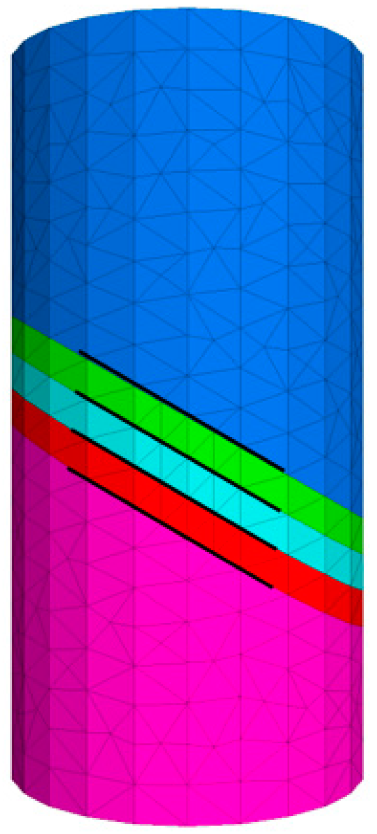
To study the effects of joints on the tensile properties of rocks, the rock specimens with various joint conditions were described and modelled with four geometry parameters of joints: α (the angle between the joint and the horizontal direction), d (the perpendicular distance between the two joints), β (the angle at which the two joints intersect), and n (the joint density).
In cases of rock specimens with two joints, the effects of the perpendicular distance between the two joints (d), the angle between the joint and the horizontal direction (α) of parallel joints, and the joint density (n) on the complete stress–strain response were studied by numerical simulation. When d was kept constant at 10, 20, 30, and 40 mm, four different homogeneity indexes (α) were considered, which were 20, 30, 40 and 50°, respectively. Similarly, when α were kept constant, d was varied as 10, 20, 30, and 40 mm. Moreover, when d and α were kept constant, n was changed from 2 to 6.
In cases of rock specimens with multiple joints, the effects of the perpendicular distance between the two cracks (d), the angle at which the two joints intersected (β), and the joint density (n) of intersecting joints on the complete stress–strain response were studied by numerical simulation. When d and n were kept constant as 0 mm and 2, there were six different homogeneity indexes (β) of 20, 40, 60, 80, and 100°. When β and n were kept constant, d was varied as 10, 20, 30, and 40mm. As a comparison, when d and n were kept constant, β was separately varied as 40, 60, 80, and 100°. When d and β were kept constant, n was changed from 4 to 12.
3. Effects of Joints on the Tensile Properties
3.1. Effect of the Dip Angle of A Single Joint
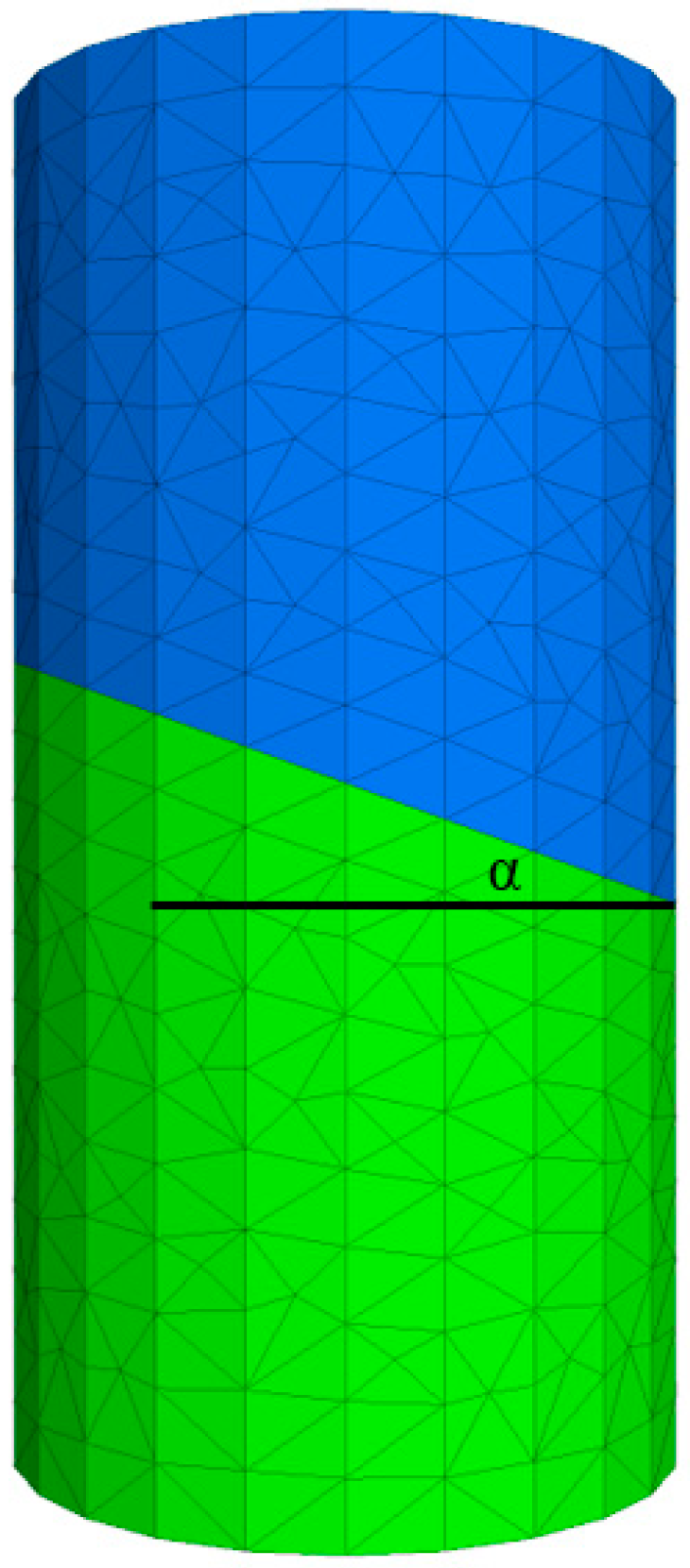
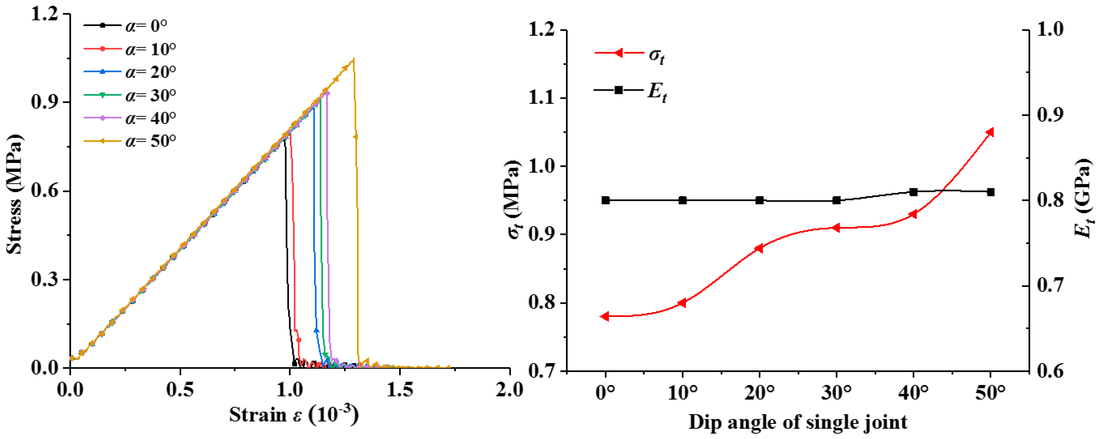
In this study, all joints are assumed to cut through the specimen. Seven models with different dip angles (α = 0, 10, 20, 30, 40, and 50°) were built, as illustrated in Figure 1. The stress–strain curves and the tensile properties with respect to dip angles are shown in Figure 2 and Table 3, respectively.
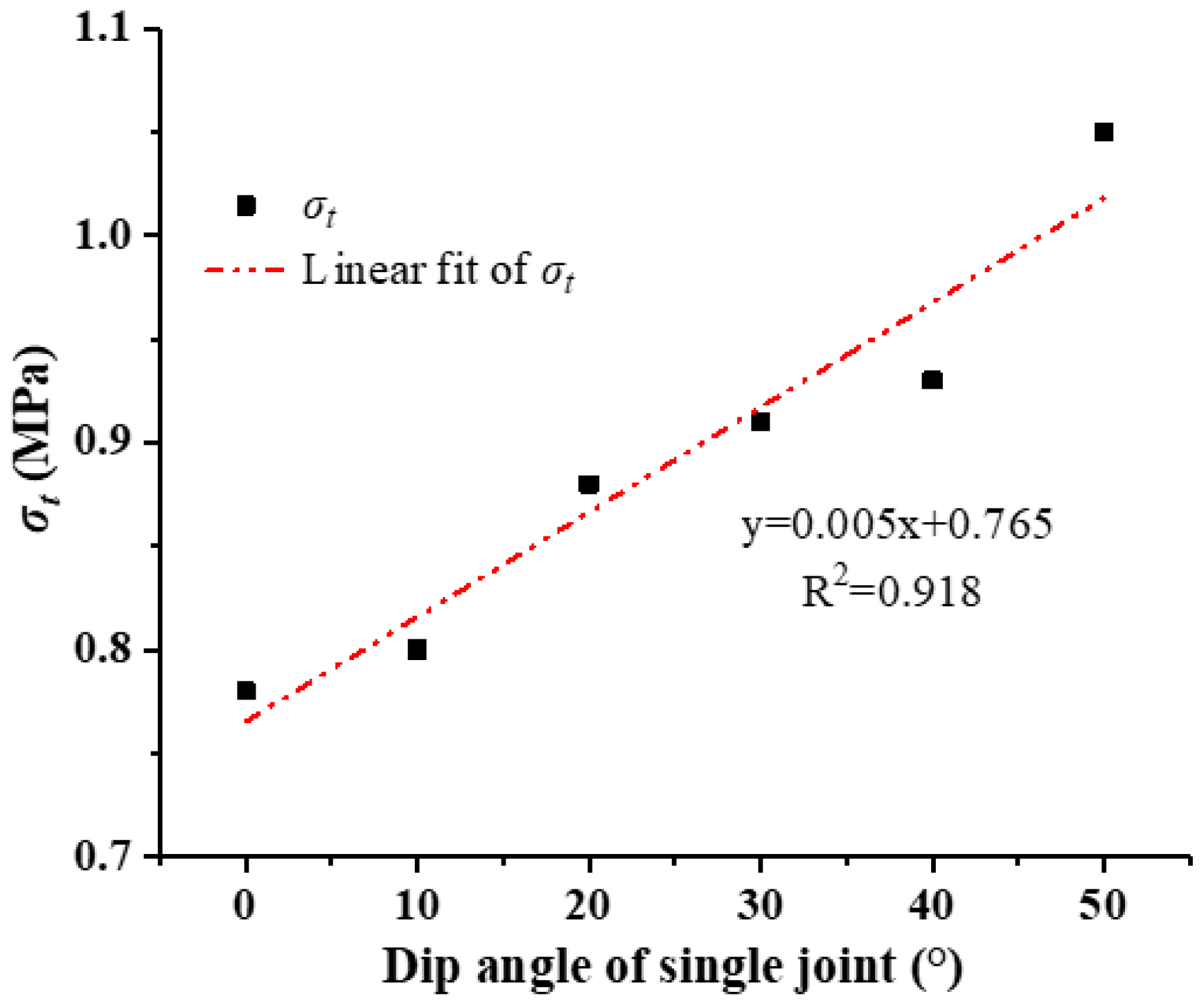
As can be seen, the general shapes of the stress–strain curves are similar. The stresses of specimens linearly increase after the tension loading starts, and undergo a sudden drop after failure, due to the brittle nature of rocks. The dip angle of the joint clearly has a notable effect on the tensile properties of the rock specimens. The peaks (σt) of the pre-peak curves vary monotonically increases with the increase of α.
When α = 0°, i.e., a horizontal joint, the σt and Et of the specimen are 0.78 MPa and 0.80 GPa, respectively. When α reaches 50°, the σt and Et increase to 1.05 MPa and 0.81 GPa, which are approximately 1.35 and 1.01 times the values in the case of α = 0°, respectively. In comparison, the changes in α have a greater influence on σt than Et. In reality, joint surfaces are usually rough, and the asperities provide resistance to shear stress, and the joint roughness is positively correlated to the shear strength [35]. The joint roughness is described with normal stiffness, shear stiffness, cohesion, etc. in 3DEC. When α is not 0°, the shear strength of the joint will provide extra resistance to the tensile load on rock failure and deformability, which leads to the high σt and Et when is α higher. However, when α = 0°, the joint is perpendicular to the tensile load, so no extra resistance can be provided from the shear behavior of the joint.
3.2. Effects of Parallel Joints on the Tensile Properties
Due to the existence of weak planes in rocks or rock masses, joints are the initiation points of rock and rock mass failure in most cases. Rock masses with multiple joints are common in engineering practice.
3.2.1. Effects of Joint Spacing and Dip Angle of Two Parallel Joints
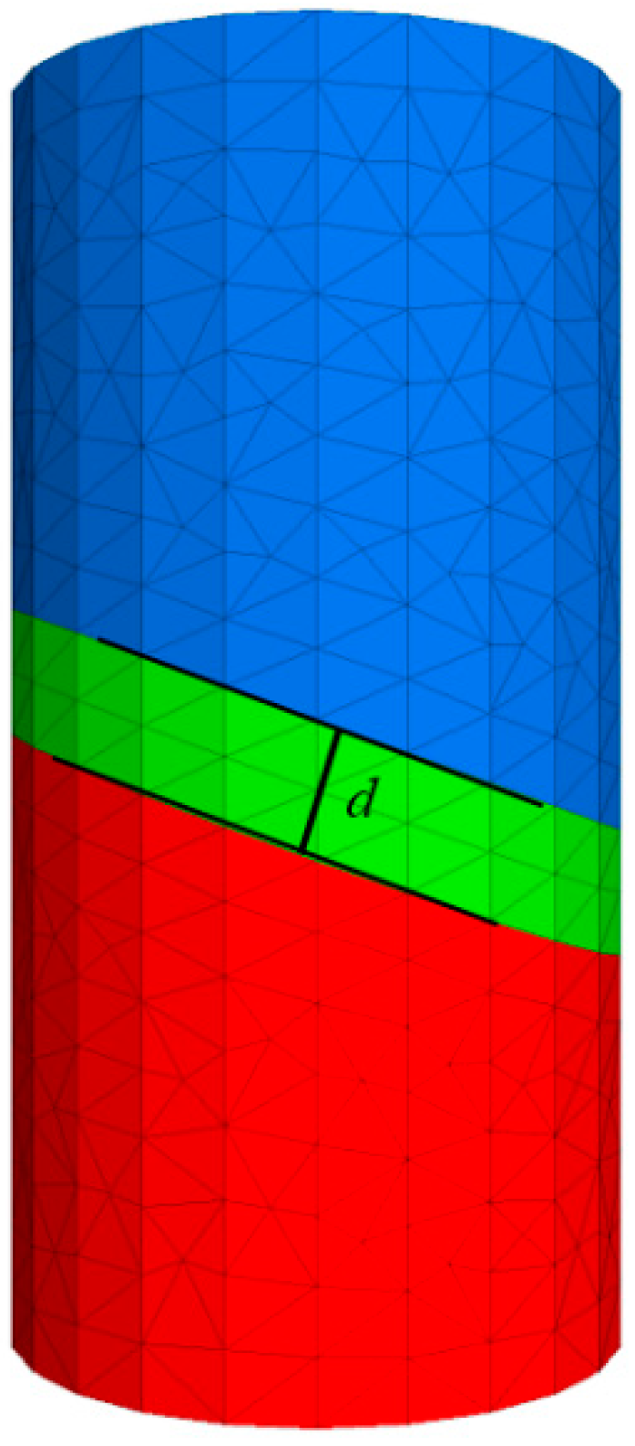
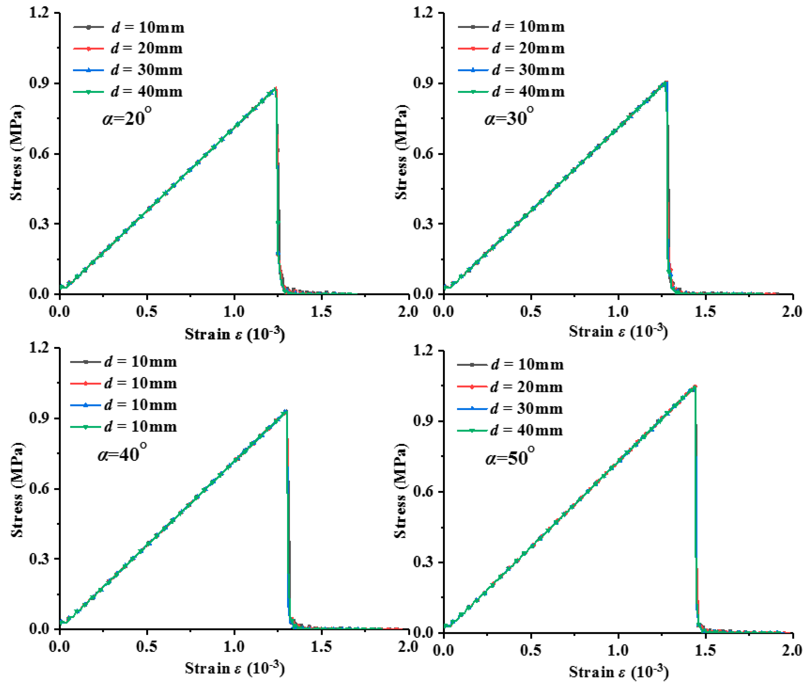
Joint spacing is the perpendicular distance between adjacent joints, and usually determines the sizes of the blocks making up the rock mass [2]. To investigate the effects of joint spacing (d) and dip angle (α) of two parallel joints on σt and Et, four sets of models with different dip angles (α = 20, 30, 40, and 50°) were built (as illustrated in Figure 4) under the condition of n = 2, and for each set of the model, four subsets with different joint spacing (d = 10, 20, 30, and 40 mm) were analyzed. The test program specifics are shown in Table 4, and the stress–strain curves under uniaxial tensile load are shown in Figure 5. The results are shown in Table 5.
As can be seen, the slopes and peaks of the curves, with same dip angle but different joint spacing, are almost the same, which means that the effect of joint spacing on σt and Et are negligible. When d decreases from 40 to 10 mm, σt and Et merely decrease by 0.003 MPa and 0.002 GPa, respectively. This result is obtained under the premise that no joint development is considered. In practice, joints will develop, and adjacent joints will connect and merge under mechanical loading. However, this study focuses on the effects of existing joints on the tensile properties. Similar to the results from Section 3.1, σt and Et are affected by the dip angle of the two parallel joints, but the effects vary. The dip angle has a greater effect on σt than Et. As the dip angle increases from 20 to 50°, σt increases from 0.88 to 1.05 MPa, while Et lightly increases from 0.71 to 0.73 GPa. When comparing with Table 3, it can be noticed that the value of σt is identical in the cases of single-jointed and double-jointed models with the same dip angle.
3.2.2. Effect of Joint Density of Parallel Joints
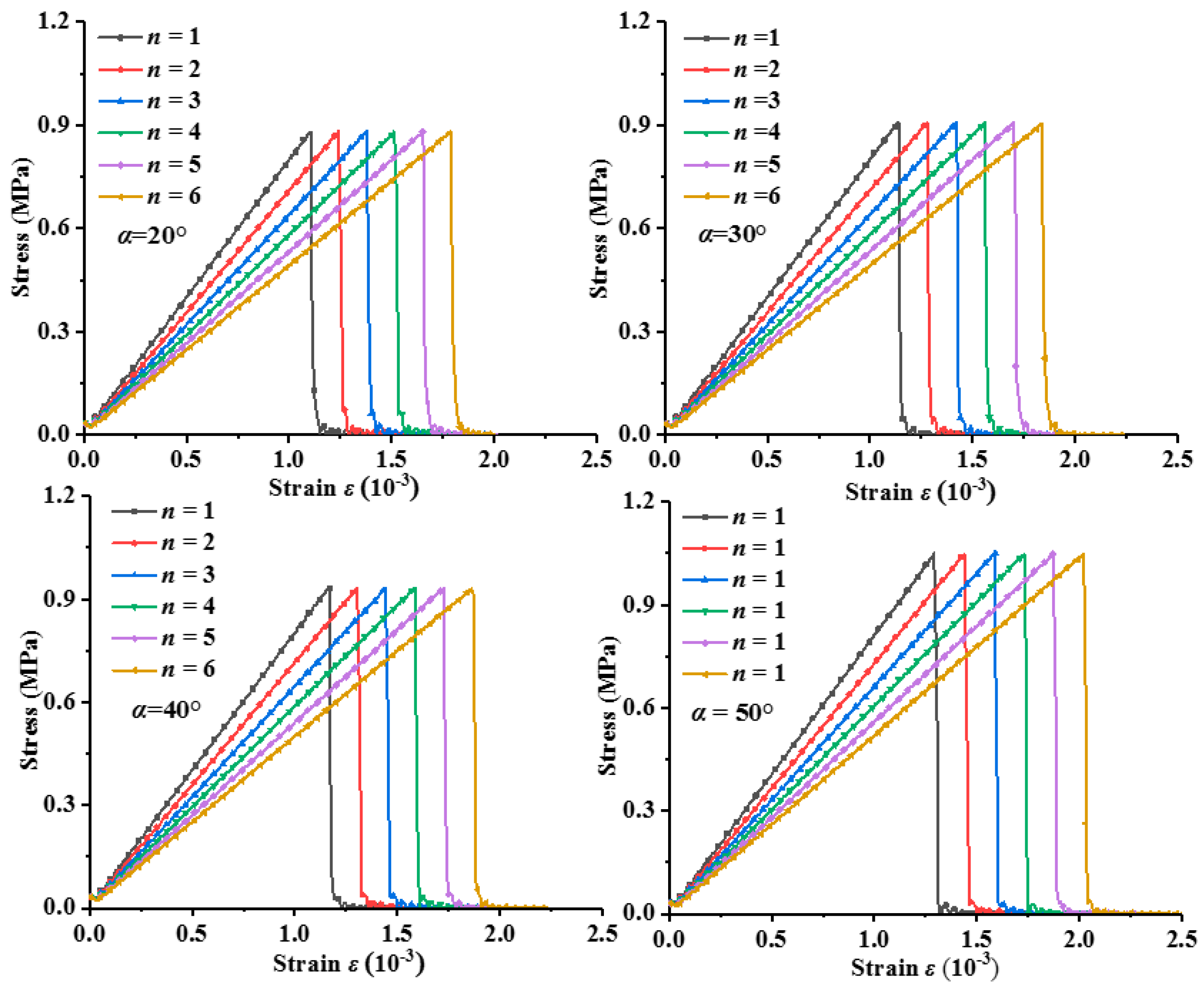
In a certain unit of rock mass, the number of joints is often referred to as the fracture intensity [36,37]. It is well addressed that the mechanism of deformation and failure of rock masses varies with fracture intensity, as well as the engineering properties such as cavability, permeability, and fragmentation characteristics. In this study, the effect of joint intensity on σt and Et is investigated by means of the number of joints (n) inside the specimen. Four sets of models with different dip angles (α = 20, 30, 40, 50°) were built (as illustrated in Figure 6) under the condition of d = 5 mm, and for each set of the model, six subsets with different numbers of joints (n = 1, 2, 3, 4, 5, 6) were analyzed. The test program specifics are shown in Table 6 and the stress–strain curves under uniaxial tensile load are shown in Figure 7. The results are shown in Table 7.
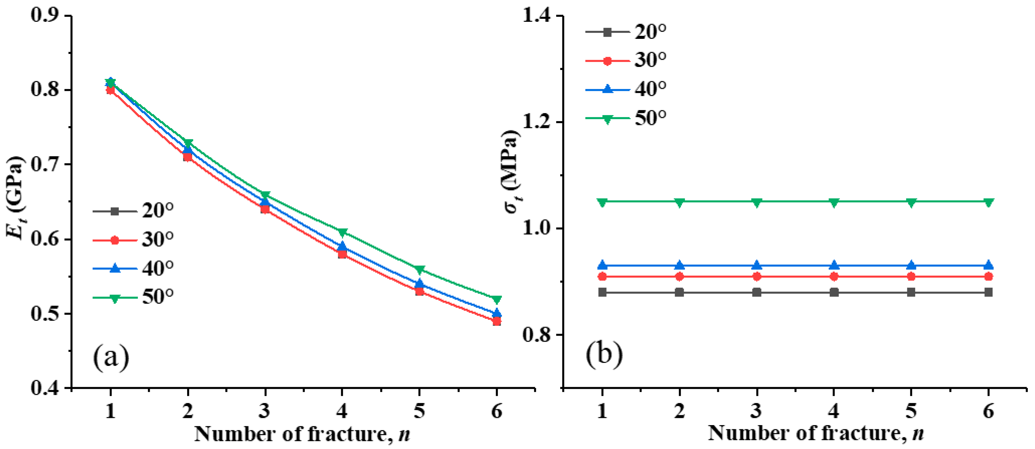
As can be seen, for each subset with the same α, the peaks of the curves are almost identical, while the slopes are notably effected by n. Taking the model set with α = 40° as an example, as listed in Figure 7, when n increases from 1 to 6, Et significantly drops from 0.81 to 0.52 GPa, while σt remains constant. The influencing pattern of n on Et is identical for different values of α. These results indicate that the fracture intensity of a rock mass has a great effect on Et but a negligible effect on σt.
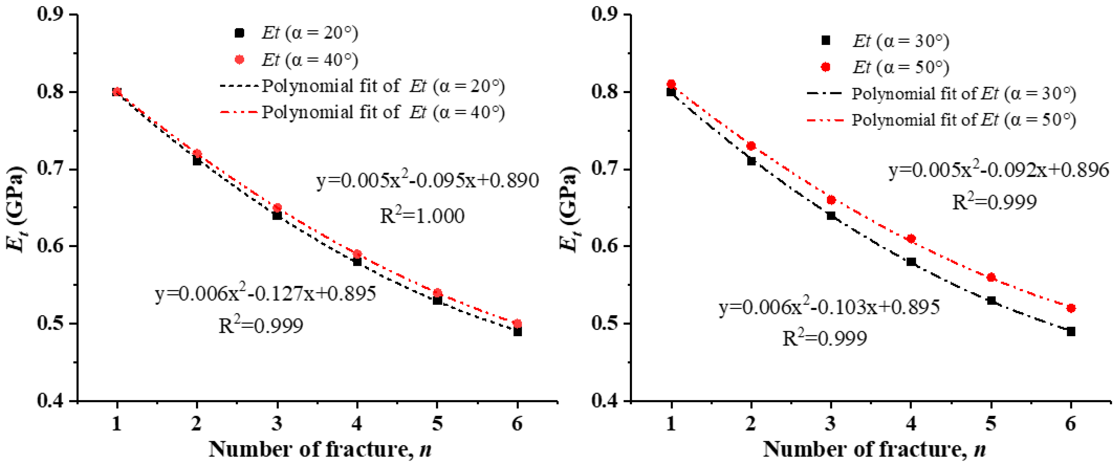
The relationship between n and Et with different values of α after fitting is shown in Figure 8. As can be seen, Et is negatively correlated to n, and the relationship varies with different values of α. The change in Et with n will be less significant in cases of higher values of α.
3.3. Effects of Intersecting Joints on the Tensile Properties
In actual rock engineering activities, the existence of fractures is usually very complicated. One or more intersecting joint sets, usually referred to as a joint system, are common in heavily jointed rock masses. In this section, the effects of intersecting joints on the tensile properties of rock specimens are analyzed.
3.3.1. Effect of the Intersection Angle of an Intersecting Joints Set
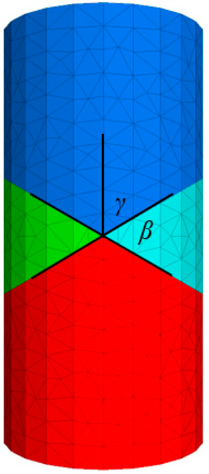
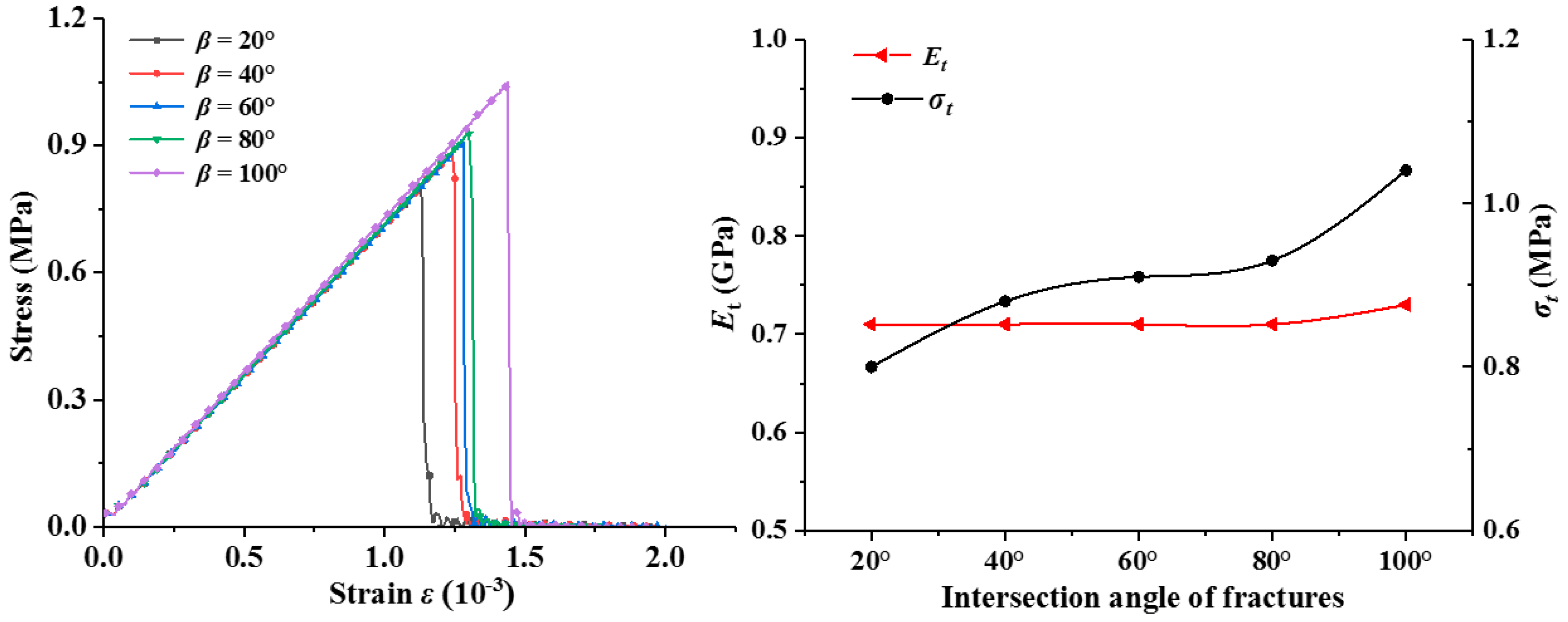
Seven models with symmetric intersecting joints, which have different intersection angles (β = 20, 40, 60, 80 and 100°), were built, as illustrated in Figure 9. The stress–strain curves and the tensile properties with respect to intersection angles are shown in Figure 10 and Table 8, respectively.
As can be seen, the general patterns of the stress–strain curves are analogous. The stresses of specimens linearly increase after the tension loading starts, and undergo a sudden drop after failure, exhibiting the brittle behavior of rocks. The intersection angle of the joint clearly has a remarkable effect on the tensile properties of the rock specimens. The peaks (σt) and the slopes (Et) of the pre-peak curves vary and t monotonically increase with the increase of β.
When β = 20°, the σt and Et of the specimen are 0.80 MPa and 0.71 GPa, respectively. When β reaches 100°, the σt and Et increase to 1.05 MPa and 0.73 GPa, which are approximately 1.3 and 1.03 times the values in the case of β = 20°, respectively. In contrast, the changes in β have a greater influence on σt than Et.
3.3.2. Effects of Joint Spacing and Intersection Angle of a Joints Set
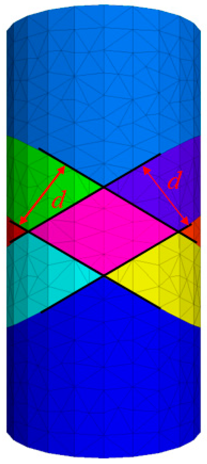
To investigate the effects of joint spacing (d) and intersection angle (β) of two intersection joints on σt and Et, four sets of models with different dip angels (β = 20, 40, 60, and 100°) were built (as illustrated in Figure 12), and for each set of the model, four subsets with different joint spacing (d = 10, 20, 30, and 40 mm) were analyzed. The test program specifics are shown in Table 9. The stress–strain curves under uniaxial tensile load are shown in Figure 13 and the results are shown in Table 10.
As can be seen, the slopes and peaks of the curves with same intersection angle but different joint spacing are almost the same, which means that the effects of joint spacing on σt and Et are trivial. When d increases from 10 to 40 mm, σt and Et merely increase by 0.0004 MPa and 0.0008 GPa, respectively. Similar to the results from Section 3.3.1, σt and Et are affected by the joint spacing of the intersection joints, but the effect varies. The intersection angle has a greater effect on σt than Et. As the intersection angle increases from 40 to 100°, σt doubles from 0.88 to 1.05 MPa, while Et lightly increases from 0.58 to 0.61 GPa. It can be noticed that the value of σt is identical in the cases of single-jointed and double-jointed models with identical β.
3.3.3. Effect of Joint Density of Intersection Joints
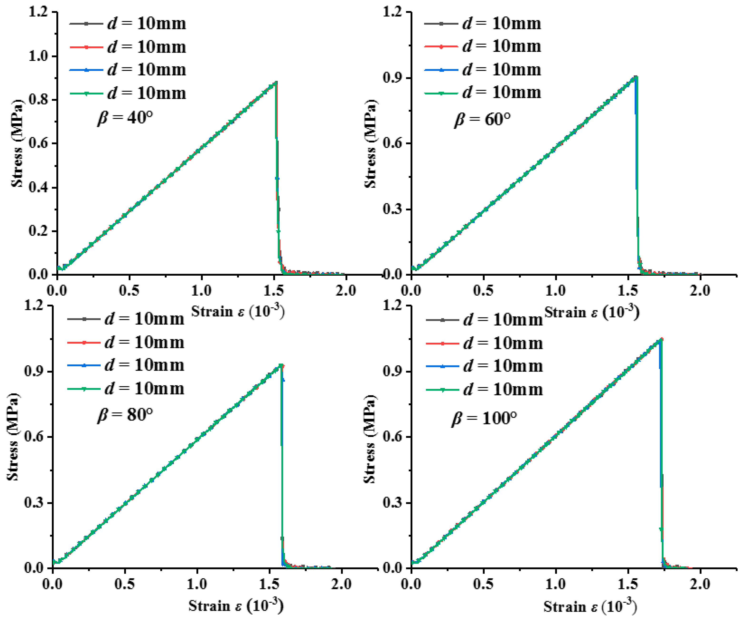
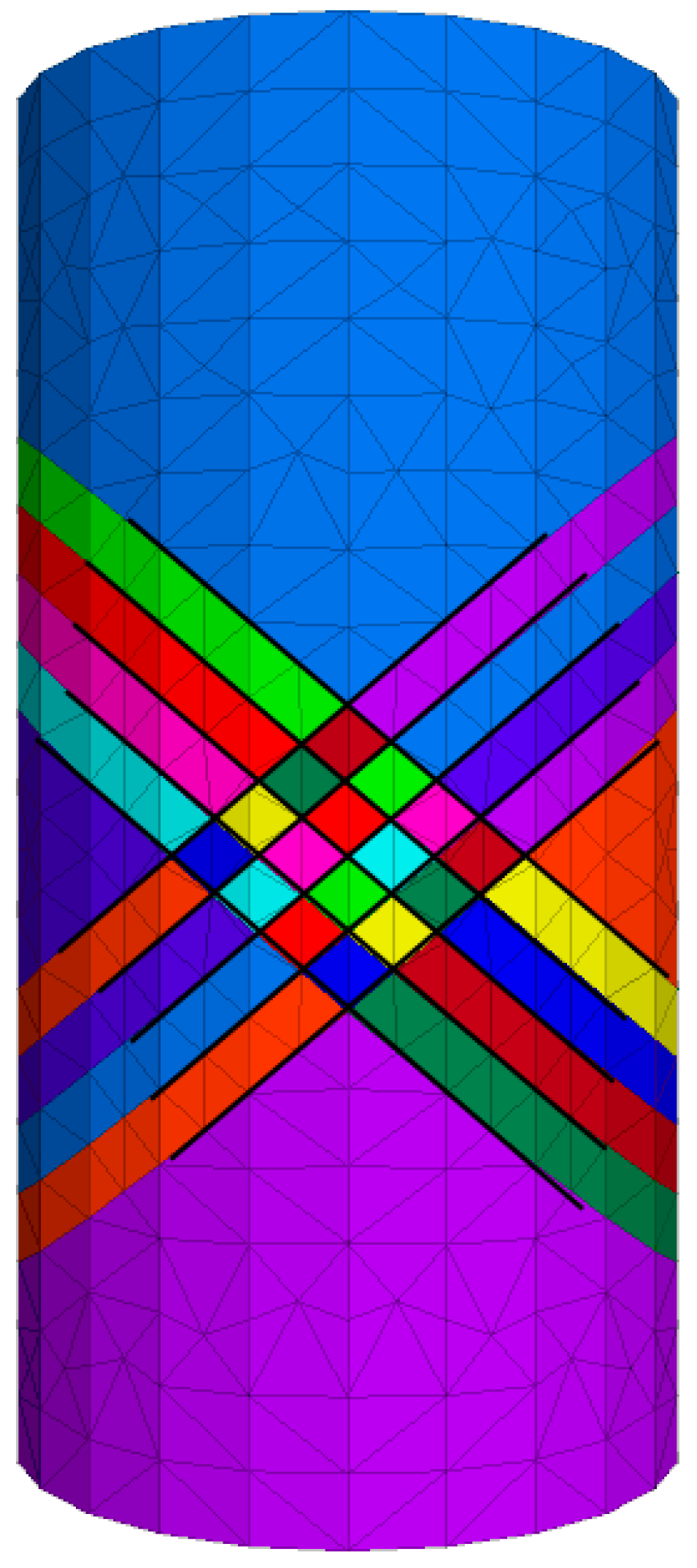
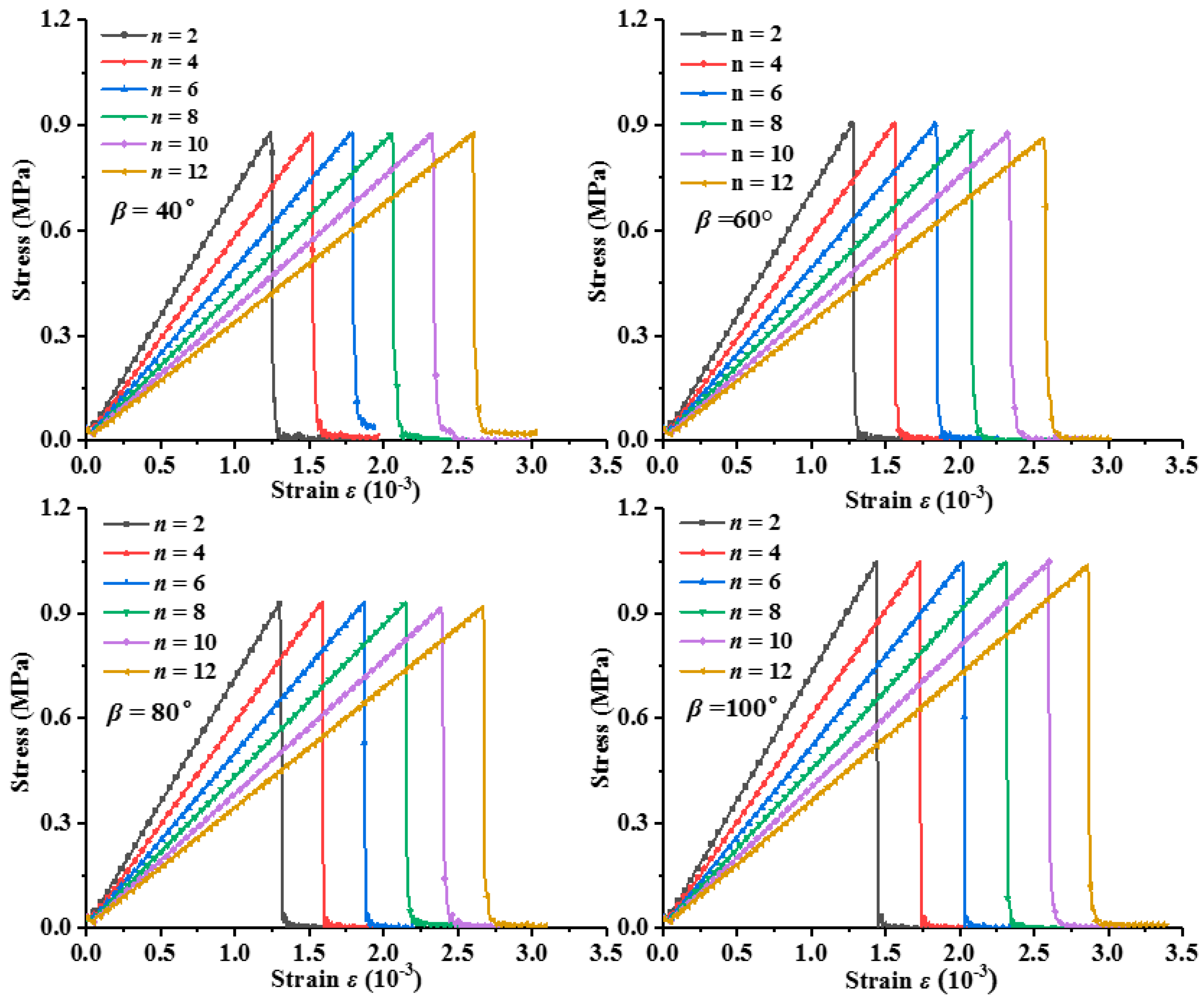
In this study, the effects of joint intensity on σt and Et are investigated by means of the number of joints (n) inside the specimen. Four sets of models with different dip angles (β = 40, 60, 80, and 100°) were built (as illustrated in Figure 14) under the condition of d = 5 mm, and for each set of the model, six subsets with different numbers of joints (n = 4, 6, 8, 10, and 12) were analyzed. The test program specifics are shown in Table 11 and the stress–strain curves under uniaxial tensile load are shown in Figure 15. The results are shown in Table 12
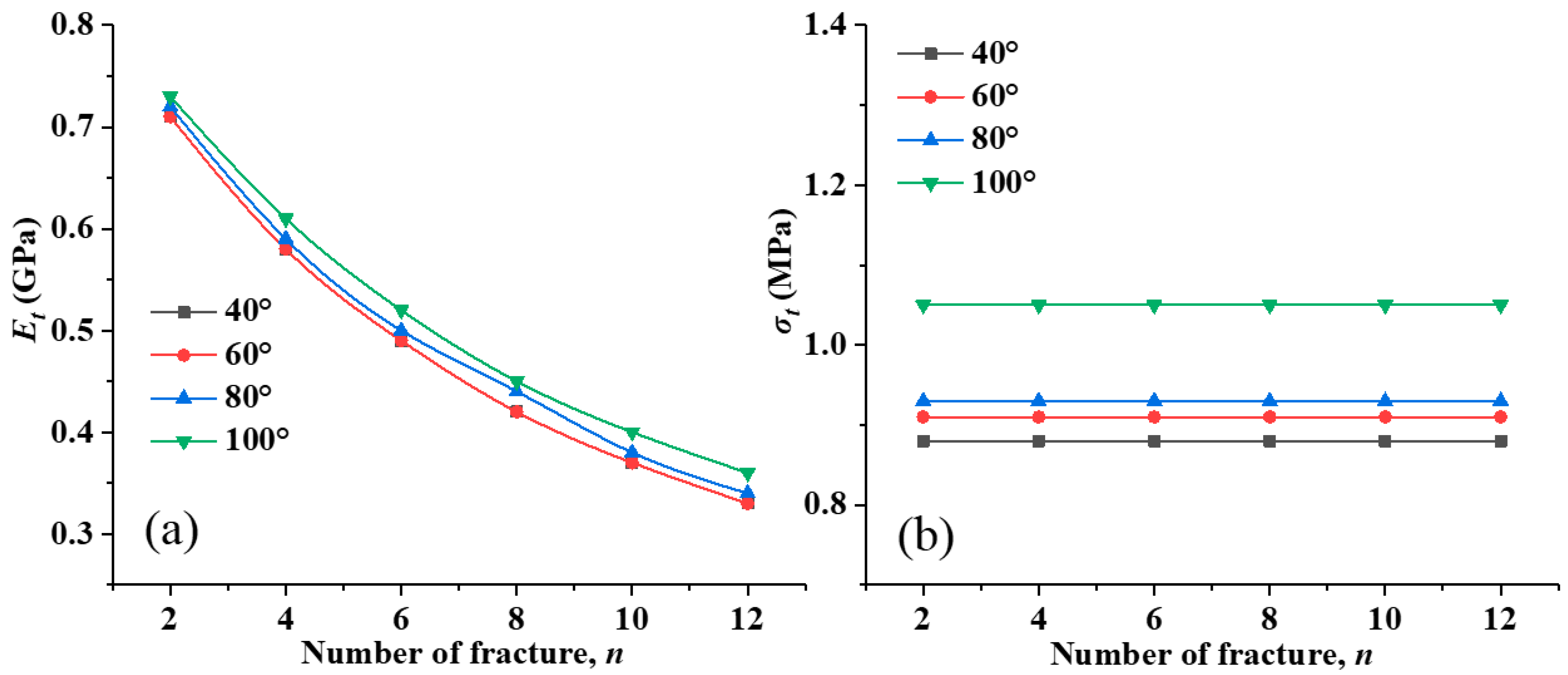
As can be seen, for each subset with the same α, the peaks of the curves are almost identical while the slopes are notably effected by n. Taking the model set with β = 80° as an example, as listed in Figure 15, when n increases from 2 to 12, Et significantly drops from 0.73 to 0.34 GPa, while σt remains constant. The influencing pattern of n on Et is identical for different values of α. These results indicate that the fracture intensity of a rock mass has a great effect on Et but a negligible effect on σt.
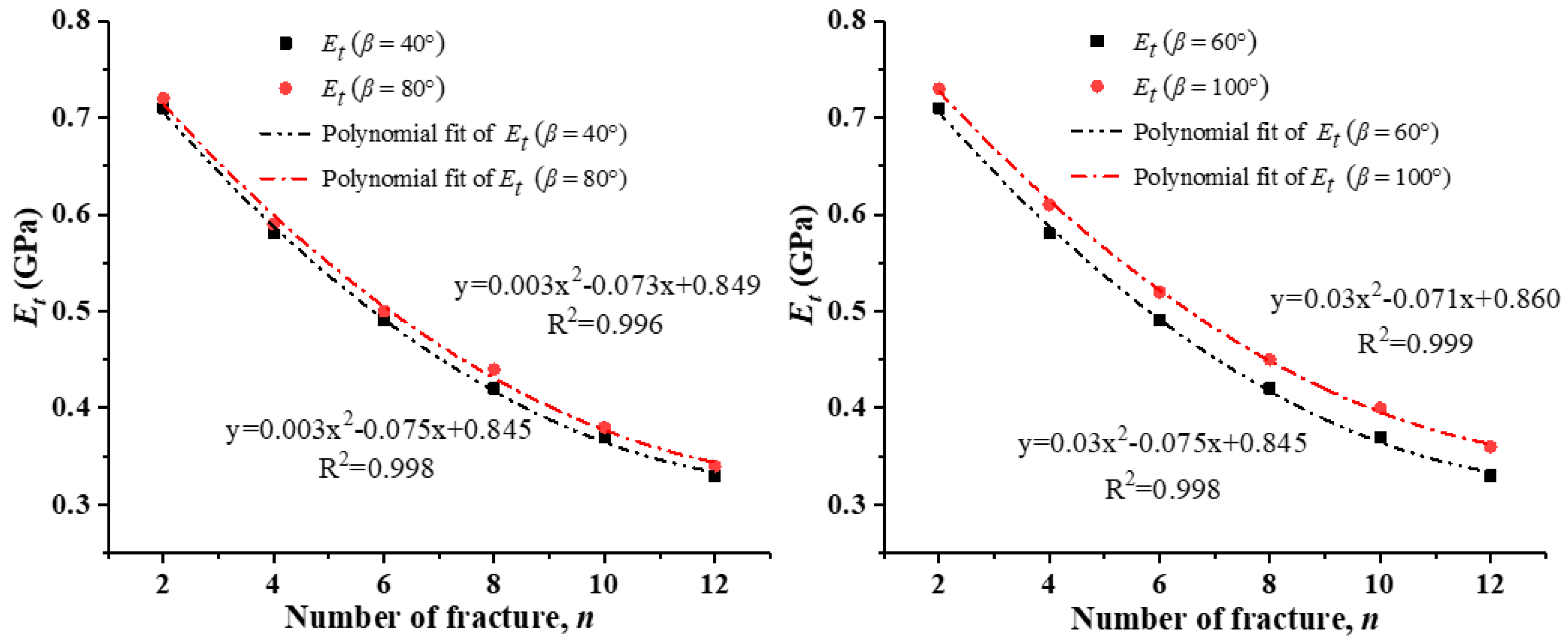
The relationship between n and Et with different values of β after fitting is shown in Figure 16. As can be seen, Et is negatively correlated to n, and the relationship varies with different values of β. The change in Et with n will be less significant in case of a higher value of β.
4. Discussion
The aforementioned results were obtained under the premise that joint development is not considered. In practice, joints will develop, and adjacent joints will connect and merge under mechanical loading. However, this study focuses on the effect of existing joints on the tensile properties.
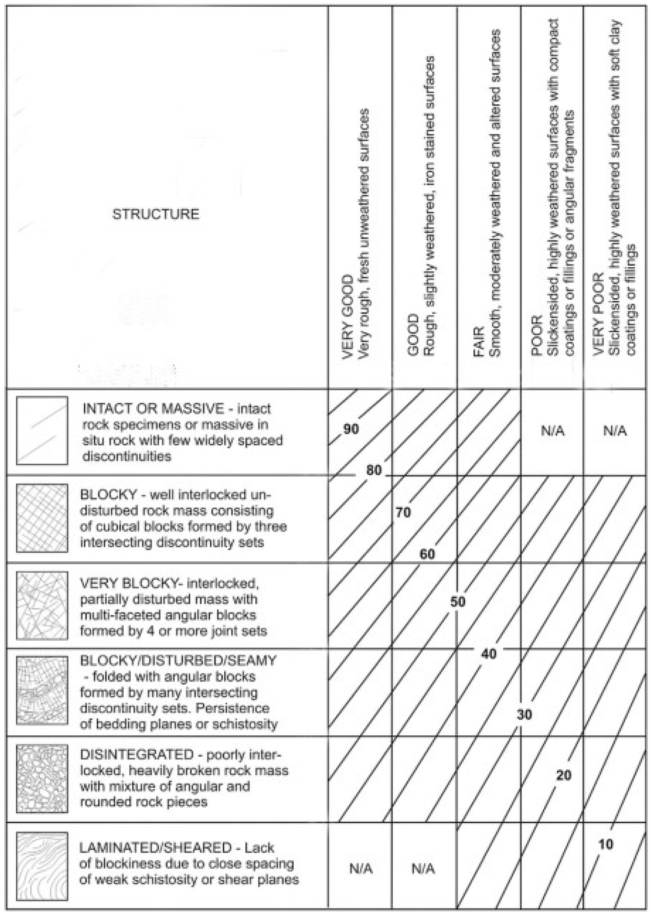
The change in the number of joints can be considered as a change in the degree of development of fractures of the rock mass. Then, the geological strength index (GSI) is introduced [10]. GSI is generally used to calculate the strength and Young’s modulus of a rock mass through laboratory rock mechanics properties and rock mass structural surface parameters. Figure 17 [38] is a GSI quantization table based on rock mass structures and surface features of the structures.
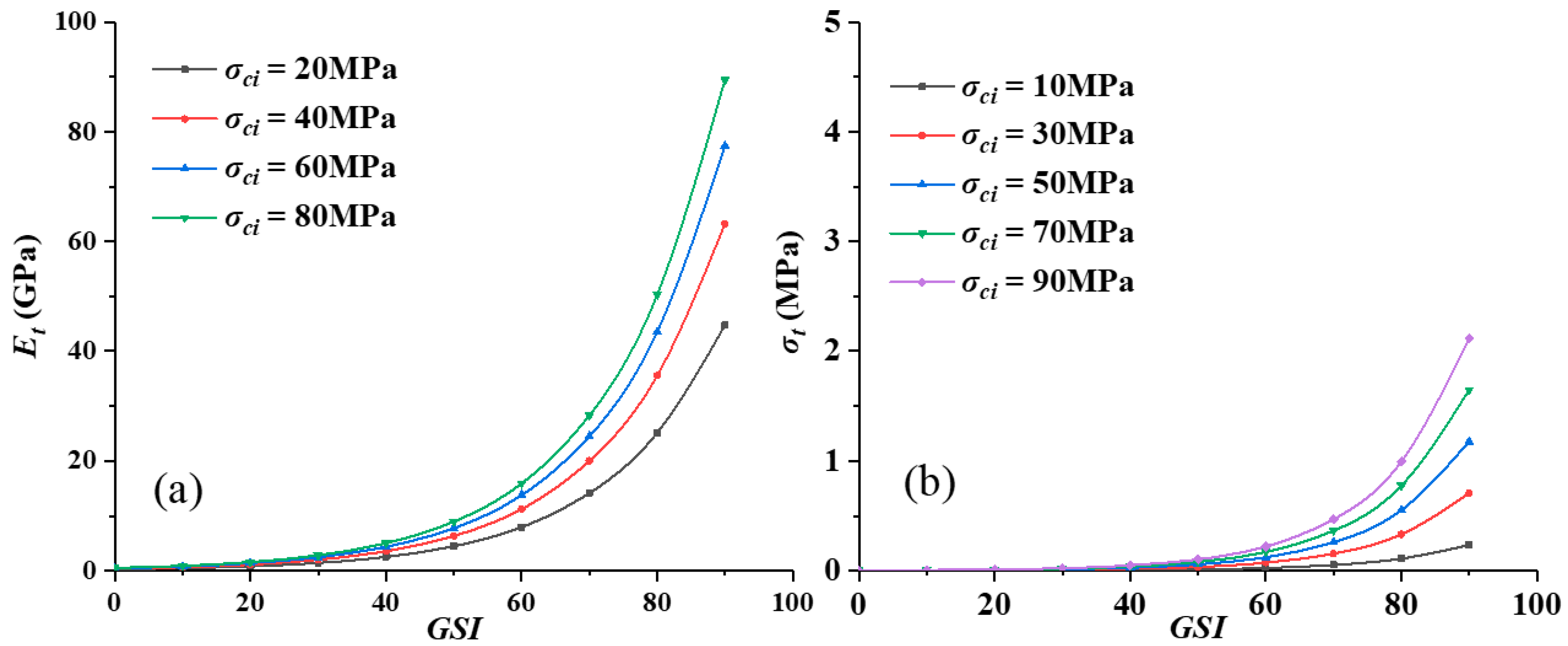
For rocks with a uniaxial compressive strength (σci) < 100 MPa, the elastic modulus of a rock mass (Et) is estimated from the following equation [39]:
where σci is the uniaxial compressive strength of intact rock, and D is a factor that depends on the degree of disturbance to which the rock mass has been subjected by blast damage and stress relaxation. When D = 0, the relationships between Et and GSI under the conditions of different values of σci are shown in Figure 18a. With the increase of the development of rock mass fissures, the Young’s moduli decline notably. The degradation patterns with the number of parallel and intersection joints are illustrated in Figure 19a and Figure 20a, respectively, which agree with the numerical results presented in the previous sections.
According to the generalized Hoek–Brown peak strength criterion [40], the tensile strength of a rock mass is:
where mb is the reduced value of the material constant mi for the rock mass, and is given by:
and s is the rock mass constants, given by:
When D = 0, the relationships between σt and GSI under the conditions of different values of σci are shown in Figure 18b. In a certain interval, the influence on the tensile strength is negligible with the increase of the development of rock mass fissures. Then, the rationalities of the conclusion in this paper were proved, as illustrated in Figure 19b and Figure 20b.
5. Conclusions
According to the aforementioned analysis, the following conclusions can be obtained:
- (1)
- For rock specimens with a single joint, the tensile strength (σt) is positively related to the joint angle (α). However, the Young’s modulus in tension (Et) is barely influenced by α.
- (2)
- For rock specimens with parallel joints, the perpendicular distance (d) between the joints has negligible effects on σt and Et. The influencing pattern is similar to the tests with single joints by changing α while keeping d constant. The number of parallel joints, or joint density, has notable effects on Et but few effects on σt.
- (3)
- For rock specimens with intersecting joints, the number of intersecting joints has notable effects on Et but few effects on σt. For a given number of intersecting joints, σt is positively correlated to the angle between two interesting joints (β).
Author Contributions
Writing—original draft preparation: J.S.; writing-review and editing: L.J.; methodology: P.K. and Q.W.
Funding
The research of this study was sponsored by the National Key R&D Program of China (2018YFC0604703), the National Natural Science Foundation of China (51704182, 51774194), the Natural Science Foundation of the Shandong Province (ZR2017BEE050), and the Shandong University of Science and Technology.
Conflicts of Interest
The authors declare no conflict of interest.
References
- Tang, C.A.; Tham, L.G.; Wang, S.H.; Liu, H.; Li, W.H. A numerical study of the influence of heterogeneity on the strength characterization of rock under uniaxial tension. Mech. Mater. 2007, 39, 326–339. [Google Scholar] [CrossRef]
- Brady, B.H.G.; Brown, E.T. Rock mechanics for underground mining; Springer Science & Business Media: Berlin, Germany, 2004. [Google Scholar]
- Shen, B. Development and applications of rock fracture mechanics modelling with FRACOD: A general review. Geosyst. Eng. 2014, 17, 235–252. [Google Scholar] [CrossRef]
- Jiang, L.; Sainoki, A.; Mitri, H.S.; Ma, N.; Liu, H.; Hao, Z. Influence of fracture-induced weakening on coal mine gateroad stability. Int. J. Rock Mech. Min. 2016, 88, 307–317. [Google Scholar] [CrossRef]
- Jiang, L.; Kong, P.; Shu, J.; Fan, K. Numerical analysis of support designs based on a case study of a longwall entry. Rock Mech. Rock Eng. 2019, 1–12. [Google Scholar] [CrossRef]
- Jiang, L.; Wu, Q.S.; Wu, Q.L.; Wang, P.; Xue, Y.; Kong, P.; Gong, B. Fracture failure analysis of hard and thick key layer and its dynamic response characteristics. Eng. Fail. Anal. 2019, 98, 118–130. [Google Scholar] [CrossRef]
- Ni, G.; Xie, H.; Li, S.; Sun, Q.; Huang, D.; Cheng, Y.; Wang, N. The effect of anionic surfactant (SDS) on pore-fracture evolution of acidified coal and its significance for coalbed methane extraction. Adv. Powder Technol. 2019, 30, 940–951. [Google Scholar] [CrossRef]
- Jiang, L.; Wang, P.; Zheng, P.; Luan, H.; Zhang, C. Influence of Different Advancing Directions on Mining Effect Caused by a Fault. Adv. Civ. Eng. 2019, 2019, 1–10. [Google Scholar] [CrossRef]
- Cai, M.; Kaiser, P.K.; Martin, C.D. Quantification of rock mass damage in underground excavations from microseismic event monitoring. Int. J. Rock Mech. Min. 2001, 38, 1135–1145. [Google Scholar] [CrossRef]
- Tajduś, K. New method for determining the elastic parameters of rock mass layers in the region of underground mining influence. Int. J. Rock Mech. Min. 2009, 46, 1296–1305. [Google Scholar] [CrossRef]
- Hoek, E.; Carranza-Torres, C.; Corkum, B. Hoek-Brown failure criterion-2002 edition. Proc. NARMS-Tac 2002, 1, 267–273. [Google Scholar]
- Mitri, H.S.; Edrissi, R.; Henning, J.G. Finite-element modeling of cable-bolted stopes in hard-rock underground mines. SME Trans. 1995, 298, 1897–1902. [Google Scholar]
- Golsanami, N.; Sun, J.; Liu, Y.; Yan, W.; Lianjun, C.; Jiang, L.; Dong, H.; Zong, C.; Wang, H. Distinguishing fractures from matrix pores based on the practical application of rock physics inversion and NMR data: A case study from an unconventional coal reservoir in China. J. Nat. Gas Sci. Eng. 2019, 65, 145–167. [Google Scholar] [CrossRef]
- Hoek, E.; Bieniawski, Z.T. Brittle Fracture Propagation in Rock Under Compression. Int. J. Fracture 1965, 1, 137–155. [Google Scholar] [CrossRef]
- Paliwal, B.; Ramesh, K.T. An interacting micro-crack damage model for failure of brittle materials under compression. J. Mech. Phys. Solids 2008, 56, 896–923. [Google Scholar] [CrossRef]
- Ashby, M.F.; Hallam, S.D. The failure of brittle solids containing small cracks under compressive stress states. Acta Metall. 1986, 34, 497–510. [Google Scholar] [CrossRef]
- Hawkes, I.; Mellor, M.; Gariepy, S. Deformation of rocks under uniaxial tension. Int. J. Rock Mech. Min. Sci. Geomech. Abstr. 1973, 10, 493–507. [Google Scholar] [CrossRef]
- Haimson, B.C.; Tharp, T.M. Stresses around boreholes in bilinear elastic rock. Soc. Petrol. Engrs. J. 1974, 14, 145–151. [Google Scholar] [CrossRef]
- Barla, G.; Goffi, L. Direct tensile testing of anisotropic rocks, Advances in Rock Mechanics. In Proceedings of the 3rd. Congress of International Society for Rock Mechanics, Denver, CO, USA, 1–7 September 1974. [Google Scholar]
- Chen, R.; Stimpson, B. Interpretation of indirect tensile strength tests when moduli of deformation in compression and in tension are different. Rock Mech. Rock Eng. 1993, 26, 183–189. [Google Scholar] [CrossRef]
- Fuenkajorn, K.; Klanphumeesri, S. Laboratory Determination of Direct Tensile Strength and Deformability of Intact Rocks. Geotech. Test. J. 2010, 34, 103–134. [Google Scholar]
- Yu, X.B.; Xie, Q.; Li, X.Y.; Na, Y.K.; Song, Z.P. Cycle loading tests of rock samples under direct tension and compression and bi-modular constitutive model. Chin. J. Geotech. Eng. 2005, 9, 988–993. [Google Scholar]
- Sundaram, P.N.; Corrales, J.M. Brazilian tensile strength of rocks with different elastic properties in tension and compression. Int. J. Rock Mech. Min. Sci. Geomech. Abstr. 1980, 17, 131–133. [Google Scholar] [CrossRef]
- Okubo, S.; Fukui, K. Complete stress-strain curves for various rock types in uniaxial tension. Int. J. Rock Mech. Min. Sci. Geomech. Abstr. 1996, 33, 549–556. [Google Scholar] [CrossRef]
- Fahimifar, A.; Malekpour, M. Experimental and numerical analysis of indirect and direct tensile strength using fracture mechanics concepts. B. Eng. Geol. Environ. 2012, 71, 269–283. [Google Scholar] [CrossRef]
- Fuenkajorn, K.; Kenkhunthod, N. Influence of Loading Rate on Deformability and Compressive Strength of Three Thai Sandstones. Geotech. Geol. Eng. 2010, 28, 707–715. [Google Scholar] [CrossRef]
- Wang, S.Y.; Sloan, S.W.; Sheng, D.C.; Tang, C.A. 3D numerical analysis of crack propagation of heterogeneous notched rock under uniaxial tension. Tectonophysics 2016, 677–678, 45–67. [Google Scholar] [CrossRef]
- Hamdi, J.; Souley, M.; Scholtès, L.; Heib, M.A.; Gunzburger, Y. Assessment of the Energy Balance of Rock Masses through Discrete Element Modelling. Procedia Eng. 2017, 191, 442–450. [Google Scholar] [CrossRef]
- Guo, L.; Latham, J.P.; Xiang, J. A numerical study of fracture spacing and through-going fracture formation in layered rocks. Int. J. Solids Struct. 2017, 110–111, 44–57. [Google Scholar] [CrossRef]
- Zhou, J.; Li, X.; Mitri, H.S. Evaluation Method of Rockburst: State-of-the-art Literature Review. Tunn. Undergr. Space Technol. 2018, 81, 632–659. [Google Scholar] [CrossRef]
- Chen, L.; Li, P.; Cheng, W.; Liu, Z. Development of cement dust suppression technology during shotcrete in mine of China-A review. J. Loss Prevent. Process Ind. 2018, 55, 232–242. [Google Scholar] [CrossRef]
- Jiang, L.; Zhang, P.; Chen, L.; Hao, Z.; Sainoki, A.; Mitri, H.S.; Wang, Q. Numerical Approach for Goaf-Side Entry Layout and Yield Pillar Design in Fractured Ground Conditions. Rock Mech. Rock Eng. 2017, 50, 3049–3071. [Google Scholar] [CrossRef]
- ISRM. The Complete ISRM Suggested Methods for Rock Characterization, Testing and Monitoring:1974-2006; Ulusay, R., Hudson, J.A., Eds.; Suggested Methods Prepared by the Commission on Testing Methods, International Society for Rock Mechanics, Compilation Arranged by the ISRM Turkish National Group: Ankara, Turkey, 2007.
- Wang, X.; Kulatilake, P.H.S.W.; Song, W. Stability investigations around a mine tunnel through three-dimensional discontinuum and continuum stress analyses. Tunn. Undergr. Space Tech. 2012, 32, 98–112. [Google Scholar] [CrossRef]
- Barton, N. The shear strength of rock and rock joints. Int. J. Rock Mech. Min. Sci. Geomech. Abstr. 1976, 13, 255–279. [Google Scholar] [CrossRef]
- Haftani, M.; Chehreh, H.A.; Mehinrad, A.; Binazadeh, K. Practical Investigations on Use of Weighted Joint Density to Decrease the Limitations of RQD Measurements. Rock Mech. Rock Eng. 2016, 49, 1551–1558. [Google Scholar] [CrossRef]
- Yang, W.; Zhang, Q.; Ranjith, P.G.; Yu, R.; Luo, G.; Huang, C.; Wang, G. A damage mechanical model applied to analysis of mechanical properties of jointed rock masses. Tunn. Undergr. Space Tech. 2019, 84, 113–128. [Google Scholar] [CrossRef]
- Hoek, E.; Marinos, P.G. Predicting tunnel squeezing problems in weak heterogeneous rock masses. Tunn. Tunn. Int. 2000, 132, 45–51. [Google Scholar]
- Wang, P.; Jiang, L.; Li, X.; Qin, G.; Wang, E. Physical simulation of mining effect caused by a fault tectonic. Arab. J. Geosci. 2018, 11. [Google Scholar] [CrossRef]
- Hoek, E.; Brown, E.T. Practical estimates of rock mass strength. Int. Rock Mech. Min. 1997, 34, 1165–1186. [Google Scholar] [CrossRef]
Figure 1.
Rock specimen model with a single joint.

Figure 2.
Mechanical behaviors of single-jointed rock specimens with different dip angles.

Figure 3.
The relationship between joint dip angle α and σt.

Figure 4.
Rock specimen model with parallel joints.

Figure 5.
Tensile behaviors of double-jointed rock specimens with different joint dip angles.

Figure 6.
Rock specimen model with multiple parallel joints.

Figure 7.
Tensile behaviors of rock specimens with different numbers of joints.

Figure 8.
The relationship between the joint density (n) and Et under the different values of α.

Figure 9.
Rock specimen model with intersection joints.

Figure 10.
Tensile behaviors of intersection-jointed rock specimens with different joint angles.

Figure 11.
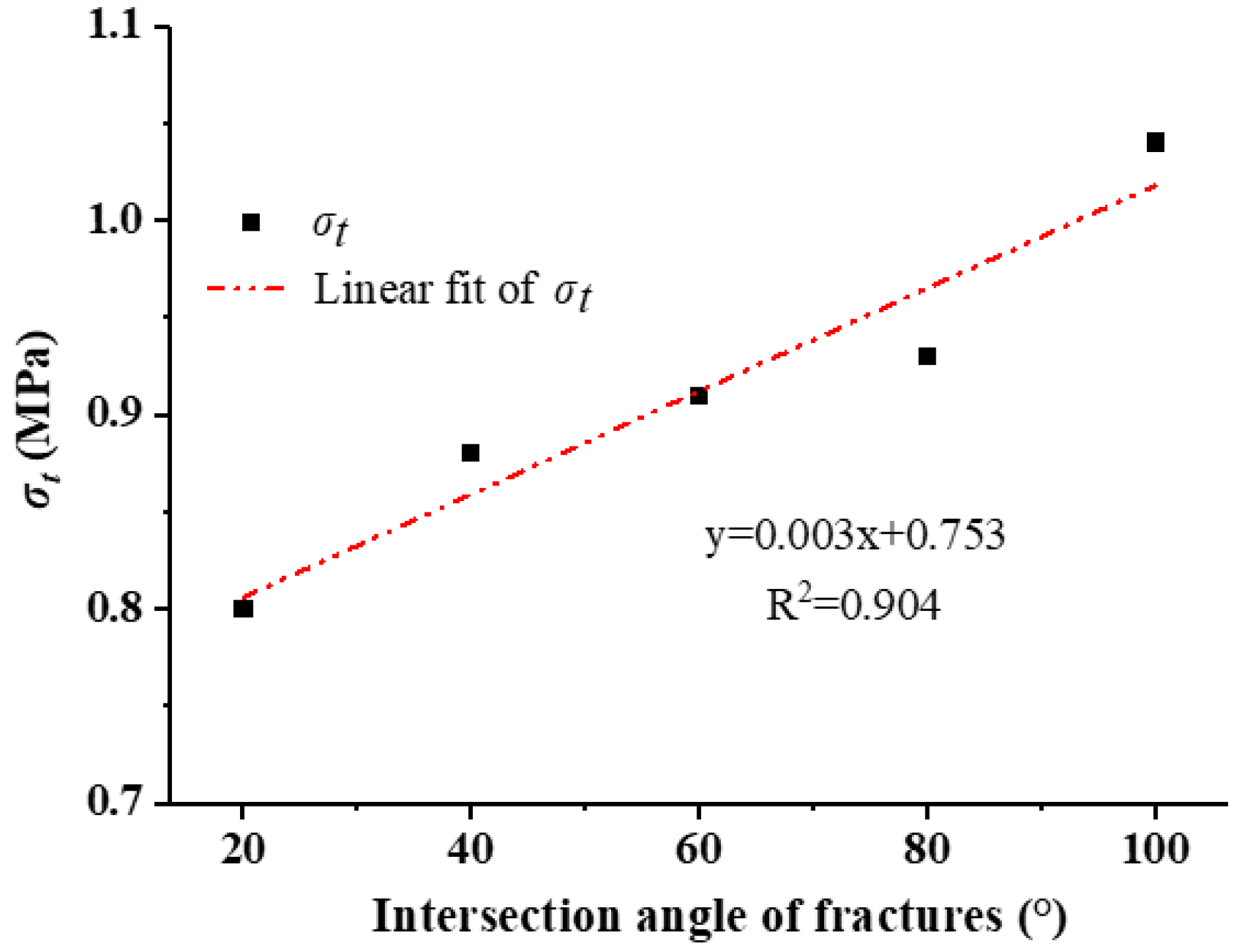
The relationship between the joint intersection angle (β) and σt.

Figure 12.
Rock specimen model with two intersection joints sets .

Figure 13.
Tensile behaviors of intersection-jointed rock specimens with different intersection angles.
Figure 13.
Tensile behaviors of intersection-jointed rock specimens with different intersection angles.

Figure 14.
Rock specimen model with intersecting joints.

Figure 15.
Tensile behaviors of intersection-jointed rock specimens with different numbers of intersection joints.
Figure 15.
Tensile behaviors of intersection-jointed rock specimens with different numbers of intersection joints.

Figure 16.
The relationship between n and Et under the different values of β.

Figure 17.
Quantitative chart of the geological strength index (GSI).

Figure 18.
The effect of GSI onEt, and σt of rock mass (a) Relationship between GSI and Et, (b) Relationship between GSI and σt.
Figure 18.
The effect of GSI onEt, and σt of rock mass (a) Relationship between GSI and Et, (b) Relationship between GSI and σt.

Figure 19.
Effect of the number of parallel fractures on Et and σt. (a) Effect of the number of fractures on Et ,(b) Effect of the number of fractures on σt.
Figure 19.
Effect of the number of parallel fractures on Et and σt. (a) Effect of the number of fractures on Et ,(b) Effect of the number of fractures on σt.

Figure 20.
Effect of the number of intersecting parallel fractures on Et and σt. (a) Effect of the number of fractures on Et, (b) Effect of the number of fractures on σt.
Figure 20.
Effect of the number of intersecting parallel fractures on Et and σt. (a) Effect of the number of fractures on Et, (b) Effect of the number of fractures on σt.


Table 1.
Rock mass properties.
| Lithology | Density (kg/m3) | Bulk modulus K (GPa) | Shear modulus G (GPa) | Cohesion C (MPa) | Internal friction angle φ (°) | Tensile strength (MPa) |
|---|---|---|---|---|---|---|
| Sandstone | 2630 | 26.49 | 19.05 | 3.75 | 25.9 | 2.25 |
Table 2.
Joint properties.
| Lithology | Cohesion C (MPa) | JKN (GPa/M) | JKS (GPa/M) | Joint friction angle (°) | Tensile strength (MPa) |
|---|---|---|---|---|---|
| Sandstone | 3.67 | 26.49 | 19.05 | 25.9 | 1.88 |
Table 3.
Tensile strengths (σt) and Young’s moduli in tension (Et) of single-jointed rock specimens with different dip angles.
Table 3.
Tensile strengths (σt) and Young’s moduli in tension (Et) of single-jointed rock specimens with different dip angles.
| α | σt (MPa) | Et (GPa) |
|---|---|---|
| α = 0° | 0.78 | 0.80 |
| α = 10° | 0.80 | 0.80 |
| α = 20° | 0.88 | 0.80 |
| α = 30° | 0.91 | 0.80 |
| α = 40° | 0.93 | 0.81 |
| α = 50° | 1.05 | 0.81 |
Table 4.
Model designs for rock specimens with two parallel joints.
| Sets of models | α | Subsets with respect to d |
|---|---|---|
| 1 | 20° | 10 mm |
| 20 mm | ||
| 30 mm | ||
| 40 mm | ||
| 2 | 30° | 10 mm |
| 20 mm | ||
| 30 mm | ||
| 40 mm | ||
| 3 | 40° | 10 mm |
| 20 mm | ||
| 30 mm | ||
| 40 mm | ||
| 4 | 50° | 10 mm |
| 20 mm | ||
| 30 mm | ||
| 40 mm |
Table 5.
Tensile properties of double-jointed rock specimens with different joint dip angles.
| α | σt (MPa) | Et (GPa) |
|---|---|---|
| 20° | 0.88 | 0.71 |
| 30° | 0.91 | 0.71 |
| 40° | 0.93 | 0.73 |
| 50° | 1.05 | 0.73 |
Table 6.
Model designs for rock specimens with multiple parallel joints.
| Sets of models | α | Subsets with respect to n |
|---|---|---|
| 1 | 20° | n = 2 |
| n = 3 | ||
| n = 4 | ||
| n = 5 | ||
| 2 | 30° | n = 2 |
| n = 3 | ||
| n = 4 | ||
| n = 5 | ||
| 3 | 40° | n = 2 |
| n = 3 | ||
| n = 4 | ||
| n = 5 | ||
| 4 | 50° | n = 2 |
| n = 3 | ||
| n = 4 | ||
| n = 5 |
Table 7.
Effect of joint density of parallel joints on tensile properties.
| n | σt (MPa) | Et (GPa) |
|---|---|---|
| n = 1 | 0.93 | 0.81 |
| n = 2 | 0.93 | 0.73 |
| n = 3 | 0.93 | 0.66 |
| n = 4 | 0.93 | 0.61 |
| n = 5 | 0.93 | 0.56 |
| n = 6 | 0.93 | 0.52 |
Table 8.
σt and Et of intersection-jointed rock specimens with different joint angles.
| α | σt (MPa) | Et (GPa) |
|---|---|---|
| β = 20° | 0.80 | 0.71 |
| β = 40° | 0.88 | 0.71 |
| β = 60° | 0.91 | 0.71 |
| β = 80° | 0.93 | 0.73 |
| β = 100° | 1.05 | 0.73 |
Table 9.
Model designs for rock specimens with two intersecting joint sets.
| Sets of Models | d | Subsets with Respect to β |
|---|---|---|
| 1 | d = 10 mm | β = 40° |
| β = 60° | ||
| β = 80° | ||
| β = 100° | ||
| 2 | d = 20 mm | β = 40° |
| β = 60° | ||
| β = 80° | ||
| β = 100° | ||
| 3 | d = 30 mm | β = 40° |
| β = 60° | ||
| β = 80° | ||
| β = 100° | ||
| 4 | d = 40 mm | β = 40° |
| β = 60° | ||
| β = 80° | ||
| β = 100° |
Table 10.
σt and Et of intersection-jointed rock specimens with different intersection angles.
| β. | σt (MPa) | Et (GPa) |
|---|---|---|
| β = 40° | 0.88 | 0.58 |
| β = 60° | 0.91 | 0.58 |
| β = 80° | 0.93 | 0.58 |
| β = 100° | 1.05 | 0.61 |
Table 11.
Model designs for rock specimens with two parallel joints.
| Sets of Models | β | Subsets with Respect to n |
|---|---|---|
| 1 | 40° | n = 4 |
| n = 6 | ||
| n = 8 | ||
| n = 10 | ||
| n = 12 | ||
| 2 | 60° | n = 4 |
| n = 6 | ||
| n = 8 | ||
| n = 10 | ||
| n = 12 | ||
| 3 | 80° | n = 4 |
| n = 6 | ||
| n = 8 | ||
| n = 10 | ||
| n = 12 | ||
| 4 | 100° | n = 4 |
| n = 6 | ||
| n = 8 | ||
| n = 10 | ||
| n = 12 |
Table 12.
Mechanical behaviors of rock specimens with different numbers of intersection joints.
| n | σt (MPa) | Et (GPa) |
|---|---|---|
| n = 2 | 0.93 | 0.73 |
| n = 4 | 0.93 | 0.58 |
| n = 6 | 0.93 | 0.50 |
| n = 8 | 0.93 | 0.44 |
| n = 10 | 0.93 | 0.38 |
| n = 12 | 0.93 | 0.34 |
© 2019 by the authors. Licensee MDPI, Basel, Switzerland. This article is an open access article distributed under the terms and conditions of the Creative Commons Attribution (CC BY) license (http://creativecommons.org/licenses/by/4.0/).
Share and Cite
MDPI and ACS Style
Shu, J.; Jiang, L.; Kong, P.; Wang, Q. Numerical Analysis of the Mechanical Behaviors of Various Jointed Rocks under Uniaxial Tension Loading. Appl. Sci. 2019, 9, 1824. https://doi.org/10.3390/app9091824
AMA Style
Shu J, Jiang L, Kong P, Wang Q. Numerical Analysis of the Mechanical Behaviors of Various Jointed Rocks under Uniaxial Tension Loading. Applied Sciences. 2019; 9(9):1824. https://doi.org/10.3390/app9091824
Chicago/Turabian StyleShu, Jiaming, Lishuai Jiang, Peng Kong, and Qingbiao Wang. 2019. "Numerical Analysis of the Mechanical Behaviors of Various Jointed Rocks under Uniaxial Tension Loading" Applied Sciences 9, no. 9: 1824. https://doi.org/10.3390/app9091824
Note that from the first issue of 2016, this journal uses article numbers instead of page numbers. See further details here.