A Compact Bat Algorithm for Unequal Clustering in Wireless Sensor Networks

Abstract

Everyday, a large number of complex scientific and industrial problems involve finding an optimal solution in a large solution space. A challenging task for several optimizations is not only the combinatorial operation but also the constraints of available devices. This paper proposes a novel optimization algorithm, namely the compact bat algorithm (cBA), to use for the class of optimization problems involving devices which have limited hardware resources. A real-valued prototype vector is used for the probabilistic operations to generate each candidate for the solution of the optimization of the cBA. The proposed cBA is extensively evaluated on several continuous multimodal functions as well as the unequal clustering of wireless sensor network (uWSN) problems. Experimental results demonstrate that the proposed algorithm achieves an effective way to use limited memory devices and provides competitive results.

1. Introduction

The metaheuristic algorithms have emerged as a potential tool for solving complex optimization problems. The bat algorithm (BA) is a novel metaheuristic search algorithm [1,2], which simulates the behavior of the bat species for searching prey. Preliminary studies show that it is very promising and could outperform existing algorithms [3]. The BA utilizes a population of bats to represent candidate solutions in a search space and optimizes the problem by iteration to move these agents to the best solutions about a given measure of quality. The general steps of this algorithm are described in the next section.

The original BA is able to solve problems with continuous search space, and in addition, several versions of the algorithm are also proposed in the literature to solve problems with continuous and discrete search spaces. The evolved bat algorithm (EBA) is used for numerical optimization and the economic load dispatch problem [4,5]. A hybrid between the BA and the artificial bee colony (ABC) is used for solving numerical optimization problems [6]. Several discrete BAs have been proposed in the literature, in addition to the continuous BAs. A binary BA (BBA) was proposed to solve the feature selection problem [7], and its solution is restricted to a vector of binary positions using a sigmoid function. The BBA algorithm uses a V-shaped transfer function to map velocity values to probability values in order to update the positions [8]. This BBA has been used in several tasks, e.g., it was adopted in [9] as the feature selection part of a fault diagnosis scheme for failures of incipient low-speed rolling element bearings. As another example, a chaotic version of the algorithm, namely CBBA, was used to select points in an analog circuit diagnosis system [10]. A similar BBA algorithm, with a multi V-shaped version of the transfer function, was adopted in order to solve a large scale 0–1 knapsack problem [11]. A discrete version of BA was parallelized (called PBA) for optimizing makespan in job shop scheduling problems [12]. Another discrete BA was used to address the optimal permutation of the flow shop scheduling problem [13] and discrete BA was adopted to solve the symmetric and asymmetric Traveling salesman problem (TSP) [14].

Moreover, rapid growth in the field of integrated circuits (IC) and information technology (IT) has led to the development of inexpensive and tiny-size sensor nodes in a wireless sensor network (WSN). A WSN is composed of a vast number of sensor nodes arranged in an ad hoc fashion to observe and interact with the physical world [15]. The sensors capture the environmental information which is processed and forwarded to the base station (BS) via middle nodes or single hop [16]. A WSN detects and measures (or monitors) a number of physical or environmental conditions such as multimedia [17,18], infrared energy emitted from objects and converted to temperature [19], pollutant levels [20], ultrasound in medical imaging [21], vibrations [22], security and surveillance [23], agriculture [24], and many other such conditions. Usually, a WSN is carried out in areas that are difficult to access and intervention is not possible by people. In a harsh environment, it is difficult or not possible to recharge or replace batteries used in the sensors of a WSN [25]. The energy consumption, memory, and bandwidth are the key factors that influence a good WSN design.

Applications of WSNs have become widely accessible in some fields, e.g., military surveillance, agriculture, disaster management, healthcare monitoring, industry automation, inventory control, and so forth [26,27]. However, WSNs are networks of small, battery-powered, memory-constrained sensor nodes. Sensor nodes in WSN are an example of hardware devices that are limited by conditions due to the cost, storage, and space restriction. The optimization problem with a limited hardware resource becomes a challenging one [25].

Furthermore, in this paper one of our goals is based on a theorem of “no free lunch” which states that there is no metaheuristic algorithm best suited for solving all optimization problems [28]. It means that one algorithm might obtain excellent results on a given set of challenges but underperform on an alternative set of issues. Another goal in this paper is to consider the strength of different algorithms based on the types and properties of the problem.

In this paper, we extend our previous work of the compact bat algorithm (cBA) [2] for the unequal clustering of wireless sensor networks (uWSN) problems. By extending our work we aim to deal with the issues of saving variable memory and selecting parameters according to the unequal clustering problem of WSNs. The reasons for extending our work include an added need to control the probability of sampling for perturbation vector, a set of tests for benchmark functions, a solution to the unequal clustering problem, and an extensive comparison with other compact algorithms in the literature. A real-valued prototype vector is used for the probabilistic operations to generate each candidate for solving the optimization of the cBA. The proposed cBA is extensively evaluated on several continuous multimodal functions as well as the unequal clustering of wireless sensor network (uWSN) problems.

2. Related Work

2.1. Unequal Clustering in Wireless Sensor Network (WSN)

Clustering and unequal clustering techniques have been used for an energy efficient WSN. Clusters in WSNs are carried out by grouping sensor nodes into a partitioned set. One of the nodes in the partitioned set is selected to be a cluster head (CH) that collects information from the cluster member nodes (CNs) [16,29]. Energy consumption of the CHs near the base station (BS) is more than the CHs farther from the BS. This means CHs close to the BS have a heavy traffic load because of intra-cluster traffic from its cluster members, data aggregation, and inter-cluster traffic from other CHs for relaying data to the BS. This disrupts the network connectivity, and the clusters close to the BS cause coverage issues that are called hot spot problems. The unequal clustering technique is one of the most efficient ways to deal with hot spot problems because it can be used for load balancing among the CHs [30].

The purpose of the unequal clustering method is the same as the equal clustering approach with adding functions. The clustered nodes are in WSN for different meanings based on the application demand. Energy saving and preventing hot spot problems are the major objectives. Unequal clustering arranges the clusters according to size with the size reduced closer to the BS. This means that the cluster size is directly proportional to the distance of the CHs from the BS. A smaller cluster near the BS indicates a smaller number of cluster members and less intra-cluster traffic. Therefore, the smaller clusters can concentrate more on inter-cluster traffic, and the cluster head does not drain out of energy as quickly. The more the distance to the BS increases, the more the cluster size increases. If the groups hold a more significant number of member nodes, they will spend more energy on intra-cluster traffic. As the clusters become farther from the BS, they have less inter-cluster traffic and do not need to expend more energy for inter-cluster routing. Unequal clustering forces all the CHs to spend the same amount of energy consumption, and therefore the CHs near the BS and the CHs farther from the BS consume an equal amount of energy.

Additionally, the cluster formation process may generate a two-level hierarchy with higher and lower levels [31,32]. The CH nodes form the upper-level cluster, and the member nodes create the lower level. The sensor nodes periodically transmit their data to the corresponding CH. The CHs aggregate the data and transmit them to the BS either directly or through the intermediate CH nodes. The CH performs data aggregation of all data received from its cluster members and forwards the aggregated data to the BS via a single hop or a multi-hop. The CH contains the information of its cluster members such as node id, location, and energy level. When a node dies or moves to another cluster, the changes are registered immediately and the CH informs the BS and reclustering occurs to maintain the network topology effectively. The number of transmissions and also the total load of the network are significantly reduced.

2.2. Energy Consumption in WSNs Model

Unequal clustering in a WSN with hundreds or thousands of sensor nodes is an efficient way to organize such a vast number of nodes, uniformly distribute load, and prevent hot spot problems [33]. However, the equal clustering approach often has cluster size which is the same throughout the network. Admittedly, in unequal clustering, the cluster size is determined based on the distance to the BS. The cluster size is smaller when the distance to the BS is shorter, and the size increases as the distance to the BS increases.

The wireless radio transceiver in a WSN depends on the various parameters, e.g., distance and energy consumption. The definition is related to the power consumption and the ranges of the nodes referred to in [16]. The distance between the transmitter and receiver obeyed on the attenuated trans-receiving power decreases exponentially with increasing distance. A threshold separates the free space model and the multipath model.

$$d_0= \sqrt{\left(\left({\epsilon }_{fs}\right)/{\epsilon }_{mp}\right)}$$

(1)

where ${\epsilon }_{fs}$, ${\epsilon }_{mp}$ are power loss for free space and multipath models, respectively, and $d_0$ is a threshold of space model. The transmitting l bits for dissipated energy over distance d is formulated as:

$$E_{Tx\left(l,d\right)}=E_{Tx-elec}\left(l\right)+E_{Tx-amp}\left(l,d\right)=\{\begin{array}{c}l\times E_{elec}+l\times {\epsilon }_{fs}\times d^2, d>d_o\\ l\times E_{elec}+l\times {\epsilon }_{mp}\times d^4, d\ge d_o\end{array}$$

(2)

where $E$ is the power consumption of the node, Tx is for transmitting subscript elec, amp indicate electronic, and amplify for digital coding, modulating, filtering, and spreading signal. The energy consumption for receiving the messages can be expressed as:

$$E_{Rx}\left(l\right)= E_{Rx \_elec}\left(l\right)=l\times E_{elec}$$

(3)

WSN assumed implemented N nodes in the two-dimensional area of $M^2$ with k clusters. Let $d$ be the distance member node to the CH, and $D$ be the distance of the CHs to the BS. The consumed energy of a cluster for a data frame is modelled as:

$$E_{cluster}=E_{CH}+\left(\frac{N}{k}-1\right)\times E_{member}$$

(4)

where $N/k$ − 1 is the averaged member nodes in a cluster. $E_{CH}$ and $E_{members}$ are the dissipated energy for CH and members. The calculated energy consumptions for cluster members and CHs are as follows:

$$E_{member}=l\times E_{elec}+l\times {\epsilon }_{fs}\times d_{toCH}^2$$

(5)

$$E_{CH}=l\times E_{elec}\times \left(\frac{N}{k}-1\right)+l\times E_{DA}\times \frac{N}{k}+l\times E_{elec}+l\times {\epsilon }_{mp}\times D_j^2$$

(6)

The total consumed energy for a WSN could be formulated from the energy process and power transceiver as:

$$E_{total}=E_p+E_{frame}= E_p+k\times E_{cluster}$$

(7)

where $E_p$ is the power consumption of the microcontroller. It does not affect the optimizing processes. Thus, the power consumption of $E_{frame}$ optimized is based on only the distance for clustering optimization.

3. Compact Bat Algorithm

The compact approach reproduces the operations of the population-based algorithms by building a probabilistic model for a population solution. The optimal process considers the actual population as a virtual community by encoding its probabilistic representation. The compact BA is constructed based on the framework of the BA. Before analyzing and designing the compact for BA, we review the bat-inspired algorithm in the following subsection.

3.1. Bat-Inspired Algorithm

A recent new population-based algorithm, BA [1] has drawn inspiration from the bat’s echolocation of the species called the microbats for searching prey. The updated solutions of BA are constructed based on three primary characteristics including echolocation, frequency, and loudness. Bats use echolocation to locate the prey, background frequency to send out the variable wavelength, and loudness to search the victim. Solutions for the BA are generated by adjusting parameters, e.g., frequencies, loudness, and pulse emission rates of the bats, according to the evaluation of the objective function. Formulas for updating the positions and velocities of BA in d-dimensional search space are as follows:

$$f_i=f_{min}+\left(f_{max}-f_{min}\right)\times \beta$$

(8)

where $f_i$ is the frequency for adjusting velocity change, $f$_min and $f$_max the minimum and maximum frequency of the bats emitting the pulse, respectively, and $\beta$ is a generated vector randomly based on the distributed Gaussian ∈ [0, 1]. A frequency assigned initially for each bat in a uniform range ∈ [$f$_min, $f$_max]. BA updates the vectors of the bat locations and velocity x, and v in search space of d-dimensional.

$$v_i^t=v_i^{t-1}+\left(x_i^{t-1}-x_{best}\right)\times f_i,$$

(9)

$$x_i^t=x_i^{t-1}+v_i^t,$$

(10)

where the superscript of $t$ is the current iteration, and $x_{best}$ is the global best solution. Generating new location of the bats in exploiting phase strategy is formulated as:

$$x_i=x_i+\epsilon \times A^t,$$

(11)

where $\epsilon$ is a random variable in the range $\in [-1, 1]$, and indicates the weight for the loudness of the bats at the current generation. The loudness of bats $A$ is defined as:

$$A_{ i}^{t+1}= \alpha \times A_{i }^t,$$

(12)

where α is a variable constant. The symbol denotes the rate of the pulse emission $r$ and ∈ [0, 1]. The pulse emission rate is calculated as:

$$r_i^{t+1}=r_i^0\times \left[1-e^{-\gamma \times t}\right],$$

(13)

where $\gamma$ is the constant variable. In the process, this rate $r$ is considered as the control to switch the global and local search. If a random number is greater than $r$, a local search with a random walk is triggered.

3.2. Compact Bat Algorithm

The intention of the compact algorithm is to mimic the operations of the based-population algorithm of BA in a version with a much smaller stored variable memory. The actual population of solutions of the BA is transformed into the compact algorithm by constructing a distributed data structure, namely the perturbation vector (PV). PV is the probabilistic model for a population of solutions.

$$P{V}^t= \left[{\mu }^t,{\delta }^t\right],$$

(14)

where $\delta$ and $\mu$ are two parameters of standard deviation and mean of vector PV, and t is the current time. The values of $\delta$ and $\mu$ are arranged within the probability density functions (PDF) [34] and are truncated in [−1, 1]. The amplitude of PDF is normalized by keeping its area equal to 1 because by obtaining approximately sufficient in well it is the uniform distribution with a full shape.

A real-valued prototype vector is used to maintain sampling probabilistic for randomly generating components of a candidate solution. This vector operation is distributed-based on the estimated distribution algorithm (EDA) [35]. Because a few new generating candidates are stored in the memory, it is not all of the population of solutions stored in memory. The likelihood is that the estimated distribution would trend, driving new candidate forward to the fitness function. Candidate solutions are generated probabilistically from the vector, and the components in the better solution are used to make small changes to the probabilities within the vector. A candidate solution $x_i$ corresponding to the location of the virtual bats is generated by $PV\left({\mu }_i,{\delta }_i\right)$.

$$P\left(\mathrm{x}\right)=\frac{ex{p}^{\frac{{\left(x-{\mu }_i\right)}^2}{2{\delta }_i^2}}}{{\delta }_i\left(\mathrm{erf}\left(\frac{{\mu }_i+1}{\sqrt{2}{\delta }_i}\right)-\mathrm{erf}\left(\frac{{\mu }_i+1}{\sqrt{2}{\delta }_i}\right)\right)}$$

(15)

where $P\left(\mathrm{x}\right)$ is the probability distribution of $PV$ that formulated a truncated Gaussian PDF associated with the $\mu$ and $\delta$. A new candidate solution is generated by being iteratively biased toward a promising area of an optimal solution. We can obtain each component of the probability vector by learning the previous generations. The $erf$ is the error function found in [36]. PDF corresponds to the cumulative distribution function (CDF) by constructing Chebyshev polynomials [37]. The codomain of $CDF$ is arranged from 0 to 1. The $CDF$ can describe the real-valued random variable x with a given probability distribution, and the obtained value can be less than or equal to $x_i.$

CDFs also can specify the distribution of multivariate random variables. Thus, the relationship of PDF and CDF can be defined as $CDF={\int }_0^{1}P\left(x\right)dx$. PV performs the sampling design variable $x_i$ by generating a random number in a range of (0, 1). This corresponds to obtaining this variable by computing the inverse function of $x_i$ set to inverse (CDF).

To find the better individual in the process of the compact algorithm, a comparison of the two design variables is conducted. The two variable agents of the bats are two sampled individuals who performed from PV. The “winner” indicates the vector with the fitness scores that are higher than other members, and the “loser” is shown according to the individual lower fitness evaluation. The two returned variables, $winner$ and $loser$, are from objective function evaluation that compare a new candidate with the previous global best. For updating PV, $\mu \mathrm{and}\delta$ are considered based on the following rules. If the mean value of $\mu$ is regarded to 1, the update rule for each of its elements is ${\mu }_i^t,{\delta }_{i }^t \mathrm{set}\mathrm{forward}\mathrm{to}{\mu }_i^{t+ 1},{\delta }_i^{t +1}$ as given in the equation below:

$${\mu }_i^{t+1}={\mu }_i^t+\frac{1}{N_p}\left(winne{r}_i-lose{r}_i\right)$$

(16)

where $N_p$ denotes virtual population. With respect to $\delta$ values, the update rule of each element is given as:

$${\delta }_i^{t+1}=\sqrt{{({\delta }_i^t)}^2+{\left({\mu }_i^t\right)}^2-{\left({\mu }_i^{t+1}\right)}^2+\frac{1}{N_p}\left(winne{r}_i^2-lose{r}_i^2\right)}$$

(17)

$$\left[winner,loser\right]=compete\left(x_{best},x^{t+1}\right)$$

(18)

In general, a probabilistic model for compact BA is employed to represent the bat solution set where neither the location nor the velocities are stored, however, a newly generated candidate is stored. Thus, modest memory space is required, and it is well suited for the limited hardware resources in WSNs.

A parameter $\omega$ is used as a weight to control the probability of sampling of ${\mu }_i$ in PDF as Equation (15) between left [−1, ${\mu }_i$] that is $P_L\left(\mathrm{x}\right), \mathrm{for}-1\le x\le {\mu }_i,$ and right [${\mu }_i$, 1] that is $P_R\left(\mathrm{x}\right), \mathrm{for} {\mu }_i\le x\le 1$. The extended version Equation (15) of PDF for sampling approach is applied in this paper. The generating new candidates of the bats are employed by sampling from $PV$ such as when r < ω then it generates the coefficient $x_i \in [1,0]$ for $P_L\left(\mathrm{x}\right),$ otherwise $x_i\in [1,0]$ for $P_R\left(\mathrm{x}\right)$. The details for compact BA are as follows:

Step 1 Initialization: $\mu$ and $\delta$ of the probabilistic model vector PV.

Step 2 Initialize parameters: the pulse rate $r_i$, the loudness $A$_i, and $\beta$ are set to random; search range definition of pulse frequency $f_{min}, \mathrm{and} f_{max}$.

Step 3 Generate the global best solution $x_{best}$ by means of perturbation vector PV; assign $F$_min to fitness ($x_{best}$).

Step 4 Generate the local best solution $x^t$ from $PV$.

Step 5 Update velocities v^t and locations $x^t$ according to updating rule of the standard BA algorithm, Equations (8)–(10); if ($\beta > r_i$), select a local solution $x^{t+1}$ around selected best solution as Equation (11); assign the function value $F$_new to fitness $\left(x^{t+1}\right).$

Step 6 Compare $x^{t+1}$ and $x_{best}$, let one be the winner, and the other one is the loser according to Equation (16).

Step 7 Update $PV$ according to Equations (17) and (18).

Step 8 A new solution is accepted if the solution improves ($F_{new}$ less than $F_{min}$), and not too loud ($\beta$ less than $A$) then update global best $x_{best}$ to $x^{t+1}$ and assign function $F_{min}$ to $F_{new}$.

Step 9 If the termination condition is not met, go to step 4.

Step 10 Output the global best solution $x_{best}$.

4. Experiments with Numerical Problems

To validate the quality performance of the proposed algorithm, we select ten optimal numerical problems [38] to prove the accuracy and rate of the cBA. The cBA measurements are compared with the original bat algorithm (oBA) with respect to solution quality. The two techniques used to verify the performance of the proposed cBA include similarity measure and time complexity analysis. The similarity measure uses a probability cosine with an adopted Pearson’s correlation coefficient that considers the measured ratio (r) for two result solutions. The time complexity analysis uses the number of related variables employed in the optimization process. All the selected test functions for the outcomes of the experiment averaged over 25 runs. Minimized outcomes of optimization are calculated for all functions. Let X = {x₁, x₂, …, x_n} be the n-population size real-value vector. The related initial data of test functions, i.e., range boundaries, max iteration, and dimension are listed in

Table 1. Ten selected benchmark functions of testing.

Name	Test Functions	Range	Dimension	Iteration
Rosenbrock	$f_1\left(x\right)={\displaystyle \sum _{i=1}^{n-1}}(100\times {\left(x_{i-1}-x_i^2\right)}^2+{\left(1-x_i\right)}^2$	±100	30	5000
Quadric	$f_2\left(x\right)={\displaystyle \sum _{i=1}^n}{\displaystyle \sum _{k=1}^i}{x}_i$	±100	30	5000
Ackley	$f_3\left(x\right)=20+e-20e^{-0.2\sqrt{\frac{{\sum }_{i=1}^n{x}_i^2}{n}}}-e^{\frac{{\sum }_{j=1}^n\cos \left(2\pi x_i\right)}{n}}$	±32	30	5000
Rastrigin	$f_4\left(x\right)={\sum }_{i=1}^N[10+x_i^2-10cos2\pi x_i]$	±5.12	30	5000
Griewangk	$f_5\left(x\right)=1+{\displaystyle \sum _{i=1}^N}\frac{x_i^2}{4000}+{\displaystyle \prod _{i=1}^N}cos\frac{x_i}{\sqrt{i}}$	±100	30	5000
Spherical	$f_6\left(x\right)={\displaystyle \sum _{i=1}^N}{x}_i^2$	±100	30	5000
Quartic Noisy	$f_7\left(x\right)=random[0,1)+{\displaystyle \sum _{i=1}^N}i\times x_i^4$	±1.28	30	5000
Schwefel	$f_8\left(x\right)=418.983n-{\displaystyle \sum _{i=1}^N}{x}_i\times \sin \left(\sqrt{\left|x_i\right|}\right)$	±100	30	5000
Langermann	$f_9(x)={\displaystyle {\sum }_{i=1}^n[x_i^2}-10\cos (2\pi x_i)+10]$	±5.12	30	5000
Shubert	$f_{10}(x)=-20\exp (-0.2\sqrt{\frac{1}{n}{\displaystyle {\sum }_{i=1}^n{x}_i^2}})-$ $\exp \left(\frac{1}{n}{\displaystyle {\sum }_{i=1}^n\cos (2\pi x_i)}\right)+20+e$	±32	30	5000

.

Initial setting of parameters for the two algorithms of cBA and oBA are set such as loudness of A is set to 0.25, pulse rate $r_i^0$ is set to 0.5, virtual population size $N$ is set to 40, dimension is set to 30, minimum/maximum frequency ($fmin$, $fmax$) are set to initial boundaries of the lowest and highest of range functions, maxiteration is set to 5000, and the number runs is set to 25. The final result is obtained by taking the average of the outcomes from all runs. The obtained results of cBA are compared with the oBA.

A comparison of the quality of performance and running time for the optimization problems of the cBA with oBA methods are shown in

Table 2. Comparison evaluation and speed of the cBA and oBA regarding the quality performance.

Test Functions	Evaluation Results		Accuracy %	Time Consumption (minutes)		Speed %
	$\mathbf{o}\mathbf{B}\mathbf{A}$	$\mathbf{c}\mathbf{B}\mathbf{A}$	RD	$\mathbf{o}\mathbf{B}\mathbf{A}$	$\mathbf{c}\mathbf{B}\mathbf{A}$	Comparison
$f_1\left(x\right)$	$9.20\times {10}^8$	8.87 $\times {10}^8$	3%	1.5659	1.3141	19%
$f_2\left(x\right)$	3.79 $\times {10}^4$	3.63 $\times {10}^4$	4%	2.1764	1.7936	21%
$f_3\left(x\right)$	1.92 $\times {10}^1$	1.91 $\times {10}^1$	1%	1.498	1.1598	29%
$f_4\left(x\right)$	2.09 $\times {10}^2$	2.05 $\times {10}^2$	2%	1.1847	1.0021	18%
$f_5\left(x\right)$	6.23 $\times {10}^0$	6.12 $\times {10}^0$	2%	1.3823	1.0845	27%
$f_6\left(x\right)$	7.64 $\times {10}^4$	7.40 $\times {10}^4$	3%	1.1616	0.8768	32%
$f_7\left(x\right)$	1.12 $\times {10}^0$	1.10 $\times {10}^0$	2%	1.2823	1.0845	18%
$f_8\left(x\right)$	6.25 $\times {10}^3$	6.00 $\times {10}^3$	4%	1.1147	0.8921	25%
$f_9\left(x\right)$	8.75 $\times {10}^1$	8.77 $\times {10}^1$	1%	1.5659	1.3141	19%
$f_{10}\left(x\right)$	1.50 $\times {10}^0$	1.70 $\times {10}^0$	2%	2.4764	2.3936	17%
Average	1.15$\mathbf{\times }{\mathbf{10}}^{\mathbf{8}}$	1.11$\mathbf{\times }{\mathbf{10}}^{\mathbf{8}}$	3%	1.4207	1.1509	24%

. Data in the oBA and the cBA columns in Table 2 represents the averaged outcomes of 25 runs for the original bat algorithm and the compact bat algorithm, respectively. Rate deviation (RD) is a rated deviation that represents the percentage of the deviation on the primary bat algorithm outcomes for the cBA, respectively. Clearly, almost all cases of benchmark functions for optimizing in both cBA and oBC have a small percentage of deviation. It shows that the accuracy of the cBA is as good as that of the oBA. The average percentage of deviation for ten test-function evaluations is only 3%. However, the average time consumption of cBA is 24% faster than that of oBA.

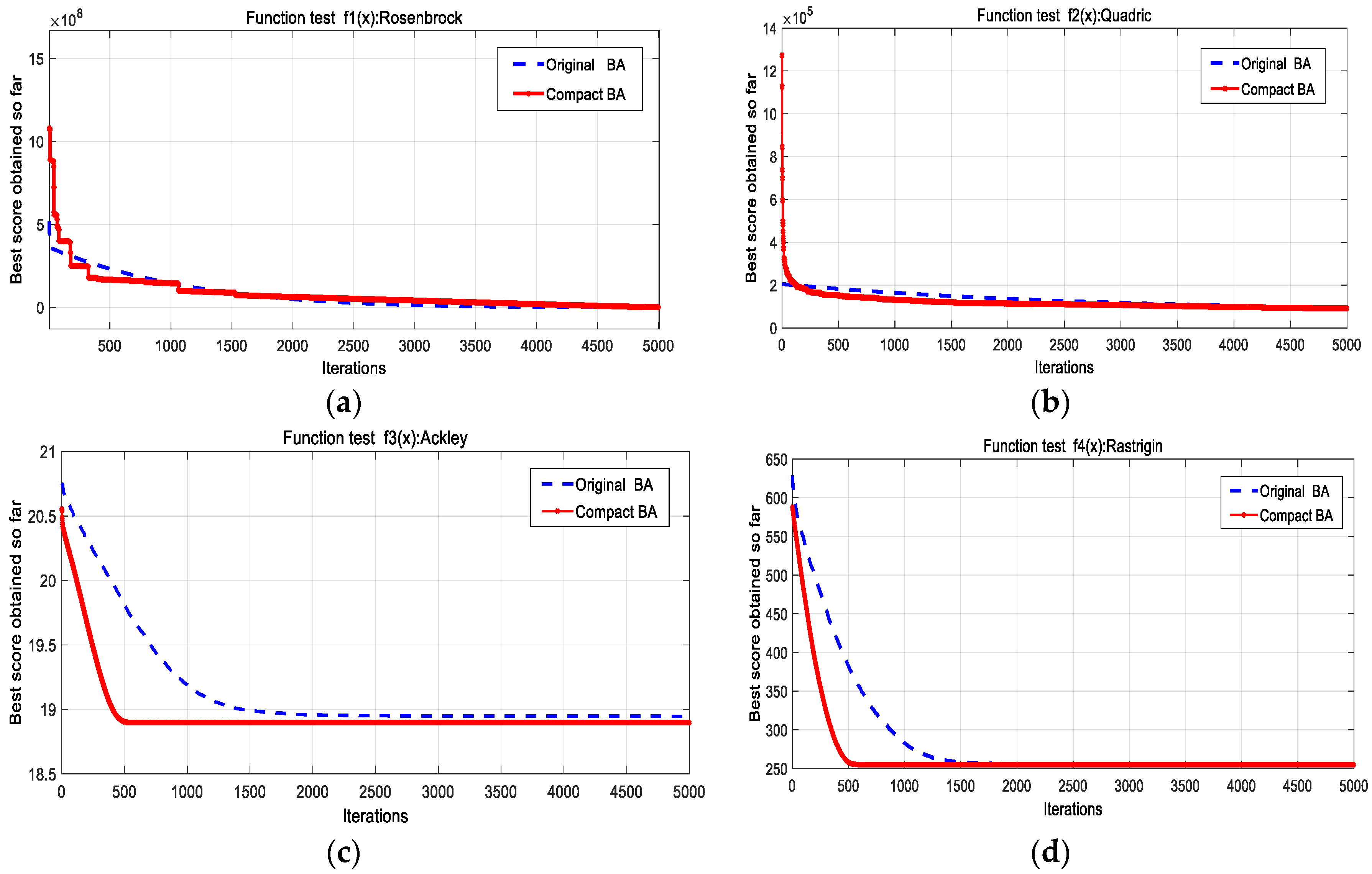
Figure 1 shows the curves of cBA and oBA with the average obtained minimum for four first test functions. It should be noted that all of these cases of test benchmark functions for cBA (red lines) are equal to or faster than oBA in convergence.

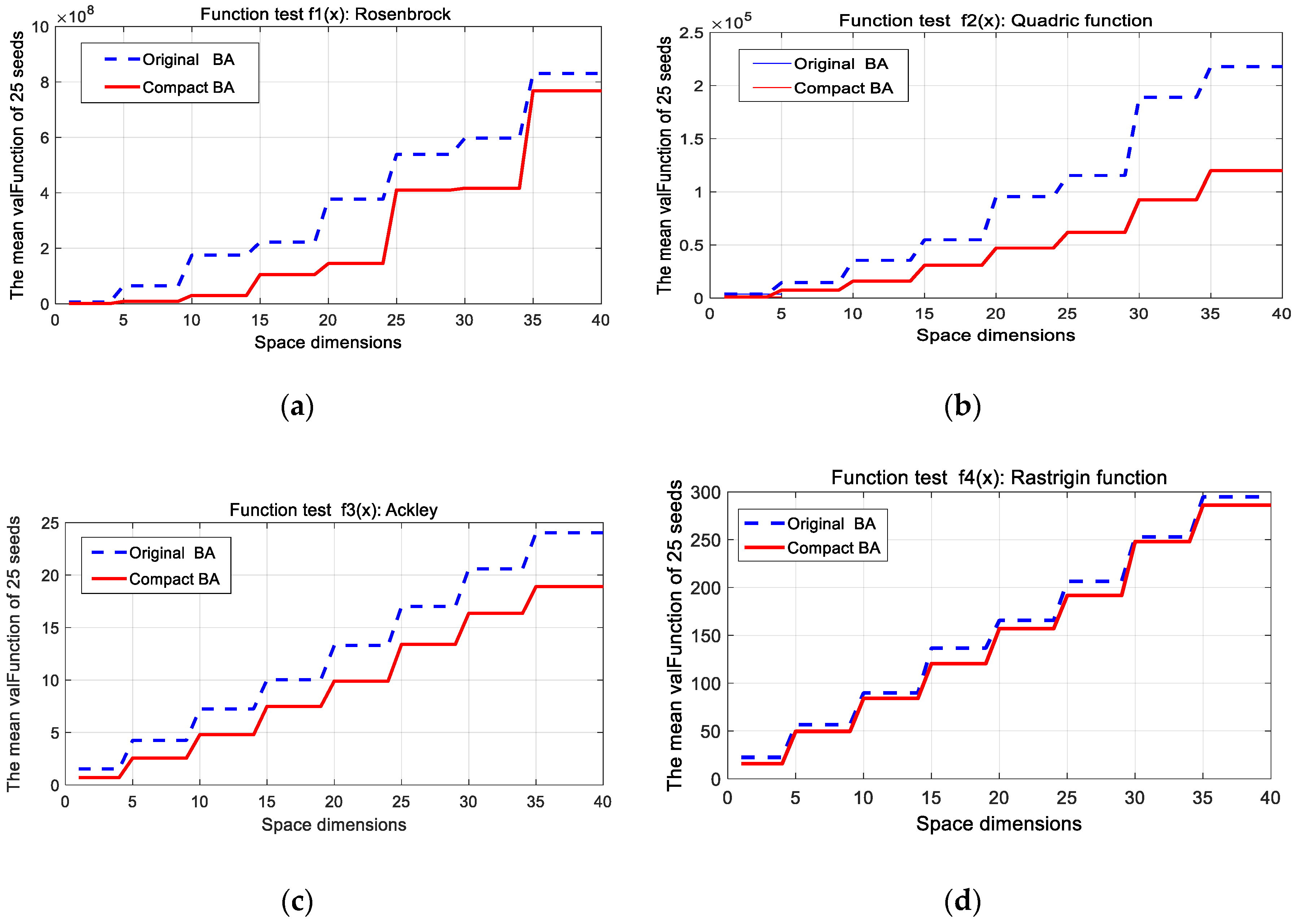
To verify the effect of population sizes on the performance of the algorithms, we used variety N for testing. Figure 2 compares the performance quality of running with different population sizes for test functions between cBA and oBA. Doubtless, most cases for testing functions in the cBA are faster than and uniform in convergence that applied for BA. The convergence of most cases of test functions for employing in cBA is not affected very much by the variety population size. Because it is a virtual population the mean value of results did not fluctuate and was more stable than that of oBA.

Table 3. Comparison of the number of variables for occupied memory slots in the cBA and oBA.

Algorithms	Number of Solutions	Occupied Slots	Used Equations
oBA	N	4 × N	(8), (9), (10), (11)
cBA	1	8	(8), (9), (10), (11), (15), (16), (17), (18)

shows the comparison of the proposed cBA with the oBA in terms of the occupied memory variables for implementing computations in running optimization. The number of variables of the two algorithms is counted for through the number of the equations used in operations optimization. Observations from Table 3 would clearly show that the number of variables of cBA use is smaller than the oBA with the same condition of computation, e.g., iterations. There are four number equations for oBA, e.g., (8)–(11) and eight equations for cBA, e.g., (8)–(11), and (15)–(18).

However, the real population or population size of oBA is N, whereas, cBA is only one. With the same number of iterations and the running time T, the stored slots of variables for oBA and cBA are 4 × T × N × iteration, and 8 × T × iteration, respectively, where T and N are the counting run time and the number of population, respectively. It is observed that the number of occupied slots in oBA is higher (N/2 times) than in cBA.

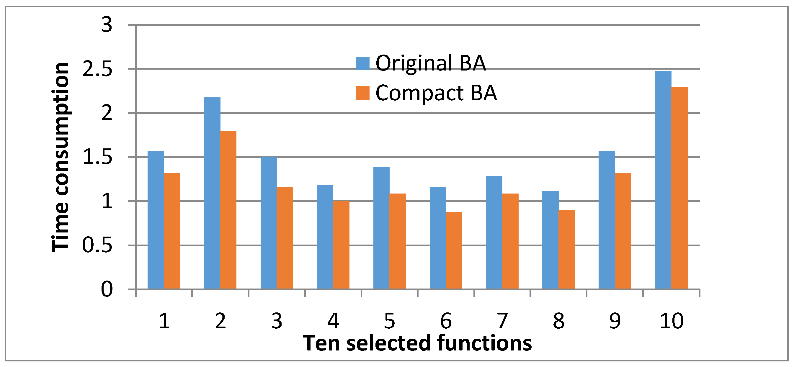
Figure 3 illustrates a comparison of executing times of the cBA with oBA over 25 runs for ten benchmark functions. Clearly, all cases of testing duties of cBA are smaller than those obtained for oBA. The average consuming time of cBA for tests is 24% faster than oBA. The reason for the rapid result is that some of the memory-stored parameters for cBA are smaller than oBA.

Table 4. Comparison of the outcomes of the proposed method with the other compact algorithms such as rcGA [39], cDE [40], and cPSO [39] for 10 test functions.

Functions	cBA	cPSO	r	cDE	r	rcGA	r
$f_1\left(x\right)$	8.97$\mathbf{\times } {\mathbf{10}}^{\mathbf{8}}$	9.20 $\times {10}^8$	+	9.20 $\times {10}^8$	+	9.00 $\times {10}^8$	~
$f_2\left(x\right)$	3.73 $\times {10}^4$	3.69$\mathbf{\times } {\mathbf{10}}^{\mathbf{4}}$	−	3.73 $\times {10}^4$	~	3.79 $\times {10}^4$	+
$f_3\left(x\right)$	1.92 $\times {10}^1$	1.91$\mathbf{\times } {\mathbf{10}}^{\mathbf{1}}$	−	1.92 $\times {10}^1$	+	1.95 $\times {10}^1$	+
$f_4\left(x\right)$	2.05$\mathbf{\times } {\mathbf{10}}^{\mathbf{2}}$	2.06 $\times {10}^2$	~	2.06 $\times {10}^2$	~	2.09 $\times {10}^2$	+
$f_5\left(x\right)$	6.11$\mathbf{\times } {\mathbf{10}}^{\mathbf{0}}$	6.12 $\times {10}^0$	+	6.23 $\times {10}^0$	+	6.23 $\times {10}^0$	+
$f_6\left(x\right)$	7.64 $\times {10}^4$	7.57 $\times {10}^4$	−	7.54$\mathbf{\times } {\mathbf{10}}^{\mathbf{4}}$	−	7.64 $\times {10}^4$	−
$f_7\left(x\right)$	1.12 $\times {10}^0$	1.19 $\times {10}^0$	+	1.13 $\times {10}^0$	+	1.10$\mathbf{\times } {\mathbf{10}}^{\mathbf{0}}$	+
$f_8\left(x\right)$	6.25$\mathbf{\times } {\mathbf{10}}^{\mathbf{3}}$	6.50 $\times {10}^3$	+	6.29 $\times {10}^3$	+	6.27 $\times {10}^3$	+
$f_9\left(x\right)$	8.75 $\times {10}^1$	1.21 $\times {10}^2$	+	7.64$\mathbf{\times } {\mathbf{10}}^{\mathbf{1}}$	−	8.75 $\times {10}^1$	~
$f_{10}\left(x\right)$	1.50 $\times {10}^0$	6.57$\mathbf{\times } {\mathbf{10}}^{\mathbf{-}1}$	−	1.81 $\times {10}^0$	+	3.18 $\times {10}^0$	+
AVG	9.07$\mathbf{\times } {\mathbf{10}}^{\mathbf{8}}$	9.21 $\times {10}^8$	+	9.20 $\times {10}^8$	+	9.10 $\times {10}^8$	+
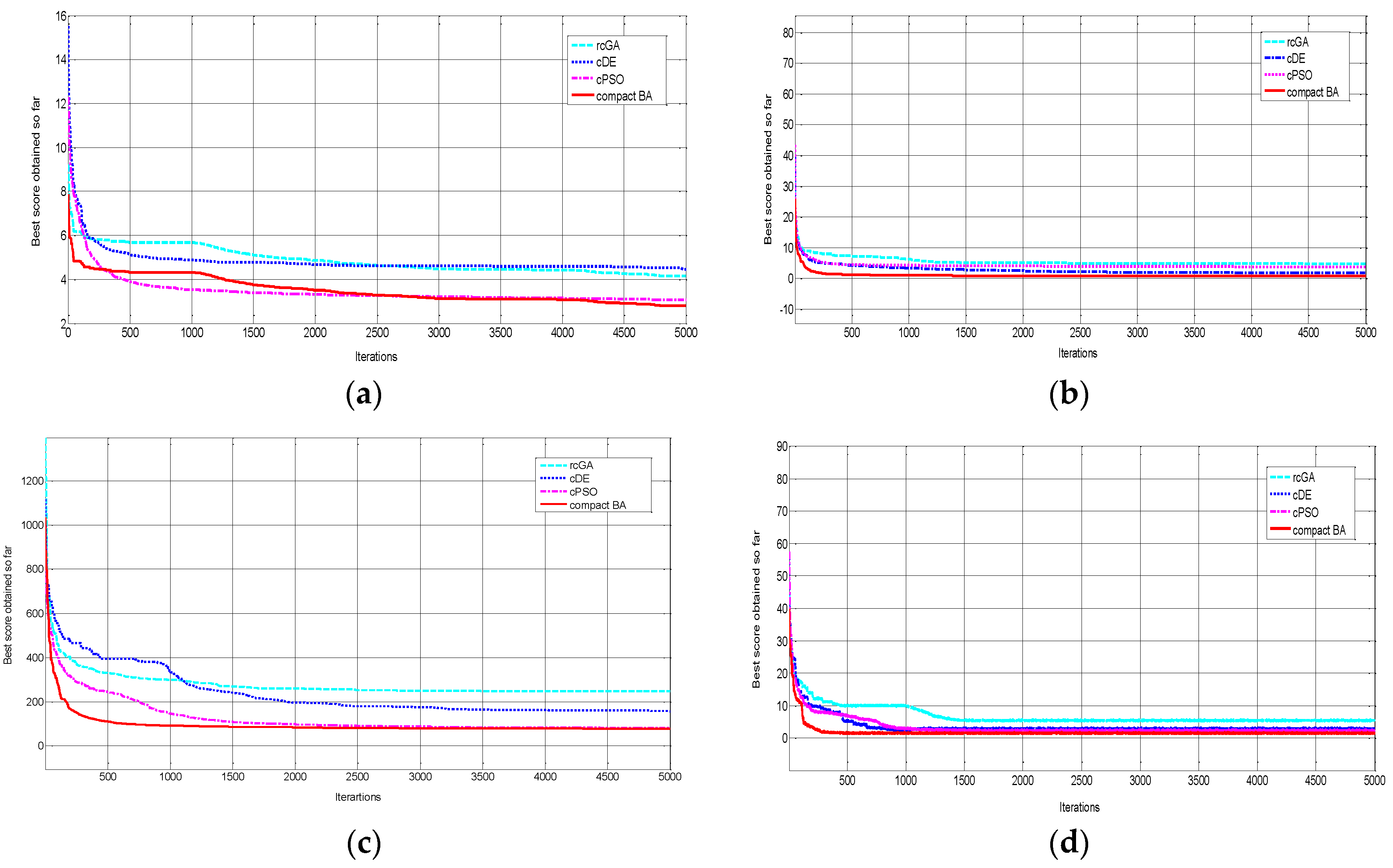
Summary	r is ‘+’, means cBA is winner	6+ 1~ 4−		7+ 2~ 2−		8+ 2~ 1−

depicts the comparison the outcomes of the proposed algorithm with the other compact algorithms such as compact Particle swarm optimization (cPSO) [39], compact Differential evolution (cDE) [40], and real compact Genetic algorithm (rcGA) [41] for 10 test functions. Apparently, cBA outperforms its competitors regarding convergence. The best results among them for each function is highlighted in rows. The performance of the compared ratio r is set for each pair of comparisons of cBA with the cPSO, cDE, and rcGA, respectively. The symbols of “+”, “−” and “~” represent “better”, “worse”, and “approximation” of the deviation of the outcomes, respectively. If the averaged outcomes obtained for 25 runs of the optimized function of cBA is better than the cPSO, cDE, and rcGA, then r is the set symbol “+”. The same method with the symbols “~” and “−” for the worse and approximation are applied to the cases, respectively. It would be seen that most of the highlighted cases of testing functions belong to the proposed cBA. Table 4 shows that the proposed approach outperforms the other methods. According to Figure 4, the curve of the cBA displays comparatively better convergence behavior on the selected test functions.

5. Experiments for Clustering in WSNs Problem

In designing and deploying sensor networks, a core demand is prolonging the lifetime of the network. A crucial factor for extending WSN lifetime is reduction of the energy consumption of the entire network. The power consumption of WSNs is affected directly by the clustering criterion problem. Furthermore, the cause of the hot spot problem in a WSN with multi-hop communications is unbalanced energy consumption. The higher energy consumption nodes are closer to the base station (BS) because of the heavy traffic flows. In this section, cBA is applied to optimize the design of the WSN by balancing the load between the CHs. We utilize adjustable parameter of loudness of BA for supporting and preventing unbalanced energy consumption. The loudness Ai of the BA can vary and alter responds to distances in clustering criterion for unequal clustering in WSN. The optimized total communication distances from the cluster members to the CHs and the CHs to the BS in the WSNs can provide the energy savings [42]. The sequence of experimental steps consists of modeling objective function, setting up a mapping solution model, describing proper agent representation, optimizing CHs, and comparing results.

5.1. Objective Function

The objective function is modelled with not only minimizing the optimized total communication distances from the cluster members to the CHs and the CHs to the BS but also by balancing energy consumption between the CHs and group members. Referring to Equation (3), the CHs is selected based on energy residual.

$$f_1\left(x_i\right)= \frac{{\sum }_{i=1}^N{E}_i}{{\sum }_{k=1}^k{E}_{C{H}_k}}$$

(19)

In Equation (6), we use only the optimizable component that was independent of parameters related to the microcontroller and the supply voltage distances. Consequently, E_frame is the most affected factor of the energy loss depending on the distance of the clustering in WSN. Therefore, the consuming energy of the network is based on the distances in the clusters. Sensor nodes are clustered by using entire distances, namely $E_{distance}$, where k is the given clusters.

$$E_{distance}={\displaystyle \sum }_{j=1}^k{\displaystyle \sum }_{i=1}^{n_j}\left(d_{ij}^2+\frac{D_j^2}{n_j}\right)$$

(20)

Another factor that affected the fitness function is calculated as follows:

$$f_2\left(x_i\right)=min\left({\displaystyle \sum }_{j=1}^k{\displaystyle \sum }_{i=1}^{n_j}\left(d_{ij}^2+\frac{D_j^2}{n_j}\right)\right)$$

(21)

where ${\sum }_{j=1}^k{n}_j+k=N$ is the number of nodes in a network, $d$ and $D$ are the distances of member nodes to the CH and the CHs to the BS, respectively.

Modelling for objective function suggests dense clusters with set of nodes which have sufficient energy to perform the CH tasks. The objective function for equal clustering in WSN is defined as follows:

$$Minimize F=\theta \times f_1\left(x_i\right)+\left(1-\theta \right)\times f_2\left(x_i\right)$$

(22)

where $\theta$ is weight of the objective function. The vector of bats x is represented by mapping from the distances of $d_{ij}$ with the indexed $D_j$. Both types of distances are considered the intra-cluster distance and the distance between the CHs and the BS. The intra-cluster distances are distances of member nodes and its CH.

5.2. Model Solution Representation

A WSN is assumed to be a graph G with n nodes randomly distributed in the desired area. There are N nodes (N is set to 100, 200, …) in a network spread out in a distributed two-dimensional space of $\left(0:M,0:M\right),$ where M equals 100, 200. The nodes of the WSN circulate in a two-dimensional area and are deployed as follows: (1) a model solution is constructed with spatial coordinates of nodes that can obtain distances to the BS and attribute links between the nodes, (2) clusters are figured out randomly with k clusters, and (3) the distance of the cluster member to the CH and the CHs to the BS are calculated for optimization of the network layout.

Table 5. A sample of representative positions of the sensor nodes.

Index	Nodei	1	2	3	4	5	6	7	8	9	10	11	..	n
x	05	55	85	101	72	60	45	40	50	75	45	20	..	10
y	01	5	10	30	15	20	45	60	85	90	95	80	..	80

shows an example of the position of randomly distributed nodes in two-dimensional coordinates of a network zone. Each node can communicate with others by r transmission ranging. Node i can receive the signal of node j if node i is in the transmission range $r$ of node j.

Table 6. The attribution of existing cluster heads (CHs) if flag = 1 and node is set to cluster head (CH). Otherwise node is set to member node (SN).

Index	Nodei	1	2	3	4	5	6	7	8	9	10	11	12	13	..	n
Cluster head		0	0	0	0	1	0	0	0	0	0	0	0	1	..	0

indicates the attribution of the existing CHs in the sensor networks.

In the following experiment, we consider two scenarios of equal clustering and unequal clustering in a WSN to create an optimization network. The equal clustering has cluster radii which are the same size. However, the group size of unequal clustering close to the BS is smaller than those that are farther from the BS. The uneven cluster sizes occur because the traffic relay load of the CHs near the base station is heavier than the CHs farther away from the BS.

5.3. Equal Clustering Formation

The optimization problem is dealt with by minimizing the objective function in Equation (22). The initial setting for the oBA and the cBA is the same condition in the WSN (denoted as oBA-WSN and cBA-WSN), e.g., a maximum iteration is set to 2000, the number of runs is set to 25. (Readers refer to parameters setting of the loudness, frequencies, and virtual population in Section 4). The initial energy parameters of the sensor net are flowing: l = 1024 bit, E_j = 0:5 J, E_mp = 0:0013 pJ/bit/m⁴, E_fs = 10 pJ/bit/m², E_DA = 5 nJ/bit/signal, E_elec = 50 nJ/bit [31]. The experimental results of the proposed cBA are compared with the cases of PSO: the time-varying inertia weight (PSO-TVIW), and time-varying acceleration coefficients (PSO-TVAC) in [43] and the oBA [44] with respect to solution quality and time running. The result averages the outcomes from all runs.

Table 7. The comparison of averaged outcomes and computation time of cBA-WSN with other methods, e.g., oBA-WSN [44], PSO-TVAC [43] and PSO-TVIW [43] for equal clustering formation.

Methods	Pop. Size	Iterations/a Run	Min	Max	Mean	Standard Deviation	Running Time (m)
$\mathrm{PSO}-\mathrm{TVAC}$ [43]	20	2000	5.72 $\times {10}^1$	8.41 $\times {10}^2$	2.57 $\times {10}^2$	2.87 $\times {10}^2$	3.01 $\times {10}^0$
$\mathrm{PSO}-\mathrm{TVIW}$ [43]	20	2000	6.80 $\times {10}^1$	6.35 $\times {10}^2$	2.25 $\times {10}^2$	2.83 $\times {10}^2$	3.10 $\times {10}^0$
oBA-WSN [44]	20	2000	6.93 $\times {10}^1$	7.57 $\times {10}^2$	2.03 $\times {10}^2$	2.69 $\times {10}^2$	3.26 $\times {10}^0$
The proposed cBA-WSN	1	2000	$\mathbf{5.65}\mathbf{\times }{\mathbf{10}}^{\mathbf{1}}$	$\mathbf{7.65}\mathbf{\times }{\mathbf{10}}^{\mathbf{2}}$	$\mathbf{2.01}\mathbf{\times }{\mathbf{10}}^{\mathbf{2}}$	$\mathbf{2.32}\mathbf{\times }{\mathbf{10}}^{\mathbf{2}}$	$\mathbf{2.04}\mathbf{\times }{\mathbf{10}}^{\mathbf{0}}$

compares the performance quality and running time for optimizing the clustering formation in WSNs for four methods of the $\mathrm{cBA}-\mathrm{WSN}$, $\mathrm{PSOTVAC}-\mathrm{WSN}$, $\mathrm{PSOTVIW}-\mathrm{WSN}$, and the $\mathrm{oBA}-\mathrm{WSN}$. Clearly, the average value of cBA for the objective function are faster than those obtained by other approaches of PSO. The applied cBA for optimizing the clustering formation is not as different as convergence using oBA. But, the total time consumption of the cBA method is fastest at only 2.445 min taken because the working variable memory is smallest.

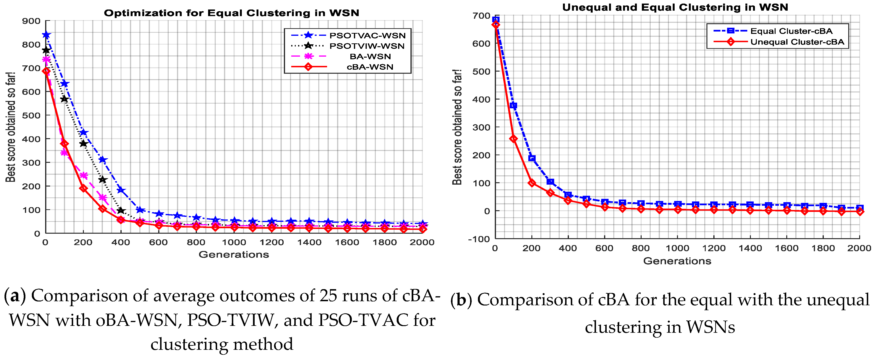
Figure 5a indicates four curves of the $\mathrm{cBA}-\mathrm{WSN}$, $\mathrm{oBA}-\mathrm{WSN}$, $\mathrm{PSOTVIW}-\mathrm{WSN}$ and $\mathrm{PSOTVAC}-\mathrm{WSN}$ methods for clustering formation for WSN. It is evident that cBA-WSN is as good as BA-WSN and faster than those of $\mathrm{PSOTVIW}-\mathrm{WSN}$ and $\mathrm{PSOTVAC}-\mathrm{WSN}$ methods in convergence.

5.4. Unequal Clustering Formation

This unequal clustering scenario is studied to deal with the hot spot problem in WSN. The partitioned clusters in the network of uneven clustering have different sizes. The groups close to the BS are smaller than those clusters far from the BS. The clusters closer to the BS are the hotter clusters because the traffic relay load of the cluster heads near the BS is heavier than those CHs farther away from the BS [45]. To avoid this hot spot problem, we determine that the adjustable parameters are not only related to the objective function but also related to the optimization algorithm. For the objective function of constructing unequal clusters, each CH needs to adjust its equal cluster distances:

$$D_j=D_j\times R_c$$

(23)

where $D_j$ is the distance from node CH_j to the BS, and $R_c$ is the ratio adjusting parameter. The calculation for $R_c$ is defined as follows:

$$R_c=\left[1-\alpha \frac{d_{max}-D_j}{d_{max}-d_{min}}-\beta \left(1-\frac{E_r}{E_{max}}\right)\right]\times R_{max}$$

(24)

where $d_{max}$ and $d_{min}$ are the maximum and minimum distance of the CHs in the network to the BS, $R_{max}$ is the maximum value of competition radius, α is a weighted factor whose value is in (0, 1), and $E_r$ is the residual energy of CH_j. Clustering optimized formation is done by performing the optimal objective function in Equation (22) with the assistant of different distances Equations (23) and (24).

Figure 5b compares two performance qualities in two scenarios of equal clustering and hot spot problems. Visibly, the average fitness values of the cBA method with a hot spot issue in the case of adjusting cluster size for the unequal clustering formation is faster than the regular case in convergence.

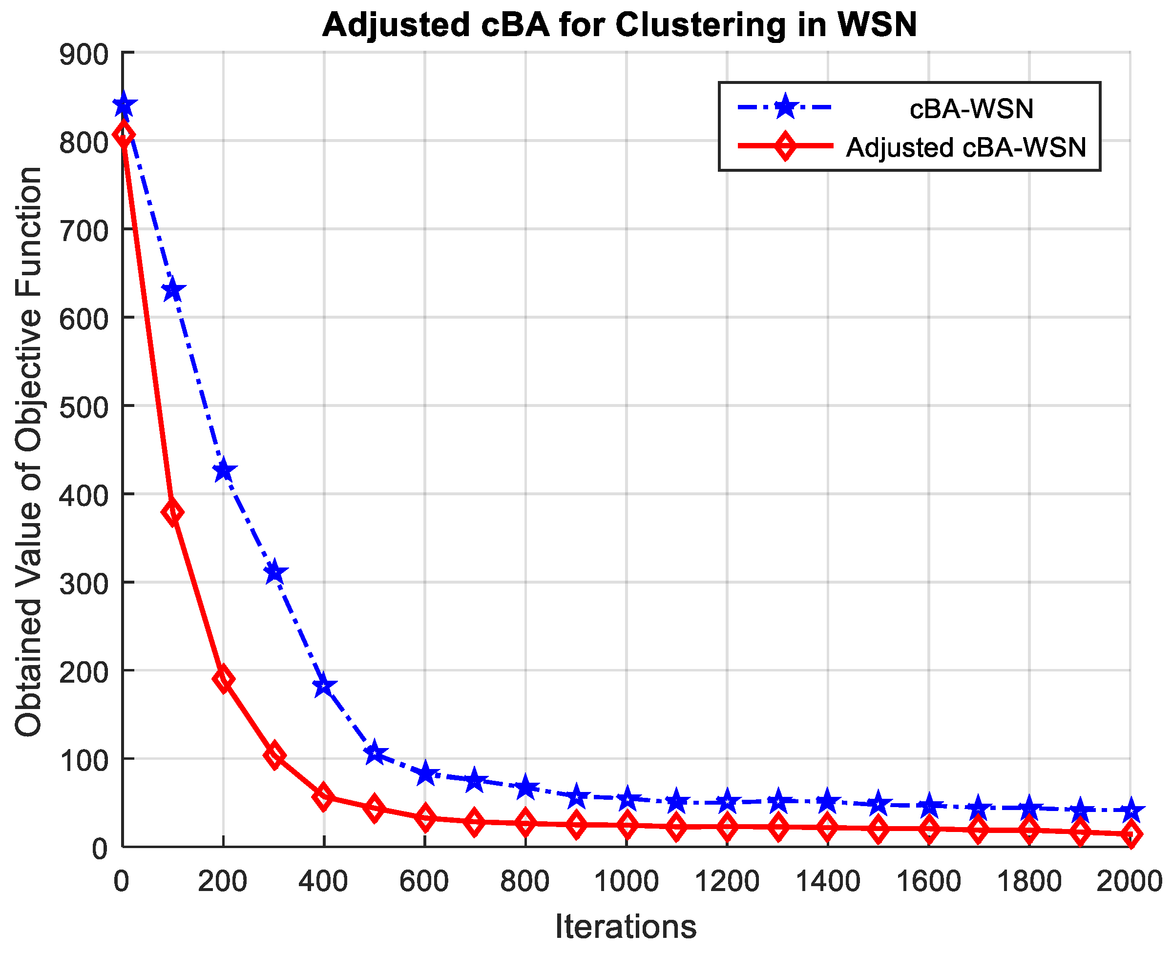
For the optimization algorithm, we assigned the variable of loudness Ai for BA as in Equation (12) to correspond to the radius of the changing cluster size by bias iteration. We expressed mathematically the time-varying loudness of the BA as follows:

$$A_i^0=(A_{max}-A_{min})\times \frac{\left(MaxIteration-Iter\right)}{MaxIteration}+A_{min}$$

(25)

where $MaxIteration$ is the number of the maximum iteration; $Iter$ is the current time steps, and $A_{max}, A_{min}$ are constants set to 0.5 and 0.25, respectively. The time varying loudness is mathematically represented in Equation (25) for cBA with a hot spot problem in WSN.

Figure 6 compares the performance qualities in two cases of the selected parameter of the loudness for cBA with an adjusted cluster size with no selected altered loudness setting. Visibly, the average fitness values for the cBA method in the case of adjusting Ai for the unequal clustering formation is better than the regular case in convergence to remove the hot spot problem.

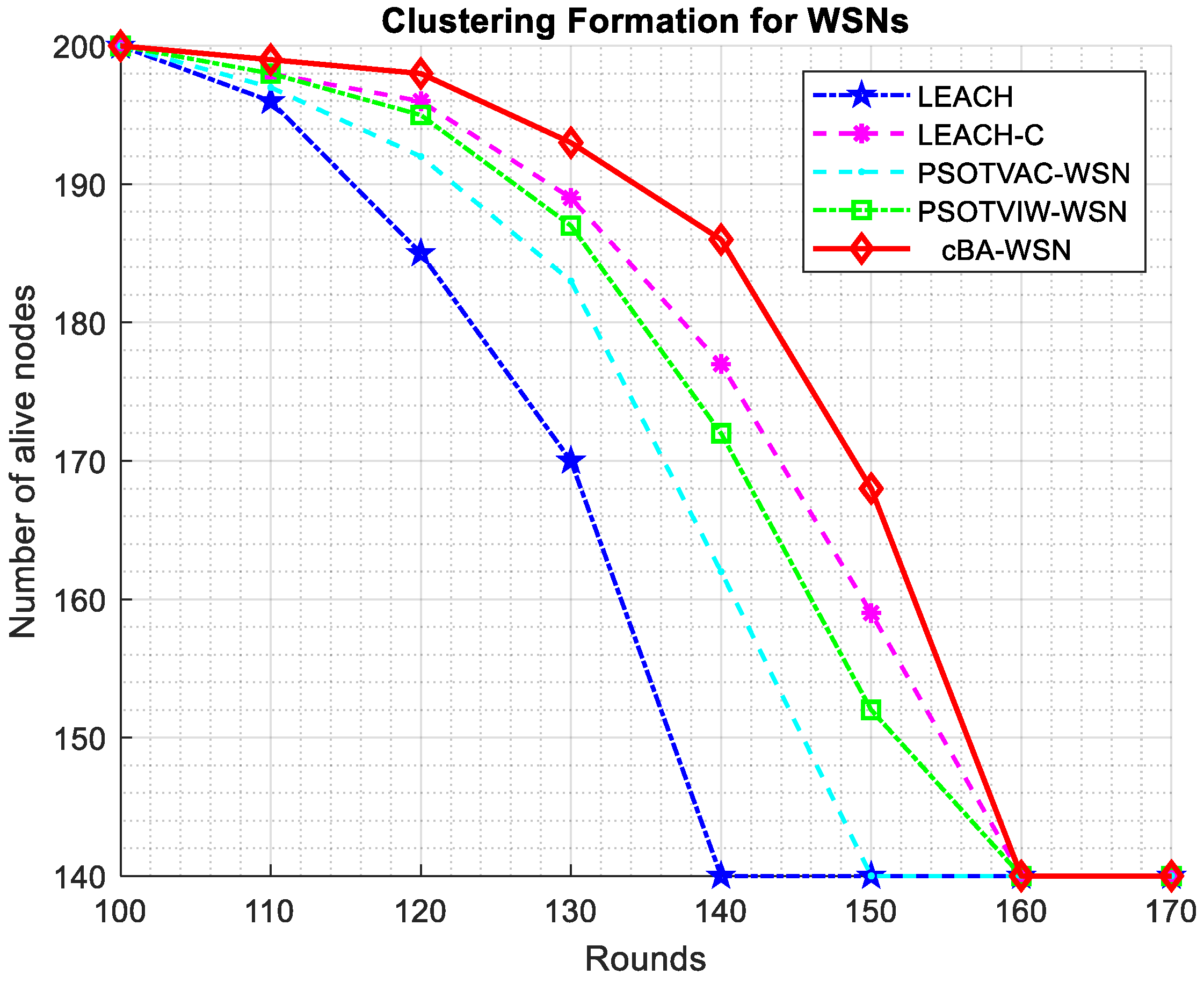
Figure 7 shows a comparison of the advanced cBA-WSN with other methods, e.g., PSO-TVAC, PSO-TVIW, the low-energy adaptive clustering hierarchy (LEACH) [22], and LEACH-centralized (LEACH-C) [23] approaches regarding the number of nodes alive. LEACH is a clustering protocol that selects sensor nodes randomly as CHs based on probability as a “threshold” parameter. LEACH-C is another version based on LEACH with a base station (BS) and uses a specific method to select the CH and divide the nodes to clusters which can offer more optimization, and therefore it means the lifetime of the network is longer than LEACH. On the basis of observations, it is clear that the number of alive nodes of the proposed cBA-WSN is the longest. This means that the results of the proposed cBA-WSN for the testing functions and clustering problem in WSN is better than the other methods in the comparisons.

6. Conclusions

This paper presented a new optimization algorithm using the compact bat algorithm (cBA) for the uneven clustering problem in wireless sensor networks (WSN). A probabilistic model was used to generate a new candidate solution in space search using the cBA which has been promising so far. The candidate solution was found by studying explicit probabilistic models of promising existing solutions and sampling the built models. The probability density functions (PDF) and cumulative distribution functions (CDF) thoroughly are used to construct the operations of selecting and optimizing behaviors. The probabilistic model is used as a valid alternative optimization strategy for available devices with even limited hardware sources. Experimental results demonstrate that the proposed algorithm achieves the effective way of using limited memory devices, and provides competitive results.

References

- Yang, X.S. A New Metaheuristic Bat-Inspired Algorithm. In Studies in Computational Intelligence; González, J., Pelta, D., Cruz, C., Terrazas, G., Krasnogor, N., Eds.; Springer: Heidelberg, Germany, 2010; Volume 284, pp. 65–74. [Google Scholar]
- Dao, T.K.; Pan, J.S.; Nguyen, T.T.; Chu, S.C.; Shieh, C.S. Compact Bat Algorithm. In Advances in Intelligent Systems and Computing; Pan, J.-S., Snasel, V., Corchado, E.S., Abraham, A., Wang, S.-L., Eds.; Springer International Publishing: Heidelberg, Germany, 2014; Volume 298, pp. 57–68. [Google Scholar]
- Yang, X. Bat Algorithm: Literature Review and Applications. Int. J. Bio-Inspired Comput. 2013, 5, 1–10. [Google Scholar] [CrossRef]
- Dao, T.; Pan, T.; Nguyen, T.; Chu, S. Evolved Bat Algorithm for Solving the Economic Load Dispatch Problem. Adv. Intell. Syst. Comput. 2015, 329, 109–119. [Google Scholar]
- Tsai, P.W.; Pan, J.S.; Liao, B.Y.; Tsai, M.J.; Istanda, V. Bat algorithm inspired algorithm for solving numerical optimization problems. Appl. Mech. Mater. 2012, 148, 134–137. [Google Scholar] [CrossRef]
- Nguyen, T.-T.; Pan, J.-S.; Dao, T.-K.; Kuo, M.-Y.; Horng, M.-F. Hybrid Bat Algorithm with Artificial Bee Colony; Springer: Heidelberg, Germany, 2014; Volume 298. [Google Scholar]
- Nakamura, R.Y.M.; Pereira, L.A.M.; Rodrigues, D.; Costa, K.A.P.; Papa, J.P.; Yang, X.-S. Binary bat Algorithm for Feature Selection. In Swarm Intelligence and Bio-Inspired Computation; Elsevier: Amsterdam, The Netherlands, 2013; pp. 225–237. [Google Scholar]
- Mirjalili, S.; Mirjalili, S.M.; Yang, X.-S. Binary bat algorithm. Neural Comput. Appl. 2014, 25, 663–681. [Google Scholar] [CrossRef]
- Kang, M.; Kim, J.; Kim, J.-M. Reliable fault diagnosis for incipient low-speed bearings using fault feature analysis based on a binary bat algorithm. Inf. Sci. 2015, 294, 423–438. [Google Scholar] [CrossRef] [Green Version]
- Zhao, D.; He, Y. Chaotic binary bat algorithm for analog test point selection. Analog Integr. Circuits Signal Process. 2015, 84, 201–214. [Google Scholar]
- Rizk-Allah, R.M.; Hassanien, A.E. New binary bat algorithm for solving 0–1 knapsack problem. Complex Intell. Syst. 2018, 4, 31–53. [Google Scholar] [CrossRef]
- Dao, T.-K.; Pan, T.-S.; Nguyen, T.-T.; Pan, J.-S. Parallel bat algorithm for optimizing makespan in job shop scheduling problems. J. Intell. Manuf. 2018, 29, 451–462. [Google Scholar] [CrossRef]
- Luo, Q.; Zhou, Y.; Xie, J.; Ma, M.; Li, L. Discrete bat algorithm for optimal problem of permutation flow shop scheduling. Sci. World J. 2014, 2014, 15. [Google Scholar] [CrossRef] [PubMed]
- Osaba, E.; Yang, X.-S.; Diaz, F.; Lopez-Garcia, P.; Carballedo, R. An improved discrete bat algorithm for symmetric and asymmetric traveling salesman problems. Eng. Appl. Artif. Intell. 2016, 48, 59–71. [Google Scholar] [CrossRef]
- Estrin, D.; Heidemann, J.; Kumar, S.; Rey, M. Next Century Challenges: Scalable Coordination in Sensor Networks. In Proceedings of the 5th annual ACM/IEEE International Conference on Mobile Computing and Networking, Seattle, WA, USA, 18–19 August 1999; Volume 4, pp. 263–270. [Google Scholar]
- Nguyen, T.-T.; Dao, T.-K.; Horng, M.-F.; Shieh, C.-S. An Energy-based Cluster Head Selection Algorithm to Support Long-lifetime in Wireless Sensor Networks. J. Netw. Intell. 2016, 1, 23–37. [Google Scholar]
- Liu, W.; Vijayanagar, K.R.; Kim, J. Low-complexity distributed multiple description coding for wireless video sensor networks. IET Wirel. Sens. Syst. 2013, 3, 205–215. [Google Scholar] [CrossRef]
- Almalkawi, I.T.; Zapata, M.G.; Al-Karaki, J.N.; Morillo-Pozo, J. Wireless multimedia sensor networks: Current trends and future directions. Sensors 2010, 10, 6662–6717. [Google Scholar] [CrossRef] [PubMed]
- Djedjiga, A.A.; Abdeldjalil, O. Monitoring crack growth using thermography. C. R. Mec. 2008, 336, 677–683. [Google Scholar]
- Broday, D.M. Wireless distributed environmental sensor networks for air pollution measurement—The promise and the current reality. Sensors 2017, 17, 2263. [Google Scholar] [CrossRef] [PubMed]
- Meriem, D.; Abdeldjalil, O.; Hadj, B.; Adrian, B.; Denis, K. Discrete Wavelet for Multifractal Texture Classification: Application to Medical Ultrasound Imaging. In Proceedings of the 2010 IEEE International Conference on Image Processing, Hong Kong, China, 26–29 September 2010; pp. 637–640. [Google Scholar]
- Medina-García, J.; Sánchez-Rodríguez, T.; Galán, J.; Delgado, A.; Gómez-Bravo, F.; Jiménez, R. A wireless sensor system for real-time monitoring and fault detection of motor arrays. Sensors 2017, 17, 469. [Google Scholar] [CrossRef]
- Fernandez-Lozano, J.J.; Martín-Guzmán, M.; Martín-Ávila, J.; García-Cerezo, A. A wireless sensor network for urban traffic characterization and trend monitoring. Sensors 2015, 15, 26143–26169. [Google Scholar] [CrossRef]
- Garcia-Sanchez, A.-J.; Garcia-Sanchez, F.; Garcia-Haro, J. Wireless sensor network deployment for integrating video-surveillance and data-monitoring in precision agriculture over distributed crops. Comput. Electron. Agric. 2011, 75, 288–303. [Google Scholar] [CrossRef]
- Akyildiz, I.; Su, W.; Sankarasubramaniam, Y.; Cayirci, E. Wireless sensor networks: A survey. Comput. Netw. 2002, 38, 393–422. [Google Scholar] [CrossRef]
- García-hernández, C.F.; Ibargüengoytia-gonzález, P.H.; García-hernández, J.; Pérez-díaz, J.a. Wireless Sensor Networks and Applications: A Survey. J. Comput. Sci. 2007, 7, 264–273. [Google Scholar]
- Pan, J.-S.; Kong, L.; Sung, T.-W.; Tsai, P.-W.; Snášel, V. A Clustering Scheme for Wireless Sensor Networks Based on Genetic Algorithm and Dominating Set. J. Int. Technol. 2018, 19, 1111–1118. [Google Scholar]
- Wolpert, D.H.; Macready, W.G. No free lunch theorems for optimization. IEEE Trans. Evolut. Comput. 1997, 1, 67–82. [Google Scholar] [CrossRef] [Green Version]
- Abbasi, A.A.; Younis, M. A survey on clustering algorithms for wireless sensor networks. Comput. Commun. 2007, 30, 2826–2841. [Google Scholar] [CrossRef]
- Xia, H.; Zhang, R.H.; Yu, J.; Pan, Z.K. Energy-Efficient Routing Algorithm Based on Unequal Clustering and Connected Graph in Wireless Sensor Networks. Int. J. Wirel. Inf. Netw. 2016, 23, 141–150. [Google Scholar] [CrossRef]
- Heinzelman, W.B.; Chandrakasan, A.P.; Balakrishnan, H. An application-specific protocol architecture for wireless microsensor networks. IEEE Trans. Wirel. Commun. 2002, 1, 660–670. [Google Scholar] [CrossRef] [Green Version]
- Heinzelman, W.B. Application-Specific Protocol Architectures for Wireless Networks; Massachusetts Institute of Technology: Cambridge, MA, USA, 2000. [Google Scholar]
- Nguyen, T.-T.; Shieh, C.-S.; Dao, T.-K.; Wu, J.-S.; Hu, W.-C. Prolonging of the Network Lifetime of WSN Using Fuzzy Clustering Topology. In Proceedings of the 2013 2nd International Conference on Robot, Vision and Signal Processing, RVSP, Kitakyushu, Japan, 10–12 December 2013. [Google Scholar]
- Billingsley, P. Probability and Measure, 3th ed.; Wiley: Hoboken, NJ, USA, 1995. [Google Scholar]
- Larranaga, P.; Lozano, J.A. Estimation of Distribution Algorithms—A New Tool for Evolutionary Computation; Springer Science & Business Media: Heidelberg, Germany, 2002; Volume 2. [Google Scholar]
- Bronshtein, I.N.; Semendyayev, K.A.; Musiol, G.; Mühlig, H. Handbook of Mathematics, 6th ed.; Van Nostrand Reinhold: New York, NY, USA, 2015. [Google Scholar]
- Ghosh, S.K. Handbook of Mathematics; No. 3; Van Nostrand Reinhold: New York, NY, USA, 1989; Volume 18. [Google Scholar]
- Yao, X.; Liu, Y.; Lin, G. Evolutionary programming made faster. IEEE Trans. Evol. Comput. 1999, 3, 82–102. [Google Scholar] [Green Version]
- Neri, F.; Mininno, E.; Iacca, G. Compact particle swarm optimization. Inf. Sci. 2013, 239, 96–121. [Google Scholar] [CrossRef]
- Mininno, E.; Neri, F.; Cupertino, F.; Naso, D. Compact differential evolution. IEEE Trans. Evol. Comput. 2011, 15, 32–54. [Google Scholar] [CrossRef]
- Harik, G.R.; Lobo, F.G.; Goldberg, D.E. The compact genetic algorithm. IEEE Trans. Evol. Comput. 1999, 3, 287–297. [Google Scholar] [CrossRef]
- Akyildiz, I.F.; Su, W.; Sankarasubramaniam, Y.; Cayirci, E. A survey on sensor networks. IEEE Commun. Mag. 2002, 40, 102–105. [Google Scholar] [CrossRef]
- Ratnaweera, A.; Halgamuge, S.K.; Watson, H.C. Self-organizing hierarchical particle swarm optimizer with time-varying acceleration coefficients. IEEE Trans. Evol. Comput. 2004, 8, 240–255. [Google Scholar] [CrossRef] [Green Version]
- Nguyen, T.-T.; Shieh, C.-S.; Horng, M.-F.; Ngo, T.-G.; Dao, T.-K. Unequal Clustering Formation Based on Bat Algorithm forWireless Sensor Networks. In Knowledge and Systems Engineering: Proceedings of the Sixth International Conference KSE 2014; Nguyen, V.-H., Le, A.-C., Huynh, V.-N., Eds.; Springer International Publishing: Cham, Switzerland, 2015; pp. 667–678. [Google Scholar]
- Pan, J.-S.; Kong, L.; Sung, T.-W.; Tsai, P.-W.; Snášel, V. α-Fraction First Strategy for Hierarchical Model in Wireless Sensor Networks. J. Internet Technol. 2018, 19, 1717–1726. [Google Scholar]
Figure 1.
Convergence comparison of two algorithms of cBA and oBA for four first test functions. (a): Rosenbrock function; (b): Quadric function; (c): Ackley function; (d): Rastrigin function.
Figure 2.
Comparison of two curves with affected variety of the population size in BA and compact BA for four first test functions. (a): Rosenbrock function; (b): Quadric function; (c): Ackley function; (d): Rastrigin function.
Figure 3.
Comparison of running times of cBA with cBA for ten test functions.
Figure 4.
Comparison of four compact algorithms of rcGA, cDE, cPSO, and cBA for the selected testing functions: (a) is f1, (b) is f2, (c) is f5 and (d) is f7.
Figure 5.
Two scenarios of clustering and unequal clustering methods in WSNs.
Figure 6.
Comparison of converging curves of the cBA-WSN (with adjusted cluster size for BAs with altered loudness) and the cBA-WSN (with no adjusted).
Figure 7.
Comparison of advanced cBA-WSN for the number of nodes alive for a WSNs with PSO-TVAC, PSO-TVIW, LEACH, and LEACH-C approaches.