Can Decomposition Approaches Always Enhance Soft Computing Models? Predicting the Dissolved Oxygen Concentration in the St. Johns River, Florida

 , ,
, ,  , ,
, ,
Abstract
:1. Introduction
2. Materials and Methods
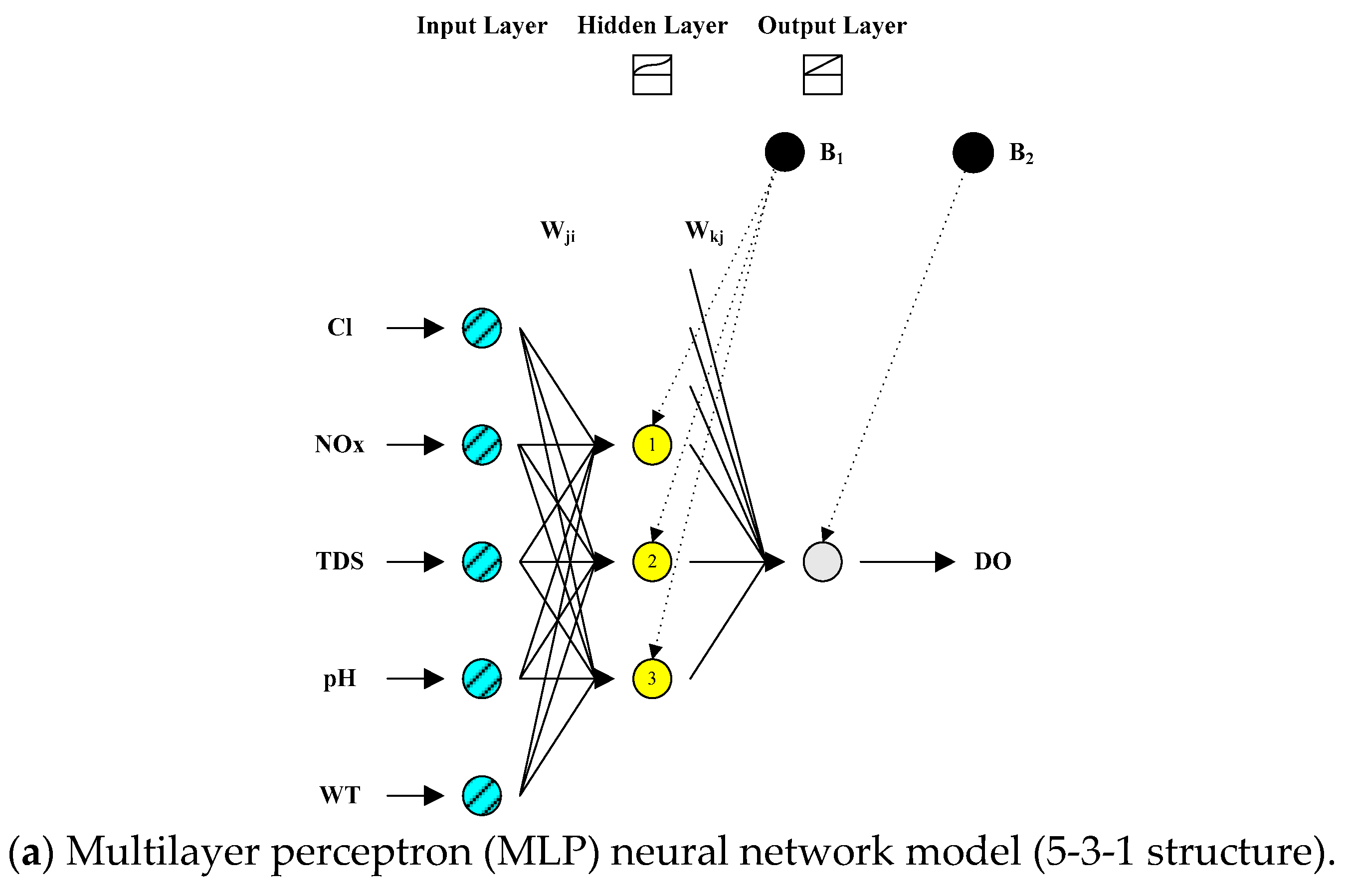
2.1. Multilayer Perceptron (MLP) Neural Network Model
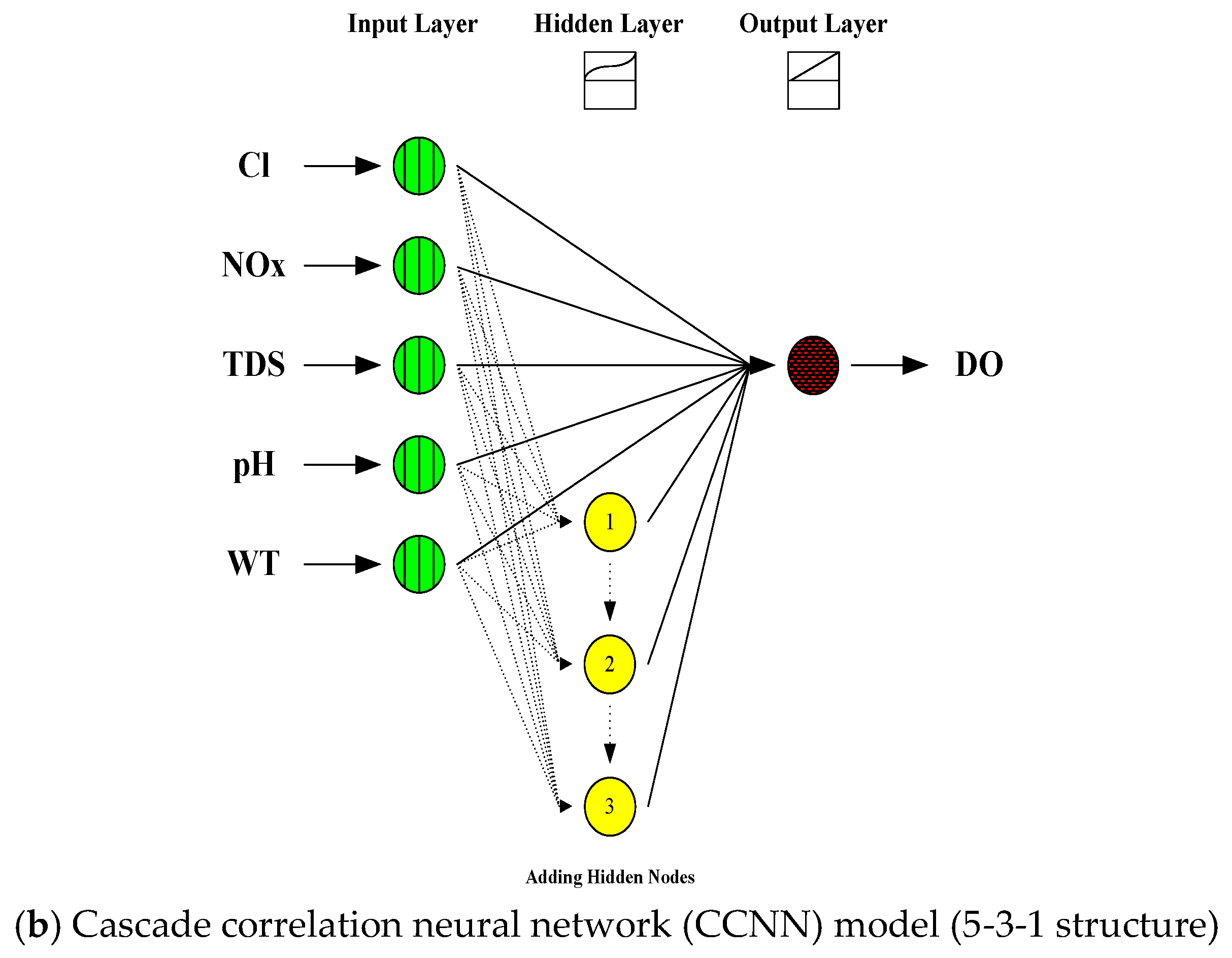
2.2. Cascade Correlation Neural Network (CCNN) Model
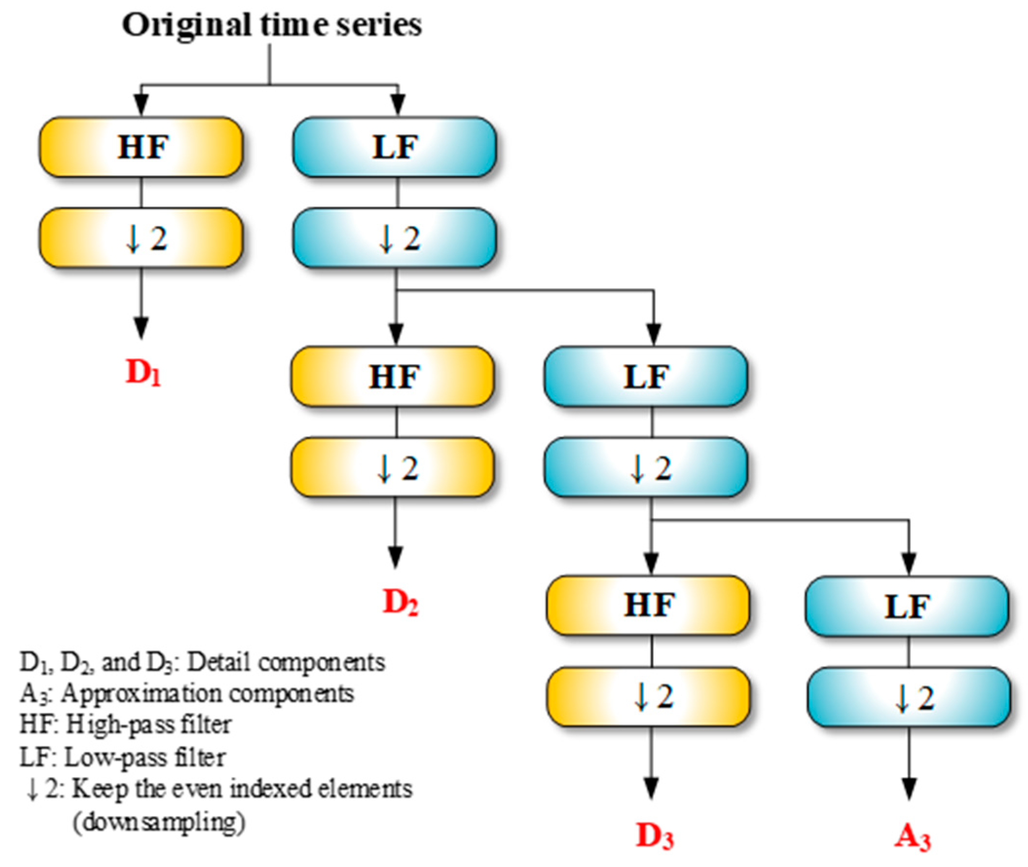
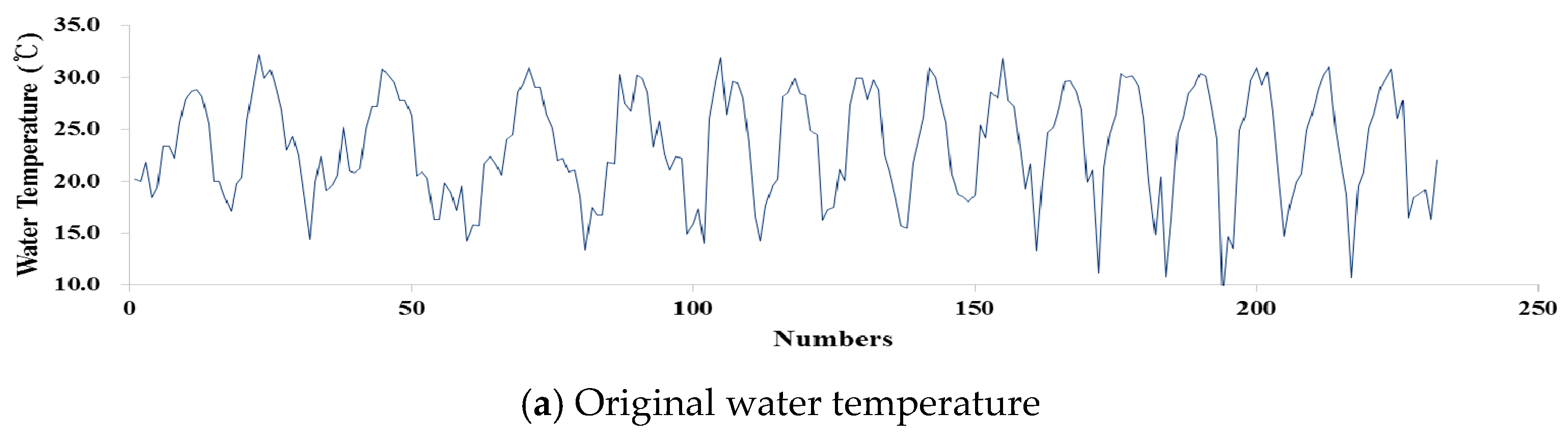
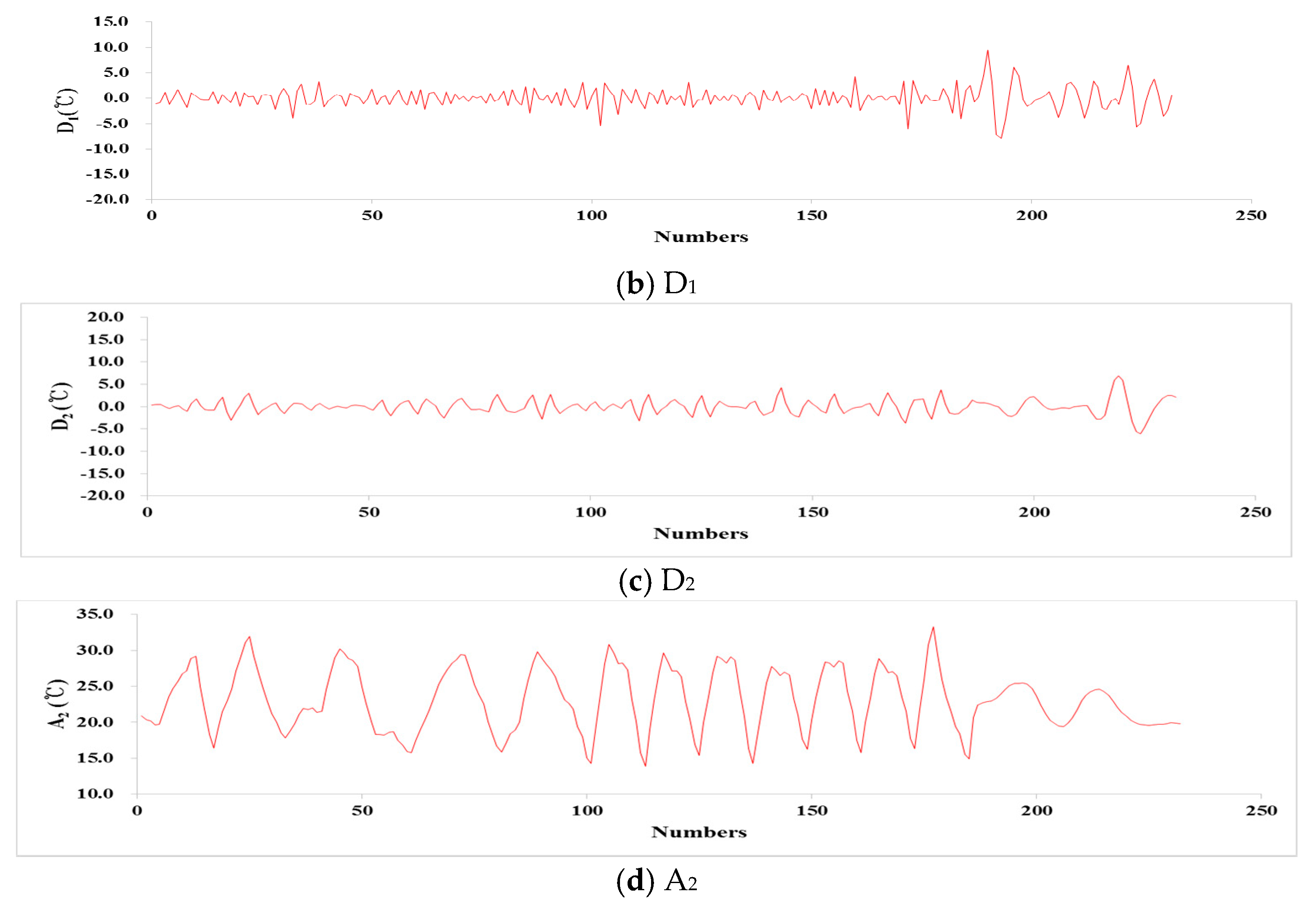
2.3. Discrete Wavelet Transform (DWT)
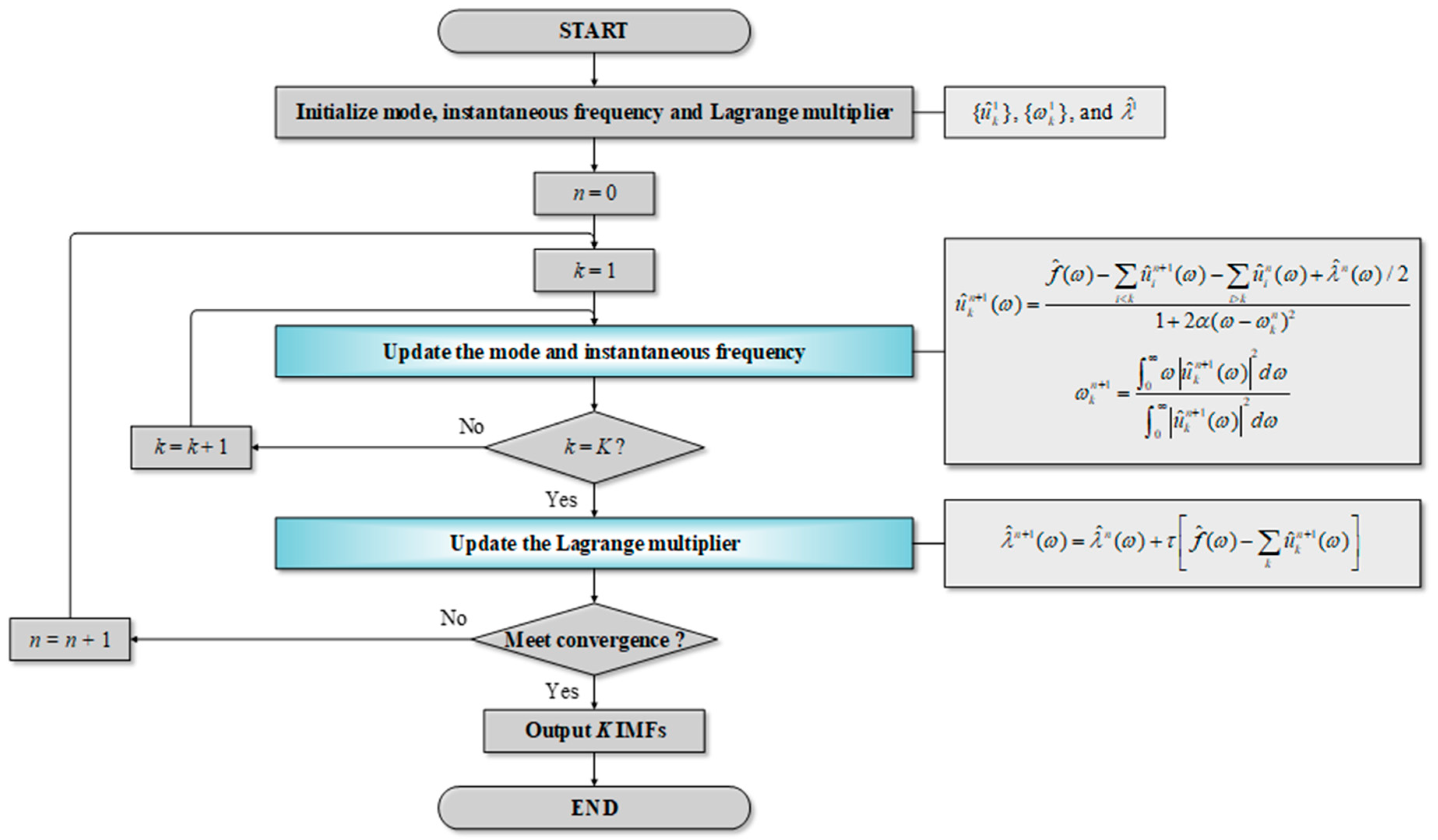
2.4. Variational Mode Decomposition (VMD)
2.5. Hybrid Modeling Using DWT and VMD Approaches
2.6. Performance Evaluation of Models
- Root mean square error (RMSE):
- Nash–Sutcliffe coefficient (NSE):
- Willmott’s index of agreement (WI):
- Mean absolute error (MAE):
- Coefficient of determination (R2):where and are the observed and predicted values, respectively; and are the average of observed and predicted values, respectively; and n is the length of time series data. The discrepancy between observed and predicted values can be shown using the RMSE criterion. A value of zero reflects perfect prediction. The RMSE criterion must be used for model evaluation to obtain accuracy in absolute units [80]. NSE is taken into account to evaluate the ability of predicting models [81]. If the squared difference between observed and predicted DO values is relatively large to concur with the variance in the observed DO values, then the NSE criterion will be zero. If the NSE criterion is negative, the results indicate that the observed mean is a better predictor than the model [81,82]. If the NSE criterion is equal to one, it indicates a perfect model [83]. The WI criterion varies between zero and one. WI calculates the ratio of mean square error (MSE) and can provide an advantage over the RMSE [84,85,86]. The MAE criterion can provide better information for a model’s prediction. The MAE cannot be weighted towards higher or lower magnitudes. However, it evaluates all derivations from observed DO values in an equal manner [87].
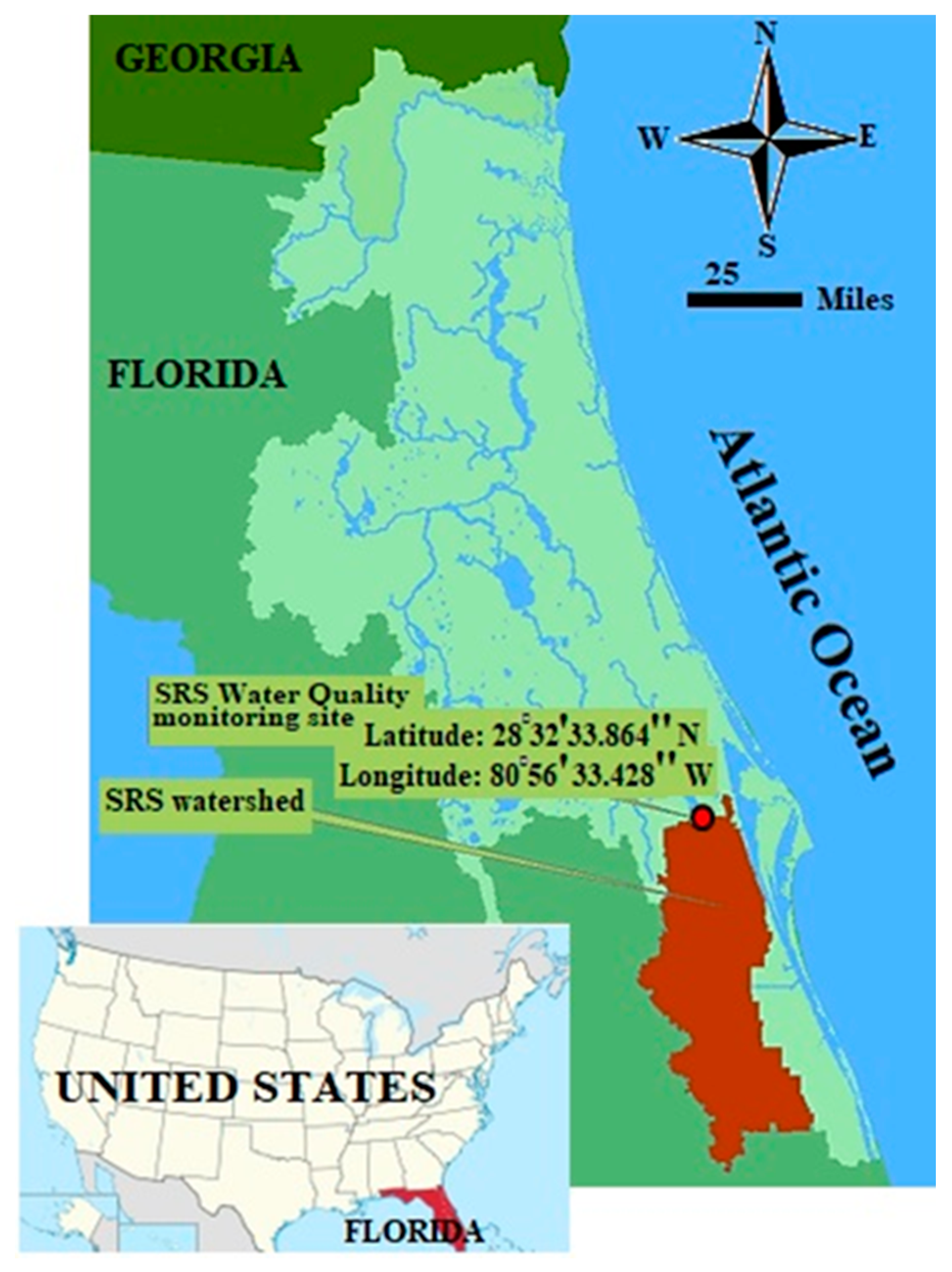
3. Case Study
4. Application and Results
4.1. Setting up the Standalone Models
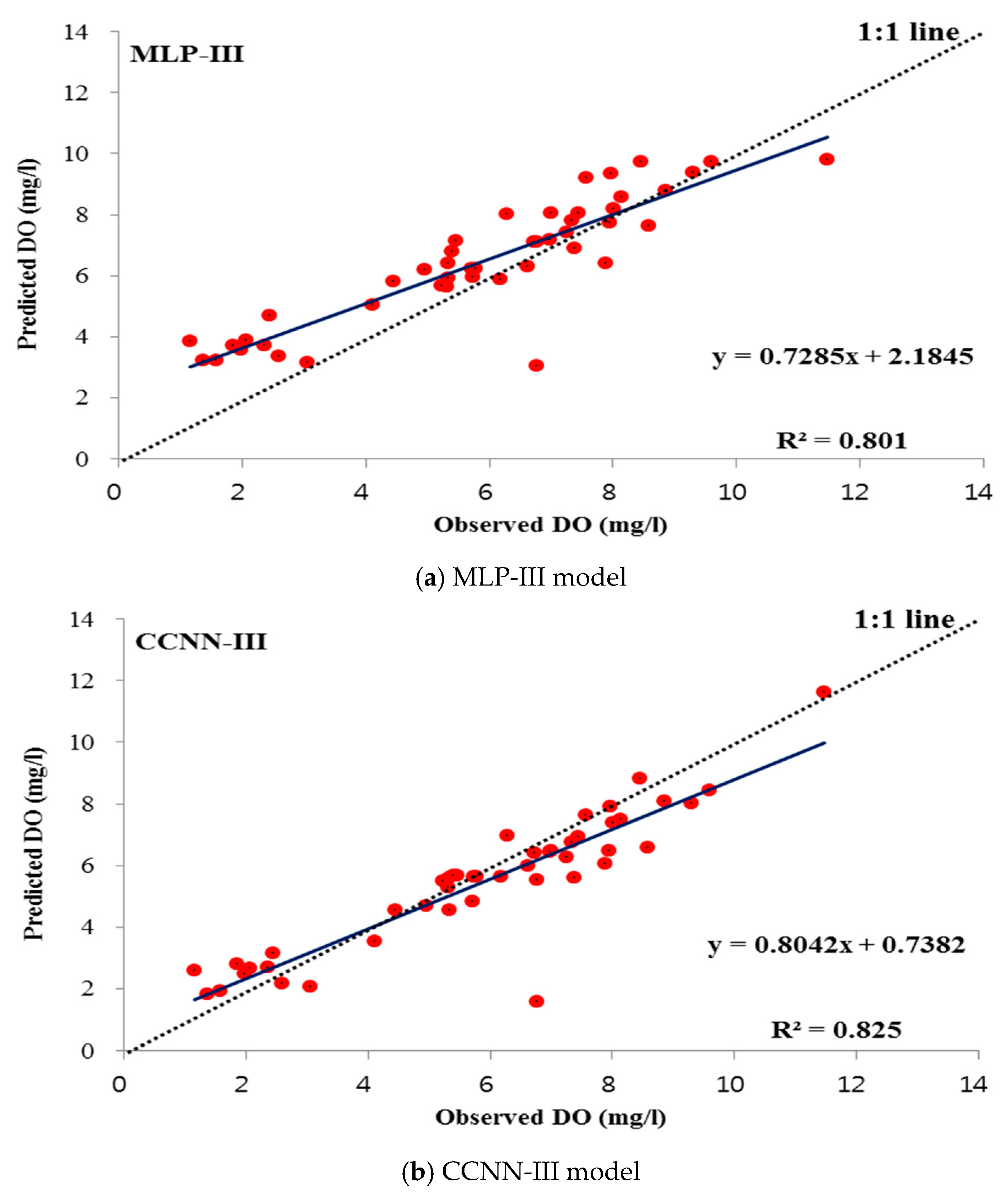
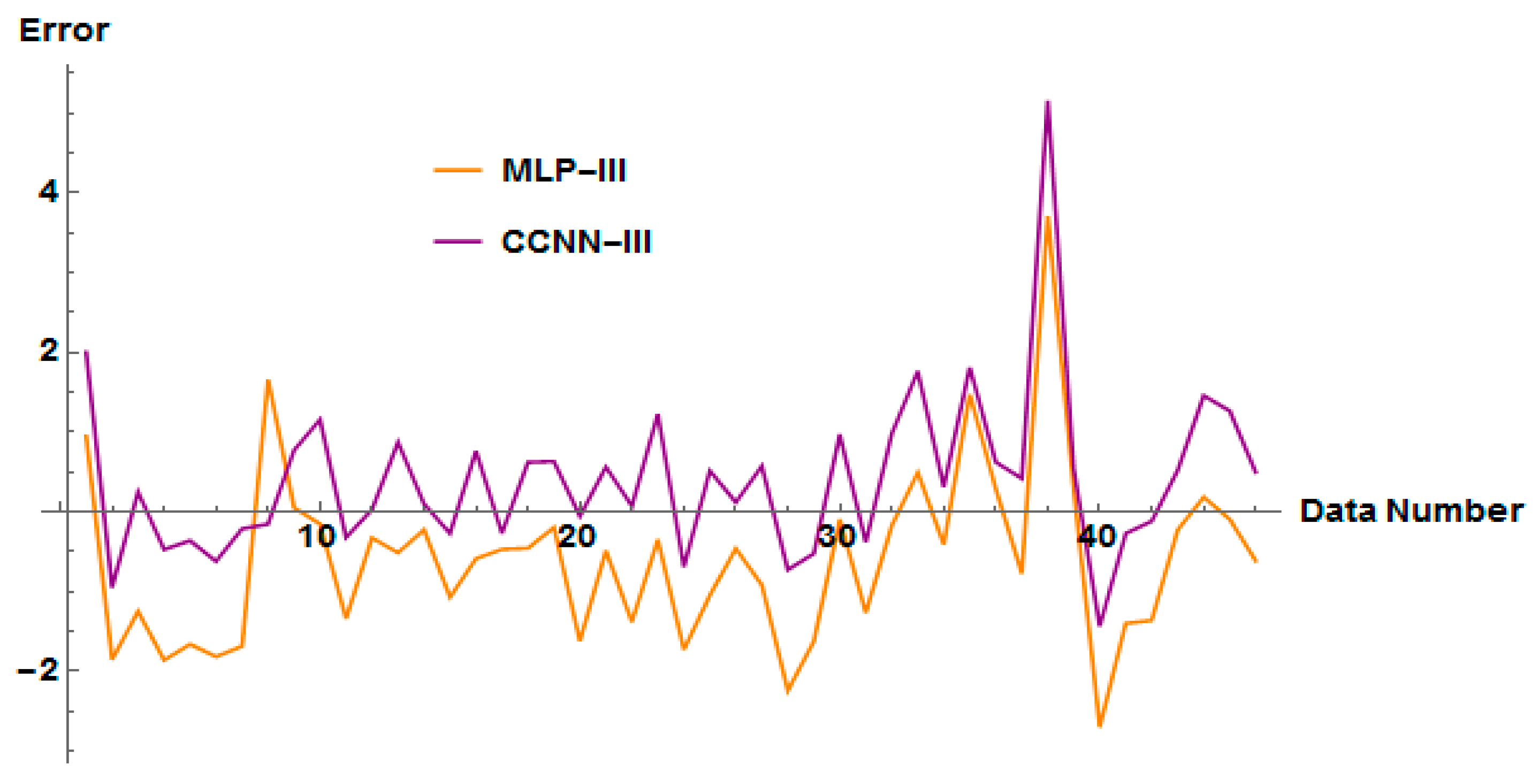
4.2. Performance of Standalone Models
4.3. Performance of Hybrid Models
4.3.1. DWT-Based Soft Computing Models
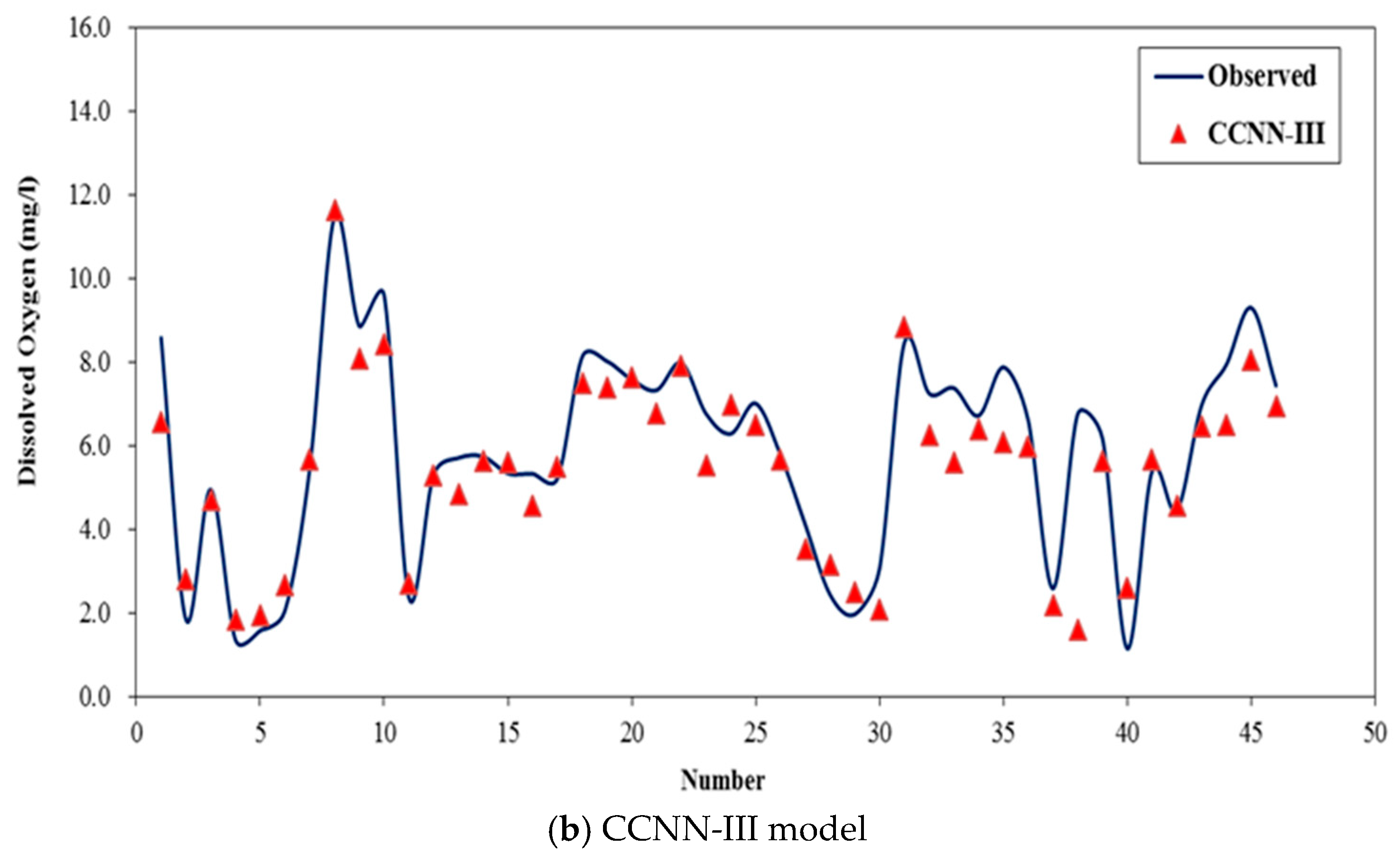
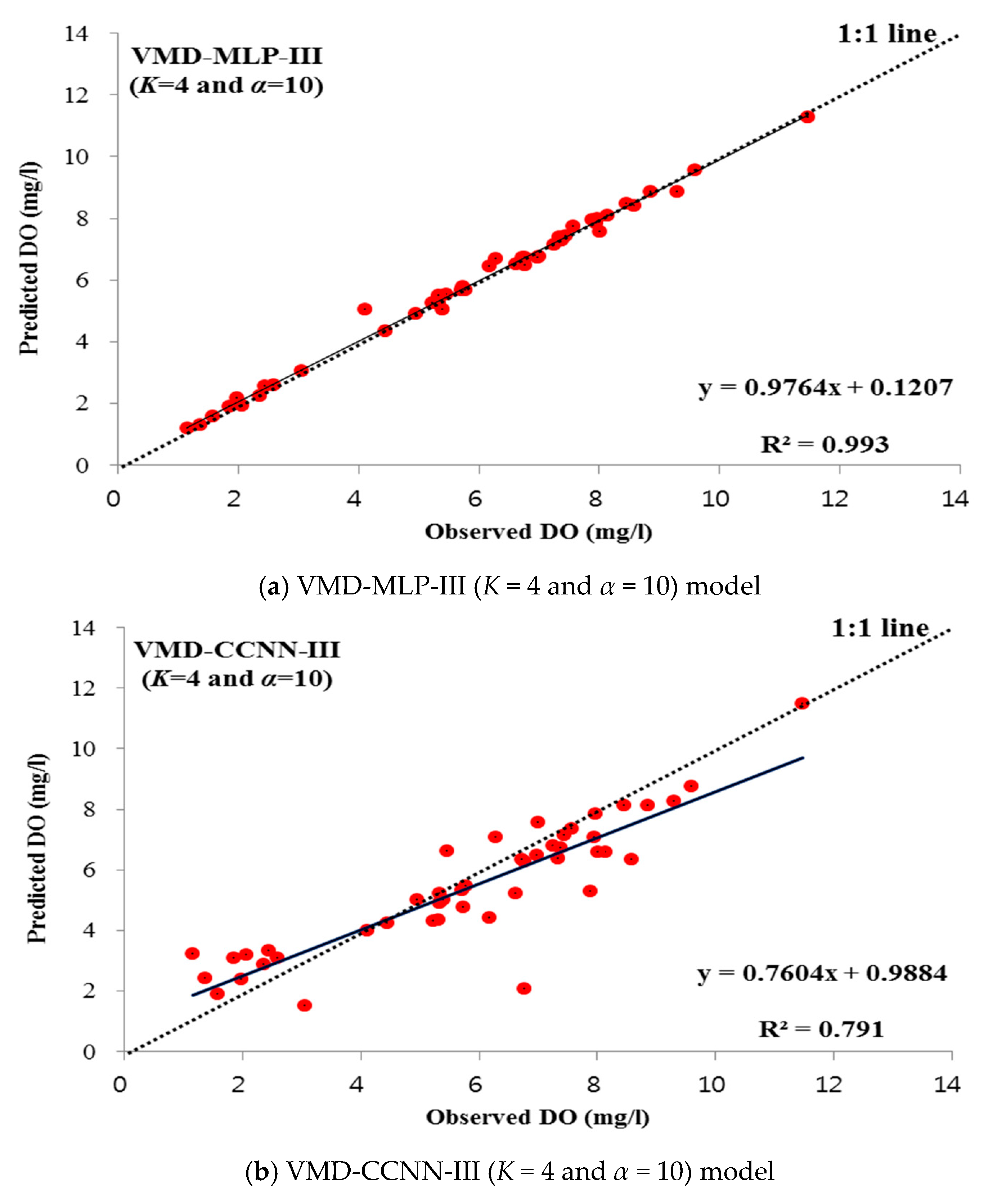
4.3.2. VMD-Based Soft Computing Models
4.4. Diagnostic Analysis
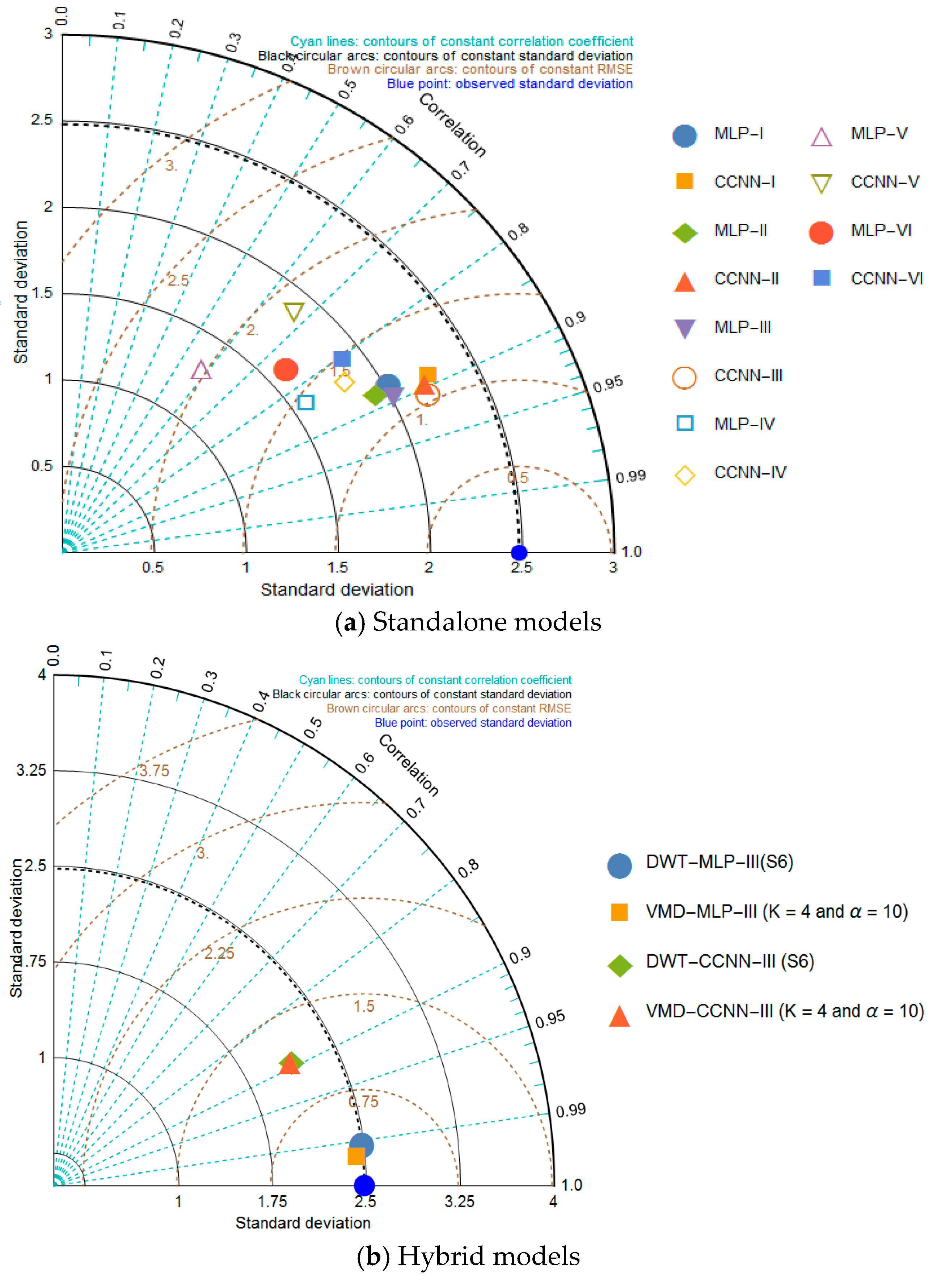
4.4.1. Taylor Diagram
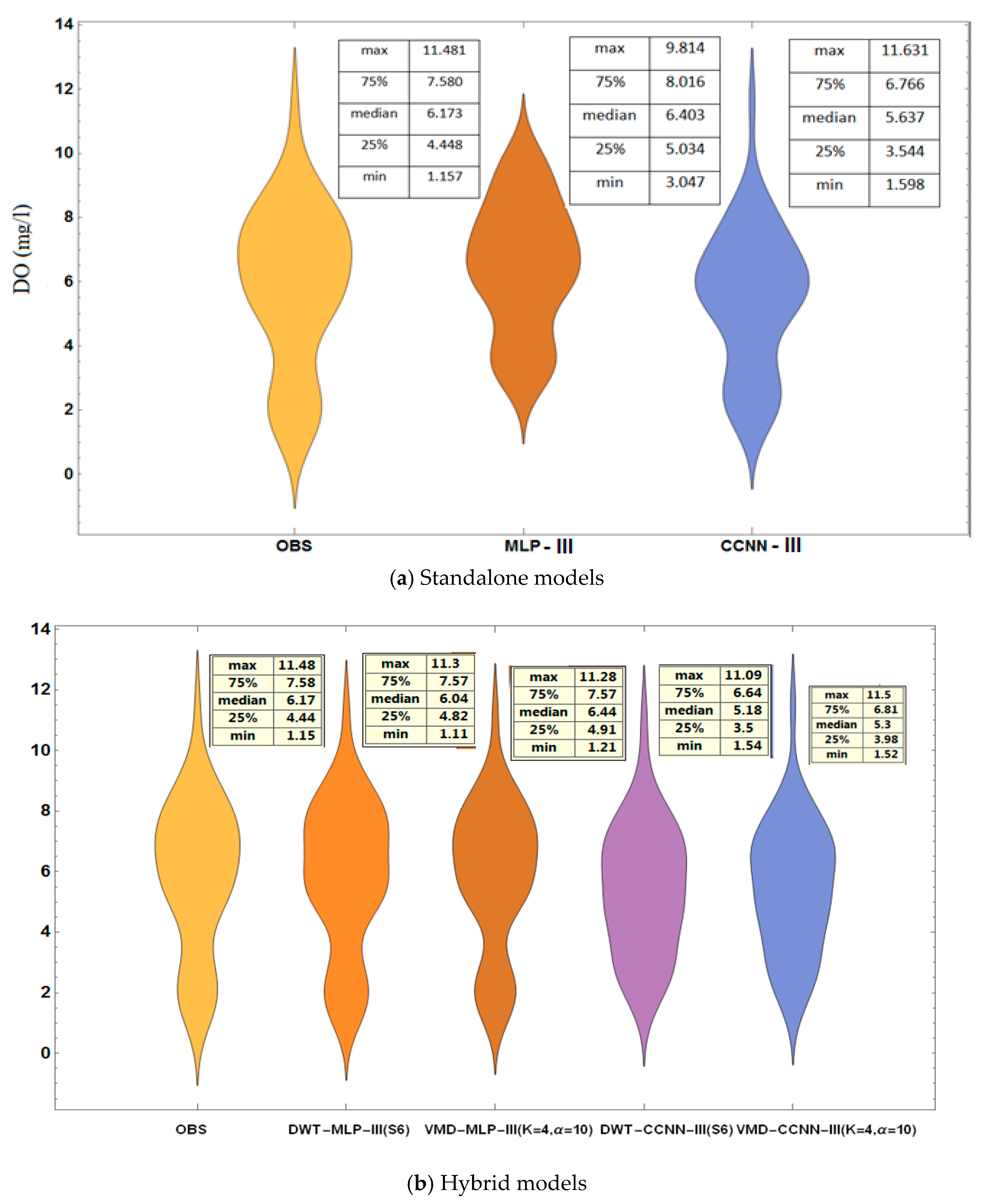
4.4.2. Violin Plot
5. Conclusions
Author Contributions
Funding
Acknowledgments
Conflicts of Interest
References
- Liou, S.M.; Lo, S.L.; Wang, S.H. A generalized water quality index for Taiwan. Environ. Monit. Assess. 2004, 96, 32–35. [Google Scholar] [CrossRef]
- Khalil, B.; Ouarda, T.B.M.J.; St-Hilaire, A. Estimation of water quality characteristics at ungauged sites using artificial neural networks and canonical correlation analysis. J. Hydrol. 2011, 405, 277–287. [Google Scholar] [CrossRef]
- Najah, A.; Elshafie, A.; Karim, O.A.; Jaffar, O. Prediction of Johor River water quality parameters using artificial neural networks. Eur. J. Sci. Res. 2009, 28, 422–435. [Google Scholar]
- Singh, K.P.; Basant, A.; Malik, A.; Jain, G. Artificial neural network modeling of the river water quality—A case study. Ecol. Model. 2009, 220, 888–895. [Google Scholar] [CrossRef]
- Ranković, V.; Radulović, J.; Radojević, I.; Ostojić, A.; Čomić, L. Neural network modeling of dissolved oxygen in the Gruža reservoir, Serbia. Ecol. Model. 2010, 221, 1239–1244. [Google Scholar] [CrossRef]
- Xia, M.; Craig, P.M.; Schaeffer, B.; Stoddard, A.; Liu, Z.; Peng, M.; Zhang, H.; Wallen, C.M.; Bailey, N.; Mandrup-Poulsen, J. Influence of physical forcing on bottom-water dissolved oxygen within Caloosahatchee River Estuary, Florida. J. Environ. Eng. 2010, 136, 1032–1044. [Google Scholar] [CrossRef]
- Xia, M.; Jiang, L. Influence of wind and river discharge on the hypoxia in a shallow bay. Ocean Dyn. 2015, 65, 665–678. [Google Scholar] [CrossRef]
- Olyaie, E.; Abyaneh, H.Z.; Mehr, A.D. A comparative analysis among computational intelligence techniques for dissolved oxygen prediction in Delaware River. Geosci. Front. 2017, 8, 517–527. [Google Scholar] [CrossRef] [Green Version]
- Gazzaz, N.M.; Yusoff, M.K.; Aris, A.Z.; Juahir, H.; Ramli, M.F. Artificial neural network modeling of the water quality index for Kinta River (Malaysia) using water quality variables as predictors. Mar. Pollut. Bull. 2012, 64, 2409–2420. [Google Scholar] [CrossRef]
- Ay, M.; Kisi, O. Modeling of dissolved oxygen concentration using different neural network techniques in Foundation Creek, El Paso County, Colorado. J. Environ. Eng. 2011, 138, 654–662. [Google Scholar] [CrossRef]
- Zou, R.; Lung, W.S.; Wu, J. An adaptive neural network embedded genetic algorithm approach for inverse water quality modeling. Water Resour. Res. 2007, 43, W08427. [Google Scholar] [CrossRef]
- Xu, L.; Liu, S. Study of short-term water quality prediction model based on wavelet neural network. Math. Comput. Model. 2013, 58, 807–813. [Google Scholar] [CrossRef]
- Sen, M.K.; Stoffa, P.L. Global Optimization Methods in Geophysical Inversion; Cambridge University Press: Cambridge, UK, 2013. [Google Scholar]
- Maier, H.R.; Dandy, G.C. The use of artificial neural networks for the prediction of water quality parameters. Water Resour. Res. 1996, 32, 1013–1022. [Google Scholar] [CrossRef]
- Zhang, Q.; Stanley, S.J. Forecasting raw-water quality parameters for the North Saskatchewan River by neural network modeling. Water Res. 1997, 31, 2340–2350. [Google Scholar] [CrossRef]
- Aguilera, P.A.; Frenich, A.G.; Torres, J.A.; Castro, H.; Vidal, J.M.; Canton, M. Application of the Kohonen neural network in coastal water management: Methodological development for the assessment and prediction of water quality. Water Res. 2001, 35, 4053–4062. [Google Scholar] [CrossRef]
- Zhang, Y.; Pulliainen, J.; Koponen, S.; Hallikainen, M. Application of an empirical neural network to surface water quality estimation in the Gulf of Finland using combined optical data and microwave data. Remote Sens. Environ. 2002, 81, 327–336. [Google Scholar] [CrossRef]
- Zou, R.; Lung, W.S.; Guo, H. Neural network embedded Monte Carlo approach for water quality modeling under input information uncertainty. J. Comput. Civ. Eng. 2002, 16, 135–142. [Google Scholar] [CrossRef]
- Ha, H.; Stenstrom, M.K. Identification of land use with water quality data in stormwater using a neural network. Water Res. 2003, 37, 4222–4230. [Google Scholar] [CrossRef]
- Diamantopoulou, M.J.; Papamichail, D.M.; Antonopoulos, V.Z. The use of a neural network technique for the prediction of water quality parameters. Oper. Res. 2005, 5, 115–125. [Google Scholar] [CrossRef]
- Diamantopoulou, M.J.; Antonopoulos, V.Z.; Papamichail, D.M. Cascade correlation artificial neural networks for estimating missing monthly values of water quality parameters in rivers. Water Resour. Manag. 2007, 21, 649–662. [Google Scholar] [CrossRef]
- Kuo, J.T.; Hsieh, M.H.; Lung, W.S.; She, N. Using artificial neural network for reservoir eutrophication prediction. Ecol. Model. 2007, 200, 171–177. [Google Scholar] [CrossRef]
- Zhao, Y.; Nan, J.; Cui, F.Y.; Guo, L. Water quality forecast through application of BP neural network at Yuqiao reservoir. J. Zhejiang Univ.-Sci. A 2007, 8, 1482–1487. [Google Scholar] [CrossRef]
- Dogan, E.; Sengorur, B.; Koklu, R. Modeling biological oxygen demand of the Melen River in Turkey using an artificial neural network technique. J. Environ. Manag. 2009, 90, 1229–1235. [Google Scholar] [CrossRef] [PubMed]
- Singh, K.P.; Basant, N.; Gupta, S. Support vector machines in water quality management. Anal. Chim. Acta 2011, 703, 152–162. [Google Scholar] [CrossRef] [PubMed]
- Han, H.G.; Chen, Q.L.; Qiao, J.F. An efficient self-organizing RBF neural network for water quality prediction. Neural Netw. 2011, 24, 717–725. [Google Scholar] [CrossRef] [PubMed]
- Ay, M.; Kisi, O. Modelling of chemical oxygen demand by using ANNs, ANFIS and k-means clustering techniques. J. Hydrol. 2014, 511, 279–289. [Google Scholar] [CrossRef]
- Li, J.; Abdulmohsin, H.A.; Hasan, S.S.; Kaiming, L.; Al-Khateeb, B.; Ghareb, M.I.; Mohammed, M.N. Hybrid soft computing approach for determining water quality indicator: Euphrates River. Neural Comput. Appl. 2019, 31, 827–837. [Google Scholar] [CrossRef]
- Sengorur, B.; Dogan, E.; Koklu, R.; Samandar, A. Dissolved oxygen estimation using artificial neural network for water quality control. Fresenius Environ. Bull. 2006, 15, 1064–1067. [Google Scholar]
- Wen, X.; Fang, J.; Diao, M.; Zhang, C. Artificial neural network modeling of dissolved oxygen in the Heihe River, Northwestern China. Environ. Monit. Assess. 2013, 185, 4361–4371. [Google Scholar] [CrossRef]
- Raheli, B.; Aalami, M.T.; El-Shafie, A.; Ghorbani, M.A.; Deo, R.C. Uncertainty assessment of the multilayer perceptron (MLP) neural network model with implementation of the novel hybrid MLP-FFA method for prediction of biochemical oxygen demand and dissolved oxygen: A case study of Langat River. Environ. Earth Sci. 2017, 76, 503. [Google Scholar] [CrossRef]
- Chen, D.; Lu, J.; Shen, Y. Artificial neural network modelling of concentrations of nitrogen, phosphorus and dissolved oxygen in a non-point source polluted river in Zhejiang Province, southeast China. Hydrol. Process. 2010, 24, 290–299. [Google Scholar] [CrossRef]
- Soyupak, S.; Karaer, F.; Gürbüz, H.; Kivrak, E.; Sentürk, E.; Yazici, A. A neural network-based approach for calculating dissolved oxygen profiles in reservoirs. Neural Comput. Appl. 2003, 12, 166–172. [Google Scholar] [CrossRef]
- Schmid, B.H.; Koskiaho, J. Artificial neural network modeling of dissolved oxygen in a wetland pond: The case of Hovi, Finland. J. Hydrol. Eng. 2006, 11, 188–192. [Google Scholar] [CrossRef]
- Ranković, V.; Radulović, J.; Radojević, I.; Ostojić, A.; Čomić, L. Prediction of dissolved oxygen in reservoirs using adaptive network-based fuzzy inference system. J. Hydroinform. 2012, 14, 167–179. [Google Scholar] [CrossRef]
- Akkoyunlu, A.; Altun, H.; Cigizoglu, H.K. Depth-integrated estimation of dissolved oxygen in a lake. J. Environ. Eng. 2011, 137, 961–967. [Google Scholar] [CrossRef]
- Chen, W.B.; Liu, W.C. Artificial neural network modeling of dissolved oxygen in reservoir. Environ. Monit. Assess. 2014, 186, 1203–1217. [Google Scholar] [CrossRef] [PubMed]
- Faruk, D.Ö. A hybrid neural network and ARIMA model for water quality time series prediction. Eng. Appl. Artif. Intell. 2010, 23, 586–594. [Google Scholar] [CrossRef]
- Han, H.G.; Qiao, J.F.; Chen, Q.L. Model predictive control of dissolved oxygen concentration based on a self-organizing RBF neural network. Control Eng. Pract. 2012, 20, 465–476. [Google Scholar] [CrossRef]
- Martí, P.; Shiri, J.; Duran-Ros, M.; Arbat, G.; De Cartagena, F.R.; Puig-Bargués, J. Artificial neural networks vs. gene expression programming for estimating outlet dissolved oxygen in micro-irrigation sand filters fed with effluents. Comput. Electron. Agric. 2013, 99, 176–185. [Google Scholar] [CrossRef]
- Antanasijević, D.; Pocajt, V.; Perić-Grujić, A.; Ristić, M. Modelling of dissolved oxygen in the Danube River using artificial neural networks and Monte Carlo Simulation uncertainty analysis. J. Hydrol. 2014, 519, 1895–1907. [Google Scholar] [CrossRef]
- Heddam, S. Modeling hourly dissolved oxygen concentration (DO) using two different adaptive neuro-fuzzy inference systems (ANFIS): A comparative study. Environ. Monit. Assess. 2014, 186, 597–619. [Google Scholar] [CrossRef] [PubMed]
- Najah, A.; El-Shafie, A.; Karim, O.A.; El-Shafie, A.H. Performance of ANFIS versus MLP-NN dissolved oxygen prediction models in water quality monitoring. Environ. Sci. Pollut. Res. 2014, 21, 1658–1670. [Google Scholar] [CrossRef] [PubMed]
- Nemati, S.; Fazelifard, M.H.; Terzi, Ö.; Ghorbani, M.A. Estimation of dissolved oxygen using data-driven techniques in the Tai Po River, Hong Kong. Environ. Earth Sci. 2015, 74, 4065–4073. [Google Scholar] [CrossRef]
- Keshtegar, B.; Heddam, S. Modeling daily dissolved oxygen concentration using modified response surface method and artificial neural network: A comparative study. Neural Comput. Appl. 2018, 30, 2995–3006. [Google Scholar] [CrossRef]
- Tomić, A.S.; Antanasijević, D.; Ristić, M.; Perić-Grujić, A.; Pocajt, V. A linear and non-linear polynomial neural network modeling of dissolved oxygen content in surface water: Inter- and extrapolation performance with inputs’ significance analysis. Sci. Total Environ. 2018, 610, 1038–1046. [Google Scholar] [CrossRef] [PubMed]
- Liu, S.; Xu, L.; Li, D.; Li, Q.; Jiang, Y.; Tai, H.; Zeng, L. Prediction of dissolved oxygen content in river crab culture based on least squares support vector regression optimized by improved particle swarm optimization. Comput. Electron. Agric. 2013, 95, 82–91. [Google Scholar] [CrossRef]
- Liu, S.; Xu, L.; Jiang, Y.; Li, D.; Chen, Y.; Li, Z. A hybrid WA–CPSO-LSSVR model for dissolved oxygen content prediction in crab culture. Eng. Appl. Artif. Intell. 2014, 29, 114–124. [Google Scholar] [CrossRef]
- Alizadeh, M.J.; Kavianpour, M.R. Development of wavelet-ANN models to predict water quality parameters in Hilo Bay, Pacific Ocean. Mar. Pollut. Bull. 2015, 98, 171–178. [Google Scholar] [CrossRef]
- Ravansalar, M.; Rajaee, T.; Ergil, M. Prediction of dissolved oxygen in River Calder by noise elimination time series using wavelet transform. J. Exp. Theor. Artif. Intell. 2016, 28, 689–706. [Google Scholar] [CrossRef]
- Fijani, E.; Barzegar, R.; Deo, R.; Tziritis, E.; Konstantinos, S. Design and implementation of a hybrid model based on two-layer decomposition method coupled with extreme learning machines to support real-time environmental monitoring of water quality parameters. Sci. Total Environ. 2019, 648, 839–853. [Google Scholar] [CrossRef]
- Huang, Y.; Schmitt, F.G. Time dependent intrinsic correlation analysis of temperature and dissolved oxygen time series using empirical mode decomposition. J. Mar. Syst. 2014, 130, 90–100. [Google Scholar] [CrossRef]
- McClelland, J.L.; Rumelhart, D.E. Explorations in Parallel Distributed Processing: A Handbook of Models, Programs, and Exercises; MIT Press: Cambridge, MA, USA, 1989. [Google Scholar]
- Haykin, S. Neural Networks and Learning Machines, 3rd ed.; Prentice Hall: Upper Saddle River, NJ, USA, 2009. [Google Scholar]
- Kim, S.; Shiri, J.; Kisi, O. Pan evaporation modeling using neural computing approach for different climatic zones. Water Resour. Manag. 2012, 26, 3231–3249. [Google Scholar] [CrossRef]
- Kim, S.; Shiri, J.; Kisi, O.; Singh, V.P. Estimating daily pan evaporation using different data-driven methods and lag-time patterns. Water Resour. Manag. 2013, 27, 2267–2286. [Google Scholar] [CrossRef]
- Kim, S.; Singh, V.P. Spatial disaggregation of areal rainfall using two different artificial neural networks. Water 2015, 7, 2707–2727. [Google Scholar] [CrossRef]
- Deo, R.C.; Sahin, M. An extreme learning machine model for the simulation of monthly mean streamflow water level in eastern Queensland. Environ. Monit. Assess. 2016, 188, 90. [Google Scholar] [CrossRef] [PubMed]
- Deo, R.C.; Sahin, M. Forecasting long-term global solar radiation with an ANN algorithm coupled with satellite-derived (MODIS) land surface temperature (LST) for regional locations in Queensland. Renew. Sustain. Energy Rev. 2017, 72, 828–848. [Google Scholar] [CrossRef]
- Fahimi, K.; Seyedhosseini, S.M.; Makui, A. Simultaneous competitive supply chain network design with continuous attractiveness variables. Comput. Ind. Eng. 2017, 107, 235–250. [Google Scholar] [CrossRef]
- Zounemat-Kermani, M. Assessment of several nonlinear methods in forecasting suspended sediment concentration in streams. Hydrol. Res. 2017, 48, 1240–1252. [Google Scholar] [CrossRef]
- Nourani, V.; Baghanam, A.H.; Adamowski, J.; Gebremichael, M. Using self-organizing maps and wavelet transforms for space–time pre-processing of satellite precipitation and runoff data in neural network based rainfall–runoff modeling. J. Hydrol. 2013, 476, 228–243. [Google Scholar] [CrossRef]
- Barzegar, R.; Moghaddam, A.A.; Baghban, H. A supervised committee machine artificial intelligent for improving DRASTIC method to assess groundwater contamination risk: A case study from Tabriz plain aquifer, Iran. Stoch. Environ. Res. Risk Assess. 2016, 30, 883–899. [Google Scholar] [CrossRef]
- Fahlman, S.E.; Lebiere, C. The cascade-correlation learning architecture. In Advances in Neural Information Processing Systems 2; Morgan Kaufmann Publishers Inc.: San Francisco, CA, USA, 1990; pp. 524–532. [Google Scholar]
- Kim, S.; Singh, V.P.; Seo, Y. Evaluation of pan evaporation modeling with two different neural networks and weather station data. Theor. Appl. Climatol. 2014, 117, 1–13. [Google Scholar] [CrossRef]
- Karunanithi, N.; Grenney, W.J.; Whitley, D.; Bovee, K. Neural networks for river flow prediction. J. Comput. Civ. Eng. 1994, 8, 201–220. [Google Scholar] [CrossRef]
- Thirumalaiah, K.; Deo, M.C. River stage forecasting using artificial neural networks. J. Hydrol. Eng. 1998, 3, 26–32. [Google Scholar] [CrossRef]
- Mallat, S.G. A theory for multiresolution signal decomposition: The wavelet representation. IEEE Trans. Pattern Anal. Mach. Intell. 1989, 11, 674–693. [Google Scholar] [CrossRef]
- Kisi, O.; Cimen, M. A wavelet-support vector machine conjunction model for monthly streamflow forecasting. J. Hydrol. 2011, 399, 132–140. [Google Scholar] [CrossRef]
- Nourani, V.; Alami, M.T.; Aminfar, M.H. A combined neural-wavelet model for prediction of Ligvanchai watershed precipitation. Eng. Appl. Artif. Intell. 2009, 22, 466–472. [Google Scholar] [CrossRef]
- Kim, S.; Singh, V.P.; Lee, C.J.; Seo, Y. Modeling the physical dynamics of daily dew point temperature using soft computing techniques. KSCE J. Civ. Eng. 2015, 19, 1930–1940. [Google Scholar] [CrossRef]
- Seo, Y.; Kim, S.; Kisi, O.; Singh, V.J. Daily water level forecasting using wavelet decomposition and artificial intelligence techniques. J. Hydrol. 2015, 520, 224–243. [Google Scholar] [CrossRef]
- Seo, Y.; Kim, S.; Singh, V. Machine learning models coupled with variational mode decomposition: A new approach for modeling daily rainfall-runoff. Atmosphere 2018, 9, 251. [Google Scholar] [CrossRef]
- González-Audícana, M.; Otazu, X.; Fors, O.; Seco, A. Comparison between Mallat’s and the ‘à trous’ discrete wavelet transform based algorithms for the fusion of multispectral and panchromatic images. Int. J. Remote Sens. 2005, 26, 595–614. [Google Scholar] [CrossRef]
- Kim, S.; Seo, Y.; Rezaie-Balf, M.; Kisi, O.; Ghorbani, M.A.; Singh, V.P. Evaluation of daily solar radiation flux using soft computing approaches based on different meteorological information: Peninsula vs. continent. Theor. Appl. Climatol. 2018, 1–20. [Google Scholar] [CrossRef]
- Nason, G. Wavelet Methods in Statistics with R; Springer: New York, NY, USA, 2010. [Google Scholar]
- Percival, D.B.; Walden, A.T. Wavelet Methods for Time Series Analysis; Cambridge University Press: New York, NY, USA, 2006; Volume 4. [Google Scholar]
- Dragomiretskiy, K.; Zosso, D. Variational mode decomposition. IEEE Trans. Signal Process. 2014, 62, 531–544. [Google Scholar] [CrossRef]
- Luenberger, D.G.; Ye, Y. Linear and Nonlinear Programming, 3rd ed.; Springer: New York, NY, USA, 2008. [Google Scholar]
- Deo, R.C.; Şahin, M.; Adamowski, J.F.; Mi, J. Universally deployable extreme learning machines integrated with remotely sensed MODIS satellite predictors over Australia to forecast global solar radiation: A new approach. Renew. Sustain. Energy Rev. 2019, 104, 235–261. [Google Scholar] [CrossRef]
- Nash, J.E.; Sutcliffe, J.V. River flow forecasting through conceptual models part I—A discussion of principles. J. Hydrol. 1970, 10, 282–290. [Google Scholar] [CrossRef]
- Wilcox, B.P.; Rawls, W.J.; Brakensiek, D.L.; Wight, J.R. Predicting runoff from rangeland catchments: A comparison of two models. Water Resour. Res. 1990, 26, 2401–2410. [Google Scholar] [CrossRef]
- Legates, D.R.; McCabe, G.J. Evaluating the use of “goodness-of-fit” measures in hydrologic and hydroclimatic model validation. Water Resour. Res. 1999, 35, 233–241. [Google Scholar] [CrossRef]
- Willmott, C.J. On the evaluation of model performance in physical geography. In Spatial Statistics and Models; Springer: Dordrecht, The Netherlands, 1984; pp. 443–460. [Google Scholar]
- Willmott, C.J.; Matsuura, K. Advantages of the mean absolute error (MAE) over the root mean square error (RMSE) in assessing average model performance. Clim. Res. 2005, 30, 79–82. [Google Scholar] [CrossRef]
- Willmott, C.J.; Robeson, S.M.; Matsuura, K. A refined index of model performance. Int. J. Climatol. 2012, 32, 2088–2094. [Google Scholar] [CrossRef]
- Chai, T.; Draxler, R.R. Root mean square error (RMSE) or mean absolute error (MAE)?—Arguments against avoiding RMSE in the literature. Geosci. Model Dev. 2014, 7, 1247–1250. [Google Scholar] [CrossRef]
- Tsoukalas, L.H.; Uhrig, R.E. Fuzzy and Neural Approaches in Engineering; John Wiley & Sons: New York, NY, USA, 1997. [Google Scholar]
- Adamowski, J.; Sun, K. Development of a coupled wavelet transform and neural network method for flow forecasting of non-perennial rivers in semi-arid watersheds. J. Hydrol. 2010, 390, 85–91. [Google Scholar] [CrossRef]
- Tiwari, M.K.; Chatterjee, C. Development of an accurate and reliable hourly flood forecasting model using wavelet-bootstrap-ANN (WBANN) hybrid approach. J. Hydrol. 2010, 394, 458–470. [Google Scholar] [CrossRef]
- Taylor, K.E. Summarizing multiple aspects of model performance in a single diagram. J. Geophys. Res. Atmos. 2001, 106, 7183–7192. [Google Scholar] [CrossRef]
- IPCC. Climate change 2007: The physical science basis. Agenda 2007, 6, 333. [Google Scholar]
- Gleckler, P.J.; Taylor, K.E.; Doutriaux, C. Performance metrics for climate models. J. Geophys. Res. Atmos. 2008, 113. [Google Scholar] [CrossRef]
- Heo, K.Y.; Ha, K.J.; Yun, K.S.; Lee, S.S.; Kim, H.J.; Wang, B. Methods for uncertainty assessment of climate models and model predictions over East Asia. Int. J. Climatol. 2014, 34, 377–390. [Google Scholar] [CrossRef]
- Sigaroodi, S.K.; Chen, Q.; Ebrahimi, S.; Nazari, A.; Choobin, B. Long-term precipitation forecast for drought relief using atmospheric circulation factors: A study on the Maharloo Basin in Iran. Hydrol. Earth Syst. Sci. 2014, 18, 1995–2006. [Google Scholar] [CrossRef]


| Variable | Unit | Min | Max | Median | Mean | SD | CV | CC | |
|---|---|---|---|---|---|---|---|---|---|
| Input | Cl | mg/L | 40.000 | 850.000 | 200.000 | 247.649 | 164.973 | 0.666 | 0.418 |
| NOx | mg/L | 0.001 | 0.460 | 0.072 | 0.089 | 0.087 | 0.978 | 0.554 | |
| TDS | 134.000 | 1950.000 | 559.500 | 642.362 | 355.163 | 0.553 | 0.394 | ||
| pH | Standard Units | 6.100 | 8.220 | 7.180 | 7.148 | 0.421 | 0.059 | 0.760 | |
| WT | °C | 8.980 | 32.220 | 23.510 | 232.378 | 5.211 | 0.022 | −0.544 | |
| Output | DO | mg/L | 0.090 | 11.480 | 5.920 | 5.485 | 2.565 | 0.468 | 1.000 |
| ID of the Input Combination | Input | Input No. | Output |
|---|---|---|---|
| I | Cl, NOx, TDS, pH, WT | 5 | DO |
| II | Cl, NOx, pH, WT | 4 | DO |
| III | NOx, pH, WT | 3 | DO |
| IV | WT, NOx | 2 | DO |
| V | WT | 1 | DO |
| VI | PH | 1 | DO |
| Model | ID | Topology | Training Phase | Testing Phase | ||||||||
|---|---|---|---|---|---|---|---|---|---|---|---|---|
| RMSE (mg/L) | NSE | WI | R2 | MAE (mg/L) | RMSE (mg/L) | NSE | WI | R2 | MAE (mg/L) | |||
| MLP | I | 5-2-1 | 1.211 * | 0.778 * | 0.933 * | 0.781 * | 0.924 * | 1.425 | 0.663 | 0.897 | 0.769 | 1.126 |
| II | 4-2-1 | 1.237 | 0.768 | 0.930 | 0.769 | 0.938 | 1.359 | 0.694 | 0.902 | 0.774 | 1.062 | |
| III ** | 3-4-1 | 1.306 | 0.742 | 0.918 | 0.752 | 0.994 | 1.261 * | 0.736* | 0.919 * | 0.801 * | 0.989 * | |
| IV | 2-4-1 | 1.830 | 0.493 | 0.817 | 0.496 | 1.437 | 1.427 | 0.662 | 0.868 | 0.707 | 1.072 | |
| V | 1-1-1 | 2.138 | 0.308 | 0.676 | 0.310 | 1.810 | 2.007 | 0.332 | 0.684 | 0.335 | 1.633 | |
| VI | 1-1-1 | 1.585 | 0.620 | 0.871 | 0.620 | 1.264 | 2.138 | 0.242 | 0.741 | 0.568 | 1.773 | |
| CCNN | I | 5-1-1 | 1.227 | 0.772 | 0.933 | 0.773 | 0.953 | 1.172 | 0.772 | 0.935 | 0.795 | 0.790 |
| II | 4-1-1 | 1.196 * | 0.783 * | 0.937 * | 0.785 * | 0.881 * | 0.581 | 0.773 | 0.935 | 0.801 | 0.195 | |
| III ** | 3-2-1 | 1.245 | 0.765 | 0.931 | 0.767 | 0.922 | 0.550 * | 0.797 * | 0.942 * | 0.825 * | 0.185 * | |
| IV | 2-3-1 | 1.760 | 0.531 | 0.837 | 0.531 | 1.341 | 0.674 | 0.695 | 0.896 | 0.705 | 0.246 | |
| V | 1-10-1 | 1.816 | 0.501 | 0.806 | 0.502 | 1.460 | 0.926 | 0.424 | 0.798 | 0.452 | 0.385 | |
| VI | 1-2-1 | 1.579 | 0.622 | 0.875 | 0.624 | 1.251 | 0.757 | 0.615 | 0.869 | 0.654 | 0.297 | |
| Model | DWT | Topology | Training Phase | Testing Phase | ||||||||
|---|---|---|---|---|---|---|---|---|---|---|---|---|
| RMSE (mg/L) | NSE | WI | R2 | MAE (mg/L) | RMSE (mg/L) | NSE | WI | R2 | MAE (mg/L) | |||
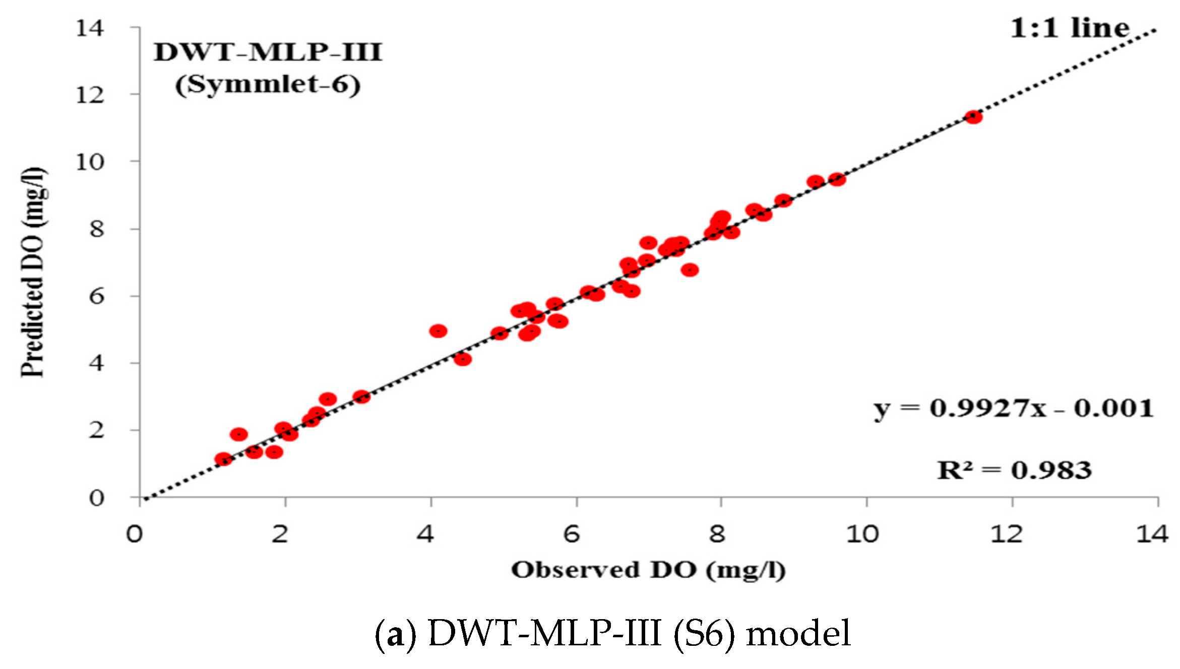
| MLP-III | C6 | 9-27-1 | 0.523 | 0.958 | 0.989 | 0.958 | 0.345 | 0.364 | 0.978 | 0.994 | 0.978 | 0.291 |
| C12 | 9-26-1 | 0.418 | 0.974 | 0.993 | 0.974 | 0.314 | 0.178 | 0.979 | 0.995 | 0.979 | 0.066 | |
| C18 | 9-21-1 | 0.441 | 0.971 | 0.992 | 0.971 | 0.343 | 0.202 | 0.973 | 0.993 | 0.975 | 0.072 | |
| D6 | 9-22-1 | 0.437 | 0.971 | 0.993 | 0.971 | 0.310 | 0.161 | 0.983 | 0.996 | 0.983 | 0.061 | |
| D12 | 9-22-1 | 0.346 | 0.982 | 0.995 | 0.982 | 0.255 | 0.180 | 0.978 | 0.995 | 0.979 | 0.066 | |
| D18 | 9-28-1 | 0.447 | 0.970 | 0.992 | 0.970 | 0.336 | 0.223 | 0.967 | 0.992 | 0.970 | 0.086 | |
| S6 | 9-22-1 | 0.437 | 0.971 | 0.993 | 0.971 | 0.310 | 0.161 | 0.983 | 0.996 | 0.983 | 0.061 | |
| S12 | 9-28-1 | 0.420 | 0.973 | 0.993 | 0.973 | 0.308 | 0.184 | 0.977 | 0.994 | 0.977 | 0.069 | |
| S18 | 9-37-1 | 0.434 | 0.971 | 0.993 | 0.972 | 0.294 | 0.186 | 0.977 | 0.994 | 0.977 | 0.068 | |
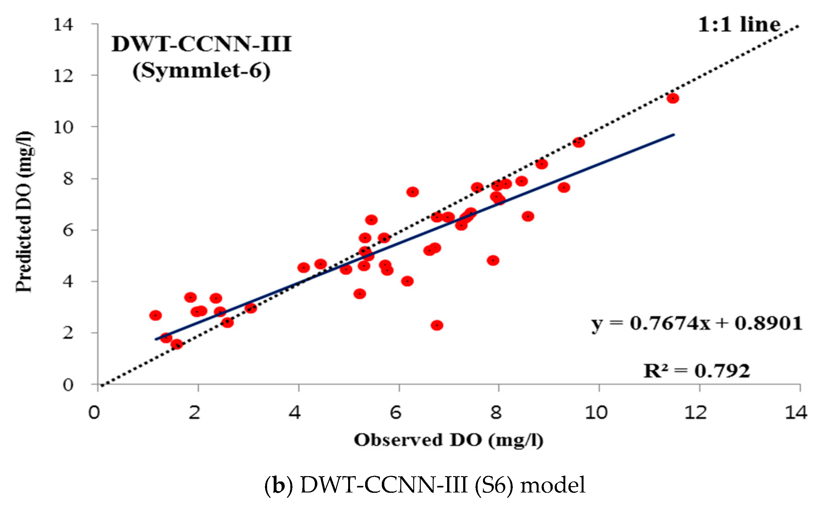
| CCNN-III | C6 | 9-0-1 | 1.341 | 0.727 | 0.914 | 0.730 | 1.035 | 1.360 | 0.693 | 0.907 | 0.739 | 1.055 |
| C12 | 9-0-1 | 1.335 | 0.730 | 0.916 | 0.735 | 1.041 | 0.656 | 0.711 | 0.913 | 0.747 | 0.250 | |
| C18 | 9-1-1 | 1.217 | 0.776 | 0.935 | 0.780 | 0.942 | 0.611 | 0.749 | 0.927 | 0.794 | 0.219 | |
| D6 | 9-2-1 | 1.216 | 0.776 | 0.934 | 0.778 | 0.956 | 0.605 | 0.754 | 0.928 | 0.792 | 0.219 | |
| D12 | 9-1-1 | 1.245 | 0.765 | 0.929 | 0.768 | 0.971 | 0.659 | 0.708 | 0.918 | 0.757 | 0.244 | |
| D18 | 9-0-1 | 1.330 | 0.732 | 0.917 | 0.735 | 1.028 | 0.869 | 0.709 | 0.912 | 0.755 | 0.245 | |
| S6 | 9-2-1 | 1.216 | 0.776 | 0.934 | 0.778 | 0.956 | 0.605 | 0.754 | 0.928 | 0.792 | 0.219 | |
| S12 | 9-0-1 | 1.336 | 0.730 | 0.915 | 0.734 | 1.046 | 0.683 | 0.687 | 0.903 | 0.728 | 0.258 | |
| S18 | 9-1-1 | 1.256 | 0.761 | 0.929 | 0.763 | 0.958 | 0.612 | 0.749 | 0.928 | 0.787 | 0.207 | |
| Model | VMD | Topology | Training Phase | Testing Phase | ||||||||
|---|---|---|---|---|---|---|---|---|---|---|---|---|
| RMSE (mg/L) | NSE | WI | R2 | MAE (mg/L) | RMSE (mg/L) | NSE | WI | R2 | MAE (mg/L) | |||
| MLP-III | K = 3, α = 5 | 9-22-1 | 0.354 | 0.981 | 0.995 | 0.981 | 0.270 | 0.359 | 0.979 | 0.995 | 0.979 | 0.280 |
| K = 4, α = 5 | 12-25-1 | 0.335 | 0.983 | 0.996 | 0.983 | 0.240 | 0.146 | 0.986 | 0.996 | 0.986 | 0.054 | |
| K = 4, α = 10 | 12-19-1 | 0.257 | 0.990 | 0.997 | 0.990 | 0.191 | 0.107 | 0.992 | 0.998 | 0.993 | 0.034 | |
| CCNN-III | K = 3, α = 5 | 9-0-1 | 1.312 | 0.739 | 0.920 | 0.744 | 1.003 | 1.307 | 0.717 | 0.916 | 0.762 | 0.965 |
| K = 4, α = 5 | 12-0-1 | 1.322 | 0.735 | 0.921 | 0.737 | 1.026 | 0.611 | 0.750 | 0.926 | 0.792 | 0.228 | |
| K = 4, α = 10 | 12-0-1 | 1.327 | 0.733 | 0.921 | 0.738 | 1.036 | 0.597 | 0.761 | 0.929 | 0.791 | 0.218 | |
© 2019 by the authors. Licensee MDPI, Basel, Switzerland. This article is an open access article distributed under the terms and conditions of the Creative Commons Attribution (CC BY) license (http://creativecommons.org/licenses/by/4.0/).
Share and Cite
Zounemat-Kermani, M.; Seo, Y.; Kim, S.; Ghorbani, M.A.; Samadianfard, S.; Naghshara, S.; Kim, N.W.; Singh, V.P. Can Decomposition Approaches Always Enhance Soft Computing Models? Predicting the Dissolved Oxygen Concentration in the St. Johns River, Florida. Appl. Sci. 2019, 9, 2534. https://doi.org/10.3390/app9122534
Zounemat-Kermani M, Seo Y, Kim S, Ghorbani MA, Samadianfard S, Naghshara S, Kim NW, Singh VP. Can Decomposition Approaches Always Enhance Soft Computing Models? Predicting the Dissolved Oxygen Concentration in the St. Johns River, Florida. Applied Sciences. 2019; 9(12):2534. https://doi.org/10.3390/app9122534
Chicago/Turabian StyleZounemat-Kermani, Mohammad, Youngmin Seo, Sungwon Kim, Mohammad Ali Ghorbani, Saeed Samadianfard, Shabnam Naghshara, Nam Won Kim, and Vijay P. Singh. 2019. "Can Decomposition Approaches Always Enhance Soft Computing Models? Predicting the Dissolved Oxygen Concentration in the St. Johns River, Florida" Applied Sciences 9, no. 12: 2534. https://doi.org/10.3390/app9122534