An Elastic Interface Model for the Delamination of Bending-Extension Coupled Laminates

Abstract

The paper addresses the problem of an interfacial crack in a multi-directional laminated beam with possible bending-extension coupling. A crack-tip element is considered as an assemblage of two sublaminates connected by an elastic-brittle interface of negligible thickness. Each sublaminate is modeled as an extensible, flexible, and shear-deformable laminated beam. The mathematical problem is reduced to a set of two differential equations in the interfacial stresses. Explicit expressions are derived for the internal forces, strain measures, and generalized displacements in the sublaminates. Then, the energy release rate and its Mode I and Mode II contributions are evaluated. As an example, the model is applied to the analysis of the double cantilever beam test with both symmetric and asymmetric laminated specimens.

1. Introduction

Delamination, or interlaminar fracture, is the main life-limiting failure mode for fiber-reinforced composite laminates [1]. Delamination cracks may originate from localized defects and propagate due to peak interlaminar stresses. A huge number of analytical, numerical, and experimental studies have been devoted to this problem during the last few decades [2,3,4,5,6]. The phenomenon is also relevant for many similar layered structures, such as glued laminated timber beams [7] and multilayered ceramic composites [8].

Within the framework of linear elastic fracture mechanics (LEFM), a delamination crack is expected to propagate when the energy release rate, $\mathcal{G}$, attains a critical value, or fracture toughness, ${\mathcal{G}}_{\mathrm{c}}$. Since delamination cracks preferentially propagate along the weak interfaces between adjoining plies (laminae), propagation generally involves a mix of the three basic fracture modes (Mode I or opening, Mode II or sliding, and Mode III or tearing). Each fracture mode furnishes an additive contribution to the total energy release rate, ${\mathcal{G}}_{\mathrm{I}}$, ${\mathcal{G}}_{\mathrm{II}}$, and ${\mathcal{G}}_{\mathrm{III}}$[9], and corresponds to a different value of interlaminar fracture toughness, ${\mathcal{G}}_{\mathrm{Ic}}$, ${\mathcal{G}}_{\mathrm{IIc}}$, and ${\mathcal{G}}_{\mathrm{IIIc}}$ [10]. Thus, to predict delamination crack propagation, it is necessary (i) to assess by experiments the interlaminar fracture toughness (in pure and mixed fracture modes), (ii) to define a suitable mixed-mode fracture criterion, and (iii) to use a theoretical model to evaluate the energy release rate and its modal contributions [11].

An effective modeling approach to evaluate the energy release rate is to consider a delaminated laminate as composed of sublaminates connected by an elastic interface, i.e., a continuous distribution of linearly elastic–brittle springs. Such an elastic interface model was developed first by Kanninen for the double cantilever beam (DCB) test specimen [12] and later adopted by many authors for the analysis of the delamination of composite laminates [13,14,15,16,17,18,19,20,21,22,23,24,25,26]. Elastic interface models can be regarded as particular cases of the more general cohesive-zone models [27,28]. The latter are increasingly used to model delamination associated with large-scale bridging and other non-linear damage phenomena [29,30,31,32,33,34,35,36,37,38]. A parallel line of research concerns adhesively-bonded joints, for which models of growing complexity have been proposed in the literature [39]: from elastic interface models [40,41,42,43,44,45,46] to non-linear cohesive-zone models [47,48].

Bending-extension coupling and other elastic couplings are a typical feature of composite laminated beams and plates [49]. Nevertheless, only a few theoretical models for the study of delamination take into account elastic couplings. Among these, it is worth citing the pioneering work by Schapery and Davidson on the prediction of the energy release rate in mixed-mode fracture conditions [50]. In recent years, Xie et al. considered bending-extension coupling in the analysis of delamination toughness specimens [36] and composite laminated plates subjected to flexural loading [25]. Dimitri et al. presented a general formulation of the elastic interface model including bending-extension and shear deformability, but limited their analytical solution to the case with no elastic coupling [26]. Valvo analyzed the delamination of shear-deformable laminated beams with bending-extension coupling based on a rigid interface model [51]. Tsokanas and Loutas extended the above-mentioned analysis to include the effects of crack tip rotations and hygrothermal stresses [52]. To the best of our knowledge, a complete analytical solution for the elastic interface model of delaminated beams with bending-extension coupling and shear deformability has not yet been presented in the literature.

This paper analyses the problem of an interfacial crack in a multi-directional laminated beam with possible bending-extension coupling [53]. A crack-tip element is defined as a laminate segment extending ahead and behind the crack tip cross-section, such that the fracture process zone is fully included within [54,55]. In line with the elastic interface modeling approach, the crack-tip element is considered as an assemblage of two sublaminates connected by an elastic-brittle interface of negligible thickness. Each sublaminate is modeled as an extensible, flexible, and shear-deformable laminated beam [56]. The mathematical problem is reduced to a set of two differential equations in the interfacial stresses. A complete analytical solution is derived including explicit expressions for the internal forces, strain measures, and generalized displacements in the sublaminates. Then, the energy release rate and its Mode I and Mode II contributions are evaluated based on Rice’s $\mathcal{J}$-integral [57]. By way of illustration, the model is applied to the analysis of the DCB test. Three laminated specimens are analyzed, made up of uni-directional, cross-ply, and multi-directional sublaminates.

2. Crack-Tip Element

2.1. Mechanical Model

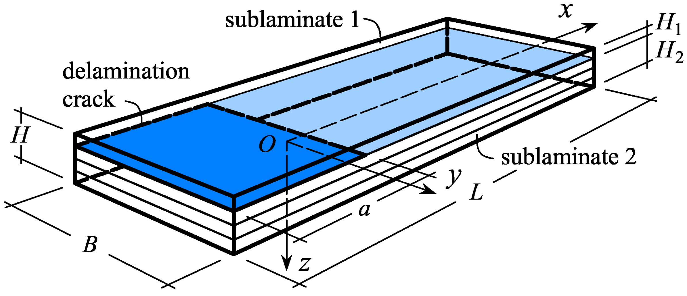
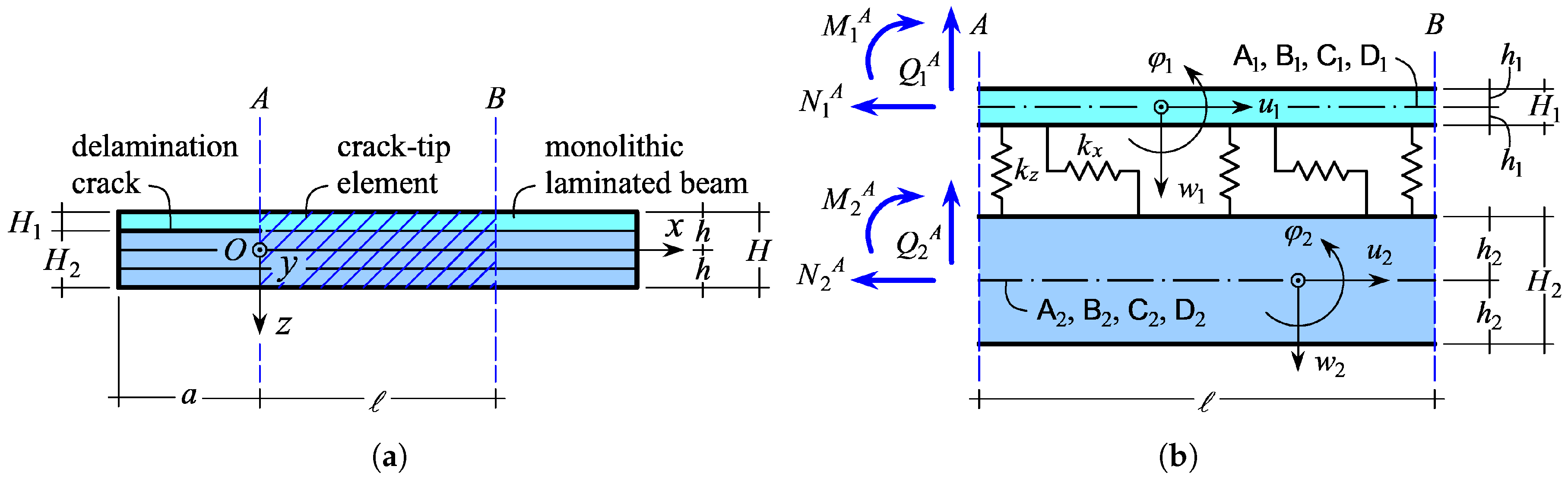
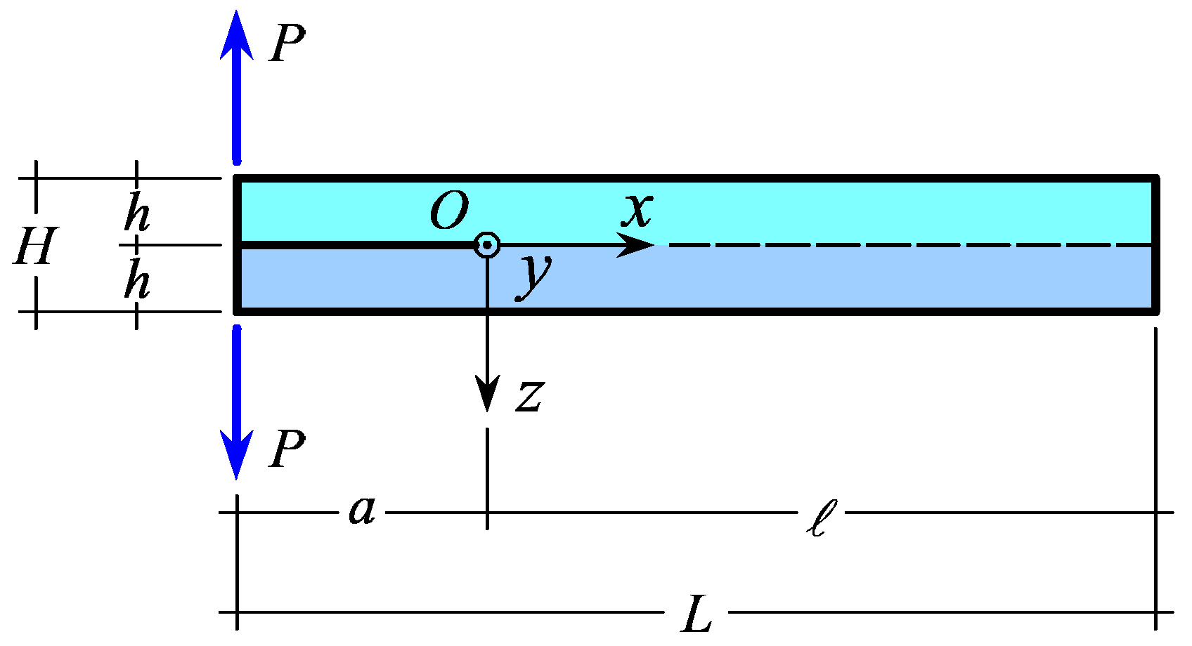
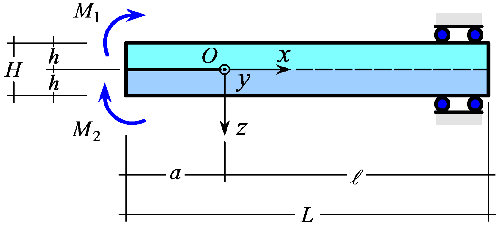
Let us consider a composite laminated beam of length L, width B, and thickness $H=2h$, with a through-the-width delamination crack of length a. The delamination plane ideally subdivides the laminate into two sublaminates (labeled 1 and 2) of thicknesses $H_1=2h_1$ and $H_2=2h_2$. We fix a right-handed global Cartesian reference system, $Oxyz$, with the origin O at the center of the crack tip cross-section and the x-, y-, and z-axes aligned with the laminate longitudinal, width, and thickness directions, respectively (Figure 1).

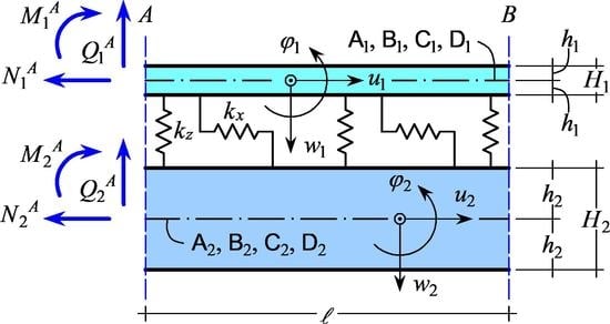
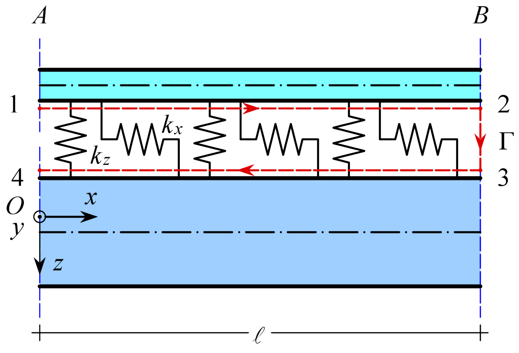
The present mechanical model focuses on a crack-tip element (CTE), here defined as a laminate segment of length ℓ, extending ahead and behind the crack tip cross-section, which fully includes the fracture process zone [54,55]. In practice, the end sections of the CTE, A and B, should be chosen such that A is immediately ahead of the delamination front and B is sufficiently far from it to make sure that the laminate behind behaves as a monolithic beam (Figure 2a). We model the sublaminates as two plane beams connected by an elastic-brittle interface of negligible thickness. The generalized displacements for the sublaminates are defined as follows: $u_{\alpha }$ and $w_{\alpha }$ denote the sublaminate mid-plane displacements along the x- and z-directions, respectively; ${\phi }_{\alpha }$ denote their cross-section rotations about the y-axis (positive if counter-clockwise). Henceforth, the subscript $\alpha$ is used to refer to the upper ($\alpha =1$) and lower ($\alpha =2$) sublaminates (Figure 2b).

In line with the kinematics of Timoshenko’s beam theory [56], we define the strain measures for the sublaminates as the mid-plane axial strain, ${ϵ}_{\alpha }$, average shear strain, ${\gamma }_{\alpha }$, and pseudo-curvature, ${\kappa }_{\alpha }$. These are related to the generalized displacements as follows:

$${ϵ}_{\alpha }=\frac{\mathrm{d}{u}_{\alpha }}{\mathrm{d}x},{\gamma }_{\alpha }=\frac{\mathrm{d}{w}_{\alpha }}{\mathrm{d}x}+{\phi }_{\alpha },\mathrm{and}{\kappa }_{\alpha }=\frac{\mathrm{d}{\phi }_{\alpha }}{\mathrm{d}x}.$$

(1)

Next, we introduce the conjugated internal forces, namely the axial force, $N_{\alpha }$, shear force, $Q_{\alpha }$, and bending moment, $M_{\alpha }$. For a laminated beam with bending-extension coupling, the internal forces are related to the strain measures as follows:

$$N_{\alpha }={\mathsf{A}}_{\alpha }{ϵ}_{\alpha }+{\mathsf{B}}_{\alpha }{\kappa }_{\alpha },Q_{\alpha }={\mathsf{C}}_{\alpha }{\gamma }_{\alpha },\mathrm{and}{M}_{\alpha }={\mathsf{B}}_{\alpha }{ϵ}_{\alpha }+{\mathsf{D}}_{\alpha }{\kappa }_{\alpha },$$

(2)

where ${\mathsf{A}}_{\alpha }$, ${\mathsf{B}}_{\alpha }$, ${\mathsf{C}}_{\alpha }$, and ${\mathsf{D}}_{\alpha }$ respectively denote the sublaminate extensional stiffness, bending-extension coupling stiffness, shear stiffness, and bending stiffness. In general, such stiffnesses should be calculated according to classical laminated plate theory [49], as detailed in Appendix A.

For what follows, it is convenient to introduce also the sublaminate compliances,

$${\mathsf{a}}_{\alpha }=\frac{{\mathsf{D}}_{\alpha }}{{\mathsf{A}}_{\alpha }{\mathsf{D}}_{\alpha }-{{\mathsf{B}}_{\alpha }}^2},{\mathsf{b}}_{\alpha }=-\frac{{\mathsf{B}}_{\alpha }}{{\mathsf{A}}_{\alpha }{\mathsf{D}}_{\alpha }-{{\mathsf{B}}_{\alpha }}^2},{\mathsf{c}}_{\alpha }=\frac{1}{{\mathsf{C}}_{\alpha }},\mathrm{and}{\mathsf{d}}_{\alpha }=\frac{{\mathsf{A}}_{\alpha }}{{\mathsf{A}}_{\alpha }{\mathsf{D}}_{\alpha }-{{\mathsf{B}}_{\alpha }}^2},$$

(3)

and write the constitutive relations, Equation (2), in inverse form:

$${ϵ}_{\alpha }={\mathsf{a}}_{\alpha }{N}_{\alpha }+{\mathsf{b}}_{\alpha }{M}_{\alpha },{\gamma }_{\alpha }={\mathsf{c}}_{\alpha }{Q}_{\alpha },\mathrm{and}{\kappa }_{\alpha }={\mathsf{b}}_{\alpha }{N}_{\alpha }+{\mathsf{d}}_{\alpha }{M}_{\alpha }.$$

(4)

The elastic interface between the upper and lower sublaminates transfers both normal and shear interfacial stresses, respectively given by:

$$\sigma =k_z\Delta w\mathrm{and}\tau =k_x\Delta u,$$

(5)

where $k_z$ and $k_x$ are the interface elastic constants and:

$$\Delta w=w_2-w_1\mathrm{and}\Delta u=u_2-u_1-{\phi }_2{h}_2-{\phi }_1{h}_1$$

(6)

are the transverse and longitudinal relative displacements at the interface, respectively. By substituting Equation (6) into (5), we obtain:

$$\sigma =k_z\left(w_2-w_1\right)\mathrm{and}\tau =k_x\left(u_2-u_1-{\phi }_2{h}_2-{\phi }_1{h}_1\right).$$

(7)

2.2. Differential Problem

The equilibrium equations for the upper and lower sublaminates are:

$$\frac{\mathrm{d}{N}_{\alpha }}{\mathrm{d}x}+n_{\alpha }=0,\frac{\mathrm{d}{Q}_{\alpha }}{\mathrm{d}x}+q_{\alpha }=0,\mathrm{and}\frac{\mathrm{d}{M}_{\alpha }}{\mathrm{d}x}+m_{\alpha }-Q_{\alpha }=0,$$

(8)

where $n_{\alpha }$, $q_{\alpha }$, and $m_{\alpha }$ respectively are the distributed axial load, transverse load, and bending couple, due to the normal and shear stresses transferred by the interface:

$$n_1=-n_2=B\tau ,q_1=-q_2=B\sigma ,\mathrm{and}{m}_{\alpha }=B\tau h_{\alpha }.$$

(9)

We substitute Equation (9) into (8) and differentiate the latter with respect to x. Then, by using Equations (1)–(4), we obtain the set of governing differential equations for the upper sublaminate,

$$\begin{array}{c}\frac{1}{B}\frac{{\mathrm{d}}^3{u}_1}{\mathrm{d}{x}^3}=-\left({\mathsf{a}}_1+{\mathsf{b}}_1{h}_1\right)\frac{\mathrm{d}\tau }{\mathrm{d}x}-{\mathsf{b}}_1\sigma ,\hfill \\ \frac{1}{B}\frac{{\mathrm{d}}^4{w}_1}{\mathrm{d}{x}^4}=\left({\mathsf{b}}_1+{\mathsf{d}}_1{h}_1\right)\frac{\mathrm{d}\tau }{\mathrm{d}x}-{\mathsf{c}}_1\frac{{\mathrm{d}}^2\sigma }{\mathrm{d}{x}^2}+{\mathsf{d}}_1\sigma ,\mathrm{and}\hfill \\ \frac{1}{B}\frac{{\mathrm{d}}^3{\phi }_1}{\mathrm{d}{x}^3}=-\left({\mathsf{b}}_1+{\mathsf{d}}_1{h}_1\right)\frac{\mathrm{d}\tau }{\mathrm{d}x}-{\mathsf{d}}_1\sigma ,\hfill \end{array}$$

(10)

and for the lower sublaminate,

$$\begin{array}{c}\frac{1}{B}\frac{{\mathrm{d}}^3{u}_2}{\mathrm{d}{x}^3}=\left({\mathsf{a}}_2-{\mathsf{b}}_2{h}_2\right)\frac{\mathrm{d}\tau }{\mathrm{d}x}+{\mathsf{b}}_2\sigma ,\hfill \\ \frac{1}{B}\frac{{\mathrm{d}}^4{w}_2}{\mathrm{d}{x}^4}=-\left({\mathsf{b}}_2-{\mathsf{d}}_2{h}_2\right)\frac{\mathrm{d}\tau }{\mathrm{d}x}+{\mathsf{c}}_2\frac{{\mathrm{d}}^2\sigma }{\mathrm{d}{x}^2}-{\mathsf{d}}_2\sigma ,\mathrm{and}\hfill \\ \frac{1}{B}\frac{{\mathrm{d}}^3{\phi }_2}{\mathrm{d}{x}^3}=\left({\mathsf{b}}_2-{\mathsf{d}}_2{h}_2\right)\frac{\mathrm{d}\tau }{\mathrm{d}x}+{\mathsf{d}}_2\sigma .\hfill \end{array}$$

(11)

2.3. Boundary Conditions

The crack-tip element is subjected to known internal forces on the upper and lower sublaminates at cross-section A. Hence, the following six static boundary conditions can be written:

$$\begin{array}{c}{\left.N_1\right|}_{x=0}=N_1^A,{\left.Q_1\right|}_{x=0}=Q_1^A,{\left.M_1\right|}_{x=0}=M_1^A;\hfill \\ {\left.N_2\right|}_{x=0}=N_2^A,{\left.Q_2\right|}_{x=0}=Q_2^A,{\left.M_2\right|}_{x=0}=M_2^A.\hfill \end{array}$$

(12)

At cross-section B, three kinematic boundary conditions can be obtained from the assumption that the laminate behind behaves as a monolithic beam:

$$\begin{array}{c}{\left.{ϵ}_1\right|}_{x=\ell }+{\left.{\kappa }_1\right|}_{x=\ell }{h}_1={\left.{ϵ}_2\right|}_{x=\ell }-{\left.{\kappa }_2\right|}_{x=\ell }{h}_2,\hfill \\ {\left.{\gamma }_1\right|}_{x=\ell }={\left.{\gamma }_2\right|}_{x=\ell },\mathrm{and}{\left.{\kappa }_1\right|}_{x=\ell }={\left.{\kappa }_2\right|}_{x=\ell }.\hfill \end{array}$$

(13)

To sum up, we have nine boundary conditions to complete the formulation of the differential problem. We note that, in general, no restraints are given to prevent rigid-body motions of the CTE.

3. Solution of the Differential Problem

3.1. Solution Strategy

Following a solution strategy already adopted to solve some specific problems [22,43,44,53], the interfacial stresses are here assumed as the main unknowns. To this aim, we differentiate the normal and shear interfacial stresses, Equation (7), four and three times, respectively, with respect to x. Then, we substitute Equations (10) and (11) into the result. After some simplifications, we obtain the following differential equation set:

$$\begin{array}{c}\frac{{\mathrm{d}}^4\sigma }{\mathrm{d}{x}^4}-{\alpha }_1\frac{{\mathrm{d}}^2\sigma }{\mathrm{d}{x}^2}+{\alpha }_2\sigma +k_z{\beta }_0\frac{\mathrm{d}\tau }{\mathrm{d}x}=0,\hfill \\ \frac{{\mathrm{d}}^3\tau }{\mathrm{d}{x}^3}-{\alpha }_3\frac{\mathrm{d}\tau }{\mathrm{d}x}-k_x{\beta }_0\sigma =0,\hfill \end{array}$$

(14)

where:

$$\begin{array}{c}{\alpha }_1=k_{z}B\left({\mathsf{c}}_1+{\mathsf{c}}_2\right),{\alpha }_2=k_{z}B\left({\mathsf{d}}_1+{\mathsf{d}}_2\right),\mathrm{and}\hfill \\ {\alpha }_3=k_{x}B\left({\mathsf{a}}_1+{\mathsf{a}}_2+2{\mathsf{b}}_1{h}_1-2{\mathsf{b}}_2{h}_2+{\mathsf{d}}_1{h_1}^2+{\mathsf{d}}_2{h_2}^2\right)\hfill \end{array}$$

(15)

are constant coefficients and:

$${\beta }_0=B\left({\mathsf{b}}_1+{\mathsf{b}}_2+{\mathsf{d}}_1{h}_1-{\mathsf{d}}_2{h}_2\right)$$

(16)

is a coupling parameter, here called the unbalance parameter by analogy with the literature on adhesive joints [39].

Two cases have to be considered in solving the differential problem:

(1) the balanced case, when ${\beta }_0=0$, i.e., ${\mathsf{d}}_1{h}_1+{\mathsf{b}}_1={\mathsf{d}}_2{h}_2-{\mathsf{b}}_2$. This condition is trivially fulfilled, for instance, by homogeneous laminates with mid-plane delaminations (for which ${\mathsf{b}}_1={\mathsf{b}}_2=0$, ${\mathsf{d}}_1={\mathsf{d}}_2$, and $h_1=h_2$) or symmetrically-stacked laminates with mid-plane delaminations (for which ${\mathsf{b}}_1=-{\mathsf{b}}_2$, ${\mathsf{d}}_1={\mathsf{d}}_2$, and $h_1=h_2$). Besides, the balance condition is satisfied by homogeneous sublaminates with bending stiffness ratio $\frac{{\mathsf{D}}_{\mathsf{1}}}{{\mathsf{D}}_{\mathsf{2}}}=\frac{h_1}{h_2}$ [38,58]. More generally, it is possible to conceive of non-trivial stacking sequences, where the upper and lower sublaminates have unequal thicknesses, but fulfil the balance condition [59,60]. In the balanced case, Equations (14) are uncoupled and can be solved separately to obtain the normal and shear interfacial stresses;

(2) the unbalanced case, when ${\beta }_0\ne 0$, i.e., ${\mathsf{d}}_1{h}_1+{\mathsf{b}}_1\ne {\mathsf{d}}_2{h}_2-{\mathsf{b}}_2$. This condition corresponds to laminates with generic stacking sequences and arbitrarily-located delaminations (with respect to the mid-plane). In the unbalanced case, Equations (14) are coupled and must be solved simultaneously.

In the following subsections, we will show how to solve the stated differential problem and obtain the expressions for the interfacial stresses. Then, by using Equations (1), (4) and (8), it is straightforward to deduce also the expressions for the internal forces, strain measures, and generalized displacements.

3.2. Balanced Case

3.2.1. Interfacial Stresses

In the balanced case, the differential problem, Equation (14), reduces to the following two uncoupled differential equations:

$$\begin{array}{c}\frac{{\mathrm{d}}^4\sigma }{\mathrm{d}{x}^4}-{\alpha }_1\frac{{\mathrm{d}}^2\sigma }{\mathrm{d}{x}^2}+{\alpha }_2\sigma =0,\hfill \\ \frac{{\mathrm{d}}^3\tau }{\mathrm{d}{x}^3}-{\alpha }_3\frac{\mathrm{d}\tau }{\mathrm{d}x}=0,\hfill \end{array}$$

(17)

whose coefficients are defined in Equation (15).

The general solution for the interfacial stresses in the balanced case can be written as follows:

$$\begin{array}{c}\sigma \left(x\right)=\frac{1}{B}\sum _{i=1}^4{f}_{i}exp\left(-{\lambda }_{i}x\right),\hfill \\ \tau \left(x\right)=\frac{1}{B}\left[f_{5}exp\left(-{\lambda }_{5}x\right)+f_{6}exp\left(-{\lambda }_{6}x\right)+f_7\right],\hfill \end{array}$$

(18)

where $f_1$, $f_2$, …, $f_7$ are integration constants and:

$$\begin{array}{c}{\lambda }_1=\frac{1}{\sqrt{2}}\sqrt{{\alpha }_1-\sqrt{{\alpha }_1^2-4{\alpha }_2}},{\lambda }_2=-{\lambda }_1,\hfill \\ {\lambda }_3=\frac{1}{\sqrt{2}}\sqrt{{\alpha }_1+\sqrt{{\alpha }_1^2-4{\alpha }_2}},{\lambda }_4=-{\lambda }_3,\hfill \\ {\lambda }_5=\sqrt{{\alpha }_3},\mathrm{and}{\lambda }_6=-{\lambda }_5\hfill \end{array}$$

(19)

are the non-zero roots of the characteristic equation of the differential problem (17):

$$\left({\lambda }^4-{\alpha }_1{\lambda }^2+{\alpha }_2\right)\left({\lambda }^2-{\alpha }_3\right)=0.$$

(20)

Strictly speaking, the solution expressed by Equation (18) holds provided that the interface constant $k_z$ is not equal to the following “critical” value:

$${\widehat{k}}_z=\frac{4}{B}\frac{{\mathsf{d}}_1+{\mathsf{d}}_2}{{\left({\mathsf{c}}_1+{\mathsf{c}}_2\right)}^2},$$

(21)

for which Equation (20) has coincident roots and the solution requires a different expression. However, for material properties corresponding to common fiber-reinforced laminates, the numerical values of $k_z$ are usually greater than ${\widehat{k}}_z$, and the roots of the characteristic equation are real-valued (see Appendix B.1). For very compliant interfaces, e.g., if the present model is applied to the analysis of adhesively-bonded joints with weak adhesive, it may happen that $k_z<{\widehat{k}}_z$, and the characteristic equation has complex roots. In such cases, the present solution is still valid, provided that the complex exponential functions are considered in Equation (18) and the following. Similar considerations apply also to the unbalanced case.

3.2.2. Internal Forces

By substituting Equation (18) into (9), the latter into (8), and integrating with respect to x, we obtain the expressions for the internal forces in the upper sublaminate,

$$\begin{array}{cc}\hfill N_1\left(x\right)=& \frac{f_5}{{\lambda }_5}exp\left(-{\lambda }_{5}x\right)+\frac{f_6}{{\lambda }_6}exp\left(-{\lambda }_{6}x\right)-f_{7}x-f_8,\hfill \\ \hfill Q_1\left(x\right)=& \sum _{i=1}^4\frac{f_i}{{\lambda }_i}exp\left(-{\lambda }_{i}x\right)-f_{10},\mathrm{and}\hfill \\ \hfill M_1\left(x\right)=& -\sum _{i=1}^4\frac{f_i}{{\lambda }_i^2}exp\left(-{\lambda }_{i}x\right)+\frac{h_1{f}_5}{{\lambda }_5}exp\left(-{\lambda }_{5}x\right)+\frac{h_1{f}_6}{{\lambda }_6}exp\left(-{\lambda }_{6}x\right)-\left(f_{10}+h_1{f}_7\right)x-f_{12},\hfill \end{array}$$

(22)

and in the lower sublaminate,

$$\begin{array}{c}{N}_2\left(x\right)=-\frac{f_5}{{\lambda }_5}exp\left(-{\lambda }_{5}x\right)-\frac{f_6}{{\lambda }_6}exp\left(-{\lambda }_{6}x\right)+f_{7}x+f_9,\hfill \\ Q_2\left(x\right)=-\sum _{i=1}^4\frac{f_i}{{\lambda }_i}exp\left(-{\lambda }_{i}x\right)+f_{11},\mathrm{and}\hfill \\ M_2\left(x\right)=\sum _{i=1}^4\frac{f_i}{{\lambda }_i^2}exp\left(-{\lambda }_{i}x\right)+\frac{h_2{f}_5}{{\lambda }_5}exp\left(-{\lambda }_{5}x\right)+\frac{h_2{f}_6}{{\lambda }_6}exp\left(-{\lambda }_{6}x\right)+\left(f_{11}-h_2{f}_7\right)x+f_{13},\hfill \end{array}$$

(23)

where $f_8$, $f_9$, …, $f_{13}$ are integration constants.

3.2.3. Strain Measures

By substituting Equations (22) and (23) into (4), we obtain the expressions for the strain measures in the upper sublaminate,

$$\begin{array}{cc}\hfill {ϵ}_1\left(x\right)=& \left({\mathsf{a}}_1+{\mathsf{b}}_1{h}_1\right)\left[\frac{f_5}{{\lambda }_5}exp\left(-{\lambda }_{5}x\right)+\frac{f_6}{{\lambda }_6}exp\left(-{\lambda }_{6}x\right)\right]-{\mathsf{b}}_1\sum _{i=1}^4\frac{f_i}{{\lambda }_i^2}exp\left(-{\lambda }_{i}x\right)+\hfill \\ & -\left[\left({\mathsf{a}}_1+{\mathsf{b}}_1{h}_1\right)f_7+{\mathsf{b}}_1{f}_{10}\right]x-{\mathsf{a}}_1{f}_8-{\mathsf{b}}_1{f}_{12},\hfill \\ \hfill {\gamma }_1\left(x\right)=& {\mathsf{c}}_1\sum _{i=1}^4\frac{f_i}{{\lambda }_i}exp\left(-{\lambda }_{i}x\right)-{\mathsf{c}}_1{f}_{10},\mathrm{and}\hfill \\ \hfill {\kappa }_1\left(x\right)=& -{\mathsf{d}}_1\sum _{i=1}^4\frac{f_i}{{\lambda }_i^2}exp\left(-{\lambda }_{i}x\right)+\left({\mathsf{d}}_1{h}_1+{\mathsf{b}}_1\right)\left[\frac{f_5}{{\lambda }_5}exp\left(-{\lambda }_{5}x\right)+\frac{f_6}{{\lambda }_6}exp\left(-{\lambda }_{6}x\right)\right]+\hfill \\ & -\left[\left({\mathsf{d}}_1{h}_1+{\mathsf{b}}_1\right)f_7+{\mathsf{d}}_1{f}_{10}\right]x-{\mathsf{b}}_1{f}_8-{\mathsf{d}}_1{f}_{12},\hfill \end{array}$$

(24)

and in the lower sublaminate,

$$\begin{array}{cc}\hfill {ϵ}_2\left(x\right)=& -\left({\mathsf{a}}_2-{\mathsf{b}}_2{h}_2\right)\left[\frac{f_5}{{\lambda }_5}exp\left(-{\lambda }_{5}x\right)+\frac{f_6}{{\lambda }_6}exp\left(-{\lambda }_{6}x\right)\right]+{\mathsf{b}}_2\sum _{i=1}^4\frac{f_i}{{\lambda }_i^2}exp\left(-{\lambda }_{i}x\right)+\hfill \\ & +\left[\left({\mathsf{a}}_2-{\mathsf{b}}_2{h}_2\right)f_7+{\mathsf{b}}_2{f}_{11}\right]x+{\mathsf{a}}_2{f}_9+{\mathsf{b}}_2{f}_{13},\hfill \\ \hfill {\gamma }_2\left(x\right)=& -{\mathsf{c}}_2\sum _{i=1}^4\frac{f_i}{{\lambda }_i}exp\left(-{\lambda }_{i}x\right)+{\mathsf{c}}_2{f}_{11},\mathrm{and}\hfill \\ \hfill {\kappa }_2\left(x\right)=& {\mathsf{d}}_2\sum _{i=1}^4\frac{f_i}{{\lambda }_i^2}exp\left(-{\lambda }_{i}x\right)+\left({\mathsf{d}}_2{h}_2-{\mathsf{b}}_2\right)\left[\frac{f_5}{{\lambda }_5}exp\left(-{\lambda }_{5}x\right)+\frac{f_6}{{\lambda }_6}exp\left(-{\lambda }_{6}x\right)\right]+\hfill \\ & -\left[\left({\mathsf{d}}_2{h}_2-{\mathsf{b}}_2\right)f_7-{\mathsf{d}}_2{f}_{11}\right]x+{\mathsf{b}}_2{f}_9+{\mathsf{d}}_2{f}_{13}.\hfill \end{array}$$

(25)

3.2.4. Generalized Displacements

Lastly, by substituting Equations (24) and (25) into (1) and integrating the latter with respect to x, we obtain the expressions for the generalized displacements in the upper sublaminate,

$$\begin{array}{cc}\hfill u_1\left(x\right)=& -\left({\mathsf{a}}_1+{\mathsf{b}}_1{h}_1\right)\left[\frac{f_5}{{\lambda }_5^2}exp\left(-{\lambda }_{5}x\right)+\frac{f_6}{{\lambda }_6^2}exp\left(-{\lambda }_{6}x\right)\right]+{\mathsf{b}}_1\sum _{i=1}^4\frac{f_i}{{\lambda }_i^3}exp\left(-{\lambda }_{i}x\right)+\hfill \\ & -\left[\left({\mathsf{a}}_1+{\mathsf{b}}_1{h}_1\right)f_7+{\mathsf{b}}_1{f}_{10}\right]\frac{x^2}{2}-\left({\mathsf{a}}_1{f}_8+{\mathsf{b}}_1{f}_{12}\right)x+f_{14},\hfill \\ \hfill w_1\left(x\right)=& \sum _{i=1}^4\left(\frac{{\mathsf{d}}_1}{{\lambda }_i^2}-{\mathsf{c}}_1\right)\frac{f_i}{{\lambda }_i^2}exp\left(-{\lambda }_{i}x\right)-\left({\mathsf{d}}_1{h}_1+{\mathsf{b}}_1\right)\left[\frac{f_5}{{\lambda }_5^3}exp\left(-{\lambda }_{5}x\right)+\frac{f_6}{{\lambda }_6^3}exp\left(-{\lambda }_{6}x\right)\right]+\hfill \\ & +\left[\left({\mathsf{d}}_1{h}_1+{\mathsf{b}}_1\right)f_7+{\mathsf{d}}_1{f}_{10}\right]\frac{x^3}{6}+\left({\mathsf{b}}_1{f}_8+{\mathsf{d}}_1{f}_{12}\right)\frac{x^2}{2}-\left(f_{16}+{\mathsf{c}}_1{f}_{10}\right)x+f_{15},\mathrm{and}\hfill \\ \hfill {\phi }_1\left(x\right)=& {\mathsf{d}}_1\sum _{i=1}^4\frac{f_i}{{\lambda }_i^3}exp\left(-{\lambda }_{i}x\right)-\left({\mathsf{d}}_1{h}_1+{\mathsf{b}}_1\right)\left[\frac{f_5}{{\lambda }_5^2}exp\left(-{\lambda }_{5}x\right)+\frac{f_6}{{\lambda }_6^2}exp\left(-{\lambda }_{6}x\right)\right]+\hfill \\ & -\left[\left({\mathsf{d}}_1{h}_1+{\mathsf{b}}_1\right)f_7+{\mathsf{d}}_1{f}_{10}\right]\frac{x^2}{2}-\left({\mathsf{b}}_1{f}_8+{\mathsf{d}}_1{f}_{12}\right)x+f_{16},\hfill \end{array}$$

(26)

and in the lower sublaminate,

$$\begin{array}{cc}\hfill u_2\left(x\right)=& \left({\mathsf{a}}_2-{\mathsf{b}}_2{h}_2\right)\left[\frac{f_5}{{\lambda }_5^2}exp\left(-{\lambda }_{5}x\right)+\frac{f_6}{{\lambda }_6^2}exp\left(-{\lambda }_{6}x\right)\right]-{\mathsf{b}}_2\sum _{i=1}^4\frac{f_i}{{\lambda }_i^3}exp\left(-{\lambda }_{i}x\right)+\hfill \\ & +\left[\left({\mathsf{a}}_2-{\mathsf{b}}_2{h}_2\right)f_7+{\mathsf{b}}_2{f}_{11}\right]\frac{x^2}{2}+\left({\mathsf{a}}_2{f}_9+{\mathsf{b}}_2{f}_{13}\right)x+f_{17},\hfill \\ \hfill w_2\left(x\right)=& -\sum _{i=1}^4\left(\frac{{\mathsf{d}}_2}{{\lambda }_i^2}-{\mathsf{c}}_2\right)\frac{f_i}{{\lambda }_i^2}exp\left(-{\lambda }_{i}x\right)-\left({\mathsf{d}}_2{h}_2-{\mathsf{b}}_2\right)\left[\frac{f_5}{{\lambda }_5^3}exp\left(-{\lambda }_{5}x\right)+\frac{f_6}{{\lambda }_6^3}exp\left(-{\lambda }_{6}x\right)\right]+\hfill \\ & +\left[\left({\mathsf{d}}_2{h}_2-{\mathsf{b}}_2\right)f_7-{\mathsf{d}}_2{f}_{11}\right]\frac{x^3}{6}-\left({\mathsf{b}}_2{f}_9+{\mathsf{d}}_2{f}_{13}\right)\frac{x^2}{2}-\left(f_{19}-{\mathsf{c}}_2{f}_{11}\right)x+f_{18},\mathrm{and}\hfill \\ \hfill {\phi }_2\left(x\right)=& -{\mathsf{d}}_2\sum _{i=1}^4\frac{f_i}{{\lambda }_i^3}exp\left(-{\lambda }_{i}x\right)-\left({\mathsf{d}}_2{h}_2-{\mathsf{b}}_2\right)\left[\frac{f_5}{{\lambda }_5^2}exp\left(-{\lambda }_{5}x\right)+\frac{f_6}{{\lambda }_6^2}exp\left(-{\lambda }_{6}x\right)\right]+\hfill \\ & -\left[\left({\mathsf{d}}_2{h}_2-{\mathsf{b}}_2\right)f_7-{\mathsf{d}}_2{f}_{11}\right]\frac{x^2}{2}+\left({\mathsf{b}}_2{f}_9+{\mathsf{d}}_2{f}_{13}\right)x+f_{19},\hfill \end{array}$$

(27)

where $f_{14}$, $f_{15}$, …, $f_{19}$ are further integration constants.

3.2.5. Supernumerary Integration Constants

In the obtained analytical solution, nineteen integration constants appear. However, seven of them are supernumerary as a consequence of the adopted solution strategy (see Section 3.1). To determine the supernumerary integration constants, we substitute the solution for the interfacial stresses, Equation (18), and generalized displacements, Equations (26) and (27), into Equation (7). In this way, two identities are obtained, which need to be fulfilled for all values of x. The following seven relations among the integration constants are determined:

$$\begin{array}{c}{f}_{10}=-\frac{{\alpha }_3}{B{k}_x{\alpha }_4}{\mathsf{d}}_2{f}_7,f_{11}=\frac{{\alpha }_3}{B{k}_x{\alpha }_4}{\mathsf{d}}_1{f}_7,\hfill \\ f_{12}=-\frac{\left({\mathsf{a}}_1+{\mathsf{b}}_1{h}_1\right){\mathsf{d}}_2-\left({\mathsf{b}}_2-{\mathsf{d}}_2{h}_2\right){\mathsf{b}}_1}{{\alpha }_4}{f}_8-\frac{{\mathsf{a}}_2{\mathsf{d}}_2-{\mathsf{b}}_2^2}{{\alpha }_4}{f}_9,\hfill \\ f_{13}=\frac{{\mathsf{a}}_1{\mathsf{d}}_1-{\mathsf{b}}_1^2}{{\alpha }_4}{f}_8+\frac{\left({\mathsf{a}}_2-{\mathsf{b}}_2{h}_2\right){\mathsf{d}}_1-\left({\mathsf{b}}_1+{\mathsf{d}}_1{h}_1\right){\mathsf{b}}_2}{{\alpha }_4}{f}_9,\hfill \\ f_{14}=f_{17}-\left(h_1+h_2\right)f_{19}-\frac{1}{k_x}\left[\frac{1}{B}+\frac{{\alpha }_3}{B{\alpha }_4}\left({\mathsf{c}}_1{\mathsf{d}}_2-{\mathsf{c}}_2{\mathsf{d}}_1\right)h_1\right]f_7,\hfill \\ f_{15}=f_{18},\mathrm{and}{f}_{16}=f_{19}+\frac{{\alpha }_3}{B{k}_x{\alpha }_4}\left({\mathsf{c}}_1{\mathsf{d}}_2-{\mathsf{c}}_2{\mathsf{d}}_1\right)f_7,\hfill \end{array}$$

(28)

where:

$${\alpha }_4={\mathsf{b}}_1{\mathsf{d}}_2-{\mathsf{b}}_2{\mathsf{d}}_1+{\mathsf{d}}_1{\mathsf{d}}_2(h_1+h_2).$$

(29)

The values of the remaining twelve independent integration constants ($f_1$, $f_2$, …, $f_9$ and $f_{17}$, $f_{18}$, and $f_{19}$) have to be determined by imposing the boundary conditions of the particular problem being solved. It can be noted that the last three independent integration constants describe a rigid motion of the specimen and can be assessed only when appropriate kinematic restraints are prescribed. The adopted solution strategy enables the determination of the internal forces, strain measures, and relative displacements, even though the values of the last three constants remain undetermined.

3.3. Unbalanced Case

3.3.1. Interfacial Stresses

In the unbalanced case, Equations (14) are coupled. To separate the unknowns, we solve the first of such equations w.r.t. to $\mathrm{d}\tau /\mathrm{d}x$ and substitute the result into the second equation. After some simplifications, we obtain:

$$\begin{array}{c}\frac{{\mathrm{d}}^6\sigma }{\mathrm{d}{x}^6}-{\beta }_1\frac{{\mathrm{d}}^4\sigma }{\mathrm{d}{x}^4}+{\beta }_2\frac{{\mathrm{d}}^2\sigma }{\mathrm{d}{x}^2}-{\beta }_3\sigma =0,\hfill \\ \frac{\mathrm{d}\tau }{\mathrm{d}x}=-\frac{1}{k_z{\beta }_0}\left(\frac{{\mathrm{d}}^4\sigma }{\mathrm{d}{x}^4}-{\alpha }_1\frac{{\mathrm{d}}^2\sigma }{\mathrm{d}{x}^2}+{\alpha }_2\sigma \right),\hfill \end{array}$$

(30)

where:

$${\beta }_1={\alpha }_1+{\alpha }_3,{\beta }_2={\alpha }_2+{\alpha }_1{\alpha }_3,\mathrm{and}{\beta }_3={\alpha }_2{\alpha }_3-k_x{k}_z{\beta }_0^2,$$

(31)

with ${\alpha }_1$, ${\alpha }_2$, ${\alpha }_3$, and ${\beta }_0$ already defined in Equations (15) and (16), respectively.

The general solution for the interfacial stresses in the unbalanced case can be written as follows:

$$\begin{array}{c}\sigma \left(x\right)=\frac{1}{B}\sum _{i=1}^6{g}_{i}exp\left(-{\mu }_{i}x\right),\hfill \\ \tau \left(x\right)=-\frac{k_x{\beta }_0}{B}\sum _{i=1}^6\frac{g_{i}exp\left(-{\mu }_{i}x\right)}{{\mu }_i\left({\mu }_i^2-{\alpha }_3\right)}+\frac{g_7}{B},\hfill \end{array}$$

(32)

where $g_1$, $g_2$, …, $g_7$ are integration constants and ${\mu }_1$, ${\mu }_2$, …, ${\mu }_6$ are the non-zero roots of the characteristic equation of the differential problem (30):

$${\mu }^6-{\beta }_1{\mu }^4+{\beta }_2{\mu }^2-{\beta }_3=0.$$

(33)

By substituting Equation (31) into (33), the latter can be rearranged as:

$$\left({\mu }^2-{\lambda }_1^2\right)\left({\mu }^2-{\lambda }_3^2\right)\left({\mu }^2-{\lambda }_5^2\right)+k_x{k}_z{\beta }_0^2=0,$$

(34)

where ${\lambda }_1$, ${\lambda }_3$, and ${\lambda }_5$ are given by Equation (19). From Equation (34), it can be easily concluded that the roots of the characteristic equation for the unbalanced case are different from those for the balanced case. Conversely, by assuming ${\beta }_0=0$, Equation (34) turns out to be equivalent to Equation (20).

In general, Equation (33) can be solved numerically. In Appendix B.2, the conditions are given for which ${\mu }_1$, ${\mu }_2$, …, ${\mu }_6$ are real, along with their analytical expressions in this case. It should be noted that, strictly speaking, the solution expressed by Equation (32) is valid only when the characteristic equation has no coincident roots, which is the case for common geometric and material properties.

3.3.2. Internal Forces

By substituting Equation (32) into (9), the latter into (8), and integrating with respect to x, we obtain the expressions for the internal forces in the upper sublaminate,

$$\begin{array}{cc}\hfill N_1\left(x\right)=& -k_x{\beta }_0\sum _{i=1}^6\frac{g_i}{{\mu }_i^2\left({\mu }_i^2-{\alpha }_3\right)}exp\left(-{\mu }_{i}x\right)-g_{7}x-g_8,\hfill \\ \hfill Q_1\left(x\right)=& \sum _{i=1}^6\frac{g_i}{{\mu }_i}exp\left(-{\mu }_{i}x\right)-g_{10},\mathrm{and}\hfill \\ \hfill M_1\left(x\right)=& -\sum _{i=1}^6\frac{g_i}{{\mu }_i^2}\left(1+\frac{h_1{k}_x{\beta }_0}{{\mu }_i^2-{\alpha }_3}\right)exp\left(-{\mu }_{i}x\right)-\left(h_1{g}_7+g_{10}\right)x-g_{12},\hfill \end{array}$$

(35)

and in the lower sublaminate,

$$\begin{array}{cc}\hfill N_2\left(x\right)=& k_x{\beta }_0\sum _{i=1}^6\frac{g_i}{{\mu }_i^2\left({\mu }_i^2-{\alpha }_3\right)}exp\left(-{\mu }_{i}x\right)+g_{7}x+g_9,\hfill \\ \hfill Q_2\left(x\right)=& -\sum _{i=1}^6\frac{g_i}{{\mu }_i}exp\left(-{\mu }_{i}x\right)+g_{11},\mathrm{and}\hfill \\ \hfill M_2\left(x\right)=& \sum _{i=1}^6\frac{g_i}{{\mu }_i^2}\left(1-\frac{h_2{k}_x{\beta }_0}{{\mu }_i^2-{\alpha }_3}\right)exp\left(-{\mu }_{i}x\right)-\left(h_2{g}_7-g_{11}\right)x+g_{13},\hfill \end{array}$$

(36)

where $g_8$, $g_9$, …, $g_{13}$ are integration constants.

3.3.3. Strain Measures

By substituting Equations (35) and (36) into (4), we obtain the expressions for the strain measures in the upper sublaminate,

$$\begin{array}{cc}\hfill {ϵ}_1\left(x\right)=& -\sum _{i=1}^6\frac{g_i}{{\mu }_i^2}\left[\frac{k_x{\beta }_0}{{\mu }_i^2-{\alpha }_3}\left({\mathsf{a}}_1+{\mathsf{b}}_1{h}_1\right)+{\mathsf{b}}_1\right]exp\left(-{\mu }_{i}x\right)+\hfill \\ & -\left[\left({\mathsf{a}}_1+{\mathsf{b}}_1{h}_1\right)g_7+{\mathsf{b}}_1{g}_{10}\right]x-{\mathsf{a}}_1{g}_8-{\mathsf{b}}_1{g}_{12},\hfill \\ \hfill {\gamma }_1\left(x\right)=& {\mathsf{c}}_1\sum _{i=1}^6\frac{g_i}{{\mu }_i}exp\left(-{\mu }_{i}x\right)-{\mathsf{c}}_1{g}_{10},\mathrm{and}\hfill \\ \hfill {\kappa }_1\left(x\right)=& -\sum _{i=1}^6\frac{g_i}{{\mu }_i^2}\left[{\mathsf{d}}_1+\frac{k_x{\beta }_0}{{\mu }_i^2-{\alpha }_3}\left({\mathsf{d}}_1{h}_1+{\mathsf{b}}_1\right)\right]exp\left(-{\mu }_{i}x\right)+\hfill \\ & -\left[\left({\mathsf{d}}_1{h}_1+{\mathsf{b}}_1\right)g_7+{\mathsf{d}}_1{g}_{10}\right]x-{\mathsf{b}}_1{g}_8-{\mathsf{d}}_1{g}_{12},\hfill \end{array}$$

(37)

and in the lower sublaminate,

$$\begin{array}{cc}\hfill {ϵ}_2\left(x\right)=& \sum _{i=1}^6\frac{g_i}{{\mu }_i^2}\left[\frac{k_x{\beta }_0}{{\mu }_i^2-{\alpha }_3}\left({\mathsf{a}}_2-{\mathsf{b}}_2{h}_2\right)+{\mathsf{b}}_2\right]exp\left(-{\mu }_{i}x\right)+\hfill \\ & +\left[\left({\mathsf{a}}_2-{\mathsf{b}}_2{h}_2\right)g_7+{\mathsf{b}}_2{g}_{11}\right]x+{\mathsf{a}}_2{g}_9+{\mathsf{b}}_2{g}_{13},\hfill \\ \hfill {\gamma }_2\left(x\right)=& -{\mathsf{c}}_2\sum _{i=1}^6\frac{g_i}{{\mu }_i}exp\left(-{\mu }_{i}x\right)+{\mathsf{c}}_2{g}_{11},\mathrm{and}\hfill \\ \hfill {\kappa }_2\left(x\right)=& \sum _{i=1}^6\frac{g_i}{{\mu }_i^2}\left[{\mathsf{d}}_2-\frac{k_x{\beta }_0}{{\mu }_i^2-{\alpha }_3}\left({\mathsf{d}}_2{h}_2-{\mathsf{b}}_2\right)\right]exp\left(-{\mu }_{i}x\right)+\hfill \\ & -\left[\left({\mathsf{d}}_2{h}_2-{\mathsf{b}}_2\right)g_7-{\mathsf{d}}_2{g}_{11}\right]x+{\mathsf{b}}_2{g}_9+{\mathsf{d}}_2{g}_{13}.\hfill \end{array}$$

(38)

3.3.4. Generalized Displacements

Lastly, by substituting Equations (37) and (38) into (1) and integrating the latter with respect to x, we obtain the expressions for the generalized displacements in the upper sublaminate,

$$\begin{array}{cc}\hfill u_1\left(x\right)=& \sum _{i=1}^6\frac{g_i}{{\mu }_i^3}\left[\frac{k_x{\beta }_0}{{\mu }_i^2-{\alpha }_3}\left({\mathsf{a}}_1+{\mathsf{b}}_1{h}_1\right)+{\mathsf{b}}_1\right]exp\left(-{\mu }_{i}x\right)+\hfill \\ & -\left[\left({\mathsf{a}}_1+{\mathsf{b}}_1{h}_1\right)g_7+{\mathsf{b}}_1{g}_{10}\right]\frac{x^2}{2}-\left({\mathsf{a}}_1{g}_8+{\mathsf{b}}_1{g}_{12}\right)x+g_{14},\hfill \\ \hfill w_1\left(x\right)=& \sum _{i=1}^6\frac{g_i}{{\mu }_i^2}\left[\frac{{\mathsf{d}}_1}{{\mu }_i^2}-{\mathsf{c}}_1+\frac{k_x{\beta }_0\left({\mathsf{d}}_1{h}_1+{\mathsf{b}}_1\right)}{{\mu }_i^2\left({\mu }_i^2-{\alpha }_3\right)}\right]exp\left(-{\mu }_{i}x\right)+\hfill \\ & +\left[\left({\mathsf{d}}_1{h}_1+{\mathsf{b}}_1\right)g_7+{\mathsf{d}}_1{g}_{10}\right]\frac{x^3}{6}+\left({\mathsf{b}}_1{g}_8+{\mathsf{d}}_1{g}_{12}\right)\frac{x^2}{2}-\left({\mathsf{c}}_1{g}_{10}+g_{16}\right)x+g_{15},\mathrm{and}\hfill \\ \hfill {\phi }_1\left(x\right)=& \sum _{i=1}^6\frac{g_i}{{\mu }_i^3}\left[\frac{k_x{\beta }_0}{{\mu }_i^2-{\alpha }_3}\left({\mathsf{d}}_1{h}_1+{\mathsf{b}}_1\right)+{\mathsf{d}}_1\right]exp\left(-{\mu }_{i}x\right)+\hfill \\ & -\left[\left({\mathsf{d}}_1{h}_1+{\mathsf{b}}_1\right)g_7+{\mathsf{d}}_1{g}_{10}\right]\frac{x^2}{2}-\left({\mathsf{b}}_1{g}_8+{\mathsf{d}}_1{g}_{12}\right)x+g_{16},\hfill \end{array}$$

(39)

and in the lower sublaminate,

$$\begin{array}{cc}\hfill u_2\left(x\right)=& -\sum _{i=1}^6\frac{g_i}{{\mu }_i^3}\left[\frac{k_x{\beta }_0}{{\mu }_i^2-{\alpha }_3}\left({\mathsf{a}}_2-{\mathsf{b}}_2{h}_2\right)+{\mathsf{b}}_2\right]exp\left(-{\mu }_{i}x\right)+\hfill \\ & +\left[\left({\mathsf{a}}_2-{\mathsf{b}}_2{h}_2\right)g_7+{\mathsf{b}}_2{g}_{11}\right]\frac{x^2}{2}+\left({\mathsf{a}}_2{g}_9+{\mathsf{b}}_2{g}_{13}\right)x+g_{17},\hfill \\ \hfill w_2\left(x\right)=& -\sum _{i=1}^6\frac{g_i}{{\mu }_i^2}\left[\frac{{\mathsf{d}}_2}{{\mu }_i^2}-{\mathsf{c}}_2-\frac{k_x{\beta }_0\left({\mathsf{d}}_2{h}_2-{\mathsf{b}}_2\right)}{{\mu }_i^2\left({\mu }_i^2-{\alpha }_3\right)}\right]exp\left(-{\mu }_{i}x\right)+\hfill \\ & +\left[\left({\mathsf{d}}_2{h}_2-{\mathsf{b}}_2\right)g_7-{\mathsf{d}}_2{g}_{11}\right]\frac{x^3}{6}-\left({\mathsf{b}}_2{g}_9+{\mathsf{d}}_2{g}_{13}\right)\frac{x^2}{2}+\left({\mathsf{c}}_2{g}_{11}-g_{19}\right)x+g_{18},\mathrm{and}\hfill \\ \hfill {\phi }_2\left(x\right)=& \sum _{i=1}^6\frac{g_i}{{\mu }_i^3}\left[\frac{k_x{\beta }_0}{{\mu }_i^2-{\alpha }_3}\left({\mathsf{d}}_2{h}_2-{\mathsf{b}}_2\right)-{\mathsf{d}}_2\right]exp\left(-{\mu }_{i}x\right)+\hfill \\ & -\left[\left({\mathsf{d}}_2{h}_2-{\mathsf{b}}_2\right)g_7-{\mathsf{d}}_2{g}_{11}\right]\frac{x^2}{2}+\left({\mathsf{b}}_2{g}_9+{\mathsf{d}}_2{g}_{13}\right)x+g_{19},\hfill \end{array}$$

(40)

where $g_{14}$, $g_{15}$, …, $g_{19}$ are further integration constants.

3.3.5. Supernumerary Integration Constants

As for the balanced case (see Section 3.2.5), nineteen integration constants appear in the analytical solution for the unbalanced case. Again, seven of them are supernumerary and can be determined by substituting the solution for the interfacial stresses, Equation (32), and generalized displacements, Equations (39) and (40), into Equation (7). In this way, two identities are obtained, which need to be fulfilled for all values of x. Consequently, the following seven relations among the integration constants are determined:

$$\begin{array}{c}{g}_{10}=\left(-\frac{{\alpha }_3}{B{k}_x{\alpha }_4}{\mathsf{d}}_2+{\beta }_0\frac{{\mathsf{b}}_2-{\mathsf{d}}_2{h}_2}{{B\alpha }_4}\right)g_7,g_{11}=\left(\frac{{\alpha }_3}{B{k}_x{\alpha }_4}{\mathsf{d}}_1-{\beta }_0\frac{{\mathsf{b}}_1+{\mathsf{d}}_1{h}_1}{{B\alpha }_4}\right)g_7,\hfill \\ g_{12}=-\frac{\left({\mathsf{a}}_1+{\mathsf{b}}_1{h}_1\right){\mathsf{d}}_2-\left({\mathsf{b}}_2-{\mathsf{d}}_2{h}_2\right){\mathsf{b}}_1}{{\alpha }_4}{g}_8-\frac{{\mathsf{a}}_2{\mathsf{d}}_2-{\mathsf{b}}_2^2}{{\alpha }_4}{g}_9,\hfill \\ g_{13}=\frac{{\mathsf{a}}_1{\mathsf{d}}_1-{\mathsf{b}}_1^2}{{\alpha }_4}{g}_8+\frac{\left({\mathsf{a}}_2-{\mathsf{b}}_2{h}_2\right){\mathsf{d}}_1-\left({\mathsf{b}}_1+{\mathsf{d}}_1{h}_1\right){\mathsf{b}}_2}{{\alpha }_4}{g}_9,\hfill \\ g_{14}=g_{17}-\left(h_1+h_2\right)g_{19}-\left[\frac{1}{B{k}_x}+\frac{{\alpha }_3}{{Bk}_x{\alpha }_4}\left({\mathsf{c}}_1{\mathsf{d}}_2-{\mathsf{c}}_2{\mathsf{d}}_1\right)h_1+{\beta }_0\frac{{\mathsf{b}}_1{\mathsf{c}}_2-{\mathsf{c}}_1{\mathsf{b}}_2+{\mathsf{c}}_1{\mathsf{d}}_2{h}_2+{\mathsf{c}}_2{\mathsf{d}}_1{h}_1}{{B\alpha }_4}{h}_1\right]g_7,\hfill \\ g_{15}=g_{18},\mathrm{and}{g}_{16}=g_{19}+\left[\frac{{\alpha }_3}{{Bk}_x{\alpha }_4}\left({\mathsf{c}}_1{\mathsf{d}}_2-{\mathsf{c}}_2{\mathsf{d}}_1\right)+{\beta }_0\frac{{\mathsf{b}}_1{\mathsf{c}}_2-{\mathsf{c}}_1{\mathsf{b}}_2+{\mathsf{c}}_1{\mathsf{d}}_2{h}_2+{\mathsf{c}}_2{\mathsf{d}}_1{h}_1}{{B\alpha }_4}\right]g_7,\hfill \end{array}$$

(41)

where ${\alpha }_4$ is furnished by Equation (29).

The values of the remaining twelve independent integration constants ($g_1$, $g_2$, …, $g_9$ and $g_{17}$, $g_{18}$, and $g_{19}$) have to be determined by imposing the boundary conditions of the particular problem being solved. Again, the last three independent integration constants describe a rigid motion of the specimen and can be assessed only when appropriate kinematic restraints are prescribed. The adopted solution strategy enables the determination of internal forces, strain measures, and relative displacements, even though the values of the last three constants remain undetermined.

4. Delamination Crack Analysis

4.1. Energy Release Rate

Under I/II mixed-mode fracture conditions, the energy release rate can be written as $\mathcal{G}={\mathcal{G}}_{\mathrm{I}}+{\mathcal{G}}_{\mathrm{II}}$, where ${\mathcal{G}}_{\mathrm{I}}$ and ${\mathcal{G}}_{\mathrm{II}}$ are the contributions related to Fracture Modes I and II, respectively. In LEFM, the energy release rate identifies the path-independent $\mathcal{J}\text{-}\mathrm{integral}$ introduced by Rice [57]. Choosing an integration path encircling the interface between sublaminates, as detailed in Appendix C, we obtain:

$$\mathcal{J}=\frac{1}{2}{k}_z\Delta w^2\left(0\right)+\frac{1}{2}{k}_x\Delta u^2\left(0\right)$$

(42)

or, by recalling Equation (5),

$$\mathcal{J}=\frac{{\sigma }_0^2}{2k_z}+\frac{{\tau }_0^2}{2k_x},$$

(43)

where ${\sigma }_0=\sigma \left(0\right)$ and ${\tau }_0=\tau \left(0\right)$ are the peak values of the interfacial stresses at the delamination front. The two addends in Equation (43) correspond to the Mode I and Mode II contributions to the energy release rate, respectively [41]. Since compressive normal stresses at the crack tip (${\sigma }_0<0$) do not promote crack opening, the modal contributions to the energy release rate can be written as

$${\mathcal{G}}_{\mathrm{I}}=\mathcal{H}\left({\sigma }_0\right)\frac{{\sigma }_0^2}{2k_z}\mathrm{and}{\mathcal{G}}_{\mathrm{II}}=\frac{{\tau }_0^2}{2k_x},$$

(44)

where $\mathcal{H}\left(·\right)$ denotes the Heaviside step function. By substituting Equation (18) into (44), we obtain the following expressions for the balanced case:

$${\mathcal{G}}_{\mathrm{I}}=\frac{\mathcal{H}\left({\sigma }_0\right)}{2k_z{B}^2}{\left(\sum _{i=1}^4{f}_i\right)}^2\mathrm{and}{\mathcal{G}}_{\mathrm{II}}=\frac{1}{2k_x{B}^2}{\left(f_5+f_6\right)}^2$$

(45)

Likewise, by substituting Equation (32) into (44), we obtain the following expressions for the unbalanced case:

$${\mathcal{G}}_{\mathrm{I}}=\frac{\mathcal{H}\left({\sigma }_0\right)}{2k_z{B}^2}{\left(\sum _{i=1}^6{g}_i\right)}^2\mathrm{and}{\mathcal{G}}_{\mathrm{II}}=\frac{1}{2k_x{B}^2}{\left(k_x{\beta }_0\sum _{i=1}^6\frac{g_i}{{\mu }_i\left({\mu }_i^2-{\alpha }_3\right)}\right)}^2.$$

(46)

Lastly, to characterize the ratio between the modal contributions to the energy release rate, we introduce the mode-mixity angle [11],

$$\psi =sign\left({\tau }_0\right)arctan\sqrt{\frac{{\mathcal{G}}_{\mathrm{II}}}{{\mathcal{G}}_{\mathrm{I}}}},$$

(47)

ranging from 0 (pure Mode I) to 90 (pure Mode II).

5. Results

5.1. Examples

By way of illustration, we applied the developed solution to the analysis of the DCB test (Figure 3). Laminated specimens with the following geometric sizes were considered: $L=100$ mm, $B=25$ mm, and $H=3.2$ mm. A delamination length $a=25$ mm and a reference load $P=100$ N were used in all of the following calculations. Boundary conditions (12) and (13) were specialized to the present case by taking the crack tip internal forces as $N_1^A=N_2^A=0$, $Q_1^A=-Q_2^A=P$, and $M_1^A=-M_2^A=Pa$ and assuming a CTE length $\ell =L-a$.

Three laminated specimens with different stacking sequences were ideally built as follows. We started from a typical carbon-epoxy fiber-reinforced lamina of thickness $t_p=0.2$ mm and elastic moduli shown in

Table 1. Lamina elastic moduli.

${\mathit{E}}_1$	${\mathit{E}}_2={\mathit{E}}_3$	${\mathit{\nu }}_{12}={\mathit{\nu }}_{13}$	${\mathit{\nu }}_{23}$	${\mathit{G}}_{12}={\mathit{G}}_{13}$	${\mathit{G}}_{23}$
(MPa)	(MPa)	–	–	(MPa)	(MPa)
109,000	8819	0.342	0.380	4315	3200

[61]. Based on this, three stacking sequences were designed corresponding to uni-directional (UD), cross-ply (CP), and multi-directional (MD) sublaminates (

Table 2. Sublaminate stacking sequences.

Sublaminate	Stacking Sequence
UD	$[0_8]$
CP	$[0/90/0_2/{90}_3/0]$
MD	$[45/{-45}_2/90/{45}_2/-45/0]$

). Lastly, the DCB test specimens were obtained by variously assembling the sublaminates one over the other:

• UD//UD
• UD//CP
• UD//MD

where the double slash (//) represents the position of the delamination crack.

The sublaminate plate stiffness matrices, calculated as explained in Appendix A, are reported in

Table 3. Sublaminate plate stiffnesses.

Sublaminate		$\left[{\mathit{A}}_{\mathbf{ij}}\right]$			$\left[{\mathit{B}}_{\mathbf{ij}}\right]$			$\left[{\mathit{D}}_{\mathbf{ij}}\right]$
		(N/mm)			(N)			(N mm)
	176,066	4872	0	0	0	0	37,561	1039	0
UD	4872	14,245	0	0	0	0	1039	3039	0
	0	0	6904	0	0	0	0	0	1473
	95,156	4872	0	8091	0	0	25,155	1039	0
CP	4872	95,156	0	0	−8091	0	1039	15,445	0
	0	0	6904	0	0	0	0	0	1473
	66,477	33,550	0	10,959	−2868	0	19,419	6775	0
MD	33,550	66,477	0	−2868	−5223	0	6775	9710	0
	0	0	35,582	0	0	−2868	0	0	7209

. It can be noted that no bending-extension coupling was exhibited by the UD sublaminate (all terms $B_{ij}=0$), while bending-extension coupling was shown by both the CP (terms $B_{xx}=-B_{yy}\ne 0$) and MD sublaminates (all terms $B_{ij}\ne 0$, except $B_{xs}=B_{ys}=0$).

The sublaminate equivalent beam stiffnesses, calculated via Equations (A10) and (A19), are given in

Table 4. Sublaminate equivalent beam stiffnesses.

Sublaminate	$\mathsf{A}$	$\mathsf{B}$	$\mathsf{C}$	$\mathsf{D}$
	(kN)	(kN mm)	(kN)	(kN mm2)
UD	4360.0	0	143.8	930.1
CP	2372.4	201.5	129.0	627.0
MD	1238.5	314.2	123.8	367.0

. It can be noted that the UD sublaminate had the highest extensional and bending stiffnesses, $\mathsf{A}$ and $\mathsf{D}$, while the MD sublaminate had the highest bending-extension coupling stiffness, $\mathsf{B}$. The shear stiffness, $\mathsf{C}$, showed little variations among the chosen stacking sequences.

A crucial point for the successful implementation of the present model is the appropriate choice of the values of the elastic interface constants. These can be assigned by conducting a compliance calibration with experimental tests or numerical simulations, if available [62]. In a previous study on asymmetric DCB test specimens [22], compliance calibration with finite element simulations gave:

$$k_x\approx 16.2\frac{G_{13}}{H}\mathrm{and}{k}_z\approx 6.9\frac{E_3}{H},$$

(48)

which, in the present case, yielded $k_x=$ 21,845 N/mm³ and $k_z=$ 19,016 N/mm³. Such values were adopted for the present examples.

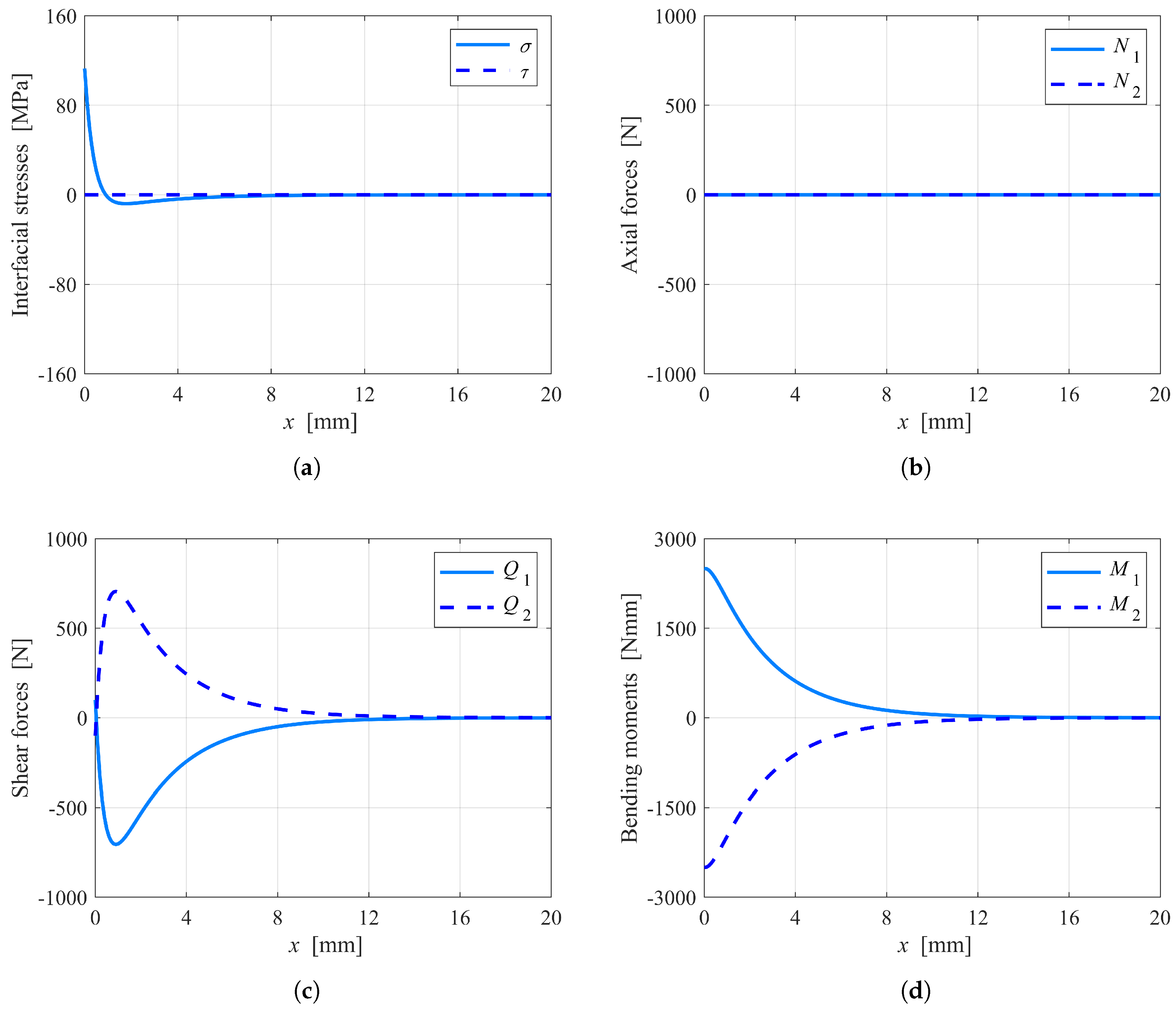
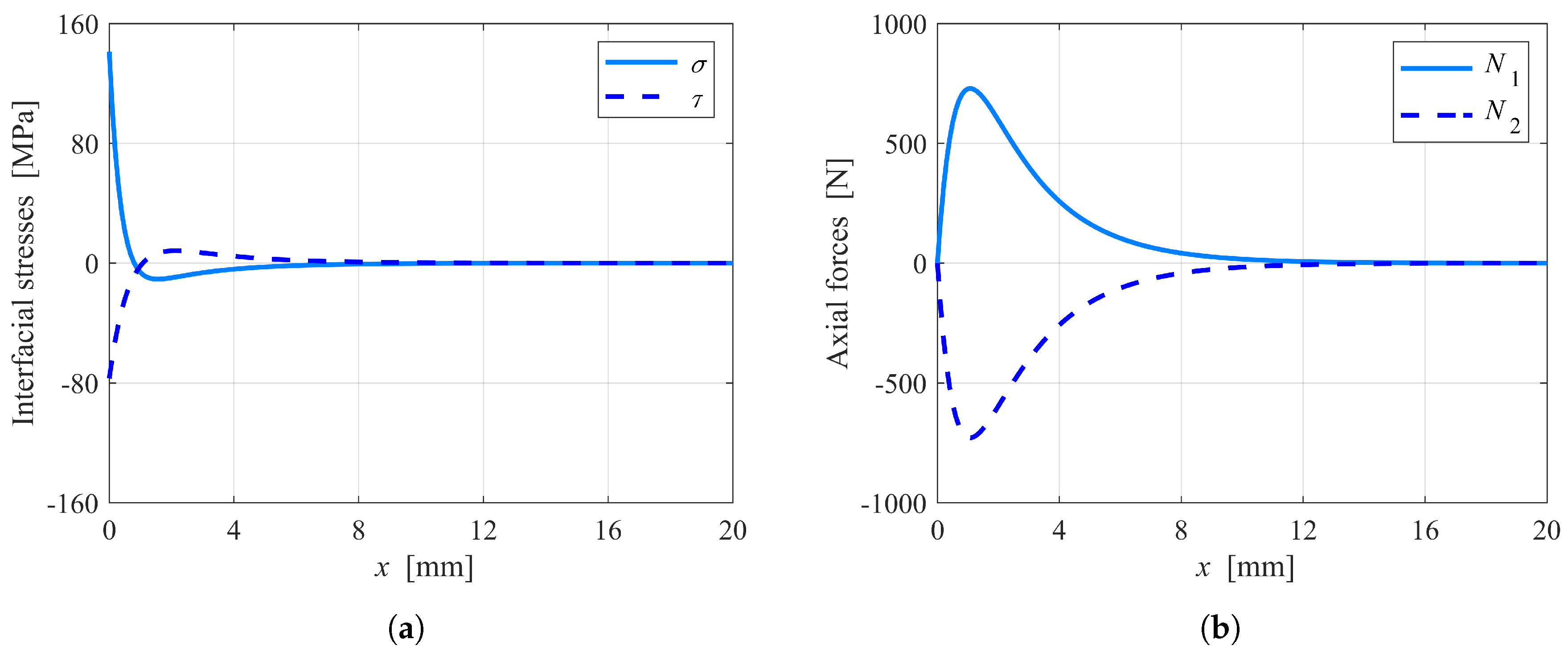
Figure 4 shows the plots of the interfacial stresses and internal forces as functions of the x-coordinate in the neighborhood of the crack tip for the UD//UD specimen. This specimen was symmetric; hence, the unbalance parameter was ${\beta }_0=0$, and the analytical solution for the balanced case applied (see Section 3.2). For the DCB test, the specimen response also corresponded to pure Mode I fracture conditions: actually, Figure 4a shows that the shear stresses were identically null, while the normal stresses attained a peak value at the crack tip cross-section. Figure 4b shows that also the sublaminate axial forces were null. Instead, Figure 4c,d shows the trends of the sublaminate shear forces and bending moments, which started from the assigned values at the crack tip cross-section and then approached zero asymptotically. Shear forces and bending moments had symmetric trends in the upper and lower sublaminates because of the specimen symmetry.

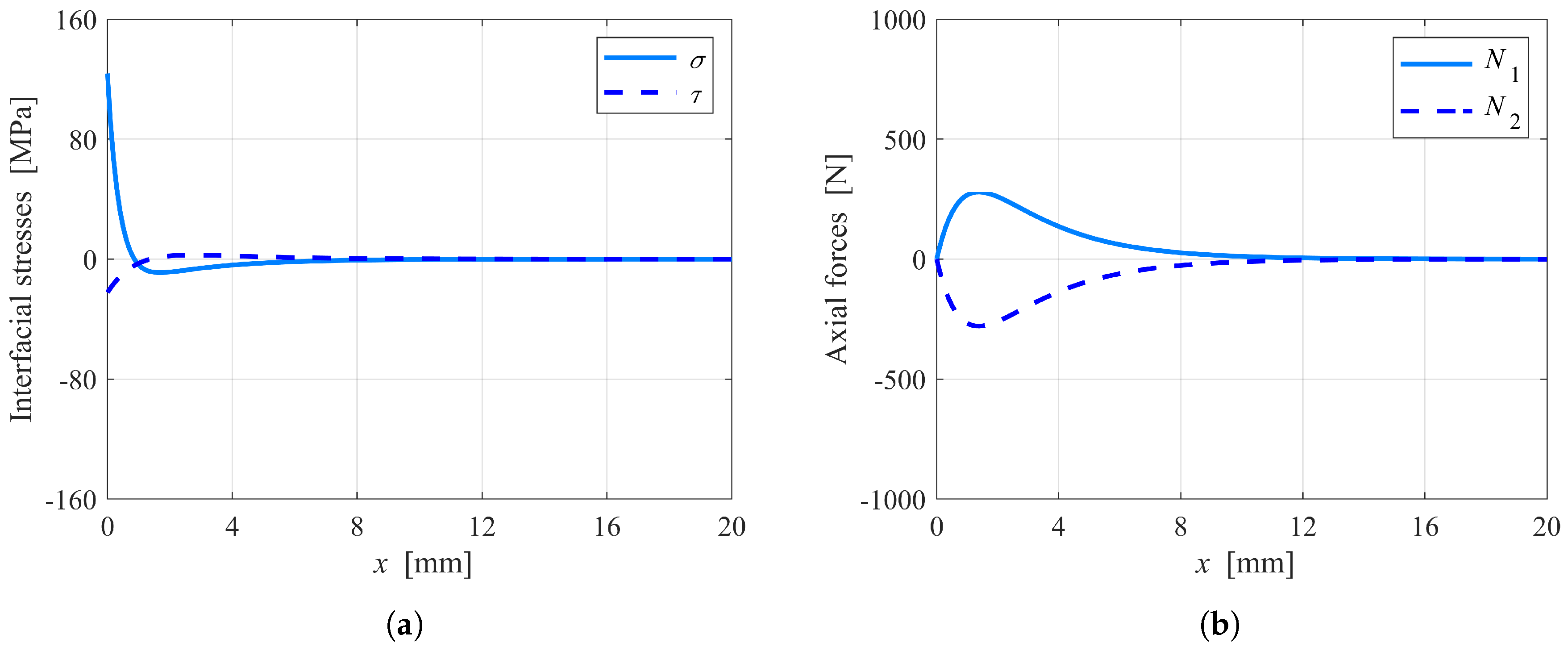
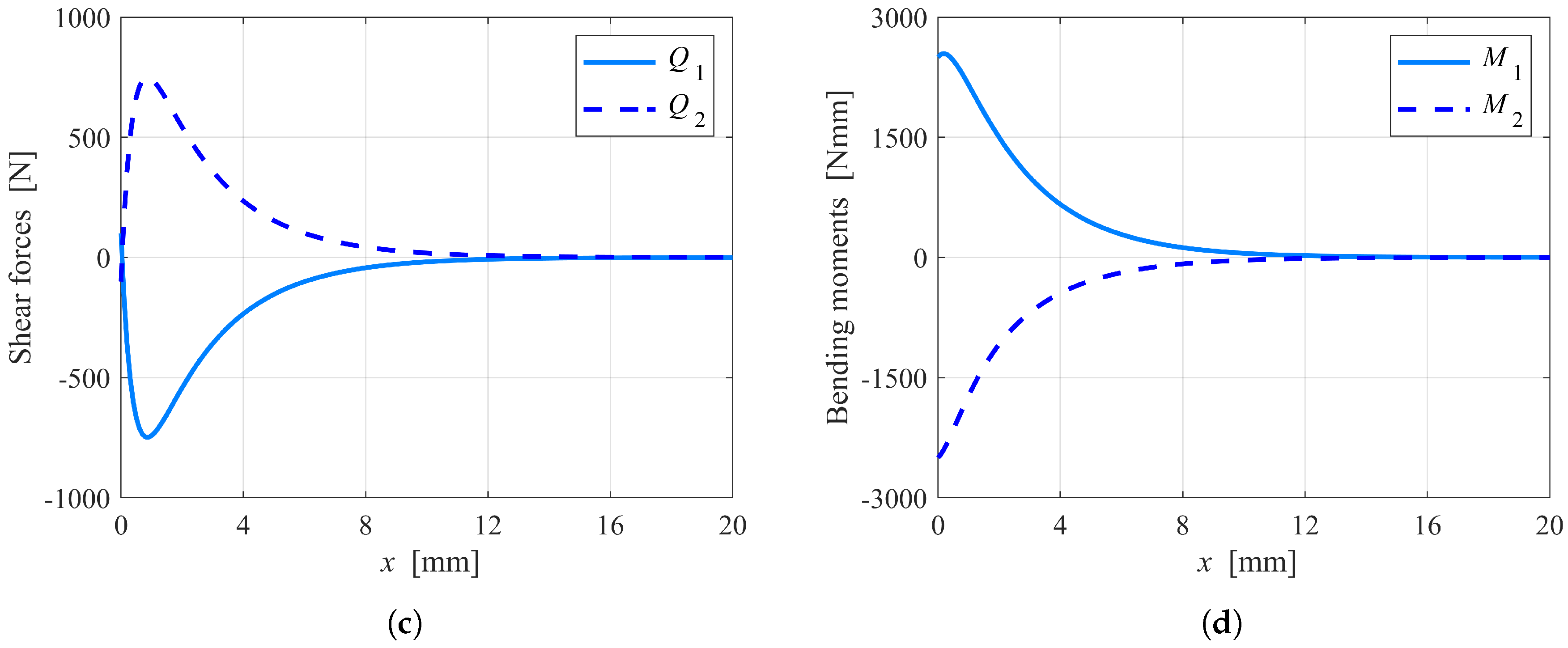
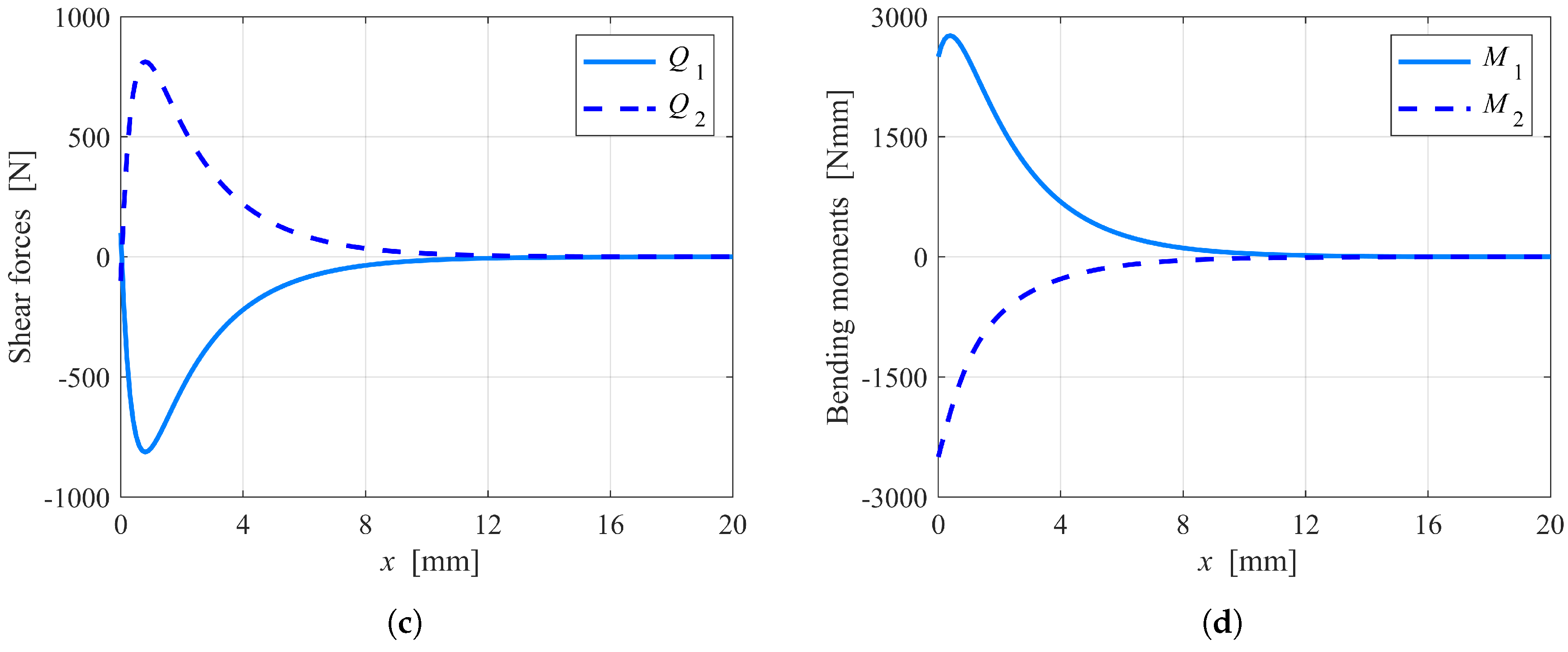
Figure 5 and Figure 6 show the plots of the interfacial stresses and internal forces as functions of the x-coordinate in the neighborhood of the crack tip for the UD//CP and UD//MD specimens, respectively. Both specimens were asymmetric with unbalance parameter ${\beta }_0\ne 0$. Hence, the analytical solution for the unbalanced case applied (see Section 3.3). For the DCB test, the specimen response corresponded to I/II mixed-mode fracture conditions: actually, both Figure 5a and Figure 6a show non-zero normal and shear stresses, which attained peak values at the crack tip cross-section. All of the internal forces started from the assigned values at the crack tip cross-section and then approached zero asymptotically.

Table 5. Energy release rate and mode mixity.

Specimen	${\mathcal{G}}_{\mathbf{I}}$	${\mathcal{G}}_{\mathbf{II}}$	$\mathcal{G}$	$\mathit{\psi }$
	(J/m2)	(J/m2)	(J/m2)	(deg)
UD//UD	339.7	0	339.7	0
UD//CP	403.4	11.4	414.8	−9.5
UD//MD	524.2	135.9	660.1	−27.0

reports the Mode I and II contributions to the energy release rate computed for the three analyzed specimens, along with the total energy release rate and mode-mixity angle. It is apparent that the relative amount of the Mode II contribution increased with the specimen asymmetry.

5.2. Effects of Interface Stiffness

Figure 7 shows a schematic of the double cantilever beam specimen loaded by uneven bending moments (DCB-UBM) test [63]. Here, this particular test configuration was used to illustrate the effects of interface stiffness, i.e., of the values of the interface elastic constants, $k_x$ and $k_z$, on the solution according to the proposed model.

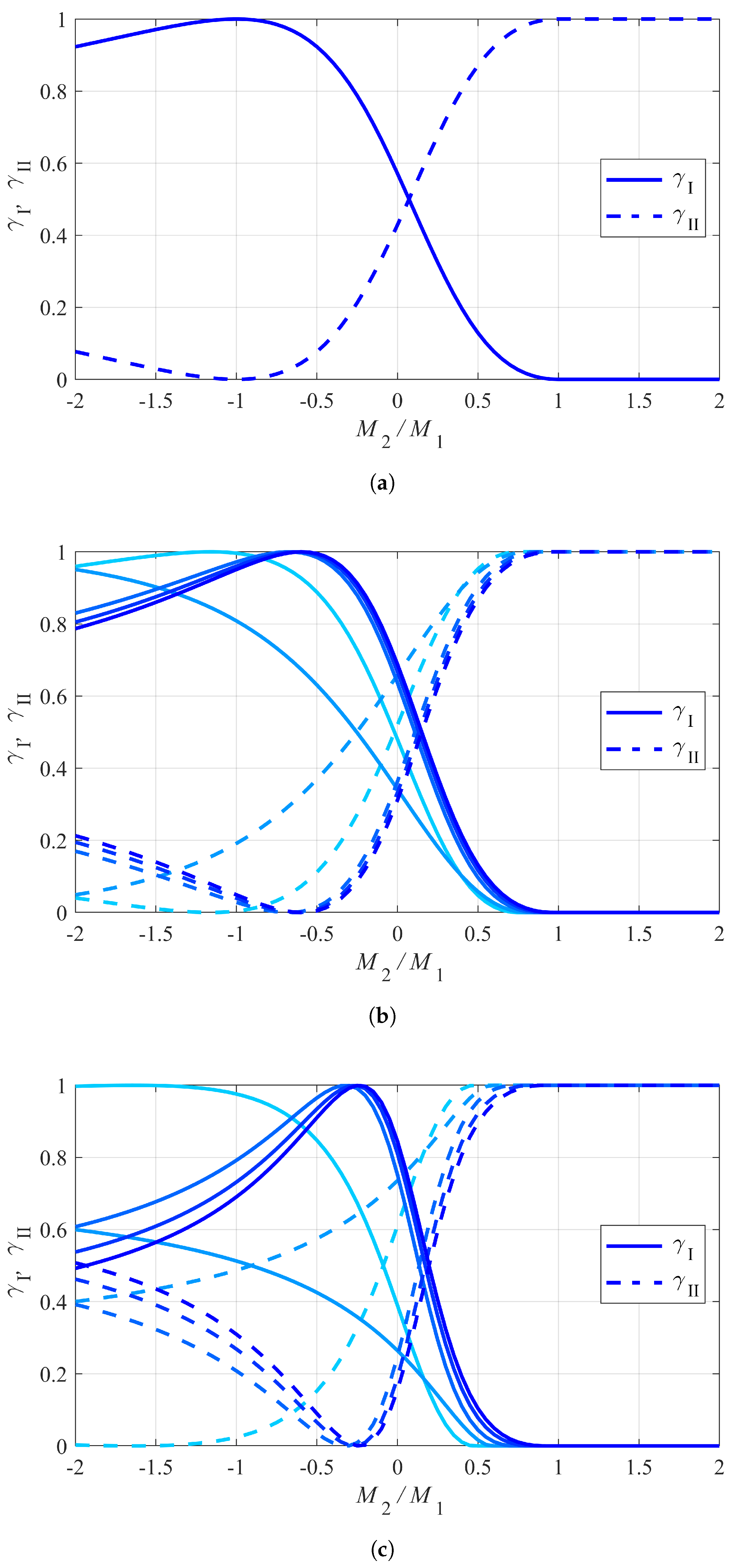
The same laminated specimens considered in the examples of Section 5.1 were again analyzed, but subjected to different loading conditions. The upper sublaminate was loaded by a unit bending couple, $M_1=1$ N m, while the lower sublaminate was loaded by a variable bending couple, $M_2$. Figure 8 shows the dimensionless Mode I and Mode II contributions to the energy release rate, ${\gamma }_{\mathrm{I}}={\mathcal{G}}_{\mathrm{I}}/\mathcal{G}$ and ${\gamma }_{\mathrm{II}}={\mathcal{G}}_{\mathrm{II}}/\mathcal{G}$, as functions of the bending moment ratio, $M_2/M_1$.

For the UD//UD specimen (Figure 8a), the modal contributions to $\mathcal{G}$ turned out to be independent of the interface stiffness. This result was due to the mid-plane symmetry of the specimen and the independence of the crack tip bending moments on the delamination length. In this case, also the mode mixity depended uniquely on the bending moment ratio, $M_2/M_1$. In particular, it can be noted how pure Mode I fracture conditions (${\gamma }_{\mathrm{II}}=0$) were obtained for $M_2=-M_1$, while pure Mode II fracture conditions (${\gamma }_{\mathrm{I}}=0$) were obtained for $M_2=M_1$. Values of $M_2/M_1$ greater than one also corresponded to pure Mode II because of the incompressibility constraint introduced for ${\mathcal{G}}_{\mathrm{I}}$ in Equation (44).

Instead, for both the UD//CP (Figure 8b) and UD//MD specimens (Figure 8c), the modal contributions to $\mathcal{G}$ depended on the values of the interface elastic constants, $k_x$ and $k_z$. For each modal contribution, the plots show five curves with different shades of blue: from lighter to darker, and these correspond to $k_x=k_z={10}^2,{10}^3,{10}^4,\mathrm{and}{10}^5{\mathrm{N}/\mathrm{mm}}^3$; the darkest curves represent the limit case $k_x=k_z\to +\infty$, which corresponds to a rigid interface model [51]. For the specimens considered, also the mode mixity and the conditions for pure fracture modes depended on the interface stiffness.

The range of values adopted for $k_x$ and $k_z$ in the previous plots may look quite wide. Indeed, this range corresponds to real values that may be obtained when performing a compliance calibration with experimental results or numerical simulations [62]. The results obtained suggest that the elastic interface model is potentially capable of highly-accurate prediction and interpretation of experimental results, provided that the appropriate values of the interface elastic constants are selected. To this aim, it would be useful to validate the theoretical predictions obtained with experimental results, such as those obtained by Davidson et al. [64,65]. Such a comparison, similar to the one carried out by Harvey et al. to validate different mixed-mode partition theories [66,67], will be the subject of future work.

6. Conclusions

An elastic interface model was introduced for the analysis of delamination in bending-extension coupled laminated beams with through-the-width delamination cracks. The analytical solution obtained applies to a wide class of multi-directional fiber-reinforced composite laminates, including cross-ply laminates, provided that their stacking sequences allow them to be modeled as plane beams. Examples illustrated the application of the model to the analysis of the double cantilever beam test in I/II mixed-mode fracture conditions. Furthermore, the effects of the interface stiffness on the model predictions were discussed with reference to the DCB specimen loaded with uneven bending moments.

By suitably adapting the boundary conditions, the outlined solution can be easily used to analyze different delamination toughness test configurations, as well as delamination behavior in real structural elements and debonding of adhesively-bonded joints.

The proposed model is potentially capable of highly-accurate prediction and interpretation of experimental results, provided that the appropriate interface stiffness is defined. In this respect, it will be useful to compare the model predictions with the results of experimental tests available in the literature. Future developments also include the extension of the model to fully-coupled laminates, for which plate theory must be used, and I/II/III mixed-mode fracture conditions are expected.

References

- Talreja, R.; Singh, C.V. Damage and Failure of Composite Materials; Cambridge University Press: Cambridge, UK, 2012; ISBN 978-0-521-81942-8. [Google Scholar]
- Garg, A.C. Delamination—A damage mode in composite structures. Eng. Fract. Mech. 1988, 29, 557–584. [Google Scholar] [CrossRef]
- Bolotin, V.V. Delaminations in composite structures: its origin, buckling, growth and stability. Compos. Part B Eng. 1996, 27, 129–145. [Google Scholar] [CrossRef]
- Tay, T.E. Characterization and analysis of delamination fracture in composites: An overview of developments from 1990 to 2001. Appl. Mech. Rev. 2003, 56, 1–31. [Google Scholar] [CrossRef]
- Senthil, K.; Arockiarajan, A.; Palaninathan, R.; Santhosh, B.; Usha, K.M. Defects in composite structures: Its effects and prediction methods—A comprehensive review. Compos. Struct. 2013, 106, 139–149. [Google Scholar] [CrossRef]
- Tabiei, A.; Zhang, W. Composite Laminate Delamination Simulation and Experiment: A Review of Recent Development. Appl. Mech. Rev. 2018, 70, 030801. [Google Scholar] [CrossRef]
- Bucur, V. (Ed.) Delamination in Wood, Wood Products and Wood-Based Composites; Springer: Dordrecht, The Netherlands, 2011; ISBN 978-90-481-9549-7. [Google Scholar] [CrossRef]
- Minatto, F.D.; Milak, P.; De Noni, A.; Hotza, D.; Montedo, O.R.K. Multilayered ceramic composites—A review. Adv. Appl. Ceram. 2015, 114, 127–138. [Google Scholar] [CrossRef]
- Friedrich, K. (Ed.) Application of Fracture Mechanics to Composite Materials; Elsevier: Amsterdam, The Netherlands, 1989; ISBN 978-0-444-87286-9. [Google Scholar]
- Carlsson, L.A.; Adams, D.F.; Pipes, R.B. Experimental Characterization of Advanced Composite Materials, 4th ed.; CRC Press: Boca Raton, FL, USA, 2014; ISBN 978-1-4398-4858-6. [Google Scholar]
- Hutchinson, J.W.; Suo, Z. Mixed mode cracking in layered materials. Adv. Appl. Mech. 1991, 29, 63–191. [Google Scholar] [CrossRef]
- Kanninen, M.F. An augmented double cantilever beam model for studying crack propagation and arrest. Int. J. Fract. 1973, 9, 83–92. [Google Scholar] [CrossRef]
- Bruno, D.; Grimaldi, A. Delamination failure of layered composite plates loaded in compression. Int. J. Solids Struct. 1990, 26, 313–330. [Google Scholar] [CrossRef]
- Allix, O.; Ladevèze, P. Interlaminar interface modeling for the prediction of delamination. Compos. Struct. 1992, 22, 235–242. [Google Scholar] [CrossRef]
- Corigliano, A. Formulation, identification and use of interface models in the numerical analysis of composite delamination. Int. J. Solids Struct. 1993, 30, 2779–2811. [Google Scholar] [CrossRef]
- Allix, O.; Ladevèze, P.; Corigliano, A. Damage analysis of interlaminar fracture specimens. Compos. Struct. 1995, 31, 61–74. [Google Scholar] [CrossRef]
- Point, N.; Sacco, E. A delamination model for laminated composites. Int. J. Solids Struct. 1996, 33, 483–509. [Google Scholar] [CrossRef]
- Bruno, D.; Greco, F. Mixed mode delamination in plates: a refined approach. Int. J. Solids Struct. 2001, 38, 9149–9177. [Google Scholar] [CrossRef]
- Qiao, P.; Wang, J. Mechanics and fracture of crack tip deformable bi-material interface. Int. J. Solids Struct. 2004, 41, 7423–7444. [Google Scholar] [CrossRef]
- Szekrényes, A. Improved analysis of unidirectional composite delamination specimens. Mech. Mater. 2007, 39, 953–974. [Google Scholar] [CrossRef]
- Bennati, S.; Valvo, P.S. Delamination growth in composite plates under compressive fatigue loads. Compos. Sci. Technol. 2006, 66, 248–254. [Google Scholar] [CrossRef]
- Bennati, S.; Colleluori, M.; Corigliano, D.; Valvo, P.S. An enhanced beam-theory model of the asymmetric double cantilever beam (ADCB) test for composite laminates. Compos. Sci. Technol. 2009, 69, 1735–1745. [Google Scholar] [CrossRef]
- Bennati, S.; Fisicaro, P.; Valvo, P.S. An enhanced beam-theory model of the mixed-mode bending (MMB) test—Part I: Literature review and mechanical model. Meccanica 2013, 48, 443–462. [Google Scholar] [CrossRef]
- Bennati, S.; Fisicaro, P.; Valvo, P.S. An enhanced beam-theory model of the mixed-mode bending (MMB) test—Part II: Applications and results. Meccanica 2013, 48, 465–484. [Google Scholar] [CrossRef]
- Xie, J.; Waas, A.; Rassaian, M. Analytical predictions of delamination threshold load of laminated composite plates subject to flexural loading. Compos. Struct. 2017, 179, 181–194. [Google Scholar] [CrossRef]
- Dimitri, R.; Tornabene, F.; Zavarise, G. Analytical and numerical modeling of the mixed-mode delamination process for composite moment-loaded double cantilever beams. Compos. Struct. 2018, 187, 535–553. [Google Scholar] [CrossRef]
- Park, K.; Paulino, G.H. Cohesive Zone Models: A Critical Review of Traction-Separation Relationships Across Fracture Surfaces. Appl. Mech. Rev. 2013, 64, 060802. [Google Scholar] [CrossRef]
- Dimitri, R.; Trullo, M.; De Lorenzis, L.; Zavarise, G. Coupled cohesive zone models for mixed-mode fracture: A comparative study. Eng. Fract. Mech. 2015, 148, 145–179. [Google Scholar] [CrossRef]
- Borg, R.; Nilsson, L.; Simonsson, K. Simulation of delamination in fiber composites with a discrete cohesive failure model. Compos. Sci. Technol. 2001, 61, 667–677. [Google Scholar] [CrossRef]
- Camanho, P.P.; Dávila, C.G.; de Moura, M.F. Numerical simulation of mixed-mode progressive delamination in composite materials. J. Compos. Mater. 2003, 37, 1415–1438. [Google Scholar] [CrossRef]
- Yang, Q.; Cox, B. Cohesive models for damage evolution in laminated composites. Int. J. Fract. 2005, 133, 107–137. [Google Scholar] [CrossRef]
- Parmigiani, J.P.; Thouless, M.D. The effects of cohesive strength and toughness on mixed-mode delamination of beam-like geometries. Eng. Fract. Mech. 2007, 74, 2675–2699. [Google Scholar] [CrossRef] [Green Version]
- Turon, A.; Dávila, C.G.; Camanho, P.P.; Costa, J. An engineering solution for mesh size effects in the simulation of delamination using cohesive zone models. Eng. Fract. Mech. 2007, 74, 1665–1682. [Google Scholar] [CrossRef]
- Harper, P.W.; Hallett, S.R. Cohesive zone length in numerical simulations of composite delamination. Eng. Fract. Mech. 2008, 75, 4774–4792. [Google Scholar] [CrossRef] [Green Version]
- Sørensen, B.F.; Jacobsen, T.K. Characterizing delamination of fiber composites by mixed mode cohesive laws. Compos. Sci. Technol. 2009, 69, 445–456. [Google Scholar] [CrossRef]
- Xie, J.; Waas, A.; Rassaian, M. Closed-form solutions for cohesive zone modeling of delamination toughness tests. Int. J. Solids Struct. 2016, 88–89, 379–400. [Google Scholar] [CrossRef]
- Wu, C.; Gowrishankar, S.; Huang, R.; Liechti, K.M. On determining mixed-mode traction–separation relations for interfaces. Int. J. Fract. 2016, 202, 1–19. [Google Scholar] [CrossRef]
- Wu, C.; Huang, R.; Liechti, K.M. Simultaneous extraction of tensile and shear interactions at interfaces. J. Mech. Phys. Solids 2019, 125, 225–254. [Google Scholar] [CrossRef]
- Da Silva, L.F.M.; das Neves, P.J.C.; Adams, R.D.; Spelt, J.K. Analytical models of adhesively bonded joints—Part I: Literature survey. Int. J. Adhes. Adhes. 2009, 29, 319–330. [Google Scholar] [CrossRef]
- Bigwood, D.A.; Crocombe, A.D. Elastic analysis and engineering design formulae for bonded joints. Int. J. Adhes. Adhes. 1989, 9, 229–242. [Google Scholar] [CrossRef]
- Krenk, S. Energy release rate of symmetric adhesive joints. Eng. Fract. Mech. 1992, 43, 549–559. [Google Scholar] [CrossRef]
- Penado, F.E. A closed form solution for the energy release rate of the double cantilever beam specimen with an adhesive layer. J. Compos. Mater. 1993, 27, 383–407. [Google Scholar] [CrossRef]
- Bennati, S.; Taglialegne, L.; Valvo, P.S. Modelling of interfacial fracture of layered structures. In Proceedings of the ECF 18—18th European Conference on Fracture, Dresden, Germany, 30 August–3 September 2010; ISBN 978-3-00-031802-3. [Google Scholar]
- Liu, Z.; Huang, Y.; Yin, Z.; Bennati, S.; Valvo, P.S. A general solution for the two-dimensional stress analysis of balanced and unbalanced adhesively bonded joints. Int. J. Adhes. Adhes. 2014, 54, 112–123. [Google Scholar] [CrossRef] [Green Version]
- Jiang, W.; Qiao, P. An improved four-parameter model with consideration of Poisson’s effect on stress analysis of adhesive joints. Eng. Struct. 2015, 88, 203–215. [Google Scholar] [CrossRef]
- Zhang, Z.W.; Li, Y.S.; Liu, R. An analytical model of stresses in adhesive bonded interface between steel and bamboo plywood. Int. J. Solids Struct. 2015, 52, 103–113. [Google Scholar] [CrossRef]
- Blackman, B.R.K.; Hadavinia, H.; Kinloch, A.J.; Williams, J.G. The use of a cohesive zone model to study the fracture of fiber composites and adhesively-bonded joints. Int. J. Fract. 2003, 119, 25–46. [Google Scholar] [CrossRef]
- Li, S.; Thouless, M.D.; Waas, A.M.; Schroeder, J.A.; Zavattieri, P.D. Mixed-mode cohesive-zone models for fracture of an adhesively bonded polymer—Matrix composite. Eng. Fract. Mech. 2006, 73, 64–78. [Google Scholar] [CrossRef]
- Jones, R.M. Mechanics of Composite Materials, 2nd ed.; Taylor & Francis Inc.: Philadelphia, PA, USA, 1999; ISBN 978-1560327127. [Google Scholar]
- Schapery, R.A.; Davidson, B.D. Prediction of energy release rate for mixed-mode delamination using classical plate theory. Appl. Mech. Rev. 1990, 43, S281–S287. [Google Scholar] [CrossRef]
- Valvo, P.S. On the calculation of energy release rate and mode mixity in delaminated laminated beams. Eng. Fract. Mech. 2016, 165, 114–139. [Google Scholar] [CrossRef]
- Tsokanas, P.; Loutas, T. Hygrothermal effect on the strain energy release rates and mode mixity of asymmetric delaminations in generally layered beams. Eng. Fract. Mech. 2019, 214, 390–409. [Google Scholar] [CrossRef]
- Taglialegne, L. Modellazione Meccanica Della Frattura Interlaminare di Provini in Composito Non Simmetrici. Master’s Thesis, University of Pisa, Pisa, Italy, 2014. Available online: http://etd.adm.unipi.it/theses/available/etd-09172014-092832 (accessed on 23 July 2019).
- Davidson, B.D.; Hu, H.; Schapery, R.A. An Analytical Crack-Tip Element for Layered Elastic Structures. J. Appl. Mech. 1995, 62, 294–305. [Google Scholar] [CrossRef]
- Wang, J.; Qiao, P. Interface crack between two shear deformable elastic layers. J. Mech. Phys. Solids 2004, 52, 891–905. [Google Scholar] [CrossRef]
- Timoshenko, S.P. Strength of Materials, Vol. 1: Elementary Theory And Problems, 3rd ed.; D. Van Nostrand: New York, NY, USA, 1955; ISBN 978-0442085414. [Google Scholar]
- Rice, J.R. A path independent integral and the approximate analysis of strain concentrations by notches and cracks. J. Appl. Mech. 1968, 35, 379–386. [Google Scholar] [CrossRef]
- Arouche, M.M.; Wang, W.; Teixeira de Freitas, S.; de Barros, S. Strain-based methodology for mixed-Mode I+II fracture: A new partitioning method for bi-material adhesively bonded joints. J. Adhes. 2019, 95, 385–404. [Google Scholar] [CrossRef]
- Vannucci, P.; Verchery, G. A special class of uncoupled and quasi-homogeneous laminates. Compos. Sci. Technol. 2001, 61, 1465–1473. [Google Scholar] [CrossRef]
- Garulli, T.; Catapano, A.; Fanteria, D.; Jumel, J.; Martin, E. Design and finite element assessment of fully uncoupled multi-directional layups for delamination tests. J. Compos. Mater. 2019. [Google Scholar] [CrossRef]
- Samborski, S. Numerical analysis of the DCB test configuration applicability to mechanically coupled Fiber Reinforced Laminated Composite beams. Compos. Struct. 2016, 152, 477–487. [Google Scholar] [CrossRef]
- Bennati, S.; Valvo, P.S. An experimental compliance calibration strategy for mixed-mode bending tests. Proc. Mater. Sci. 2014, 3, 1988–1993. [Google Scholar] [CrossRef]
- Sørensen, B.F.; Jørgensen, K.; Jacobsen, T.K.; Østergaard, R.C. DCB-specimen loaded with uneven bending moments. Int. J. Fract. 2006, 141, 163–176. [Google Scholar] [CrossRef]
- Davidson, B.D.; Gharibian, S.J.; Yu, L. Evaluation of energy release rate-based approaches for predicting delamination growth in laminated composites. Int. J. Fract. 2000, 105, 343–365. [Google Scholar] [CrossRef]
- Davidson, B.D.; Bialaszewski, R.D.; Sainath, S.S. A non-classical, energy release rate based approach for predicting delamination growth in graphite reinforced laminated polymeric composites. Compos. Sci. Technol. 2006, 66, 1479–1496. [Google Scholar] [CrossRef]
- Harvey, C.M.; Wang, S. Experimental assessment of mixed-mode partition theories. Compos. Struct. 2012, 94, 2057–2067. [Google Scholar] [CrossRef]
- Harvey, C.M.; Eplett, M.R.; Wang, S. Experimental assessment of mixed-mode partition theories for generally laminated composite beams. Compos. Struct. 2015, 124, 10–18. [Google Scholar] [CrossRef] [Green Version]
- Bednarcyk, B.A.; Aboudi, J.; Yarrington, P.W.; Collier, C.S. Simplified Shear Solution for Determination of the Shear Stress Distribution in a Composite Panel From the Applied Shear Resultant. In Proceedings of the 49th AIAA/ASME/ASCE/AHS/ASC Structures, Structural Dynamics, and Materials Conference, Schaumburg, IL, USA, 7–10 April 2008. [Google Scholar] [CrossRef]
- Kumar, R.; Nath, J.K.; Pradhan, M.K.; Kumar, R. Analysis of Laminated Composite Using Matlab. In Proceedings of the ICMEET 2014—1st International Conference on Mechanical Engineering: Emerging Trends for Sustainability, MANIT, Bhopal, India, 29–31 January 2014. [Google Scholar]
- Wallner-Novak, M.; Augustin, M.; Koppelhuber, J.; Pock, K. Cross-Laminated Timber Structural Design; proHolz: Vienna, Austria, 2018; Volume II, ISBN 978-3-902320-96-4. [Google Scholar]
Figure 1.
Laminated beam with through-the-width delamination.
Figure 2.
Crack-tip element: (a) definition; (b) model.
Figure 3.
Double cantilever beam test.
Figure 4.
UD//UD specimen: (a) interfacial stresses, (b) axial forces, (c) shear forces, and (d) bending moments in the crack tip neighborhood.
Figure 5.
UD//CP specimen: (a) interfacial stresses, (b) axial forces, (c) shear forces, and (d) bending moments in the crack tip neighborhood.
Figure 6.
UD//MD specimen: (a) interfacial stresses, (b) axial forces, (c) shear forces, and (d) bending moments in the crack tip neighborhood.
Figure 7.
Double cantilever beam specimen with uneven bending moments.
Figure 8.
Dimensionless modal contributions to energy release rate vs. sublaminate bending moment ratio: (a) UD//UD specimen, (b) UD//CP specimen, and (c) UD//MD specimen.