Exploiting Deep Learning for Wind Power Forecasting Based on Big Data Analytics

Abstract

Recently, power systems are facing the challenges of growing power demand, depleting fossil fuel and aggravating environmental pollution (caused by carbon emission from fossil fuel based power generation). The incorporation of alternative low carbon energy generation, i.e., Renewable Energy Sources (RESs), becomes crucial for energy systems. Effective Demand Side Management (DSM) and RES incorporation enable power systems to maintain demand, supply balance and optimize energy in an environmentally friendly manner. The wind power is a popular energy source because of its environmental and economical benefits. However, the uncertainty of wind power makes its incorporation in energy systems really difficult. To mitigate the risk of demand-supply imbalance, an accurate estimation of wind power is essential. Recognizing this challenging task, an efficient deep learning based prediction model is proposed for wind power forecasting. The proposed model has two stages. In the first stage, Wavelet Packet Transform (WPT) is used to decompose the past wind power signals. Other than decomposed signals and lagged wind power, multiple exogenous inputs (such as, calendar variable and Numerical Weather Prediction (NWP)) are also used as input to forecast wind power. In the second stage, a new prediction model, Efficient Deep Convolution Neural Network (EDCNN), is employed to forecast wind power. A DSM scheme is formulated based on forecasted wind power, day-ahead demand and price. The proposed forecasting model’s performance was evaluated on big data of Maine wind farm ISO NE, USA.

1. Introduction

Due to the industrial revolution, power demand has increased and fossil fuels are used extensively, resulting in an alarming energy crisis [1]. To mitigate the energy crisis, regulative acts that encourage the utilization of renewable energy are promoted worldwide. Wind power has attracted a lot of attention as a Renewable Energy Sources (RES) recently. Wind power has gained popularity due to its characteristics of wide availability, low investment cost [2] and no carbon emission. Wind  power helps in reducing environmental pollution [3]. It is introduced worldwide as a way to reduce greenhouse gas emission. Moreover, replacing thermal generation with wind generation leads to a fuel cost saving as wind has zero fuel costs. According to the Global Wind Energy Council [4], the cumulative capacity of wind power reached 486 GW across the global market in 2016. Wind power is expected to significantly expand, leading to an overall zero emission power system [5,6]. The U.S. Department of Energy Target of Renewable Integration is responsible for providing 20% of the total energy through wind, by the year 2030 [7]. In this regard, the Independent System Operators (ISOs) are producing significant wind power and increasing their wind generation.

Wind power is majorly affected by meteorological conditions, especially wind speed. Wind power exhibits strongly volatile and intermittent behavior, resulting in uncertain power output. This uncertainty significantly affects the quality of power system operations, such as distribution, dispatching, peak load management [8], etc. The greatest challenge of adapting wind power on a large scale is the control of its uncertain output. The effective solution to this issue is the correct estimate of future wind power. The correct Wind Power Forecasting (WPF) helps in improving the operation scheduling of power systems. The operating schedule for backup generators and storage systems are optimized based on the accurate WPF. The accuracy of WPF determines the amount of cost curtailment for power generation [9]. A 1% improvement in WPF accuracy results in 0.06% reduction in generation system’s cost. An accurate WPF results in approximately $6 million cost saving in a large scale power system with 30% wind penetration level [10].

It is acknowledged widely that accurate WPF significantly reduces the risks of incorporating wind power in power supply systems [11]. Generally, the WPF results are in the deterministic form (i.e., point forecast). Reducing the forecasting errors of WPF is the focus of many researchers [12]. A point forecast is the estimated value of future wind energy. However, wind power is a random variable having a Probability Density Function (PDF), and point forecasts are unable to capture the uncertainty of this random variable. This is the limitation of the point forecasts. Therefore, point forecasts have limited use in stability and security analysis of power systems. To overcome the limitation of point forecasts, deep learning methods are widely used in the field of WPF. Deep Neural Networks (DNN) have the inherent property of automatic modeling of the wind power characteristics [13].

The energy data collected on high granularity proved to be a useful resource for wind power predictive analytics [14]. Recently, big data driven models show significant accuracy in wind power forecasting [15,16]. Deep Neural Networks (DNNs) model the big data with good accuracy [17,18].

Micro Grids (MGs) are Distributed Energy Sources (DERs). MGs are categorized into two categories: stand-alone and grid-connected MGs. MGs can either have RES generation (wind power, photovoltaic, hydro power, etc.) or fossil fuel based generation, or both. In this research work, a grid-connected MG is considered that has a Wind Power Plant (WPP). In the case of unequal demand and generation in MG, energy is traded with the Smart Grid (SG). Excessive wind power is sold to the SG in exchange for a subsidiary. To fulfill demand greater than wind generation, required energy is purchased from SG. To fulfill the growing energy demand in an economical way, Demand Side Management (DSM) strategies are developed. There are six methods of DSM: (i) peak clipping; (ii) valley filling; (iii) energy conversation; (iv) flexible load shape; (v) strategic load growth (load building); and (vi) load shifting. To adjust the controllable loads, an advanced DSM strategy is developed for the studied scenario.

The rest of the article is organized as follows. The related work is presented in Section 2. The enhanced model is discussed in Section 4. The system description and problem formulation are presented in Section 5 and Section 6, respectively. The results are analyzed in Section 7. Section 8 concludes this article. The proposed system model that forecasts wind power and performs DSM is shown in Figure 1. The methods used in the proposed model are illustrated by Figures 2 and 3 and results are shown in Figures 4–6. This work is an extension of the work in [19]. A WPF model was proposed in [19] and that research work includes Section 4, Section 7.2 and Section 7.3 and Figures 2 and 4.

2. Related Work

In this section, the literature on wind power forecasting [1,9,20,21,22,23,24,25,26,27,28,29,30,31,32,33,34,35,36,37], DSM [38,39,40] and electricity load and price forecasting [41,42] is reviewed. The brief salient features of related literature are presented in

Table 1. Overview of related work.

Inputs	Dataset	Algorithms
Past wind power	Delaware wind farm data, American National Renewable Energy Laboratory, 2006	Nelder–Mead simplex optimization algorithm, Bidirectional backward Extreme learning machine [1]
Wind power, IEEE 118-bus system parameters	Wind Integration National Dataset , National Renewable Energy Laboratory, CASIO, MISO, ISO NE, 2007–2013	PLEXOS tool, Flexible Energy Scheduling Tool for Integrating Variable generation tool [9]
Past hourly wind power	66 wind power plants data, Supervisory Control And Data Acquisition (SCADA)	Vector autoregression model, Least absolute shrinkage and selection operator [24]
Past wind power	Wind farm, Donegal, North West Ireland, June–July 2004	Temporally local Gaussian process [25]
10-min resolution: wind speed, wind power	Global Energy Forecasting Competition (GEFCom) 2014	Multi-model combination method: Sparse Bayesian learning, Kernel density estimation and Beta distribution fitting method [26]
5-minute resolution: wind speed, wind power	Wind power data, Australian Energy Market Operator (AEMO), 2005	Spatial empirical decomposition, Random Forest, Gradient boosting, Support vector machine [27]
Wind power, wind speed	Wind farm data, Ireland and USA, August 2006, October 2008	Hybrid deterministic-probabilistic method with Gaussian process [28]
10-min resolution: wind speed, wind power	National Renewable Energy Laboratory, 2005–2006	Ensemble method: Wavelet transform, Partial least squares regression, ANN [29]
Wind speed, wind power	GEFCom 2012	ANN, Gaussian process [30]
Past hourly wind power, past weather forecast: wind speed, wind direction, temperature and humidity	Wind power generation, Alberta, Canada	Improved Clonal selection algorithm, Wavelet neural networks, Maximum correntropy criterion [31]
Wind turbine parameters, wind speed, wind power	10-min wind farm data, SCADA	K-means clustering, Bagging ANN [32]
Wind power, weather forecasts	5 Wind farms data, Europe	Mutual information, Deep auto-encoders, Deep belief network [33]
Wind speed, wind power	National Renewable Energy Laboratory (NREL), 2004	Infinite feature selection method, RNN [34]
Day of the year, hour, wind speed, wind direction, temperature, humidity, pressure, generators out of service	MADE wind farm, ITER, Tenerife Island, Spain, January 2014–April 2016	Multi-layer perceptron with ReLU, Long short-term memory, Nonlinear autoregressive network with exogenous inputs [35]
5-min intervals past wind power	SIWF wind farm, China, 2011–2013	Wavelet transform, Ensemble CNN [36]
Wind speed, wind direction, temperature, humidity, pressure	MADE wind farm, ITER, Tenerife Island, Spain	Feed Forward ANN, SELU CNN, RNN [37]
Past consumption, solar radiation	Victorian solar dataset	Game theory model [38] *
Historic price and load	Hourly load and price data, NYISO, PJM, AEMO, 2010, 2013, 2014	Flexible wavelet packet transform, Nonlinear least square support vector machine, ARIMA, TV-ABC [39] *
Historic consumption, wind power, photovoltaic power	Micro grid data, Renewable Energy Laboratory, UPNa, 2014	Simple moving average, Central moving average [40] *

* Demand Side Management papers.

.

The wind power has a chaotic nature. Therefore, the incorporation of wind power in power supply systems is a risky task. To mitigate this risk, wind power forecasting is the most popular method. The wind power is forecasted using classical, statistical, data mining [9,20,21,22,23,24,25,26,27,28] and artificial intelligence methods [1,29,30,31,32,33,34]. The accuracy of wind power forecasting is important to avoid demand–supply imbalance. Therefore, researchers are still competing to improve the wind power forecasting accuracy.

In the literature, there are two types of wind power forecasting techniques:

(1) Time series (univariate): Past generation data are used to predict future generation [12,24,25,36]. Univariate data are decomposed to make it multidimensional. Generally, data are decomposed by Discrete Wavelet Transform (DWT), Empirical Mode Decomposition (EMD) or Wavelet Packet Transform (WPT).

(2) Multivariate: Multiple exogenous inputs, such as Numerical Weather Predictions (NWP) (wind speed, wind direction, temperature, humidity, pressure, etc.), hour, day of the year, etc. are used to predict wind power generation [1,9,26,27,28,29,30,31,32,33,34,37].

The Artificial Neural Networks (ANNs) have widely used for modeling the highly fluctuating wind power data [1,29,30,31,32]. In [29], the authors forecasted wind power using ensemble ANN. The wind power time series is decomposed using DWT and related features are selected using conditional mutual information. Ensemble ANN is used for short-term wind power prediction. A Gaussian process based ensemble ANN is implemented in paper [30]. Five Gaussian processes and 52 sub-models of ANN are used to predict 48 h wind power. The authors of [1] proposed a bidirectional Extreme Learning Machine (ELM) for 6 h ahead WPF. Nelder–Mead simplex optimization algorithm is proposed for ELM’s learning. ANNs combined with optimization techniques show a reasonable forecasting accuracy. However, the ANNs have a few limitations, such as over-training, sensitivity to initial set parameters and instability. The aforementioned methods are shallow learners, therefore, unable to learn the deep underlying structures hidden in the wind power data. To overcome the problem of shallow learning, the deep learning methods are introduced. Deep Neural Networks (DNNs) can model abstract features hidden in the data. The deep learning models have achieved better accuracy in WPF as compared to the ANN forecasting models [33,34,35,36,37]. The popular DNN methods used for WPF are Deep Belief Networks (DBNs) [33], Recurrent Neural Networks (RNNs) [34], Long Short-term Memory (LSTM) [35] and Convolution Neural Networks (CNNs) [36,37].

In [33], ensemble DBNs are utilized as the wind power forecasting model. The wind power time series is decomposed by EMD and predicted by DBN. The building blocks of DBN are Restricted Boltzmann Machines (RBMs). Several RMBs are stacked together to construct a DBN. The DBN training process consists of two main steps: greedy layer-wise pre training and fine-tuning. By increasing the number of inputs, the DBN’s computational complexity increase. The authors of [34] combined the RNN and infinite feature selection technique to address the WPF problem. RNN has recurrence operation and maintains data in the memory cells. CNN is superior to the DBN and RNN due to its less training time and efficient feature mining. CNN is a state-of-the-art deep learning method. It is the CNN’s characteristic that it can extract the spatial features automatically. CNN is the most popular method for extracting features from the images and widely used in the field of computer vision. The efficient feature extraction capability of CNN motivates us to exploit it for wind power forecasting. CNN successfully extracts the spatiotemporal correlations in wind power data [36,37]. Wang et al. proposed an ensemble CNN model [36]. Wind power time series is decomposed by DWT. Short-term wind power is predicted using ensemble CNN. In ensemble CNN, multiple CNNs are used for prediction of a data point. Prediction is performed by taking (weighted) vote of multiple predictions made by all the CNNs. In [37], an enhanced CNN is proposed for WPF. A new activation function, Scaled Exponential Linear Unit (SELU), is proposed. NWP inputs are used for short-term wind power forecasting. The afore mentioned CNN based prediction models perform reasonably well. However, the effect of using both decomposed and exogenous inputs simultaneously on the accuracy of prediction model still needs to be investigated. According to our limited knowledge, both the decomposed data and NWP are not simultaneously used as input for predicting wind power.

Therefore, in this paper, a wind power prediction method is proposed which takes wavelet packet decomposed past wind power, NWP and lagged wind power data as input. The second objective of this research work is the optimal load profiling with the incorporation of wind generation. Previously, the optimal load profile is achieved by load forecasting [38], price-demand forecasting [39] or load and generation forecasting [40]. In this work, the wind generation is also considered, in addition to day-ahead demand and price. By optimal, it means the goal is to achieve a load profile that reduces the generation from dispatchable sources in an economical manner. In this work, a DSM algorithm is proposed on the basis of day-ahead demand, LMP and wind power forecasting. The wind power forecasting and day-ahead demand of MG are used to calculate the difference in the load demand and wind generation. The load is adjusted by shifting it to the low consumption time (valley filling). Thus, the peak periods’ load is clipped and the valley periods are filled. The day-ahead LMP is used to calculate the day-ahead consumption cost. In this way, the objectives of energy management and DSM are achieved.

3. Contributions

In this paper, we are concerned with the problems of predicting the wind power and demand side management with the incorporation of wind power, demand and price. The uniqueness and originality of this work is given below. The contributions of this research work are listed below:

• A novel big data-driven wind power prediction model is proposed that combines the strengths of both the univariate and multivariate wind power forecasting techniques by using decomposed and exogenous inputs for forecasting; consequently, the forecasting accuracy is significantly enhanced.
• The proposed model employs an existing method wavelet packet decomposition and an enhanced method Efficient DCNN (EDCNN) for feature extraction and forecasting, respectively.
• A DSM algorithm is also proposed. The proposed DSM algorithm takes into account the day-ahead demand, day-ahead price and wind power.
• The proposed DSM algorithm reduces the consumption cost and improves the load profile to almost a normal shape.

4. Proposed Model

The proposed model for forecasting wind power generation (as shown in Figure 1) and the proposed DSM algorithm are discussed in this section.

4.1. Data Preprocess

The features and targets (wind power) are normalized using min-max normalization. The inputs to the forecasting model are shown in

Table 2. Inputs to the forecast model.

Input	Description
Dew point temperature	Past NWP forecast
Dry bulb temperature	Past NWP forecast
Wind speed	Past NWP forecast
Lagged wind power 1	Wind power (t-24)
Lagged wind power 2	Wind power (t-25)
Decomposed wind power	Wavelet decomposed past wind power
Hour	Time of the day

. Three types of inputs are given to the forecasting model: (i) NWP, i.e., dew point temperature, dry bulb temperature, and wind speed; (ii) past lagged values of wind power; and (iii) wavelet packet decomposed wind power. The wavelet decomposition is described in the next section.

4.2. Feature Engineering

The historical wind power signal is decomposed using WPT. The WPT is a general form of the wavelet decomposition, which performs a better signal analysis. WPT was introduced in 1992 by Coifman and Wickerhauser [43]. Unlike DWT, the WPT waveforms or packets are interpreted by three different parameters: frequency, position and scale (similar to the DWT). For every orthogonal wavelet function, multiple wavelet packets are generated, having different bases (Figure 2). With  the help of these bases, the input signal can be encoded in such a way that the global energy of signal is preserved and the exact signal can be reconstructed effectively. Multiple expansions of an input signal can be achieved using WPT. The most suitable decomposition is selected by calculating the entropy (e.g., Shannon entropy). The minimal representation of the relevant data based on a cost function is calculated in WPT. The benefit of the WPT is its characteristic of analyzing signals in different temporal as well as spatial positions. For highly nonlinear and oscillating signal such as wind power DWT does not guarantee good results [44]. In WPT, both the approximation and detail coefficients are further decomposed into approximation and detail coefficients as the wavelet tree grows deeper. Wavelet packet decomposition operation can be expressed by Equations (1) and (2). For a signal a to be decomposed, two filters of size $2N$ are applied on a. The corresponding wavelets are $h\left(n\right)$ and $g\left(n\right)$.

$$W_{2n}\left(a\right)=\sqrt{2}\sum _{k=0}^{2N-1}h\left(k\right)W_n(2a-k)$$

(1)

$$W_{2n+1}\left(a\right)=\sqrt{2}\sum _{k=0}^{2N-1}g\left(k\right)W_n(2a-k)$$

(2)

where the scaling factor is $W_0\left(a\right)=\varphi \left(a\right)$ and the wavelet function is $W_1\left(a\right)=\psi \left(a\right)$.

The past wind power signal is decomposed into 36 signals and the best representation of the input signal is selected through Shannon entropy.

After decomposing the past wind signals, the engineered features along with NWP variables (dew point, dry bulb, and wind speed), lagged wind power (w-24 and w-25) and time are input to the proposed forecasting model. The proposed forecasting model is discussed in the next section.

4.3. Efficient DCNN

Modified CNN is widely used for forecasting [45]. An enhanced CNN for wind power forecasting is discussed below. The inputs are given to the EDCNN for predicting day-ahead hourly wind power (24 values). Firstly, the functionality of trivial CNN is discussed in this section. Secondly, the proposed method EDCNN is explained.

CNN is the computational model of human visual cortex’s functionality. CNN has an excellent capability of extracting deep underlying features of data. The CNN effectively identifies the spatially local correlations in data through convolution operation. In the convolution operation, a filter is applied to a block of spatially adjacent neurons (Figure 3) and the result is passed through an activation function. This output of convolution layer becomes the input to next layer’s neurons. Thus, the input to every neuron of a layer is the output of a convolved block of the previous layer. Unlike ANN, the CNN training is efficient due to the weight sharing scheme. Due to the weight sharing, the learning efficiency improves. CNN is composed of three altering layers: (i) convolution layer; (ii) sampling layer; and (iii) fully connected layer.

The convolution operation can be explained by Equation (3). Suppose X = [$x_1$, $x_2$ ,$x_3$, …, $x_n$] is the vector of training samples and C = [$c_1$, $c_2$, $c_3$, …, $c_n$] is the vector of corresponding targets. n is the number of training samples. CNN attempts to learn the optimal filter weights and biases that minimize the forecasting error. CNN can be defined as:

$$Y_i^m=f(w^m\otimes X_i^m+b^m)$$

(3)

where i = [1,2,…, n] and m = [1, 2, …, M]. m is the number of layer to be learned. The filter weights of the mth layer is denoted by $w^m$. $b^m$ represents the corresponding biases and ⊗ is the convolution operator. $f(·)$ is the nonlinear activation function. $Y_i^m$ is the feature map generated by sample $X_i$ at layer m.

In the proposed forecasting method EDCNN, there are eleven layers: three convolution layers, three max pooling layers, two batch normalization layers, three ReLU (Rectified Linear Unit) layers, one modified fully connected layer and one modified output layer (Enhanced Regression Output Layer (EROL)). The number of filters in all convolution layers is 9. The number of neurons in all the hidden layers is 200. The functionality of two layers is modified to improve the forecasting performance of EDCNN. According to the ANN literature, there is no standard way to choose an optimal activation function. A modified activation function is employed in a hidden layer. The proposed activation function is the ensemble of results of three activation functions: hyperbolic tangent, sigmoid and radial base function (Equations (4)–(6), respectively). The proposed activation function, Equation (7), takes the average of the results of the three used activation functions.

$$TH=\frac{e^{xw}-e^{-xw}}{e^{xw}+e^{-xw}}$$

(4)

$$\sigma =\frac{e^{x}w}{1+e^{x}w}$$

(5)

$$\varphi =\varphi \parallel xw-c\parallel$$

(6)

$$F(x,w)=\frac{(TH+\sigma +\varphi )}{3}$$

(7)

where $xw$ is the intermediate output of a network layer (weighted sum of input) on which activation is to be applied to achieve the final output. $\varphi$ is the radial base function. The proposed activation function takes the average of the three aforementioned functions to calculate the results of corresponding hidden layer.

In the proposed output layer EROL, a modified objective function is embedded. The objective is to minimize the absolute percentage error between the forecast values and actual targets. The objective can be expressed as Equation (8):

$$minLoss(w,X_i,c_i)=L(w,X_i,c_i)$$

(8)

where $L(w,X_i,c_i)$ is the forecasting error or loss from sample $X_i$. The loss function is expressed as Equation (9):

$$L(w,X_i,c_i)=\frac{1}{n}\sum _{i=1}^n\left|\frac{Y_i-c_i}{Y_i}\right|100$$

(9)

where $c_i$ is the desired or actual target. $Y_i$ is the output of the output layer of EDCNN and its value is calculated as $Y_i=F\left({\sum }_{i=1}^n{X}_i{w}_i\right)$.

After forecasting the wind power, it is used in the DSM algorithm. The day-ahead Locational Marginal Price (LMP), day-ahead demand and forecasted wind power are the inputs to the proposed DSM algorithm. The proposed DSM algorithm is applied to the data of a smart grid-connected micro grid. The system description is presented in the next section.

5. System Description

A micro grid with the wind power plant that is connected to a smart grid is studied in this article. For the MG’s load management, three parameters are utilized: (i) wind power forecast; (ii) day-ahead demand/load; and (iii) day-ahead LMP. The LMP is the price of energy purchased from the SG in the case of insufficient generation of wind power. In the wind power generation, there are the following possible  cases:

5.1. Case 1

The first and simplest case is when the generated wind power is equal to the load. There is no gap between the generation and demanded power. In this case, no energy is required to be purchased from the SG. MG is self-sufficient.

5.2. Case 2

The wind power generated in the MG is greater than the required power. In this case, the excessive power is transmitted to the SG.

$$P_G=W-L\to SG$$

(10)

where $P_G$ is the active power, W is the wind power, L is the load and the transmission process is denoted by the symbol →. In exchange for this energy, the SG will give MG a subsidiary on the future price of future 24 h energy  purchase.

5.3. Case 3

Another case is when there is either no or lesser wind power as compared to the demand. In this case, the MG has to purchase the required power from the SG. If there is a subsidiary on price from the past, the price is reduced, otherwise the actual price is paid for purchasing energy. Generally, a 10–15% concession on energy price is offered as a subsidiary. In this case, the proposed demand management algorithm is applied to achieve the objectives listed below:

-

Load factor maximization

-

Consumption cost minimization

6. Problem Formulation

The wind power is forecasted for 24 h. The first objective is to maximize load factor for maximum utilization the power resource (RES generation from wind power plant). The second objective is to minimize the consumption cost.

$$Obj1=maximizeLF$$

(11)

$$Obj2=minimizeC$$

(12)

where LF is the load factor (Equation (13)) and C (Equation (14)) is the total consumption cost.

$$LF=\frac{\widehat{L}}{\overline{L}}$$

(13)

$$C=\sum _{i=1}^n{L}_i\times P_i$$

(14)

where $\widehat{L}$ is the sum of total load, $\overline{L}$ is the average load, L is the load vector, P is the LMP vector and the unit of LMP is $\$/MWh$. n is the length of the load and LMP vectors.

There are a few constraints of the system. The first constraint is that the demanded load must be equal to the load after applying the DSM scheme. The second constraint is that, after applying the DSM, the consumption cost should be less than the initial cost. The third constraint is that load factor must increase. The following are the constraints (Equations (15)–(17)):

$$L=L_{new}$$

(15)

$$C\le C_{old}$$

(16)

$$L{F}_{new}>LF$$

(17)

where L is load before DSM and $L_{new}$ is load after applying DSM. $C_{old}$ is the consumption cost before DSM and C is cost after DSM. $L{F}_{new}$ is the load factor after DSM. The purpose of the proposed DSM scheme is to bring the consumption as close to the normal distribution curve as possible.

Let the input vectors contain 24 values: W = wind power forecast, L = day-ahead demand and P = day-ahead LMP. The other variables used in the algorithm are: C = consumption cost, S = subsidiary, DWD = demand-wind power difference, $P_{new}$ = new adjusted price, and $L_{new}$ = new normally distributed load after applying DSM scheme.

Manage_Demand(·) is the proposed function for managing demand in an economical manner. This function will distribute the load in a normal form by shaving the peak periods and filling the valley periods (Algorithm 1). The resultant load profile achieved by this method will follow the normal distribution, approximately.

Algorithm 1 Algorithm for Demand Side Management (DSM).
Require:Input: [W, L, P]
1: Output: C
2: if W = L then	▹ Wind power is sufficient to fulfill demand
3:    $P_{new}=0$	▹ Wind power is sufficient that has no cost
4:    $L_{new}=L$	▹ Load is equal to wind power, so load adjustment is not performed
5:    $C=P_{new}\times L_{new}$	▹ Calculating consumption cost
6: else if W > L then	▹ Wind power is greater than demand
7:    $W-L\to SG$	▹ Excessive wind power is transmitted to the SG
8:    S = 0.9	▹ 10 % reduction in price is subsidiary for next power purchase
9:    $P_{new}=0$	▹ Wind power is sufficient that has no cost
10:    $L_{new}=L$	▹ Load is lesser than wind power, so load adjustment is not performed
11:    $C=P_{new}\times L_{new}$	▹ Calculating the consumption cost
12: else if $W\ge 0ANDW<L$ then	▹ Wind power is not sufficient to fulfill the demand
13:    $DWD=L-W$	▹ Finding demand that have to be fulfilled by the SG
14:    $L_{new}=Manage\_Demand(DWD,L)$	▹ Managing demand to distribute it normally
15:    if S = 0.9 then	▹ If there is subsidiary on the price, the price will be adjusted
16:        $P_{new}=P\times S$	▹ 10% reduction on price by subsidiary
17:        $C=P_{new}\times L_{new}$	▹ Calculating consumption cost
18:    else
19:        $P_{new}=P$	▹ If there is no subsidiary on price, price remains same
20:        $C=P_{new}\times L_{new}$	▹ Calculating consumption cost
21:    end if
22: end if
23: Manage_Demand Function
24: Function $L_{new}=Manage\_Demand(DWD,L)$
25: $\mu =mean\left(DWD\right)$		▹ Average of demand to be fulfilled by the SG
26: $\sigma =std\left(DWD\right)$	▹ Standard deviation of demand to be fulfilled by the SG
27: $SD=sum\left(DWD\right)$	▹ Sum of demand to be fulfilled by the SG
28: if DWD < $\mu$ then	▹ Checking each value of demand vector if it is smaller than mean
29:    $L^{\prime }=L+\sigma$	▹ When value is smaller, add standard deviation to make it closer to mean
30: else if DWD > $\mu$ then	▹ Checking each value of demand vector if it is greater than mean
31:    $L^{\prime }=L-\sigma$	▹ When value is larger, subtract standard deviation to make it closer to mean
32: end if
33: $SL=sum\left(L^{\prime }\right)$	▹ Taking sum of all values of new adjusted load vector
34: d = SL – SD	▹ Taking the difference of demanding load and new adjusted load
35: ⊳	▹ Now the demanded load and new load are adjusted to be equal
36: if d > 0 then	▹ Difference greater than zero means the new adjusted load is more than the demanded load
37:    $\left[idxCount\right]=L>\mu$	▹ Count is the number of values greater than average and index are their index
38:    $L_{new}=L\left(indx\right)-\frac{d}{count}$	▹ Subtracting the difference from all the larger values
39: else if d < 0 then	▹ Difference smaller than zero means the new adjusted load is lesser than the demanded
40:            load
41:    $\left[indxCount\right]=L<\mu$	▹ Count is the number of values that are smaller than average load
42:    $L_{new}=L\left(indx\right)+\frac{d}{count}$	▹ Adding the difference in all the smaller values
43: end if
44: [index  $L_{sorted}$] = Sort($L_{new}$)	▹ Sort will sort the $L_{new}$ in ascending order and return index of the sorted array
45:                    $L_{sorted}$
46: For i = 1 to 6	▹ Shift the peak load to the lowest load
47: j = i-1,   sf = 5*i    a = length($L_{new}$)	▹ Defining shifting factor
48: if index(i) > 6 then	▹ Shift the load to the lowest load that is not late night
49:    shftFac = $\frac{L_{new}\left(index(a-j)\right)}{sf}$
50:    $L_{new}$(index(i)) = $L_{new}$(index(i)) - shftFac	▹ Subtracting the shifting factor from the highest load
51:    $L_{new}$(index(a-j)) = $L_{new}$(index(a-j)) + shftFac	▹ Adding the shifting factor to the lowest load
52: end if
53: End For
54: End Function

7. Results and Analysis

The proposed algorithms were implemented using MATLAB R2018a on a computer system with core i3 processor, 4 GB RAM and 500 GB hard disk.

7.1. Data Description

The three-year hourly data of wind power were taken from ISO New England’s wind farm located in Maine. The duration of data utilized in this research was from January 2015 to December 2017. The data are publicly available for researchers on the ISO New England’s website [46].

7.2. Wind Power Analysis

Wind power is a widely available RES, therefore it is one the most popular and emerging power generation sources. The predictive analytics were performed on wind power data of Maine wind farms, ISO New England. According to the annual report, Maine wind farms annually produce approximately 900 MW energy, which contributes almost 14% of the total electricity in Maine. The wind power is directly proportional to the wind speed. In Maine, USA, the wind speed is affected by seasonality. The wind power in autumn is higher compared to the other seasons. The reason behind this is the fastest winds in coastal area of Maine, where the wind turbines are installed.

7.3. EDCNN Performance Evaluation

EDCNN was compared with two models, namely typical CNN and SELU CNN [37], for wind power forecasting (Figure 4). For performance evaluation of wind power forecasting, three evaluation indicators were used: Mean Absolute Error (MAE), Normalized Root Mean Square Error (NRMSE) and Mean Absolute Percentage Error (MAPE) (

Table 3. MAPE and NRMSE of proposed and compared methods.

Method	Season	MAPE	NRMSE	MAE
	Spring	8.42	2.34	3.34
	Summer	8.23	2.27	3.24
CNN	Autumn	7.9	2.65	3.36
	Winter	8.1	2.71	2.89
	Spring	3.47	0.12	3.1
	Summer	3.62	0.13	3.3
SELU CNN	Autumn	3.45	0.12	3.4
	Winter	3.27	0.17	3.2
	Spring	2.67	0.092	2.4
	Summer	2.43	0.096	2.24
EDCNN	Autumn	2.56	0.085	2.67
	Winter	2.62	0.094	2.18

). MAPE, NRMSE, and MAE are widely used to evaluate the performance of wind power forecasting models [22,26,47,48]. All the results shown in Figure 4 and Table 3 were taken on one day (24 h) of every season, i.e., 1 January (winter), 1 April (spring), 1 July (summer) and 1 October (autumn).

7.4. Statistical Analysis of EDCNN

The aforementioned error indicator (Table 3) were utilized for accuracy comparison of forecasting models. However, the lesser error or higher accuracy of a model does not guarantee its superiority over other models. A model is better as compared to another model if the difference between their accuracies is statistically significant. Different statistical tests are used to validate the significance of models, such as error analysis [49], Friedman test [50], Diebold–Mariano (DM) test [51], etc. To validate the performance of the proposed forecasting model EDCNN, a well-known statistical test, DM, was used. Diebold and Mariano proposed the classical Diebold–Mariano statistical test in 1995 [51]. The DM test evaluates the significant difference between forecasting errors to two models. The null hypothesis $H_0$ states that the models have equal accuracy (when the value of $d_t^{F{M}^1,F{M}^2}$ in Equation (18) is equal to zero). The alternative hypothesis $H_1$ is that one model is significantly more accurate as compared to the other mode (if the value of $d_t^{F{M}^1,F{M}^2}$ in Equation (18) is greater than zero, Model 1 is better than Model 2).

A vector of values that are to be forecasted are $X=[X_1,X_2,\dots ,X_n]$. Two prediction models $FM$ predict these values, i.e., $F{M}^1$ and $F{M}^2$. The forecasting errors of these models are:

$${\epsilon }^{F{M}^1}=[{\epsilon }_1^{F{M}^1},{\epsilon }_2^{F{M}^1},\dots ,{\epsilon }_n^{F{M}^1}]$$

$${\epsilon }^{F{M}^2}=[{\epsilon }_1^{F{M}^2},{\epsilon }_2^{F{M}^2},\dots ,{\epsilon }_n^{F{M}^2}]$$

In this study, the error metric used for DM is MAE. A covariance loss function $L(·)$ and differential loss was calculated in DM as Equation (18) [52]:

$$d_t^{F{M}^1,F{M}^2}=L\left({\epsilon }_t^{F{M}^1}\right)-L\left({\epsilon }_t^{F{M}^2}\right)$$

(18)

DM is widely used for validation of wind power forecasting [53]. The results of the DM test with confidence level of 95% are shown in

Table 4. Diebold–Mariano test results at a 95% confidence level and 5% significance level of p-value.

	DM Score
Season	EDCNN Compared to SELU CNN	SELU CNN Compared to CNN	EDCNN Compared to CNN
Spring DM-MAE	1.4252	0.0842	1.4256
Spring p-value	0.0432	0.9242	0.1248
Summer DM-MAE	1.3262	0.1024	1.3692
Summer p-valve	0.0326	0.8624	0.2142
Autumn DM-MAE	1.2714	0.1762	1.6728
Autumn p-vale	0.0196	0.0242	0.9242
Winter DM-MAE	1.4632	1.1426	1.2464
Winter p-value	0.02762	0.9862	0.7642

. DM was applied to the forecasting results of EDCNN and two compared methods: CNN and SELU CNN [37]. Three comparisons were performed, i.e., EDCNN with CNN, EDCNN with SELU CNN and CNN with SELU CNN. The EDCNN was better than CNN and SELU CNN and SELU CNN was better than CNN. The DM and p-values are shown in Table 4).

The significance level of p-value is 5%. In the comparison of EDCNN and SELU CNN, the $d_t^{F{M}^1,F{M}^2}$ value is more than zero, which depicts that the EDCNN model is significantly better than SELU CNN and similarly EDCNN is better than CNN. According to the DM’s hypothesis $H_1$, if the DM value is greater than zero, the first model is significantly better than the second model. The results in Table 4 show that the forecasting accuracy of EDCNN is significantly better than SELU CNN and CNN. SELU CNN is significantly better than CNN.

7.5. Analysis of Proposed DSM Algorithm

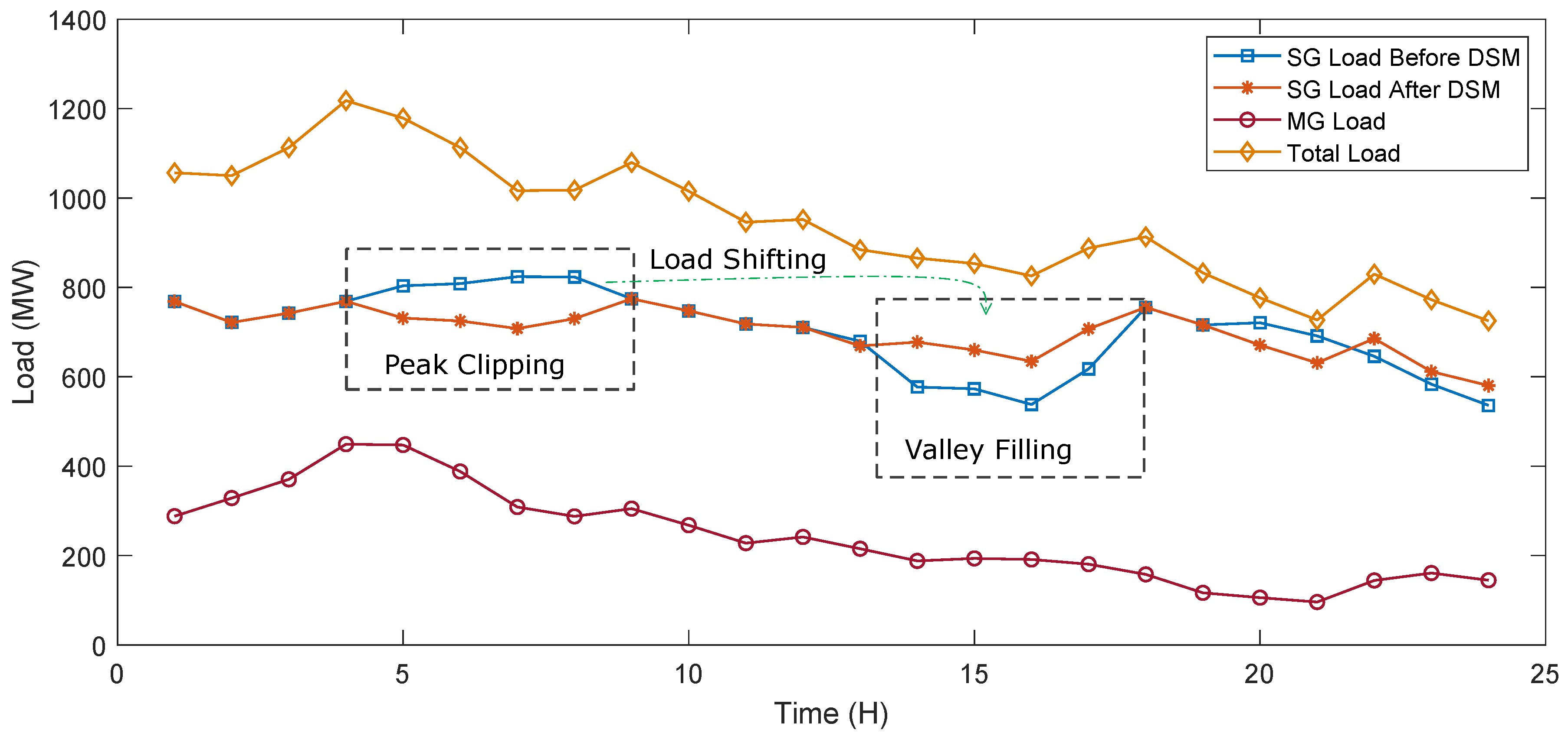
The results of the proposed DSM algorithm are shown in Figure 5. It is clearly seen that the load from peak hours are clipped and shifted to the off peak hours. The total power consumption, power supplied by the MG and power consumed from the SG are shown in Figure 5. The proposed DSM scheme was applied on the 24 h of 7 January 2017 because of the fairly reasonable wind power generation and no zero generation hour throughout the day that leads to a clear depiction of DSM results. The purpose of DSM is to reduce the consumption load of peak hours to minimize the usage of the dispatchable generators of SG. The MG only has WPP and no dispatchable generators. If the wind generation is insufficient, the MG purchase energy from SG. If energy demand of MG’s consumers is in the peak hours, then the load of MG is shifted from peak hours to off peak hours. An assumption is made that the MG encourages its consumers to shift their load from peak hours to off peak hours by offering some incentives and consumers shift their consumption load, which leads to overall load shifting in MG; consequently, the consumption cost of consumers is reduced. MG gets the advantage of not purchasing more energy from SG in peak hours (where price is higher than off peak hours’ price), which also leads to the purchasing cost reduction for MG. In this manner, the consumers will be satisfied and MG will have cost effective demand management.

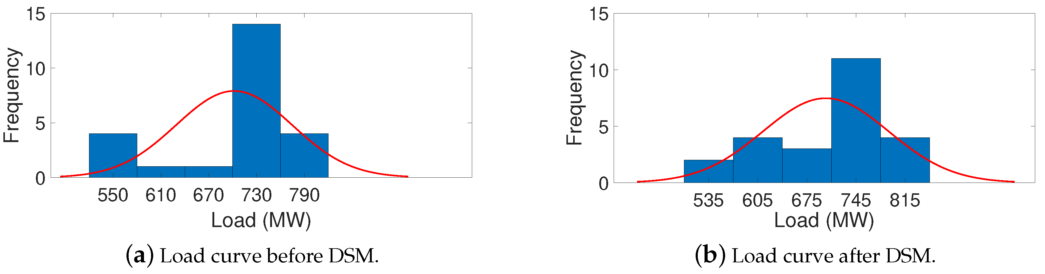
The proposed algorithm successfully shifts the load. In the proposed method, the load is shifted to off peak hours that are not late night. This is suitable because late night is sleeping hours, and the electricity cannot be consumed much. The goal of almost normally distributing the load profile is achieved. The load before DSM and after applying proposed DSM algorithm is shown in Figure 6. The load profile after DSM is more towards the normal distribution than the profile before DSM. The exact normal distribution of load cannot be achieved because of the fixed working hours. The electricity consumption in working hours cannot be shifted to other hours in a manner to achieve perfectly normal distribution of load. A portion of load is able to be shifted, which is known as shift-able load. The goal is to shift the shift-able load to improve load factor and reduce price that is achieved by applying proposed DSM.

Another goal of the proposed DSM algorithm is reducing the consumption cost. When the load is shifted to off peak hours, the consumption cost reduces due to the low power price in off peak hours. The reduction in consumption cost achieved by the proposed DSM algorithm is presented in

Table 5. Energy consumption cost reduction by the proposed DSM algorithm.

	Consumption Cost / Day ($)		Reduction / Day
Season	Before DSM	After DSM	Amount ($)	Percentage
Spring	483,330	475,170	8153$	1.7%
Summer	793,930.5	784,403	7527$	1.2%
Autumn	417,980.5	413,770.5	4210$	1%
Winter	3,347,106	3,305,006	42,109$	1.3%

, which shows the price before and after applying DSM algorithm. The cost reduced by DSM and its percentage is also mentioned. On average, 1.1% of total cost is reduced by applying the proposed DSM algorithm. When the proposed algorithm is applied to the 365 days of t 2017, approximately $2.25 million consumption cost is reduced. The DSM results of one day consumption cost from all four seasons are presented in Table 5. One day from every season of the year is taken for calculating results of DSM algorithm, i.e., 1 January (winter), 1 April (spring), 1 July (summer) and 1 October (autumn). The results confirm the effectiveness of proposed DSM algorithm as it achieves both the objectives: improving load factor and reducing consumption cost (as discussed in Section 6).

8. Conclusions and Future Work

This paper proposes a wind power forecasting scheme and a demand management strategy. To take part in the daily market that regulates the supply and demand in the Maine micro grid, a new demand management scheme is proposed that makes use of big data-driven wind power forecasting. The effective demand management is subject to the forecasting accuracy. A deep-learning technique EDCNN is developed to accurately predict the day-ahead hourly wind power on the Maine wind farm data. The numeric results validate the efficiency of the proposed model for wind power forecasting. The proposed DSM algorithm normally distributes the load. The results prove that the proposed DSM method successfully distribute the load, making load profile almost normally distributed. Moreover, the proposed DSM algorithm effectively reduces the consumption cost.

In the future work, shorter forecasting times will be considered, e.g., 12 h ahead. The day will be divided into daytime and nighttime to determine the impact of current conditions on wind power forecasting.

The connection possibilities of the power grid under the operating conditions of several wind farms will be analyzed by considering the throughput of power lines, permissible voltage values in the nodes and the power balance in the area.

The power grid in the area will be mapped by modeling the power lines, transformers, sources and loads to determine the impact of wind farm capacity maximization on the operation of the power system’s balance and stability.

The impact of wind power forecasting on the changes in power losses in the grid will also be determined in the future work.

References

- Zhao, Y.N.; Ye, L.; Li, Z.; Song, X.R.; Lang, Y.S.; Su, J. A novel bidirectional mechanism based on time series model for wind power forecasting. Appl. Energy 2016, 177, 793–803. [Google Scholar] [CrossRef]
- U.S. Department of Energy. Staff Report to the Secretary on Electricity Markets and Reliability. 2017. Available online: https://www.energy.gov/downloads/download-staff-report-secretary-electricity-markets-and-reliability (accessed on 8 June 2019).
- Jong, P.; Kiperstok, A.; Sanchez, A.S.; Dargaville, R.; Torres, E.A. Integrating large scale wind power into the electricity grid in the Northeast of Brazil. Energy 2016, 100, 401–415. [Google Scholar] [CrossRef]
- Global Wind Energy Council. GWEC Global Wind Report 2016. Available online: https://gwec.net/publications/global-wind-report-2/global-wind-report-2016 (accessed on 8 June 2019).
- Shafiee, M.; Brennan, F.; Espinosa, I.A. A parametric whole life cost model for offshore wind farms. Int. J. Life Cycle Assess. 2016, 21, 961–975. [Google Scholar] [CrossRef] [Green Version]
- Tomporowski, A.; Flizikowski, J.; Kasner, R.; Kruszelnicka, W. Environmental control of wind power technology. Rocznik Ochrona Srodowiska 2017, 19, 694–714. [Google Scholar]
- U.S. Department of Energy, 20% Wind Energy by 2030: Increasing Wind Energy’s Contribution to US Electricity Supply, Energy Efficiency and Renewable Energy (EERE). 2008. Available online: https://www.energy.gov/eere/wind (accessed on 8 June 2019).
- Athari, M.H.; Wang, Z. Impacts of Wind Power Uncertainty on Grid Vulnerability to Cascading Overload Failures. IEEE Trans. Sustain. Energy 2018, 9, 128–137. [Google Scholar] [CrossRef]
- Wang, Q.; Martinez-Anido, C.B.; Wu, H.; Florita, A.R.; Hodge, B.M. Quantifying the economic and grid reliability impacts of improved wind power forecasting. IEEE Trans. Sustain. Energy 2016, 7, 1525–1537. [Google Scholar] [CrossRef]
- Swinand, G.P.; Mahoney, A.O. Estimating the impact of wind generation and wind forecast errors on energy prices and costs in Ireland. Renew. Energy 2015, 75, 468–473. [Google Scholar] [CrossRef] [Green Version]
- Chen, Z. Wind power in modern power systems. J. Mod. Power Syst. Clean Energy 2013, 1, 2–13. [Google Scholar] [CrossRef] [Green Version]
- Haque, A.U.; Nehrir, M.H.; Mandal, P. A hybrid intelligent model for deterministic and quantile regression approach for probabilistic wind power forecasting. IEEE Trans. Power Syst. 2014, 29, 1663–1672. [Google Scholar] [CrossRef]
- Juban, J.; Siebert, N.; Kariniotakis, G.N. Probabilistic short-term wind power forecasting for the optimal management of wind generation. In Proceedings of the 2007 IEEE Lausanne Power Tech, Lausanne, Switzerland, 1–5 July 2007; pp. 683–688. [Google Scholar]
- Zhou, K.; Fu, C.; Yang, S. Big data driven smart energy management: From big data to big insights. Renew. Sustain. Energy Rev. 2016, 56, 215–225. [Google Scholar] [CrossRef]
- Haupt, S.E.; Kosovic, B. Variable generation power forecasting as a big data problem. IEEE Trans. Sustain. Energy 2016, 8, 725–732. [Google Scholar] [CrossRef]
- Zhang, J.; Cui, M.; Hodge, B.M.; Florita, A.; Freedman, J. Ramp forecasting performance from improved short-term wind power forecasting over multiple spatial and temporal scales. Energy 2017, 122, 528–541. [Google Scholar] [CrossRef] [Green Version]
- Zhang, Q.; Yang, L.T.; Chen, Z.; Li, P. A survey on deep learning for big data. Inf. Fusion 2018, 42, 146–157. [Google Scholar] [CrossRef]
- Najafabadi, M.M.; Villanustre, F.; Khoshgoftaar, T.M.; Seliya, N.; Wald, R.; Muharemagic, E. Deep learning applications and challenges in big data analytics. J. Big Data 2015, 2, 1–15. [Google Scholar] [CrossRef]
- Mujeeb, S.; Javaid, N.; Gul, H.; Daood, N.; Shabbir, S.; Arif, A. Wind Power Forecasting Based on Efficient Deep Convolution Neural Networks. In Proceedings of the 3PGCIC Conference, Antwerp, Belgium, 7–9 November 2019. [Google Scholar]
- Xu, Q.; He, D.; Zhang, N.; Kang, C.; Xia, Q.; Bai, J.; Huang, J. A short-term wind power forecasting approach with adjustment of numerical weather prediction input by data mining. IEEE Trans. Sustain. Energy 2015, 6, 1283–1291. [Google Scholar] [CrossRef]
- Zhang, G.; Wu, Y.; Wong, K.P.; Xu, Z.; Dong, Z.Y.; Herbert, H.C. An advanced approach for construction of optimal wind power prediction intervals. IEEE Trans. Power Syst. 2015, 30, 2706–2715. [Google Scholar] [CrossRef]
- Wang, J.; Niu, T.; Lu, H.; Yang, W.; Du, P. A Novel Framework of Reservoir Computing for Deterministic and Probabilistic Wind Power Forecasting. IEEE Trans. Sustain. Energy 2019. [Google Scholar] [CrossRef]
- Yang, S.; Xu, X.; Xiang, J.; Chen, R.; Jiang, W. The efficient market operation for wind energy trading based on the dynamic improved power forecasting. J. Renew. Sustain. Energy 2018, 10, 45908–45921. [Google Scholar] [CrossRef]
- Cavalcante, L.; Bessa, R.J.; Reis, M.; Browell, J. LASSO vector autoregression structures for very short-term wind power forecasting. Wind Energy 2017, 20, 657–675. [Google Scholar] [CrossRef]
- Yan, J.; Li, K.; Bai, E.; Zhao, X.; Xue, Y.; Foley, A.M. Analytical Iterative Multistep Interval Forecasts of Wind Generation Based on TLGP. IEEE Trans. Sustain. Energy 2018, 10, 625–636. [Google Scholar] [CrossRef] [Green Version]
- Lin, Y.; Yang, M.; Wan, C.; Wang, J.; Song, Y. A multi-model combination approach for probabilistic wind power forecasting. IEEE Trans. Sustain. Energy 2019, 10, 226–237. [Google Scholar] [CrossRef]
- Ellis, N.; Davy, R.; Troccoli, A. Predicting wind power variability events using different statistical methods driven by regional atmospheric model output. Wind Energy 2015, 18, 1611–1628. [Google Scholar] [CrossRef]
- Yan, J.; Li, K.; Bai, E.W.; Deng, J.; Foley, A.M. Hybrid probabilistic wind power forecasting using temporally local Gaussian process. IEEE Trans. Sustain. Energy 2016, 7, 87–95. [Google Scholar] [CrossRef]
- Li, S.; Wang, P.; Goel, L. Wind power forecasting using neural network ensembles with feature selection. IEEE Trans. Sustain Energy 2015, 6, 1447–1456. [Google Scholar] [CrossRef]
- Lee, D.; Baldick, R. Short-term wind power ensemble prediction based on Gaussian processes and neural networks. IEEE Trans. Smart Grid 2014, 5, 501–510. [Google Scholar] [CrossRef]
- Chitsaz, H.; Amjady, N.; Zareipour, H. Wind power forecast using wavelet neural network trained by improved Clonal selection algorithm. Energy Convers. Manag. 2015, 89, 588–598. [Google Scholar] [CrossRef]
- Wu, W.; Peng, M. A Data Mining Approach Combining K-Means Clustering With Bagging Neural Network for Short-Term Wind Power Forecasting. IEEE Internet Things J. 2017, 4, 979–986. [Google Scholar] [CrossRef]
- Qureshi, A.S.; Khan, A.; Zameer, A.; Usman, A. Wind power prediction using deep neural network based meta regression and transfer learning. Appl. Soft Comput. 2017, 58, 742–755. [Google Scholar] [CrossRef]
- Shao, H.; Deng, X.; Jiang, Y. A novel deep learning approach for short-term wind power forecasting based on infinite feature selection and recurrent neural network. J. Renew. Sustain. Energy 2018, 10, 43303–43314. [Google Scholar] [CrossRef]
- Torres, J.M.; Aguilar, R.M.; Zuniga-Meneses, K.V. Deep learning to predict the generation of a wind farm. J. Renew. Sustain. Energy 2018, 10, 013305. [Google Scholar] [CrossRef]
- Wang, H.Z.; Li, G.Q.; Wang, G.B.; Peng, J.C.; Jiang, H.; Liu, Y.T. Deep learning based ensemble approach for probabilistic wind power forecasting. Appl. Energy 2017, 188, 56–70. [Google Scholar] [CrossRef]
- Torres, J.M.; Aguilar, R.M. Using deep learning to predict complex systems: A case study in wind farm generation. Complexity 2018, 2018, 9327536. [Google Scholar] [CrossRef]
- Stephens, E.R.; Smith, D.B.; Mahanti, A. Game theoretic model predictive control for distributed energy demand-side management. IEEE Trans. Smart Grid 2015, 6, 1394–1402. [Google Scholar] [CrossRef]
- Ghasemi, A.; Shayeghi, H.; Moradzadeh, M.; Nooshyar, M. A novel hybrid algorithm for electricity price and load forecasting in smart grids with demand-side management. Appl. Energy 2016, 177, 40–59. [Google Scholar] [CrossRef]
- Pascual, J.; Barricarte, J.; Sanchis, P.; Marroyo, L. Energy management strategy for a renewable-based residential microgrid with generation and demand forecasting. Appl. Energy 2015, 158, 12–25. [Google Scholar] [CrossRef]
- Mujeeb, S.; Javaid, N.; Ilahi, M.; Wadud, Z.; Ishmanov, F.; Afzal, M.K. Deep long short-term memory: A new price and load forecasting scheme for big data in smart cities. Sustainability 2019, 11, 987. [Google Scholar] [CrossRef]
- Mujeeb, S.; Javaid, N. ESAENARX and DE-RELM: Novel schemes for big data predictive analytics of electricity load and price. Sustain. Cities Soc. 2019, 51, 101642. [Google Scholar] [CrossRef]
- Coifman, R.R.; Wickerhauser, M.V. Entropy-based algorithms for best basis selection. IEEE Trans. Inf. Theory 1992, 38, 713–718. [Google Scholar] [CrossRef]
- Burrus, C.S.; Gopinath, R.; Guo, H. Introduction to Wavelets and Wavelet Transforms: A Primer; Prentice Hall Press: Upper Saddle River, NJ, USA, 1997. [Google Scholar]
- Zahid, M.; Ahmed, F.; Javaid, N.; Abbasi, R.A.; Kazmi, Z.; Syeda, H.; Javaid, A.; Bilal, M.; Akbar, M.; Ilahi, M. Electricity price and load forecasting using enhanced convolutional neural network and enhanced support vector regression in smart grids. Electronics 2019, 8, 122. [Google Scholar] [CrossRef]
- ISO NE Market Operations Data. Available online: https://www.iso-ne.com (accessed on 20 January 2019).
- Wang, Y.; Hu, Q.; Srinivasan, D.; Wang, Z. Wind power curve modeling and wind power forecasting with inconsistent data. IEEE Trans. Sustain. Energy 2018, 10, 16–25. [Google Scholar] [CrossRef]
- Zhao, Y.; Ye, L.; Pinson, P.; Tang, Y.; Lu, P. Correlation-constrained and sparsity-controlled vector autoregressive model for spatio-temporal wind power forecasting. IEEE Trans. Power Syst. 2018, 33, 5029–5040. [Google Scholar] [CrossRef]
- Martin, P.; Moreno, G.; Rodriguez, F.; Jimenez, J.; Fernandez, I. A Hybrid Approach to Short-Term Load Forecasting Aimed at Bad Data Detection in Secondary Substation Monitoring Equipment. Sensors 2018, 18, 3947. [Google Scholar] [CrossRef]
- Derrac, J.; Garcia, S.; Molina, D.; Herrera, F. A practical tutorial on the use of nonparametric statistical tests as a methodology for comparing evolutionary and swarm intelligence algorithms. Swarm Evol. Comput. 2011, 1, 3–18. [Google Scholar] [CrossRef]
- Diebold, F.X.; Mariano, R.S. Comparing predictive accuracy. J. Bus. Econ. Stat. 1995, 13, 253–263. [Google Scholar]
- Lago, J.; De Ridder, F.; De Schutter, B. Forecasting spot electricity prices: Deep learning approaches and empirical comparison of traditional algorithms. Appl. Energy 2018, 221, 386–405. [Google Scholar] [CrossRef]
- Chen, H.; Wan, Q.; Wang, Y. Refined Diebold-Mariano test methods for the evaluation of wind power forecasting models. Energies 2014, 7, 4185–4198. [Google Scholar] [CrossRef]
Figure 1.
Overview of proposed system for wind power forecasting.
Figure 2.
Wavelet packet tree with three levels.
Figure 3.
1D convolution operation.
Figure 4.
All season predictions of wind power.
Figure 5.
Valley filling and peak clipping through Efficient DSM algorithm.
Figure 6.
Effect of proposed DSM scheme on load profile.