Article

Landslide Susceptibility Mapping Combining Information Gain Ratio and Support Vector Machines: A Case Study from Wushan Segment in the Three Gorges Reservoir Area, China

1
Faculty of Engineering, China University of Geosciences, Wuhan 430074, China
2
Central South China Centre for Geoscience Innovation, Wuhan 430205, China
3
School of Geography and Information Engineering, China University of Geosciences, Wuhan 430078, China
4
Wuhan Centre of China Geological Survey, Wuhan 430205, China
*
Author to whom correspondence should be addressed.
Appl. Sci. 2019, 9(22), 4756; https://doi.org/10.3390/app9224756
Submission received: 11 October 2019 / Revised: 1 November 2019 / Accepted: 4 November 2019 / Published: 7 November 2019
(This article belongs to the Special Issue Mapping and Monitoring of Geohazards)

Abstract

:
Landslides are destructive geological hazards that occur all over the world. Due to the periodic regulation of reservoir water level, a large number of landslides occur in the Three Gorges Reservoir area (TGRA). The main objective of this study was to explore the preference of machine learning models for landslide susceptibility mapping in the TGRA. The Wushan segment of TGRA was selected as a case study. At first, 165 landslides were identified and a total of 14 landslide causal factors were constructed from different data sources. Multicollinearity analysis and information gain ratio (IGR) model were applied to select landslide causal factors. Subsequently, the landslide susceptibility mapping using the calculated results of four models, namely, support vector machines (SVM), artificial neural networks (ANN), classification and regression tree (CART), and logistic regression (LR). The accuracy of these four maps were evaluated using the receive operating characteristic (ROC) and the accuracy statistic. Results revealed that eliminating the inconsequential factors can perhaps improve the accuracy of landslide susceptibility modelling, and the SVM model had the best performance in this study, providing strong technical support for landslide susceptibility modelling in TGRA.

1. Introduction

Landslides are destructive geological hazards that may result in serious economic damage and human losses all over the world [1]. Thousands of landslides occurred in January 2011 in Rio de Janeiro causing more than 1500 people to die [2]. China has suffered much from natural hazards in the past decade. On 24 June 2017, a rocky landslide occurred in Maoxian County, Sichuan Province, China, causing the whole village to be buried and the death of 83 people [3]. On 7 August 2010, catastrophic debris flows occurred in Zhouqu, China, leading to 1765 deaths [4]; among these geohazards, landslides occurred most widely and accounted for the highest proportion. In 2018, 1613 landslides occurred, accounting for 55% of the total geological disasters [5], and the economic loss exceeded 2 billion CNY.
Three Gorges Project, the largest hydropower station in the world, has formed a 660 km long backwater area after impoundment. The highest water level in the Three Gorges Reservoir area (TGRA) has risen to 175 m since 2009, with an annual variation of 30 m. The frequent changes of water level have significantly changed the geological environment of the TGRA. This has led to the reactivation of certain old landslides and the occurrence of new landslides. These landslides seriously threaten the safety of local residents and their property. For instance, Qianjiangping landslide and its associated 30 m impulse wave occurred shortly after the initial impoundment of TGRA in July 2003, causing 24 deaths, destroying 346 houses, and capsizing many ships [6]. Shanshucao landslide occurred in September 2014, which was triggered by both the rising water level of the TGRA at high speed and rainfall, causing the Daling Power Station and part of the G348 national highway (about 200 meters long) to slide into the river [7]. Hence, considering the number of disasters and the damage they caused, it is crucial and urgent to monitor the TGRA.
Landslide susceptibility modelling can be considered as the initial step towards a landslide hazard and risk assessment, and can notably improve land-use planning [8]. At present, the landslide susceptibility models can be divided into qualitative models and quantitative models. Qualitative models include inventory-based models and knowledge-driven models, whereas quantitative models mainly include data-driven models and physically based methods [9]. Qualitative models are based on simple expert knowledge, which is easier to obtain but greatly affected by subjective factors. Physically based models can simulate the failure process of landslides, but it is not practical for large-scale areas in terms of its necessary of plenty of parameters [10]. At present, data-driven models have been widely used, the accuracy of which have been greatly improved because of the high data quality. The data-driven models include information value model [11], weight-of-evidence [12], logistic regression (LR) [13], artificial neural network (ANN) [14,15,16], support vector machine (SVM) [17,18,19], decision tree [20], and classified and regression tree (CART) [21], among others. Among those models, machine learning methods have become popular in landslide susceptibility modelling because of their good non-linear prediction ability. The performance of machine learning models may vary in different cases. In the TGRA or other landslide-prone areas, there is no universal agreement for the selection of landslide susceptibility models until now. Therefore, it is necessary to analyze and compare landslide susceptibility models.
Landslide development is jointly influenced by many factors, and different causal factors have different ways of influence [10]. Some inconsequential factors may contribute less to improving the accuracy of susceptibility modelling than the errors caused by noise, thus reducing the accuracy of modelling. The important causal factors should be selected and the less important causal factors should be eliminated to improve the modelling accuracy of landslide susceptibility [22,23]. The information gain ratio (IGR) is an effective method used to calculate the factor contribution for model accuracy. It provides a powerful technique to quantitatively identify and select significant causal factors for landslide susceptibility modelling.
In this paper, the Wushan segment of TGRA was selected as a study area. Multicollinearity analysis and IGR were applied to select landslide causal factors. Then, three machine learning models (SVM, ANN, CART) and a multivariate statistical model (LR) were utilized to conduct landslide susceptibility modelling. Finally, the accuracy of the four models was evaluated and compared using the receiver operating characteristic (ROC) and the accuracy statistic methods. The authors hoped that it would find the model that can generate a landslide susceptibility map with higher accuracy in the TGRA.

2. Materials and Methods

2.1. Description of the Study Area

The study area is located in the southwest of China, a mountainous region in southwest Chongqing. It is in the middle reaches of the TGRA, with a longitude of 109°36′57″E~110°55′4″E and latitude of 30°58′12″N~31°6′36″N (Figure 1). The regional altitude range is from 145 to 1800 m. The study area belongs to the subtropical monsoon region with high air humidity and high average temperature. Rainfall mainly occurs from May to September, which accounts for 69% of the total annual rainfall. Average annual rainstorm days are 3 to 7 days, with the maximum daily rainfall of 243 mm, and the continuous rainfall of 488 mm.
Due to the Yanshan movement at the end of the Jurassic, the structure in the study area is mainly wrinkled, and the fracture is relatively rare. In addition to the absence of upper Silurian, lower Devonian, upper Carboniferous, part of Cretaceous, and Neogene, the strata in the study area are exposed from pre-Simian to Quaternary. The weak interlayer inducing landslides in this area are mainly Quaternary clay layers, mudstone layers in Jurassic sandstone–mudstone interbed, shale–coal layers in Triassic Xujiahe formation, mudstone sandstone–mudstone in Badong formation, and carbonaceous shale-coal layers in Permian, among others.

2.2. Methodology

2.2.1. Information Gain Ratio

Information gain ratio was applied to select important causal factors for modelling. In the IGR method, the landslide causal factor with high information gain rate means that it has good prediction ability in modelling. Assuming that the training data T contains n samples, Ci (landslide, non-landslide) is a classification set of sample data, and the following formula can obtain the information entropy of the factors:
I n f o ( T ) = i = 1 2 n ( C i , T ) | T | log 2 n ( C i , T ) | T |
the amount of information (T1, T2, …, Tm) split from T regarding the causal factor F is estimated as:
I n f o ( T , F ) = j = 1 m T j | T | log 2 I n f o ( T )
then, the IGR of the landslide causal factor F can be written as follows:
I G R ( T , F ) = I n f o ( T ) I n f o ( T , F ) S p l i t I n f o ( T , F )
where SplitInfo represents the potential information generated by dividing the training data T into m subsets. The formula of SplitInfo is shown as follows:
S p l i t I n f o ( T , F ) = j = 1 m | T j | | T | log 2 | T j | | T |

2.2.2. Support Vector Machines

Support vector machine is a recently developed nonlinear classification method, which is based on statistical learning theory. It transforms original input space into a higher-dimensional feature space to find optimal separating hyperplane. The hyperplane has the largest distance to the nearest training data point of any class [24].
Assuming samples (xi, xj) = 1, 2…, n, the following function can solve the optimal separating hyperplane:
{ M i n ( 1 2 w 2 + C i = 1 n ξ i ) y i ( w x i + b ) 1 + ξ i 0 ξ i 0 , i = 1 , 2 , n
where w is the weight vector that determines the orientation of the hyperplane, b is the bias, ξi is the positive slack variables for the data points that allow for penalized constraint violation, and C is the penalty parameter that controls the trade-off between the complexity of the decision function and the number of training examples misclassified. The function can be converted into an equivalent dual problem based on the Wolf duality theory:
{ M a x ( i α i 1 2 i j α i α j y i y j ( x i x j ) ) i α i y i = 0 , 0 α i C
where αi are Lagrange multipliers and C is the penalty. Then, the decision function, which will be used for the classification of new data, can be written:
f ( x ) = s g n ( i = 1 n y i α i K ( x i , x j ) + b )
where K(xi, xj) is the kernel function. The radial basis kernel was adopted as kernel function for the SVM model in this study.

2.2.3. Artificial Neural Networks

Artificial neural networks have been widely used in many fields, including landslide research [25,26]. ANNs are a series of statistical learning models inspired by biological neural networks and are used to estimate or approximate unknown function depending on a large number of inputs. So far, many kinds of neural network algorithms have been proposed all over the world, and back propagation neural network (BPNN) is one of the most widely used artificial neural network models in landslide susceptibility modelling, one that was adopted in this study.
The learning process of BPNN includes two phases: forward propagation and backward propagation. In forward propagation, the input values act on the output values through the hidden layer, and the state of neurons in each layer only affect the state of neurons in the next layer. If the actual output value is not expected, the output error will be transferred back to the input layer, which is the backpropagation. After many times of “learning” by adjusting the weights between the neurons, the neural network provides a model that should be able to predict a target value from a given input value.
The learning rate is an essential parameter of ANN model, which may affect its performance. In this study, the learning rate will be automatically calculated using the following formula:
η ( n ) = η ( n 1 ) exp ( log ( η m i n / η m a x ) / d )
where η(n) is the learning rate in the nth times training, ηmin is the minimum value of the learning rate, ηmax is the maximum value of the learning rate, and d is the delay rate. In this study, the initial rate, the maximum and minimum learning rate, and the delay rate are 0.3, 0.1, 0.01, and 30, respectively.

2.2.4. Classification and Regression Tree

Classification and regression tree is a non-parametric and non-linear classification regression method proposed by Breiman [21], and its main idea is to recursively partition the data space to generate a decision tree and prune the tree by the validation data. The CART model does not need to presuppose the relationship between dependent variables and independent variables, but on the basis of dependent variables it uses recursive partitioning method to divide the space defined by independent variables into categories as homogeneous as possible. CART is composed of a classification tree and a regression tree; the former is used to predict discrete data, whereas the latter is used to predict continuous data.
Assuming F is an attribute of data set Xm,p, we sorted all samples by these attributes, and the average value of two adjacent values was taken as the separating points, which was called ηs(s = 1, 2…, m−1). The data set Xm,pwas divided into two subsets according to the value taken on attribute F, the subset X1 larger than ηs and the subset X2 smaller than or equal to ηs. The GINI coefficients of this classification method can be expressed as:
G F η s ( X ) = | X 1 | p I ( X 1 ) + | X 2 | p I ( X 2 )
where p is the number of all samples, |X1| is number of samples of subset X1, |X2| is number of samples of subset X2, and I(X) can be calculated using the following formula:
I ( X ) = 1 i = 1 2 ( | C i | | X j | ) 2 ( j = 1 , 2 )
where |Xj| is the number of samples in dataset Xj, and |Cj| is the number of samples belonging to Cj in data set Xj.
If the dataset Xm,p contained m data and p attributes, each attribute corresponded to m-1 partition points, and the GINI coefficient of each partition point was G F η s ( X ) , then the point, which had minimum GINI coefficient, was selected to partition the dataset Xm,p.
According to this method, the sub-nodes of the tree were constructed, and this process was repeated until all the samples of the sub-nodes belonged to the same class of splitting attractors.

2.2.5. Logistic Regression

Logistic regression is a common model in landslide susceptibility assessment [27], which is a multivariate data analysis model similar to multiple linear regression analysis. The dependent variables of LR can be bi-categorized or multi-categorized. In this study, the occurrences of landslides were taken as dependent variables of the model, which could be expressed as 0 for non-landslide and 1 for landslide. The factors of landslide susceptibility, such as altitude, slope, and aspect, were selected as independent variables of the model. The application of LR model in landslide susceptibility assessment was to find the optimal fitting function, which can quantitatively describe the relationship between the occurrence of landslide and causal factors. The advantage of the LR model is that the independent variables can be either continuous, discrete, or any combination of both types. They do not necessarily have normal distributions. The formula can be expressed as:
y = 1 1 + e ( α + β 1 x 1 + β 2 x 2 + + β n x n )
where α is a constant, n is the number of independent variables, xi(i = 1, 2…, n) is the predictor variables, and βi(i = 1, 2…, n) is the coefficient of the LR model.

2.3. Data Preparation and Analysis

2.3.1. Landslide Inventory Map

The most crucial step in the landslide susceptibility mapping is to identify landslide locations and determine when the landslide occurs. Therefore, a detailed and reliable landslide inventory map is the premise of an accurate assessment of landslide susceptibility. This study constructed the landslide inventory map from high-resolution remote sensing image data, field investigation, and historical landslide data, and a total of 165 landslides were identified in the study area (Figure 1). The total disaster area of the study area was 12.65 km2, and the area of single landslide ranged from 1664 m2 to 1.06 km2. Most of the landslides in this study area occurred on the bank of the Yangtze River and the gully.

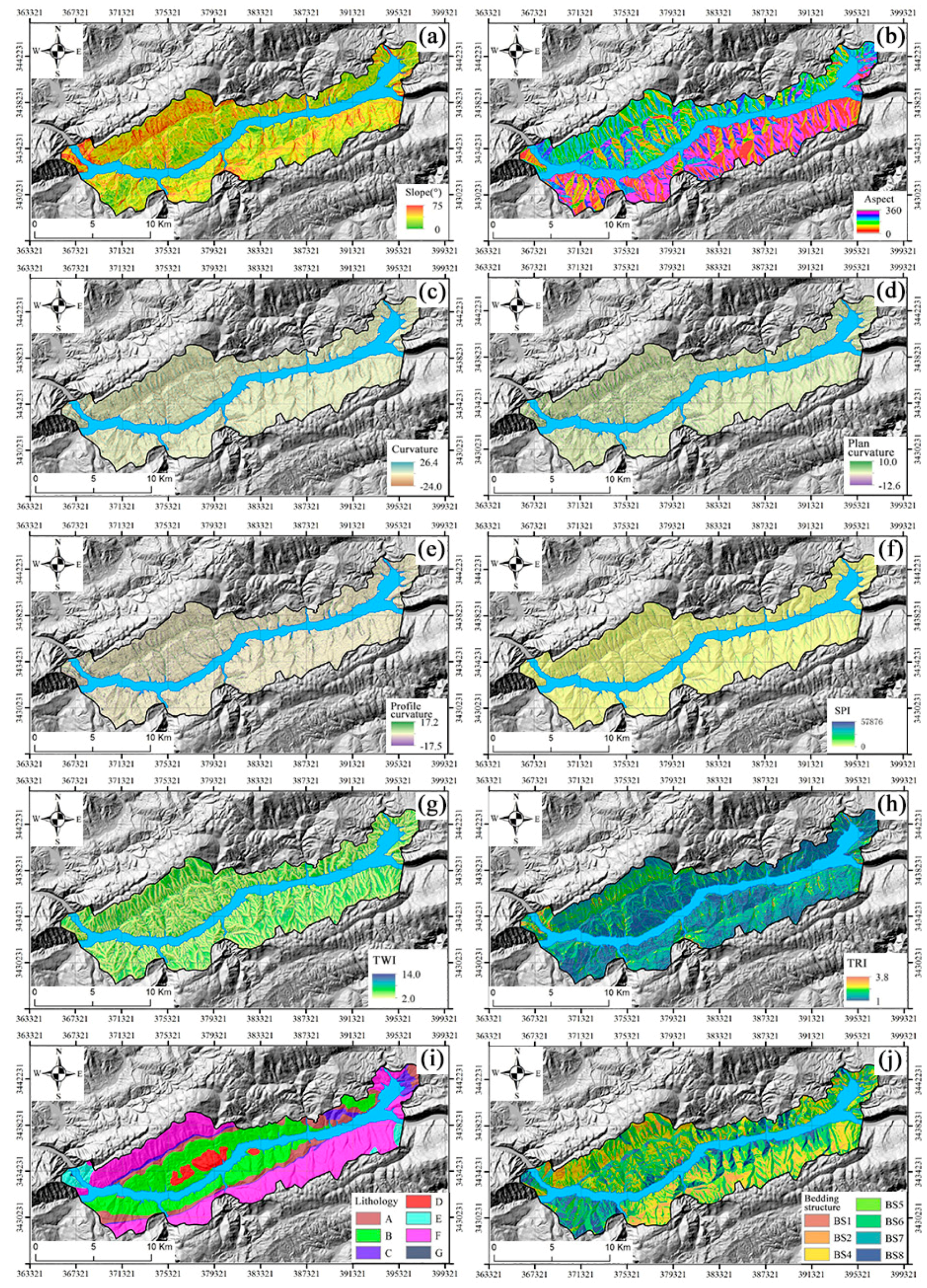
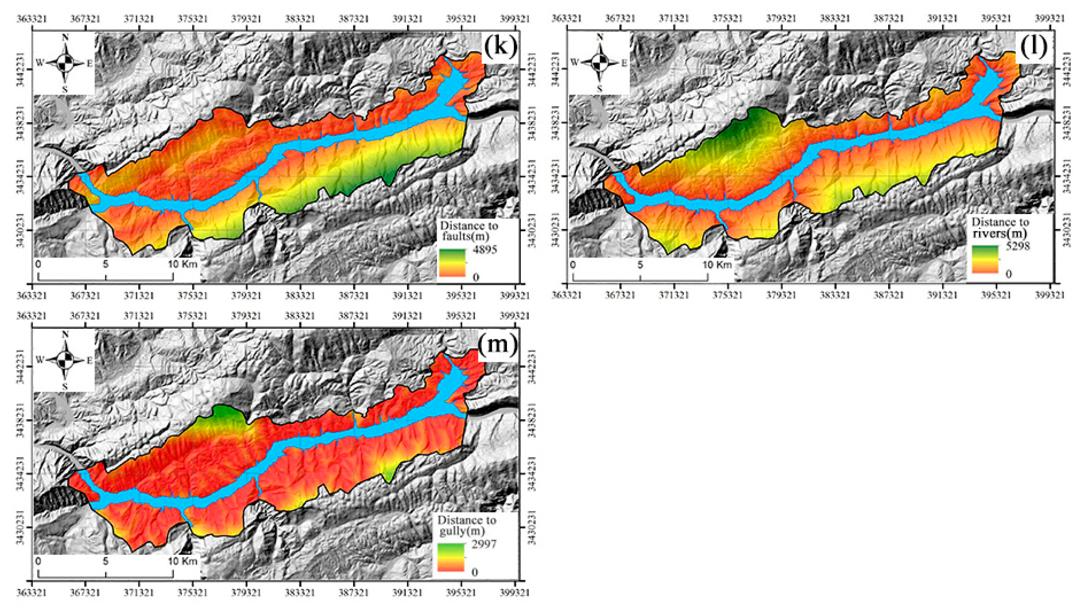
2.3.2. Landslide Causal Factors

The occurrence of a landslide is caused by the combination of the basic geological conditions of the slope and the external environmental factors. The former are factors that play a controlling role in the occurrence of a landslide, including topography and geological structures, among other factors. The latter are triggering factors for the occurrence of a landslide, such as hydrogeological environment, earthquake, and human engineering activities, among others [28]. According to the field survey and preliminary research results in TGRA [29,30,31], 14 causal factors were initially selected as the factors for landslide susceptibility modelling, including altitude, slope, aspect, curvature, plan curvature, profile curvature, stream power index (SPI), topographic wetness index (TWI), terrain roughness index (TRI), lithology, bedding structure, distance to faults, distance to rivers, and distance to gully. The factors were prepared using a digital elevation model (DEM) with a spatial resolution of 25 m, and geological and geomorphology maps, which were collected from the Chongqing Natural Resources Bureau. In this study, ArcGIS 10.2 (http://www.esrichina.com.cn/) was applied to process geodata, and slope and aspect was obtained by Three Dimensions spatial analysis function; SPI and TWI were calculated by hydrological analysis function and the Raster calculator, respectively. TRI was also calculated using the Raster calculator, and distance to rivers, distance to gully, and distance to faults were calculated using the Euclidean distance method. The continuous causal factors, such as altitude, should be discretized before modelling. The discretization method of continuous landslide causal factors proposed by Zhou et al [32] was utilized in this study.
1. Altitude
The altitude range of the study area is 145–1800 m (Figure 1), which is divided into four levels by the discretization method of continuous causal factors: [145, 300), [300, 450), [450, 750), [750, 1800]. As shown in Table 1, landslides in this study area mainly developed within the altitude from 145 to 300 m, its information value is the highest of 1.752. In the area where the altitude is higher than 750 m, there has been no landslide occurrence, and its information value is −∞.
2. Slope
The slope of the study area varied greatly, mainly from 0° to 75° (Figure 2a), the slope is divided into six levels: [0,6°), [6°,15°), [15°,24°), [24°,33°), [33°,51°) and [51°,75°]. Nearly 55% of the landslides were located in the [6°,15°) and [15°,24°) areas, and their information values were 1.102 and 0.572, respectively. When the slope becomes steep, landslides do not easily occur in this area, with the information value in the [51°,75°] area being −6.306 (Table 1).
3. Aspect
In this study area, aspect can be divided into eight categories (Figure 2b). According to the statistical data, the probability of landslide occurrence on the southeast slope was the largest (Table 1). Its information value was 0.297.
4. Curvature
The curvature of the study area ranged from −24 to 27 (Figure 2c), and it was divided into four categories: [−24,−1), [−1,3), [3,7), and [7,27], their information value being −2.849, 3.668, 2.561, and −0.032, respectively. It can be seen from the calculation results that the information values of the curvatures [1,3) and [3,7) were relatively larger (Table 1), having a promoting effect on the development of a landslide.
5. Plan curvature
The variation range of plan curvature in the study area was −13.0 ~ 10.5 (Figure 2d); it was divided into outward slope [−13, −1.5), straight slope [−1.5,1.5), and inward slope [1.5,10.5], and their information values were −0.566, 0.035, and −0.795, respectively (Table 1).
6. Profile curvature
The variation range of profile curvature in the study area was −18 ~ 18 (Figure 2e); according to the profile curvature, the slope pattern can be divided into convex [−18,−1.5), flat [−1.5,1.5), and concave [1.5,18], and the information values were −0.907, 0.041, and −0.737, respectively (Table 1).
7. SPI
Stream power index can quantitatively describe the relationship between water erosion and land performance [33]. It is usually considered as one of the factors affecting slope stability. The calculation formula is as follows:
S P I = A S tan β
where As is the catchment area of the basin and β is the slope. The SPI can be divided into four categories (Figure 2f): [0,2), [2,4), [4,8), [8, +∞); their information values were 0.262, −0.020, −0.327, and −0.436, respectively (Table 1).
8. TWI
Topographic wetness index can quantitatively simulate the dry and wet conditions of topography and soil moisture in the watershed [33]. The calculation formula is as follows:
T W I = In ( α t a n β )
where α is the upstream convergence area and β is the slope. The TWI can be divided into four categories (Figure 2g): [0,4.5), [4.5,6.5), [6.5,8), and [8, +∞); their information values were 0.047, −0.158, 0.069, and −0.292, respectively (Table 1).
9. TRI
Terrain roughness index (TRI) is an index reflecting the change of surface fluctuation. TRI ranges from 1 to 3.9, and the main range is 1 to 1.2, which accounts for about 70% of the total area of the study area. The continuous factors classified method was applied to classify TRI into four categories (Figure 2h): [1,1.2), [1.2,1.4), [1.4,1.6), and [1.6,3.9]; their information values were 0.338, −1.167, −2.291, and −6.780, respectively (Table 1).
10. Lithology
Lithology is the material basis for the development of a landslide. According to the lithological characteristics of outcropping strata in the study area, they can be divided into seven categories (Table 2), and their spatial distribution is shown in Figure 2i. Nearly 60% of the landslides in the study area developed in category B, and its information value was 0.849 (Table 1).
11. Bedding structure
According to “Technical Requirements for Investigation and Evaluation of Collapse, Landslide, Debris Flow” from the China Geological Survey [34], slope structure can be classified into eight categories (Figure 2j; Table 3), and the statistical results of the information value of each slope structure type are shown in Table 1.
12. Distance to faults
Usually, there are many cracks near the structure, and the rock mass is broken, which provides a material basis for a landslide and is also the area where a landslide is more developed. Distance to faults can be divided four categories (Figure 2k): [0,450), [450,900), [900,1750), and [1750, 4900]; their information values were 0.575, 0.532, −0.611, and −4.311, respectively (Table 1).
13. Distance to rivers
The study area is situated on both sides of the Three Gorges Reservoir, and the river system is the Yangtze River and its main tributaries. The influence intensity is expressed by the distance to rivers. The distance to rivers was divided into six categories (Figure 2l): [0,150), [150,300), [300,650), [650,950), [950,1550), and [1550,5300]. Statistical results showed that the development of landslides in the study area was significantly affected by rivers; 62% of landslides are within 300 m of the Yangtze River, and the farther away from rivers, the fewer landslides developed. When the ranges of the distance to rivers were [0,150) and [150,300), the information values were the largest, being 1.910 and 1.333, respectively (Table 1).
14. Distance to gully
The gully can erode the foot of the slope on the two banks. The distance to the gully was used to characterize its action intensity, which was divided into five grades (Figure 2m): [0,150), [150,350), [350,500), [500,900), and [900,3000]. The gully can promote the development of a landslide. When the ranges of the distance to the gully were [0,150) and [150,350), the information values were 0.285 and 0.182, respectively (Table 1).

2.4. Landslide Causal Factors Selection

2.4.1. Multicollinearity Analysis

Before susceptibility modelling, it is necessary to check whether there is collinearity between the causal factors. In this study, the variance inflation factors (VIF) and the tolerances were used to test the multicollinearity among these 14 factors. When the VIF was ≥5, or the tolerance was ≤0.2, the factor had a collinearity problem. Otherwise, there was no collinearity. As shown in Table 4, the VIF and tolerance of altitude were 0.176 and 5.687, respectively, and the VIF and tolerance of distance to rivers were 0.235 and 4.259, respectively. This means that there was collinearity between altitude and distance to rivers. Thus, it was necessary to remove altitude from the factor system. After removing altitude, the minimum tolerance and maximum VIF were 0.522 and 1.914, respectively (Table 4). There was no collinearity among the new landslide causal factors.

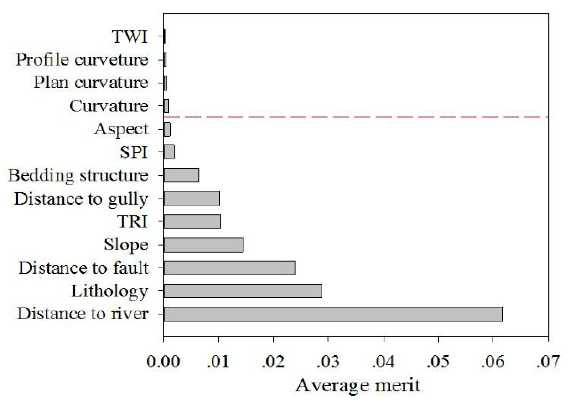
2.4.2. Factor Selection Using Information Gain Ratio

After removing altitude, the importance of each factor in the modelling was quantitatively calculated using IGR, and the results are shown in Figure 3. According to the methodology of IGR in Section 3.1, the factor with larger average merit value made greater contributions to the accuracy of the susceptibility model. The calculation results of IGR showed that distance to rivers was the dominant causal factor in the study area, and its average merit value was 0.061.
Support vector machine has many advantages, such as a stable result and fast operation speed; thus, it was used to test the prediction accuracy of different factor combinations, and the accuracy was calculated using receiver operating characteristic [35]. As shown in Table 5, when eliminating TWI, curvature, plan curvature, and profile curvature, the accuracy of susceptibility modelling was the highest of 0.922. However, when the aspect was excluded, the accuracy of susceptibility modelling was significantly reduced to 0.908. The elimination of inconsequential factors can improve the accuracy of susceptibility modelling. Finally, nine important causal factors were selected for susceptibility modelling.

3. Results and Accuracy Analysis

3.1. Landslide Susceptibility Modelling

In the susceptibility mapping, landslide susceptibility index was considered for the probability of landslide occurrence (landslide: 1, non-landslide: 0). Before landslide susceptibility modelling, the data of landslide causal factors should be normalized. In this study, we normalized the factors into the range of [0.01, 0.99] on the basis of their information values. The normalized value was used as input data, whereas the susceptibility index was used as output data.
In order to test the performance of the used methods, the landslide locations were randomly divided into two parts. A total of 50% of the landslide locations were utilized for the training model, and the remaining 50% were applied to verify the model performance. In the training process of the models, too much or too little training data of any kind would lead to the imbalance of model training. Therefore, the same number of data was randomly selected from the non-landslide area as the training samples. Three machine learning models (SVM, ANN, and CART) and the multivariate statistical model (LR) were used for landslide susceptibility modelling with nine important causal factors. The modelling process of the four models was completed in Clementine 12.
Furthermore, the parameters of SVM and ANN were obtained by error and trial algorithm (Table 6). The CART model did not need any parameter in modelling. In the LR model, the formula of LR model for calculating the landslide susceptibility index (LSI) was as follows:
L S I = ( 6.651 ) + ( SPI ( 0.055 ) ) + ( TRI 1.826 ) + ( Lithology 1.417 ) + ( Slope 1.458 ) + ( Gully 0.806 ) + ( Aspect 0.384 ) + ( River 3.792 ) + ( Faults 0.174 )
The landslide susceptibility index was calculated by SVM, ANN, CART, and LR model, and then was divided into four levels: high (20%), moderate (20%), low (20%) and very low (40%), respectively. The results are shown in Figure 4.

3.2. Accuracy Statistic

In order to validate the modelling accuracy of the used models, the landslide distribution in each susceptibility level was statistically analyzed, and the results are shown in Table 7.
In the SVM model, 88.69% of landslides were located in areas of high susceptibility level, whereas the results of ANN, LR, and CART models were 69.79%, 68.78%, and 62.51%, respectively. Furthermore, the area of high level in SVM model accounted for 20.01% of the total area, but the area of landslide accounted for 88.69% of the entire landslide area, and its frequency ratio was as high as 4.432. The frequency ratios of the other three models were lower than that of the SVM model. ANN and LR models were 3.517 and 3.503, respectively, and the CART model was the lowest of 3.309.
In practical engineering applications, if the area of very low level is misclassified into the area of high level, it will limit effective land-use. However, if the area of high level is misclassified into the area of very low level, it may bring economic losses and casualties in the area. However, the effects of these two cases on the accuracy statistics are the same. Further analysis showed that the area of very low level of SVM model accounted for 40% of the total study area, but its landslide only accounted for 0.02% of the entire landslide area. Its frequency ratio was the lowest of 0.001, which was much lower than those of ANN, LR, and CART models, with those being 0.040, 0.038, and 0.048, respectively.
By comparing the accuracy statistics of the four models, we can see that the SVM model had the highest classification accuracy in the area of high level and the lowest misclassification in the area of very low level, showing better prediction performance.

3.3. Using ROC Curve

Receiver operating characteristic (ROC) curve can effectively analyze the performance of the landslide susceptibility models [36], which can overcome the error caused by setting breakpoints in advance to reclassify the susceptibility index. ROC curves are plotted by taking the false positive rate (sensitivity) of different cut-off thresholds as the y-axis and the real positive rate (specificity) as the x-axis. The area under the ROC curve (AUC) is the area between the curve and the axis, and its value is between 1.0 and 0.5; the closer the value of AUC is to 1, the better the classification effect of the model. The ROC curves of training and verifying performance of the used models are shown in Figure 5.
In model training, the AUC of the SVM model was 0.927, which was better than the ANN, LR, and CART models of 0.866, 0.860, and 0.842 (Table 8), respectively. It was indicated that the SVM model can more accurately fit the nonlinear relationship between landslide occurrence and its causal factors. In model verifying, the predictive performance of the SVM model was also superior, with the highest AUC of 0.922, which was better than the ANN, LR, and CART of 0.875, 0.863, and 0.837, respectively (Table 8).
From the above two methods of accuracy analysis, we can see that the SVM model had the best prediction performance in the susceptibility modelling of the study area, followed by ANN and LR models, and CART had the worst prediction performance.

4. Discussion

In this study area, landslides mainly occurred along the Yangtze River, with an elevation from 145 to 300 m. When the altitude was higher than 750 m, there were no landslides. The distance to rivers (<300 m) and lithology (T2b3, T2b4) had a positive effect on landslides in this area, and their average merit values were 0.061 and 0.029, respectively (Figure 3). A total of 62% of the landslides were within 300 m from the Yangtze River, and nearly 60% of the landslides were with the stratigraphic lithology of T2b3 and T2b4, which were regarded as the main stratum of landslide in the TGRA [37].
The landslide development laws vary in different landslide-prone areas, hence the susceptibility models often perform in varied ways in different regions. In this study, we wanted to find an effective model in TGRA, and thus three machine learning models (SVM, ANN, and CART) and one multivariate statistical model (LR) were utilized. The results showed that the SVM model performed the best (Table 8). At the same time, the SVM performance behavior for susceptibility modelling in other regions were collected. As shown in the literature (Table 9), the accuracy of SVM was always larger than 0.8. We could see that SVM performed acceptably in different regions, and thus it can be used as a recommended model in TGRA and other landslide-prone regions.
In this study, 14 causal factors were preliminarily selected for susceptibility modelling. On the basis of the analysis of the IGR model, the factors could be grouped into the noise factors and the crucial factors. When the noise factors (TWI, curvature, plan curvature, and profile curvature) were removed, the accuracy of the model was gradually improved, but when the crucial factor was eliminated, the accuracy of the model was greatly reduced (Table 5). In this study area, distance to rivers was the most important factor, and the impoundment of the TGRA impacted the landslide development in three aspects: (1) the long-term immersion of reservoir water gradually reducing the strength of rock (soil) at the saturated zone (mostly near the Yangtze river), reducing the resistance force of landslide; (2) the strong dynamic action of water enhancing the lateral erosion on the bank slope, changing the slope shape, and thus reducing the slope stability; (3) the periodic fluctuation of the reservoir water making the self-weight, static, and dynamic water pressure of the landslide change, which could increase the resistance force or reduce the sliding force of the landslide and even cause overall instability and damage [41,42,43,44]. Hence, in order to reduce the losses caused by landslides in TGRA, we should pay more attention to the early warning of reservoir bank landslides.

5. Conclusions

This paper takes Wushan segment in the TGRA as a case study, contributing to a systematic comparison and evaluation of four models for landslide susceptibility modelling. According to this case study, the following results can be noticed: (1) landslide development in the study area is mainly affected by distance to rivers and stratum lithology (T2b3 and T2b4); (2) IGR is an effective method for evaluating the importance of landslide indicators, and eliminating the less important factors can effectively improve the prediction accuracy in landslide susceptibility modelling; and (3) the SVM model shows the best performance in this study area, and thus it can be recommended for susceptibility modelling in TGRA and other landslide-prone regions.

Author Contributions

All authors would like to describe the contributions in detail as follows: conceptualization, L.Y. and C.Z.; data curation, L.Y. and Y.C.; writing—original draft preparation, L.Y. and C.Z.; writing—review and editing, L.Y., C.Z., Y.C., Y.W., and Z.H.; supervision, C.Z. and Y.W.; funding acquisition, C.Z., Y.W., and Y.C.

Funding

This research was funded by the National Natural Science Foundation of China (no. 41907253, no. 41572289, no. 41702330) and the China Geological Survey Projects (no. 000121 2018C C60 003).

Acknowledgments

We greatly appreciate the careful reviews and thoughtful suggestions by reviewers.

Conflicts of Interest

The authors declare no conflict of interest.

References

  1. Yu, M.; Huang, Y.; Zhou, J.; Mao, L. Modeling of landslide topography based on micro-unmanned aerial vehicle photography and structure-from-motion. Environ. Earth Sci. 2017, 76, 520. [Google Scholar] [CrossRef]
  2. Avelar, A.S.; Netto, A.L.C.; Lacerda, W.A.; Becker, L.B.; Mendonça, M.B. Mechanisms of the Recent Catastrophic Landslides in the Mountainous Range of Rio de Janeiro, Brazil; Springer: Berlin/Heidelberg, Germany, 2013; pp. 265–270. [Google Scholar]
  3. Fan, X.; Xu, Q.; Scaringi, G.; Dai, L.; Li, W.; Dong, X.; Zhu, X.; Pei, X.; Dai, K.; Havenith, H.-B. Failure mechanism and kinematics of the deadly June 24th 2017 Xinmo landslide, Maoxian, Sichuan, China. Landslides 2017, 14, 2129–2146. [Google Scholar] [CrossRef]
  4. Cui, P.; Zhou, G.G.D.; Zhu, X.H.; Zhang, J.Q. Scale amplification of natural debris flows caused by cascading landslide dam failures. Geomorphology 2013, 182, 173–189. [Google Scholar] [CrossRef]
  5. National Geological Disaster Bulletin. Available online: http://www.cigem.cgs.gov.cn/gzdt_4839/dwdt_4861/201904/t20190417_479382.html (accessed on 17 April 2019).
  6. Wang, F.; Zhang, Y.M.; Huo, Z.T.; Peng, X.M.; Wang, S.M.; Yamasaki, S. Mechanism for the rapid motion of the Qianjiangping landslide during reactivation by the first impoundment of the Three Gorges Dam reservoir, China. Landslides 2008, 5, 379–386. [Google Scholar] [CrossRef]
  7. Xu, G.L.; Li, W.N.; Yu, Z.; Ma, X.H.; Yu, Z.Z. The 2 September 2014 Shanshucao landslide, Three Gorges Reservoir, China. Landslides 2015, 12, 1169–1178. [Google Scholar] [CrossRef]
  8. Cascini, L. Applicability of landslide susceptibility and hazard zoning at different scales. Eng. Geol. 2008, 102, 164–177. [Google Scholar] [CrossRef]
  9. Corominas, J.; van Westen, C.; Frattini, P.; Cascini, L.; Malet, J.P.; Fotopoulou, S.; Catani, F.; Van Den Eeckhaut, M.; Mavrouli, O.; Agliardi, F.; et al. Recommendations for the quantitative analysis of landslide risk. Bull. Eng. Geol. Environ. 2014, 73, 209–263. [Google Scholar] [CrossRef]
  10. Bui, D.T.; Tuan, T.A.; Klempe, H.; Pradhan, B.; Revhaug, I. Spatial prediction models for shallow landslide hazards: A comparative assessment of the efficacy of support vector machines, artificial neural networks, kernel logistic regression, and logistic model tree. Landslides 2016, 13, 361–378. [Google Scholar]
  11. Yin, K.L.; Yan, T.Z. Statistical prediction models for slope instability of metamorphosed rocks. In Proceedings of the Landslides, Vols 1-3, Rotterdam, The Netherlands, 10–15 July 1988; pp. 1269–1272. [Google Scholar]
  12. Zhu, C.H.; Wang, X.P.; Soc, I.C. Landslide Susceptibility Mapping: A Comparison of Information and Weights-Of-Evidence Methods in Three Gorges Area; IEEE Computer Society: Los Alamitos, CA, USA, 2009; pp. 342–346. [Google Scholar]
  13. Ayalew, L.; Yamagishi, H. The application of GIS-based logistic regression for landslide susceptibility mapping in the Kakuda-Yahiko Mountains, Central Japan. Geomorphology 2005, 65, 15–31. [Google Scholar] [CrossRef]
  14. Kawabata, D.; Bandibas, J. Landslide susceptibility mapping using geological data, a DEM from ASTER images and an Artificial Neural Network (ANN). Geomorphology 2009, 113, 97–109. [Google Scholar] [CrossRef]
  15. Ermini, L.; Catani, F.; Casagli, N. Artificial Neural Networks applied to landslide susceptibility assessment. Geomorphology 2005, 66, 327–343. [Google Scholar] [CrossRef]
  16. Pradhan, B.; Lee, S. Landslide susceptibility assessment and factor effect analysis: Backpropagation artificial neural networks and their comparison with frequency ratio and bivariate logistic regression modelling. Environ. Modell. Softw. 2010, 25, 747–759. [Google Scholar] [CrossRef]
  17. Xu, C.; Dai, F.C.; Xu, X.W.; Lee, Y.H. GIS-based support vector machine modeling of earthquake-triggered landslide susceptibility in the Jianjiang River watershed, China. Geomorphology 2012, 145, 70–80. [Google Scholar] [CrossRef]
  18. Peng, L.; Niu, R.Q.; Huang, B.; Wu, X.L.; Zhao, Y.N.; Ye, R.Q. Landslide susceptibility mapping based on rough set theory and support vector machines: A case of the Three Gorges area, China. Geomorphology 2014, 204, 287–301. [Google Scholar] [CrossRef]
  19. Yao, X.; Tham, L.G.; Dai, F.C. Landslide susceptibility mapping based on Support Vector Machine: A case study on natural slopes of Hong Kong, China. Geomorphology 2008, 101, 572–582. [Google Scholar] [CrossRef]
  20. Marjanovic, M.; Kovacevic, M.; Bajat, B.; Vozenilek, V. Landslide susceptibility assessment using SVM machine learning algorithm. Eng. Geol. 2011, 123, 225–234. [Google Scholar] [CrossRef]
  21. Everitt, B.S. Classification and Regression Trees. In Encyclopedia of Statistics in Behavioral Science; John Wiley & Sons, Ltd.: Hoboken, NJ, USA, 2005. [Google Scholar] [CrossRef]
  22. Pradhan, B.; Lee, S. Regional landslide susceptibility analysis using back-propagation neural network model at Cameron Highland, Malaysia. Landslides 2010, 7, 13–30. [Google Scholar] [CrossRef]
  23. Pham, B.T.; Bui, D.T.; Dholakia, M.B.; Prakash, I.; Pham, H.V.; Mehmood, K.; Le, H.Q. A novel ensemble classifier of rotation forest and Naive Bayer for landslide susceptibility assessment at the Luc Yen district, Yen Bai Province (Viet Nam) using GIS. Geomat. Nat. Hazards Risk 2017, 8, 649–671. [Google Scholar] [CrossRef]
  24. Shigeo, A. Support Vector Machines for Pattern Classification. In Proceedings of the International Joint Conference on Neural Networks, Washington, DC, USA, 15–19 July 2001; Volume 36, pp. 7535–7543. [Google Scholar]
  25. Tian, Y.Y.; Xu, C.; Hong, H.Y.; Zhou, Q.; Wang, D. Mapping earthquake-triggered landslide susceptibility by use of artificial neural network (ANN) models: An example of the 2013 Minxian (China) Mw 5.9 event. Geomat. Nat. Hazards Risk 2019, 10, 1–25. [Google Scholar] [CrossRef]
  26. Kalantar, B.; Pradhan, B.; Naghibi, S.A.; Motevalli, A.; Mansor, S. Assessment of the effects of training data selection on the landslide susceptibility mapping: A comparison between support vector machine (SVM), logistic regression (LR) and artificial neural networks (ANN). Geomat. Nat. Hazards Risk 2018, 9, 49–69. [Google Scholar] [CrossRef]
  27. Budimir, M.E.A.; Atkinson, P.M.; Lewis, H.G. A systematic review of landslide probability mapping using logistic regression. Landslides 2015, 12, 419–436. [Google Scholar] [CrossRef] [Green Version]
  28. Sestras, P.; Bilasco, S.; Rosca, S.; Nas, S.; Bondrea, M.V.; Galgau, R.; Veres, I.; Salagean, T.; Spalevic, V.; Cimpeanu, S.M. Landslides Susceptibility Assessment Based on GIS Statistical Bivariate Analysis in the Hills Surrounding a Metropolitan Area. Sustainability 2019, 11, 23. [Google Scholar] [CrossRef]
  29. Bai, S.B.; Wang, J.; Lu, G.N.; Zhou, P.G.; Hou, S.S.; Xu, S.N. GIS-based logistic regression for landslide susceptibility mapping of the Zhongxian segment in the Three Gorges area, China. Geomorphology 2010, 115, 23–31. [Google Scholar] [CrossRef]
  30. Chen, W.T.; Li, X.J.; Wang, Y.X.; Liu, S.W. Landslide susceptibility mapping using LiDAR and DMC data: A case study in the Three Gorges area, China. Environ. Earth Sci. 2013, 70, 673–685. [Google Scholar] [CrossRef]
  31. Wu, X.L.; Niu, R.Q.; Ren, F.; Peng, L. Landslide susceptibility mapping using rough sets and back-propagation neural networks in the Three Gorges, China. Environ. Earth Sci. 2013, 70, 1307–1318. [Google Scholar] [CrossRef]
  32. Zhou, C.; Yin, K.L.; Cao, Y.; Ahmed, B.; Li, Y.Y.; Catani, F.; Pourghasemi, H.R. Landslide susceptibility modeling applying machine learning methods: A case study from Longju in the Three Gorges Reservoir area, China. Comput. Geosci. 2018, 112, 23–37. [Google Scholar] [CrossRef] [Green Version]
  33. Moore, I.D.; Grayson, R.B.; Ladson, A.R. Digital terrain modelling: A review of hydrological, geomorphological, and biological applications. Hydrol. Process. 1991, 5, 3–30. [Google Scholar] [CrossRef]
  34. Technical Requirements for Investigation and Evaluation of Collapse, Landslide, Debris Flow. Available online: http://www.mnr.gov.cn/gk/bzgf/201004/t20100406_1971713.html (accessed on 6 April 2010).
  35. Bui, D.T.; Lofman, O.; Revhaug, I.; Dick, O. Landslide susceptibility analysis in the Hoa Binh province of Vietnam using statistical index and logistic regression. Natural Hazards 2011, 59, 1413–1444. [Google Scholar] [CrossRef]
  36. Hanley, J.A.; McNeil, B.J. A method of comparing the areas under receiver operating characteristic curves derived from the same cases. Radiology 1983, 148, 839–843. [Google Scholar] [CrossRef]
  37. Miao, H.; Wang, G.; Yin, K.; Kamai, T.; Li, Y. Mechanism of the slow-moving landslides in Jurassic red-strata in the Three Gorges Reservoir, China. Eng. Geol. 2014, 171, 59–69. [Google Scholar] [CrossRef] [Green Version]
  38. An, K.; Niu, R. Landslide Susceptibility Assessment Using Support Vector Machine Based on Weighted-information Model. J. Yangtze River Sci. Res. Inst. 2016, 33, 47–51. [Google Scholar]
  39. Marjanovic, M.; Bajat, B.; Kovacevic, M. Landslide Susceptibility Assessment with Machine Learning Algorithms; IEEE: New York, NY, USA, 2009; pp. 273–278. [Google Scholar]
  40. Chen, W.; Pourghasemi, H.R.; Panahi, M.; Kornejady, A.; Wang, J.L.; Xie, X.S.; Cao, S.B. Spatial prediction of landslide susceptibility using an adaptive neuro-fuzzy inference system combined with frequency ratio, generalized additive model, and support vector machine techniques. Geomorphology 2017, 297, 69–85. [Google Scholar] [CrossRef]
  41. Bilasco, S.; Horvath, C.; Cocean, P.; Sorocovschi, V.; Oncu, M. Implementation of the usle model using gis techniques. case study the somesean plateau. Carpath. J. Earth Environ. Sci. 2009, 4, 123–132. [Google Scholar]
  42. Zhou, C.; Yin, K.; Cao, Y.; Ahmed, B. Application of time series analysis and PSO–SVM model in predicting the Bazimen landslide in the Three Gorges Reservoir, China. Eng. Geol. 2016, 204, 108–120. [Google Scholar] [CrossRef]
  43. Zhou, C.; Yin, K.; Cao, Y.; Intrieri, E.; Ahmed, B.; Catani, F. Displacement prediction of step-like landslide by applying a novel kernel extreme learning machine method. Landslides 2018, 15, 2211–2225. [Google Scholar] [CrossRef] [Green Version]
  44. Tang, H.; Wasowski, J.; Juang, C.H. Geohazards in the three Gorges Reservoir Area, China–Lessons learned from decades of research. Eng. Geol. 2019, 261, 105267. [Google Scholar] [CrossRef]
Figure 1. (a) The location of Three Gorges Reservoir area (TGRA) in China. (b) The location of the study area. (c) Elevation map of the study area with landslide distribution (the landslides polygons were obtained from historical landslide data, field investigation, and high-resolution remote sensing image data).
Applsci 09 04756 g001
Figure 2. Landslide causal factors of the study area: (a) slope, (b) aspect, (c) curvature, (d) plan curvature, (e) profile curvature, (f) SPI, (g) TWI, (h) TRI, (i) lithology, (j) bedding structure, (k) distance to faults, (l) distance to rivers, (m) distance to gully.
Applsci 09 04756 g002aApplsci 09 04756 g002b
Figure 3. The average merit of each causal factor.
Applsci 09 04756 g003
Figure 4. Landslide susceptibility maps obtained from (a) ANN model, (b) logistic regression (LR) model, (c) SVM model, and (d) classification and regression tree (CART) model.
Applsci 09 04756 g004
Figure 5. The receiver operating characteristic (ROC) curves of the SVM, ANN, LR, and CART models in landslide susceptibility assessment: (a) training and (b) verifying.
Applsci 09 04756 g005
Table 1. Spatial relationships between causal factors and landslides.
Causal FactorCategoryPixels in LandslidePixels in TDProportion of LTLProportion of DTDIVNC
Altitude (m)<30017,32481,07168.7120.411.7520.990
300–450604986,45223.9921.760.1410.663
450–7501839113,5187.2928.57−1.9700.337
>7500116,248029.26−∞0.01
Slope (°)<653883422.132.100.0230.598
6–15419630,80616.647.751.1020.99
15–249711102,94838.5225.910.5720.794
24–337608129,12330.1832.50−0.1070.402
33–513153118,58912.5129.85−1.2550.206
51–75674810.021.88−6.3060.01
Aspect (°)0–45342745,38813.5911.420.2510.849
45–90236339,5979.379.97−0.0890.283
90–135338043,36813.4110.920.2960.99
135–180406760,12816.1315.130.0920.707
180–225205844,7408.1611.26−0.4640.01
225–270175033,8246.948.51−0.2950.141
270–315318050,72712.6112.77−0.0180.424
315–360498779,51719.7820.01−0.0170.566
Curvature−24 to −13254369,40212.9192.98−2.8490.01
−1 to 321,57726,74985.586.733.6680.99
3–73729931.480.252.5620.663
7–2791450.040.04−0.0320.337
Plan curvature−13 to −1.556213,1062.233.30−0.5660.5
−1.5 to 1.524,231372,72596.1193.820.0350.99
1.5–10.541911,4581.662.88−0.7950.01
Profile curvature−18 to −239711,7321.572.95−0.9070.01
−2 to 224,319372,53596.4693.770.0410.99
2–1849613,0221.973.28−0.7360.5
Stream power index (SPI)0–213,724180,39154.4345.410.2620.99
2–4430468,74617.0717.30−0.0200.663
4–8319663,15912.6815.90−0.3270.337
>8398884,99315.8221.39−0.4360.01
Topographic wetness index (TWI)0–4.518,990289,61475.3272.900.0470.663
4.5–6.5485685,39119.2621.49−0.1580.337
6.5–8.595414,3353.783.610.0690.99
>8.541279491.632.00−0.2920.01
Terrain roughness index (TRI)1–1.222,324278,27488.5570.040.3380.99
1.2–1.4264593,56210.4923.55−1.1670.663
1.4–1.623918,4310.954.64−2.2910.337
Distance to rivers (m)>1.6470220.021.77−6.8000.01
0–150995841,76739.5010.511.9100.99
150–300565935,39622.458.911.3330.794
300–650504767,80120.0217.070.2300.598
650–950225947,0968.9611.85−0.4040.402
950–1550180869,7767.1717.56−1.2920.206
>1550481135,4531.9134.09−4.1600.01
Distance to gully (m)0–15015,036194,53659.6448.970.2840.99
150–3507653106,28930.3526.750.1820.75
350–500155330,9016.167.78−0.3370.5
500–90096236,0223.829.07−1.2490.26
>900829,5410.037.44−7.8720.01
Distance to faults (m)0–45014,652154,95958.1239.000.5750.99
450–900712177,60728.2419.530.5320.663
900–1750315575,91412.5119.11−0.6110.337
>175028488,8091.1322.35−4.3110.01
Lithology (L)L1389047,61215.4311.980.3650.598
L215,126132,29960.0033.300.8490.794
L3131620,2095.225.090.0370.402
L4200316,3077.944.100.9530.99
L5011,8260.002.98−∞0.01
L62877168,88011.4142.51−1.8970.206
L701560.000.04−∞0.01
Bedding structure (BS)BS12065090.820.132.6730.99
BS2142334,2005.648.61−0.6090.173
BS4320487,21112.7121.95−0.7890.337
BS5469587,74118.6222.08−0.2460.01
BS68549113,52333.9128.570.2470.5
BS7372139,37614.769.910.5740.663
BS8341434,72913.548.740.6310.827
Note: TD = total domain, LTL = landslide in total landslide, DTD = domain in total domain, IV = information value, NC = normalized class.
Table 2. Lithological classification in the study area.
CategoryMain LithologyGeologic Group
ASiltstone, silty mudstoneT2b2
BSiltstone, muddy limestone, dolostone with mudstoneT2b3, T2b4
CMudstone, muddy limestoneT2b1
DSandstone, silty shaleT3xj1, T3e
EMuddy limestone with limestoneT1d1, T1d2, T1d3, T1d4
FLimestone with dolostone, muddy limestone, dolomitic limestoneT1j1, T1j2, T1j3, T1j4
GLimestone, silty shale with coal seamP3w, P3d
Table 3. Classification of bedding structure.
Category Definition   ( slope : θ ,   aspect : σ ,   bed   dip   angle : α ,   bed   dip   direction : β )
BS1 α < 10 °
BS2 ( ( | α β | ( 0 , 30 ° ] ) ( | α β | [ 330 ° , 360 ° ) ) ) & & ( α > 10 ° ) & & ( θ > α )
BS3 ( ( | α β | ( 0 , 30 ° ] ) ( | α β | [ 330 ° , 360 ° ) ) ) & & ( α > 10 ° ) & & ( θ = α )
BS4 ( ( | α β | ( 0 , 30 ° ] ) ( | α β | [ 330 ° , 360 ° ) ) ) & & ( α > 10 ° ) & & ( θ < α )
BS5 ( | α β | [ 30 ° , 60 ° ) ) ( | α β | [ 300 ° , 330 ° ) )
BS6 ( | α β | [ 60 ° , 120 ° ) ) ( | α β | [ 240 ° , 300 ° ) )
BS7 ( | α β | [ 90 ° , 150 ° ) ) ( | α β | [ 210 ° , 240 ° ) )
BS8 ( | α β | [ 120 ° , 180 ° ) ) ( | α β | [ 180 ° , 210 ° ) )
Table 4. Multicollinearity of the causal factors. VIF: variance inflation factors.
FactorOriginal Factor SystemNew Factor System
TolerancesVIFTolerancesVIF
Altitude0.1765.687//
Slope0.5351.8700.5361.867
Aspect0.9791.0210.9801.021
Curvature0.8461.1830.8491.178
Plan curvature0.9261.0800.9271.079
Profile curvature0.8761.1420.8761.142
TRI0.5221.9160.5221.914
Lithology0.4892.0440.5441.837
Bedding structure0.9391.0650.9411.063
Distance to faults0.6031.6580.6271.595
Distance to rivers0.2354.2590.7511.332
Distance to gully0.7691.3000.8021.247
Table 5. The prediction accuracy with elimination of the less important factors.
ModelEliminating Less Important FactorsAccuracy
Model 1Without eliminating any factor0.918
Model 2TWI0.918
Model 3TWI, profile curvature0.920
Model 4TWI, profile curvature, plan curvature0.919
Model 5TWI, profile curvature, plan curvature, curvature0.922
Model 6TWI, profile curvature, plan curvature, curvature, aspect0.908
Table 6. The parameters of support vector machine (SVM) and artificial neural network (ANN) models.
ModelsParametersNotes
SVMc = 20, γ = 1.3c is the penalty factor, γ is the parameter of the kernel function
ANNn = 5, α = 0.9n is the neurons number, α is the momentum
Table 7. Accuracy statistics of the SVM, ANN, LR, and CRAT models.
Susceptibility LevelPixels in LandslidePixels in DomainProportion of LDProportion of LTLProportion of DTDFrequency Ratios
SVM
Very low6154,2750.00%0.02%38.83%0.001
Low21083,6970.25%0.83%21.07%0.040
Moderate263679,8173.30%10.46%20.09%0.520
High22,36079,50028.13%88.69%20.01%4.432
ANN
Very low409160,3780.26%1.62%40.37%0.040
Low174179,1552.20%6.91%19.92%0.347
Moderate547978,9756.94%21.73%19.88%1.093
High17,58378,78122.32%69.79%19.83%3.517
LR
Very low393161,7460.24%1.56%40.71%0.038
Low183879,1272.32%7.29%19.92%0.366
Moderate564078,4117.19%22.37%19.74%1.133
High17,34178,00522.23%68.78%19.63%3.503
CART
Very low491160,3780.31%1.95%40.37%0.048
Low134179,4191.69%5.32%19.99%0.266
Moderate762182,4409.24%30.23%20.75%1.457
High15,75975,05221.00%62.51%18.89%3.309
Note: LD = landslide in domain, LTL = landslide in total landslide, DTD = domain in total domain.
Table 8. The prediction performance comparison.
ModelsArea Under the ROC Curve (AUC)Standard Error95% Confidence Interval
Lower LimitUpper Limit
Training group
SVM0.9270.0020.9230.930
ANN0.8660.0020.9620.871
LR0.8600.0020.8550.864
CART0.8420.0030.8370.847
Prediction group
SVM0.9220.0010.9200.923
ANN0.8750.0010.8730.877
LR0.8630.0010.8600.865
CART0.8370.0010.8350.840
Table 9. The accuracy of SVM model in different areas.
AuthorsStudy AreaAccuracy of SVM
An et al. [38]The Wangzhou segment of the TGRA0.814
Marjanovic et al. [20]The Fruška Gora Mountain (Serbia)0.842
Marjanovic et al. [39]NW (Northwest) slopes of Fruška Gora Mountain, Serbia0.880
Chen et al. [40]Hanyuan county, China0.875
Bui et al. [10]The Son La hydropower basin (Vietnam)0.887
Note: The accuracy refers to the proportion of historical landslide hazard points in high to very high prone areas.

