Computer Vision in Precipitation Nowcasting: Applying Image Quality Assessment Metrics for Training Deep Neural Networks


1
Department of Big Data Science, University of Science and Technology (UST), Daejeon 34113, Korea
2
Research Data Sharing Center, Division of National Science and Technology Data, Korea Institute of Science and Technology Information (KISTI), Daejeon 34141, Korea
*
Author to whom correspondence should be addressed.
†
Current address of affiliation 2: (34141) 245 Daehak-ro, Yuseong-gu, Daejeon, Korea.
Atmosphere 2019, 10(5), 244; https://doi.org/10.3390/atmos10050244
Submission received: 22 April 2019
/
Revised: 26 April 2019
/
Accepted: 26 April 2019
/
Published: 2 May 2019
(This article belongs to the Section Meteorology)
Abstract
:This paper presents a viewpoint from computer vision to the radar echo extrapolation task in the precipitation nowcasting domain. Inspired by the success of some convolutional recurrent neural network models in this domain, including convolutional LSTM, convolutional GRU and trajectory GRU, we designed a new sequence-to-sequence neural network structure to leverage these models in a realistic data context. In this design, we decreased the numbers of channels in high abstract recurrent layers rather than increasing them. We formulated the task as a problem of encoding five radar images and predicting 10 steps ahead at the pixel level, and found that using only the common mean squared error can misguide the training and mislead the testing. Especially, the image quality of last predictions usually degraded rapidly. As a solution, we employed some visual image quality assessment techniques including Structural Similarity (SSIM) and multi-scale SSIM to train our models. Experimental results show that our structure was more tolerant to increasing uncertainty in the data, and the use of image quality metrics can significantly reduce the blurry image issue. Moreover, we found that using SSIM was very effective and a combination of SSIM with mean squared error and mean absolute error yielded the best prediction quality.
1. Introduction
Precipitation nowcasting is one of the most difficult challenges in meteorology, which forecasts rainfall situation in a short range of time (usually from 0.5 to several hours) [1]. In the context of high spatiotemporal resolutions, traditional methods based on the Numerical Weather Prediction model are said to be computationally expensive, too sensitive to noises, highly dependent on initial conditions and not able to exploit big data [2]. Meanwhile, extrapolation-based approaches using radar reflectivity or remote sensing data can provide more accurate prediction [3,4]. Recently, data-driven approaches that leverage advances in machine learning/deep learning have been used to analyze radar images and perform precipitation nowcasting with promising results. Two main branches of this research direction are Radar Echo Extrapolation (REE) and Quantitative Precipitation Forecast (QPF). The former predicts the movements and changes of shape and intensity of precipitation particles in an image sequence [5,6,7], and the latter predicts directly the amount of rainfall in a certain area [8,9]. In the REE tasks, many approaches based-on deep Convolutional Neural Networks (CNNs) and Recurrent Neural Networks (RNNs) have been shown to be better than traditional methods based-on optical flow, such as ROVER [5], TREC and COTREC [7], and Farneback [9]. However, there remains some unresolved issues such as the problem of blurry images which is widely reported.
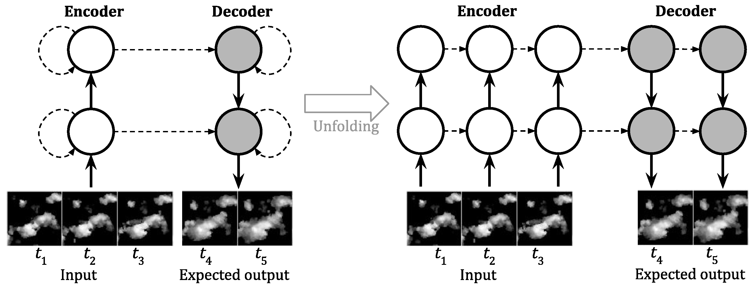
Our study was particularly inspired by the work in [5,6], which led to the emergence of convolutional RNNs (ConvRNNs), including Convolutional Long-Short Term Memory (ConvLSTM [5]), Convolutional Gated Recurrent Unit (ConvGRU [10]) and Trajectory Gated Recurrent Unit (TrajGRU [6]). Their core idea is to replace fully-connected operations in the step-to-step transitions between traditional RNN cells (1D states) by convolutional operations (2D states). This makes ConvRNNs ideal to represent and predict sequential image data, especially radar echo images. Differs from ConvLSTM and ConvGRU, which directly use convolution for the state transitions, TrajGRU uses convolution to generate flow fields of two steps and calculates new states by a warping procedure. We noticed that the operation of TrajGRU is quite similar to three steps of the widely applied numerical McGill algorithm [11,12,13,14]: radar echo tracking, radar reflectivity advecting (by a semi-Lagrangian extrapolation) and error evaluating. However, while this type of traditional method needs predefined spatial filters and translation vector to detect the motions, deep learning methods can automatically learn features from data in an end-to-end fashion [5]. Unlike the traditional calibration with just several events, accessing to a lot of data and patterns can help them to be more tolerant to noises and even uncertainty. Moreover, one can construct ConvRNN models as sequence-to-sequence networks with many stacked layers (Figure 1), and use the convolutional downsampling technique in image processing to build hierarchical structures. This allows ConvRNN models to “see” and predict radar images at different spatial scales, rather than ignoring scale as TREC models [15]. It also allows flexibly extending the input length or prediction lead times, as well as utilize precipitation information from all previous steps rather than using only the current situation like traditional models [16]. Another advantage of deep neural networks is that they can be easily applied for various spatial scales, image sizes and image resolutions, simply by stacking more layers or changing the convolutional kernel sizes. Especially, Shi et al. [6] showed that modifying the training loss function appropriately can increase the accuracy in predicting heavy rainfall events, which is a drawback of McGill models [14].
In this work, we investigated the REE task from a Computer Vision (CV) point of view and suggested some improvements. We adapted the network structure in [6] and compared different test metrics of the three aforementioned convolutional RNNs in a real situation. While TrajGRU is argued to be better than ConvGRU, neither has been studied thoughtfully from an image quality perspective. In addition, even though the prediction quality of ConvGRU is said to be on par with that of ConvLSTM but using less computational resources, a direct comparison between them has not been done in the same context. Our work differs from that in [6] as we estimated the image pixel distribution rather than the reflectivity threshold mapped to each pixel, which allowed us to conveniently apply several Image Quality Assessment (IQA) metrics to guide the training process. We aimed at providing a guidance on choosing an appropriate one among them for future operational researches, especially when previous works still suffered the blurry image problem. Previous works often considered this issue as an inherent uncertainty in the data [5,7]. However, agreeing with Klein et al. [17], we argued that this can be the impact of the loss functions, which mostly based-on L1 or L2 losses (Mean Absolute Error (MAE) or Mean Squared Error (MSE), respectively). Following some works in CV, we hypothesized that using IQA metrics to support the training process could be a very cheap but effective solution. With that purpose, we were not ambitious to conduct a comprehensive work which is able to serve operational purposes. The findings of our work can be helpful in several aspects of our daily life such as aviation management, or prediction of local convective storms, as well as can be used for supporting the QPF tasks [3,7,9,17].
Our contributions are three folds: (1) From a CV viewpoint, we evaluated three popular ConvRNN models in the precipitation nowcasting literature, ConvLSTM, ConvGRU and TrajGRU, and argued that the common practice of using L1/L2 measure for training could mislead the judgment among them. (2) We proposed a new design of the sequence-to-sequence structure to cope with high uncertainty in weather data by reducing the numbers of channels in high abstract layers, namely dec-seq2seq. (3) We investigated the applicability of some IQA metrics and implemented effective loss functions for solving the blurry image issue. To the best of our knowledge, no work has tried this approach in the REE literature.
2. Related Work
For detail information of CNNs and RNNs (applied in precipitation nowcasting), we refer the readers to works by Klein et al. [17] and by Heye et al. [2], Shi et al. [5] and Shi et al. [7], respectively. Here, we summarize d some works leading to our solutions.
2.1. Deep Learning for Radar Echo Extrapolation Based Precipitation Nowcasting
2.1.1. CNN-Based Models
CNNs are originally proposed for analyzing 2D data, but can be used to learn 3D data representation. Hence they are able to analyze 2D radar image sequence, by considering the temporal dimension as the remaining dimension in the 3D representation. Among the first attempts to use CNNs for the REE task is the work in [17], which predicts the center patch of a radar image using a dynamic network with dynamic filters generated by convolving the input images. However, it requires inputting a fixed-length sequence, hence cannot allow flexible sequence length and is not convenient to predict many steps. Later, Shi et al. [7] used a cyclic CNN structure to convolve the final image with features extracted from the input sequence to predict one step ahead. It is shown to be better than traditional methods such as Tracking Radar Echoes by Correlation (TREC) and Continuity of TREC (COTREC). However, these approaches predict only one step ahead in each prediction operation, while our requirement is to make multi-step predictions, which is more important [2], and we targeted to predicting the whole images rather than a certain patch. These approaches can be extended to predict several steps by feeding the predicted image back into the input sequence, but this would make the errors on the output layer accumulate step-by-step [6]. Another CNN-based approach for the same purpose is 3D-CNN [18], but Shi et al. [6] showed that it is not better than their TrajGRU model.
2.1.2. Convolutional RNN-Based Models
The REE task seems to be benefited the most by the family of convolutional RNNs. Firstly, ConvLSTM is introduced in [5] and has caught the attention from many domains. The traditional architecture of LSTM works on 1D vectors of cell’s memory and state, and uses fully-connected operations (matrix multiplication) for operating the gates and state transitions. This is a drawback with 2D data (image or video frames), because the spatial correlation is not exploited and there are too many redundant weights (which make the training process expensive but not effective). With convolutional filters replacing the matrix multiplications, ConvLSTM can preserve and exploit the spatial correlations while representing the temporal correlations simultaneously. Thanks to that, a sequence-to-sequence model built from ConvLSTM cells outperforms the Real-time Optical flow by Variational methods for Echoes of Radar (ROVER) algorithm, which is considered as the state of the art optical flow based model [19].
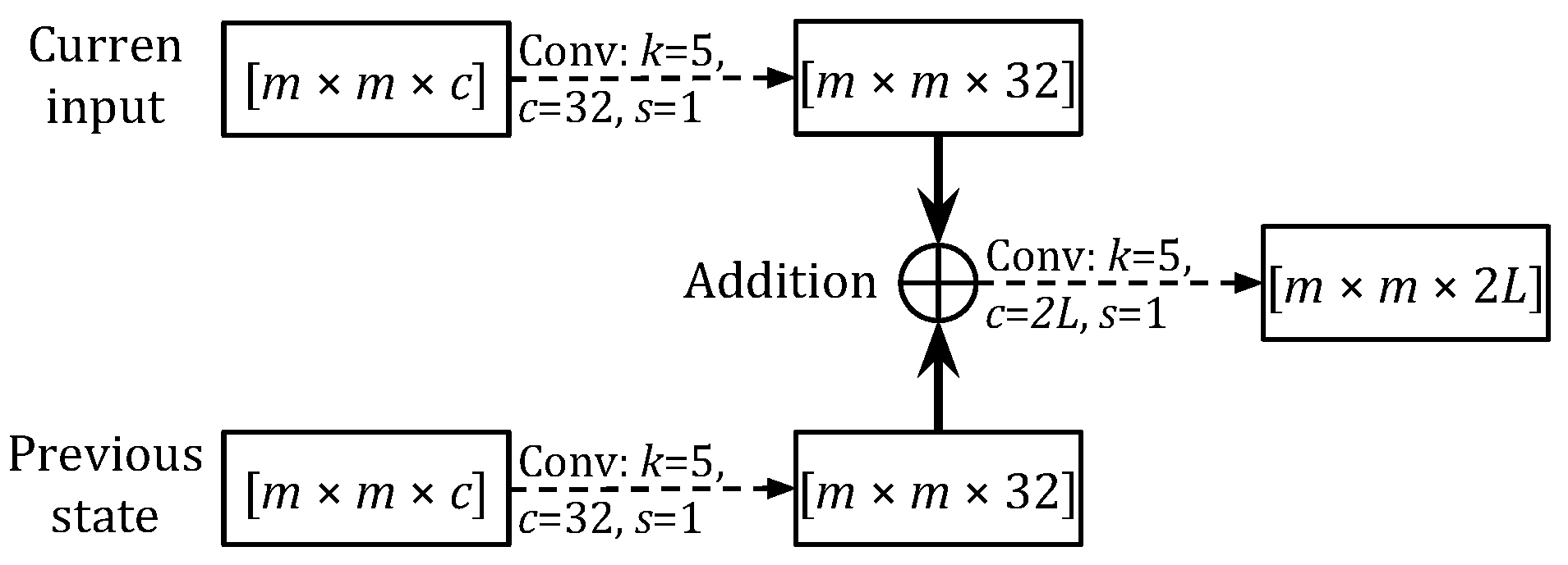
This idea can be generalized to perform the state-to-state transitions in any type of RNNs. Ballas et al. [10] applied it to implement ConvGRU in a video recognition task. These advances have been applied successfully in other domains such as image/video sequence representation [20,21] and abnormal event detection [22]. Later, Shi et al. [6] proposed TrajGRU model based-on the network structure in [10], which outperforms ConvGRU in the same conditions in an REE task. Distinct from ConvGRU and ConvLSTM, which use one filter for different locations (location-invariant), TrajGRU uses a location-variant mechanic which tracks a set of neighbouring points between the input and the previous state. This is done by a sub-network to calculate the optical flow between two consecutive sets of feature maps (Figure 2). This is able to handle complex variations such as rotation or scaling, which are not captured well in ConvGRU and ConvLSTM.
To leverage the power of convolutional RNNs, sequence-to-sequence networks built from stacked multi-layers of cells are usually used to encode an input sequence and produce a predicted sequence [6,10] (Figure 1). Shi et al. [6] stacked three layers of cells to form an encoding-forecasting network. In the encoder, feature maps are extracted (from the input or previous layer’s output) and their sizes are reduced before feeding into the network cells. In the decoder (or forecaster), deconvolutions are used to construct the expected output. Note that the direction of the layer-to-layer transitions in the decoder is opposite to that in the encoder. Thanks to that, there is no need to feed a step output back into the network for predicting the next step, as well as the skip-connection technique. Hence, one of the strongest properties of this encoder–decoder structure is the ability to represent sequences of any lengths, and predict multiple steps ahead. Using this design, Shi et al. [6] was able to use five input steps and predict fifteen consecutive steps ahead. These ConvRNN-based models have been applied successfully in other precipitation nowcasting tasks [1,2,16,23] and other weather forecasts, such as storm tracking [24]. For an REE task, Sato et al. [16] modified ConvGRU network to overcome TrajGRU in [6], but that structure is significantly more complex, and we would leave it for future applications.
Note that some works use the term “Convolutional RNNs” to describe a unified network that consists of separated convolution layers and fully-connected recurrent layers. We do not cover those approaches in this study.
2.1.3. Loss Functions for Training Neural Networks
Most of the previous works report the blurry effect in predicted images. Among the main causes of this issue are the drawbacks of the training loss functions [25]. In fact, they usually used the MSE loss (or L2-based losses) as a default to train their models. Klein et al. [17] used the Euclidean error and argued that it is able to lead to sub-optimal results, in which blurrier images may be penalized less than more natural looking ones. This is because the L2 loss may make a good assumption about the global similarity of two images, but not their local structures. In [7], the same issue appears but is referred as the consequence of the meteorological uncertainty in the atmosphere. The L1 loss function is said to have the same impacts [25,26]. Shi et al. [6] proposed a combination of balanced MSE and MAE based on the precipitation intensity value to enhance the performance on predicting heavy rain. However, we argued that such combination is tricky and still not enough to overcome the issue because it still bases on L1 and L2 only. Singh et al. [23] proposed to use Generative Adversarial Networks and showed promising results. However, this technique is not easy to train and require significant more computing resources. In contrast, IQA metrics are much simpler and less computationally expensive.
In a wider picture of training neural network models in remote sensing, the loss functions have not gained much attention. Most works in this area that study IQA metrics are for the image processing tasks. For example, Palubinskas [27] analyzed the similarities and differences of MSE and SSIM; Xia and Chen et al. [28] mentioned the importance of image quality in meteorology and other remote sensing domains; and Yang et al. [29] stated the same problem for reconstructed hyper-spectral images. However, in tasks related to the image prediction challenge, mostly L1 and/or L2 losses are used as the default training cost measure. We argued that an investigation into this direction could lead to a significant improvement for the REE task. A similar achievement was obtained by Zhao et al. [25] for the image restoration tasks, who argued that combining different loss functions can result in better image quality even though the models are kept unchanged.
2.2. Image Quality Assessment Metrics in Neural Networks
IQA metrics are originally proposed for assessing the degradation of visual quality of images, and recently often used as loss functions in the image generation tasks. Zhao et al. [25] argued that L2 and the Peak Signal to Noise Ratio (PSNR) measure can be misleading because they average the global error in an entire image. They tested the ability of SSIM and MS-SSIM, the two most popular reference-based measures of the IQA literature, for the tasks of image super-resolution, denoising and demosaicking and showed promising results. They suggested, however, that using only SSIM or MS-SSIM will not provide enough error information, and that combining different kinds of loss functions is a better way. Their experiments showed that MS-SSIM+L1 can result in the best quality, while using only L2 can lead to the local optimal problem because of it convergence properties. Palubinskas [27] theoretically analyzed the advantages and drawbacks of MSE and SSIM, and proposed a composite IQA measure by combining Means, Standard deviations and Correlation coefficient. Unfortunately, there was no experimental report on the performance of this measure.
Recently, there have been more complex IQA metrics that take advantages of the extracted feature from the middle layers of neural network. Dosovitskiy and Brox [30] proposed a deep perceptual similarity (DeePSiM) metric to measure the similarity between the extracted abstract features of two images. Then, Lu et al. [31] applied that idea successfully in a combination with the GAN technique for training ConvLSTM models in a video prediction task. Lee et al. [32] used a cosine similarity extracted from pre-trained VGG-network feature space [33] for comparing images and obtained outstanding results. However, as we were searching for a cheap solution, we would leave these methods for the future work.
3. Materials and Methods
3.1. Dataset: Shenzhen Radar Data
We chose a radar echo image dataset from the CIKM AnalytiCup 2017 competition [34]. The purpose of this dataset is for predicting the rainfall amount of the center site of the images [8], but we used it for the multi-step REE task. This dataset contains totally 14,000 sequences of radar reflectivity maps of four elevation angles (0.5 km, 1.5 km, 2.5 km and 3.5 km), covering some neighboring areas of size 101 km × 101 km. Each sequence has 15 time steps recorded in 90 min with an interval of 6 min. Each image is of size 101 × 101 pixels, and the reflectivity values are converted to grayscale ([0, 255]). However, we did not have information to exactly convert the data back to rain-rate values. There are three sample sets: one training set with 10,000 sequences (in two years) and two test sets (Test A and Test B, recorded in the next one year of the training set) with 2000 sequences per set. Because these sets are from different time periods, this sampling mode is more challenging than the cross-validation sampling one. Moreover, we would require the models to predict the whole maps of different areas rather than only the center patch. Our requirement is therefore more challenging than the mentioned previous works.
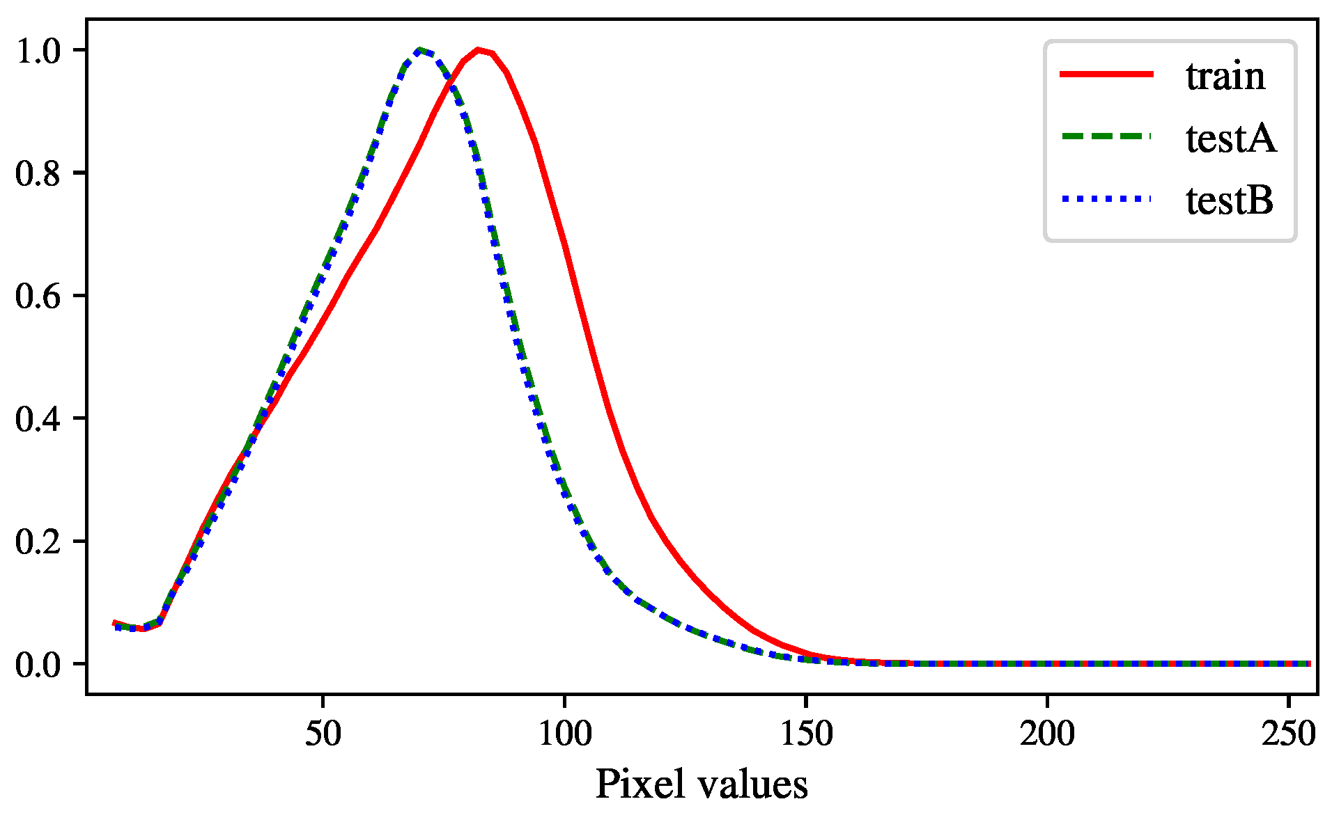
For our purposes, we modified and used the data as follows. We chose only the last channel (at the elevation of 3.5 km), because it has the least missing information or noise. In addition, a prediction of radar images at this elevation can be helpful for the aviation management, which we would aim at in our future projects. Note that we did not interpolate missing data or remove noise, and required the models to deal with these issues inherently. This is another challenge that can figure out which model is better. Finally, we divided each sequence into two parts: the first five steps as the input, and the last ten steps as the ground truth. Unfortunately, we could not extend the length of the sequences as we had no time-stamp information to concatenate them. Figure 3 shows the histograms of data values in the three sample sets (only one channel). The data distribution of the two test sets are significantly different from the training set. This led to a situation that, in a primarily experiment, when we tried using one test set for validating a model trained on the entire training set, its validation error quickly diverged, and the best validation results were too noisy to be recognizable. We believed that this is the most difficult challenge for our study, as well as for practical applications in this domain.
3.2. Sequence-To-Sequence Models for Radar Echo Extrapolation
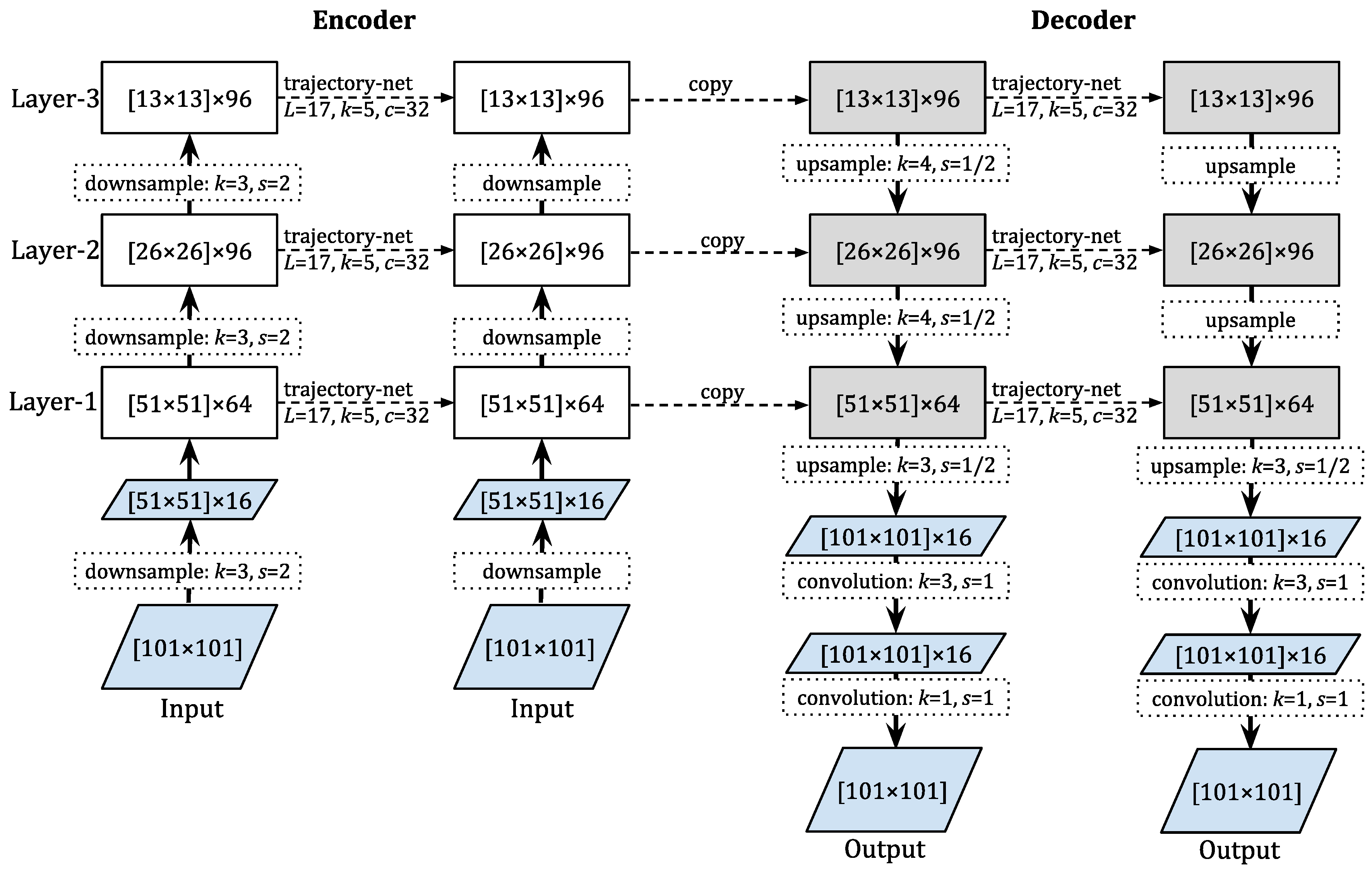
We started by adapting the network structure proposed in [6] to the Shenzhen data. While ConvRNNs methods can be ideal for representing temporal-spatial data, how to design a suitable sequence-to-sequence network is still left opened for research communities. As the image size of the Shenzhen radar data is smaller than the radar images used in [6] (480 × 480 pixels), we chose their smaller configuration used for the MovingMNIST++ task (64 × 64 pixels). This model has three ConvRNN layers incorporated with some convolution and deconvolution layers. The input is of size , and the states are of sizes , and from bottom to top (Figure 4). In the encoder, before the first RNN layer is a convolution layer for down-sampling the original input (by a half) and producing extracted feature maps, which will be the input of the bottom cell. In the decoder, after the bottom ConvRNN cell is one deconvolution layer and two convolution layers to produce the final output. These convolution layers play the role of refining the predicted images.
Regarding to this structure, we realized at least two negative impacts. Firstly, the upsampling operations in the decoder use kernels with size 4 × 4, while all of the downsampling operations use 3 × 3 kernels. This practice makes the encoder and decoder imbalanced in terms of observing resolution and can lead to redundant connections. In fact, we found that using 3 × 3 kernels for all of the downsampling and upsampling operations did not hurt the performance. Secondly, the number of feature maps for representing the states of RNN cells is increased from the bottom layer to the middle layer (from 64 to 96), and kept unchanged at the top layer (96). This is a common practice in the literature. However, we found that it was not helpful in the case where the distributions of training data and testing data are significantly different. Shi et al. [6] dealt with this challenge by using an online-learning strategy, which retrains the models through time when more and more data is coming. However, this solution is not always applicable in the reality, such as when the computing resources for retraining is not available.
Therefore, we proposed to reduce the numbers of feature maps (from 64 to 32 to 16 through bottom-to-top) rather than increasing them. This design was based on a natural intuition widely accepted in Deep Learning that the local correlations can be learned at low abstract feature levels and the global correlations can be learned at higher levels [33]. In the image recognition literature, an increasing the number of channel is needed to ensure that information is not lost too much when down-scaling. However, in the prediction task such as this case-study, preserving too many details could make the models suffer from the over-fitting problem because, at a higher abstraction level, a model is expected to make assumption about the global rather than the local variations, detail information is not needed. Besides this ability, our design has less computing consumption thanks to a smaller number of parameters. We discuss this aspect more clearly in Section 4. Note that Shi et al. [6] used two convolution layers after the last deconvolution, but we found that using only the one with kernel size was enough and could produce finer result. For convenience, we named our structure dec-seq2seq because its main property is decreasing channels from layer to layer.
3.3. Image Quality Assessment Metrics as Training Loss Functions
Besides the commonly used MAE and MSE measures, we followed Zhao et al. [25] in using SSIM and MS-SSIM measures [35,36,37] to implement combined loss functions. For the video predicting task, this practice is employed in [26], which proposes a gradient difference loss function to better capture the fast change between consecutive video frames. However, we found that this gradient-based measure was not helpful in a preliminary experiment with the Shenzhen data, and hence did not consider it in this study. The SSIM method to measure the similarity between two images x and y is defined as follows:
in which is the brightness similarity, is the contrast similarity, and is the structure similarity. and are means of x and y, respectively, while and are standard deviations of x and y, respectively. is the cross correlation of x and y., and are small positive constants for avoiding zero division and numerical instability. All of these items are of a certain local patch rather than the whole image. The image similarity is the average of all local patch similarities. Combining SSIM measures at different scales results in MS-SSIM:
in which , and are relative importance factors, and M is the number of scales. By its nature, MS-SSIM is said to be able to provide more comprehensive evaluation of image difference. In fact, it usually performs better than SSIM in static image processing [25]. We would test if it can provide the same results in the context of an REE task.
For using these measures as loss functions in the neural network training process (that minimizes the training cost), we followed Zhao et al. [25], who defined SSIM and MS-SSIM losses for a pair of predicted and ground truth images as:
To form combined loss functions, we borrowed a simple combination strategy used in [26]:
where l is the component loss chosen in the set {MSE, MAE, SSIM, MS-SSIM} and is the scaling factor for each component.
In addition, for more fairly comparing the outcome of these metrics, we also employed the Pearson Correlation Coefficient (PCC) measure as being used in [38] for remote sensing images. Our models would not be aware of the properties of this measure directly in the training process. Note that we did not employ PSNR, which is commonly used in CV [39], because it would not provide more information when the compared images are of the same range [37].
4. Experimental Results
We conducted several experiments to show that using only MSE and MAE measures to judge models in the context of the REE task is not enough, and our idea to improve the model’s ability of estimating unseen patterns, as well as the effectiveness of some IQA metrics in supporting the training process. We implemented the models with TensorFlow-GPU-1.8 and executed on NVIDIA Tesla P100 GPU (16GB) with the CUDA-9.0 library. All models were trained with the early-stopping strategy and settings in [6] (maximum 200,000 iterations with batch-size 4). We set the learning rate at 0.0001 and decayed it after each 20,000 iterations with a rate of . The pixel values of images were normalized to the range [0.0, 1.0] and all measures of comparison would be calculated on this range. Moreover, to avoid a possible “unlucky” random initialization, we trained each model several times and chose to report the best one here.
4.1. Evaluation of the Previous Work with IQA Metrics
We started by evaluating if a TrajGRU model constructed with the structure in [6] can outperform ConvGRU and ConvLSTM models of the same structure in a viewpoint of CV. In this experiment, the models were trained with only MSE. We randomly selected 8000 samples from the training set for training and used the remaining 2000 samples for validating (to provide the criterion of early stopping). We used all 4000 samples of Test A and Test B sets to form the test set. This scenario is closest to the reality, in which a forecaster observes only the past data for predicting the future. Note that we did not use the Test A or Test B for validating as there was no information about their time periods. We present detail information of the models’ parameters and computing consumption in the training process in Table A1 (Appendix A). Here, we discuss the validating errors and testing measures in Table 1, which interestingly shows different results from different angles. As all models outperformed the basic “last input” technique in all measures by large margins, we would not consider this common baseline again in the following comparisons and analyses.
Firstly, we evaluated the models purely by the MSE measure. On the test set, our results agreed with [6] in that TrajGRU was the best model, with its percentages of advantage over ConvGRU and ConvLSTM were and , respectively. However, even though we found that TrajGRU was usually better in our different training executions (but not always), these margins were modest while the training process is more costly. Moreover, on the validating set, the errors of ConvGRU and ConvLSTM were much better than TrajGRU. This can be explained as the impact of the over-fitting problem was more severe with ConvGRU and ConvLSTM. When they were based on location-invariant filters, it appeared that they could learn well familiar patterns but were not strong in exploring unseen patterns. This explanation was not mentioned in [6], but we believed that this is a critical point to consider when bringing these ConvRNNs models into practical uses. We argued that if the patterns in training and testing data are consistent, ConvGRU and ConvLSTM can be better than TrajGRU.
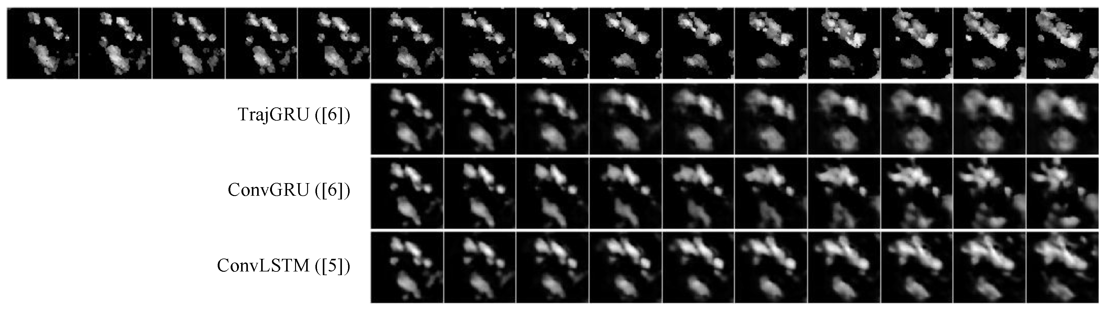
Secondly, in terms of the MAE measure and other IQA metrics, it is clear that TrajGRU was outperformed by ConvGRU and ConvLSTM. Particularly with SSIM, it was and worse than ConvGRU and ConvLSTM, respectively. With MAE, the advantages of ConvGRU and ConvLSTM were and , respectively. This means that TrajGRU is not better than the others in reflecting the local correlations and producing sharp edges of objects. Figure 5 shows an example for demonstrating these findings. Intuitively, TrajGRU produced less accurate estimation of the local shape and resulted in more blurry images. We argued that the reason is because ConvGRU and ConvLSTM use location-invariant filters and hence are able to preserve the local shapes (from the previous step) better, while TrajGRU tends to break the local shapes and make a stronger assumption about global changes between two steps. That was why TrajGRU was better on the MSE measure, which is a global-orienting metric [17]. This trade-off property is not discussed in [6].
Finally, to synthetically compare each couple of models over these metrics, we averaged the percentages of advantage of a model over the other. By this way, ConvGRU and ConvLSTM were and better than TrajGRU, respectively, mainly thanks to their much better SSIM measure. Moreover, ConvGRU was better than ConvLSTM, which confirmed the conclusion in [6] that the two models may have similar performance even though the network size of ConvGRU is much smaller. This means that, from a CV perspective, ConvGRU can be the most effective ConvRNN model in the context of Shenzhen dataset. With this result, together with considering the significant higher resources and time consumption of TrajGRU (see Table A1), we inferred that the performance of TrajGRU would not always be as outstanding as stated in [6]. However, we argued that this situation is not advantageous to all the models, hence we altered the network structure as described in Section 3.2 and were able to produce more reliable predictions in the next experiment.
4.2. Evaluation of the dec-seq2seq Network Structure
We examined the behaviors of TrajGRU, ConvGRU and ConvLSTM models constructed with our proposed structure, and compared them with the above models. We named our models dec-TrajGRU, dec-ConvGRU and dec-ConvLSTM and reused the above training settings. Table 2 presents the validating and testing results, showing improvements of generalization by our design. On the test set, our models significantly improved over MSE, MS-SSIM and PCC. Especially with MSE, dec-TrajGRU, dec-ConvGRU and dec-ConvLSTM improved , and from their previous versions, respectively. With MAE and SSIM, only dec-TrajGRU was able to improve, while dec-ConvGRU and dec-ConvLSTM got worse. Synthetic comparing, dec-TrajGRU was and better than dec-ConvGRU and dec-ConvLSTM, respectively, while dec-ConvGRU was better than dec-ConvLSTM. In addition, our dec-TrajGRU was better than ConvGRU, considered the best model in Section 4.1. Interestingly, the validating error of all models significantly increased. This means that the dec-seq2seq structure was effective in reducing the over-fitting issue, especially for ConvGRU and TrajGRU. It is more impressive to note that our models are almost 3–4 times smaller than the previous ones (see Table A1, Appendix A).
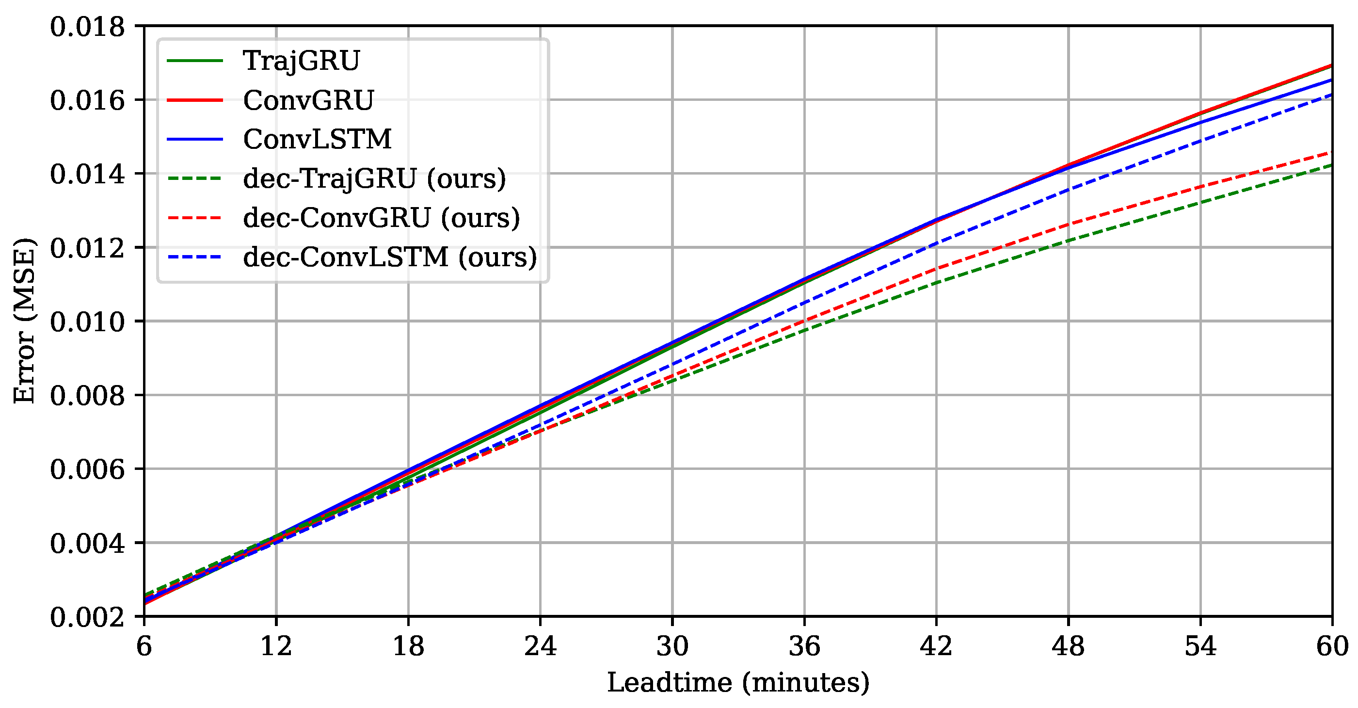
To view the results more clearly, we plotted the lead time errors of six models in Figure 6. It is interesting that all models worked quite similarly on the first two or three steps, but our models significantly outperformed the previous models when going further into the future. This means that our proposed design was more tolerant to the high and increasing uncertainty in the context of Shenzhen dataset. As partly explained in Section 3.2, because our models had less detailed information at the top and middle layers, they were more capable of escaping from familiar patterns (the possible local optimum in the training process) to estimate strange ones at global and intermediate scales better. Moreover, in this viewpoint, dec-TrajGRU is seen as the best model for longer time-step prediction, following by dec-ConvGRU. This means that our proposed design was particularly helpful for the TrajGRU architecture, leveraging its advanced properties successfully in this data context. To confirm this finding, we conducted an extensional experiment to compare TrajGRU and dec-TrajGRU with the MovingMNIST++ data, by generating several test sets with considerably different properties to the training set (see Appendix B). The results were similar: when the uncertainty increased, both models got worse but dec-TrajGRU was less mistaken than TrajGRU.
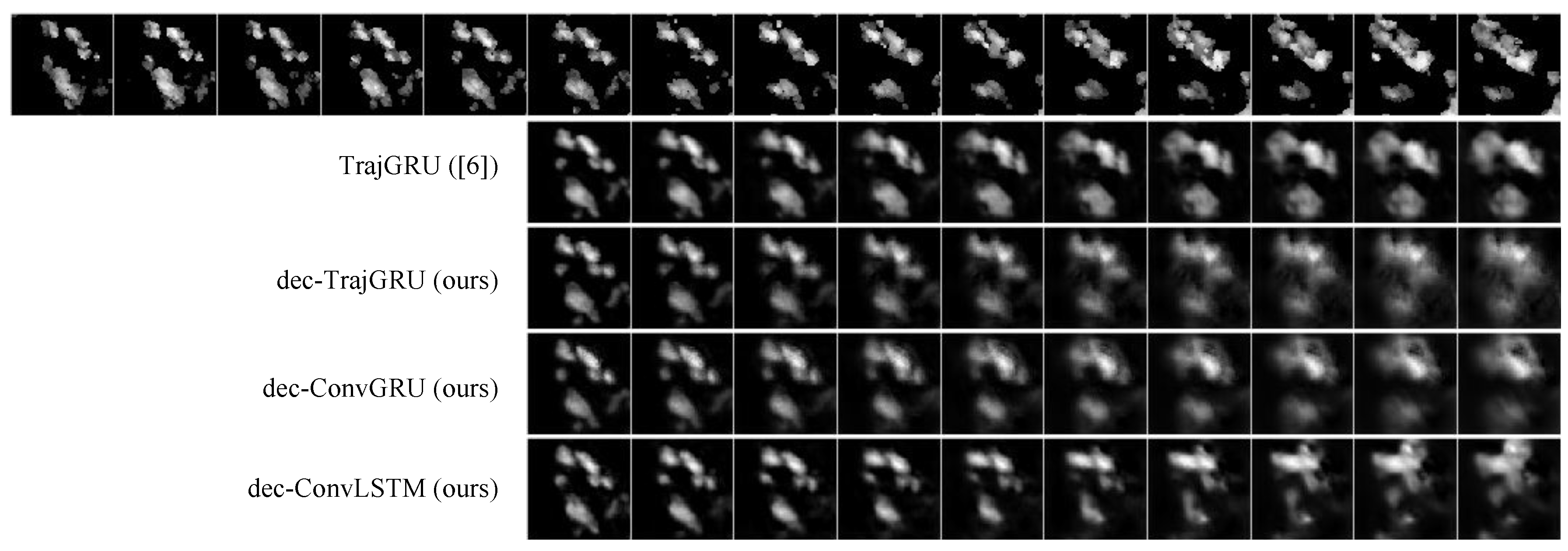
However, we also observed the trade-off between the ability to estimate stronger changes of precipitation particles with the ability to generate sharp images. Intuitively, the dec-TrajGRU model produced more reasonable images than the others, but it also suffered more from the blurry effect (see Figure 7). This can be explained by the fact that, in the context of high uncertainty, the top layers were not affected much by the patterns seen before and produced a reasonable abstract estimation of the overview of the image (presented as the cells’ outputted feature maps). These estimated feature maps are then upsampled and used to guide the lowest layer to estimate small local patches. The blurry effect appears mainly in these upsamling operations (because of having less detail information than the previous models), and is not solved well by the local estimating operations, as these operations are guided by MSE, a global-evaluating loss function. That was why we believed that adding other local-orienting loss functions can be a supplementary solution.
4.3. Evaluation of IQA-Based Loss Functions
In this experiment, we illustrated the effectiveness of several combined loss functions on the dec-TrajGRU model in Section 4.2. Firstly, we used the previous training settings and observed that using only MAE, SSIM or MS-SSIM as the loss function would significantly hurt the MSE-test performance, even though the overall performance could be slightly improved. This might lead to a poor estimation of the global changes in predicted images. Therefore, we focused on combining MSE with others to find the reasonably best function. To balance the magnitude of MSE and other measures in combined loss functions, we set , . Moreover, we also found that simply applying the previous early stopping technique on combined loss functions was not a good choice, because while some testing IQA metrics can be significantly improved, the MSE measure can be worsened. To deal with this issue, we trained the model with a combined loss function until the validating MSE got to an equal to or lower than the validation error in Section 4.2 (which was ). Then, the early stopping technique was used to terminate the training process. This strategy is simple but very important and effective to keep reasonable testing MSE.
Table 3 shows the testing results of three single-measure loss functions and the most effective combined ones (some other combinations such as SSIM + MS-SSIM did not provide interesting results). It is clear that using single-measure functions would increase the testing result of that measure, but decrease the testing-MSE significantly. In general, the combinations with the presence of SSIM seemed to be better than others, and the best loss function in this context is MSE + MAE + SSIM. To our surprise, it even improved on testing-MSE and testing-MS-SSIM over the model trained with only MSE or MS-SSIM. Comparing to the three models following Shi et al. [6], our best MSE measure was better. Moreover, using only SSIM or MAE + SSIM also enhanced MAE and MS-SSIM significantly. As argued in Section 4.2, our network tends to make strong assumptions about the global change rather than the local correlations, adding metrics which focus on local properties such as SSIM is a helpful compensation. Since it was able to produce more accurate predictions, other testing metrics could be improved too.
From the above results, we were able to confirm that using some common IQA metrics (and MAE) to train neural networks can produce less blurry images in the REE tasks than using only MSE. However, MSE still plays an important role to provide information about the global assumption. We illustrate these findings by the example in Figure 8. It is also important to note that the calculation of these IQA metrics did not significantly increase the training time, thanks to the very fast GPU-based execution of TensorFlow. This means that using IQA metrics for training neural networks in the REE tasks is a very cheap but effective solution, not only for our proposed structure but any other network architectures. In addition, we also found that using MS-SSIM seemed to be ineffective. The main reason can be because MS-SSIM is a multi-scale estimation technique, which is similar to the network structure and hence can not compensate its weakness. This result is opposite to the conclusion in [25] (about static image generation tasks). Using MAE only also seemed to be a poor choice. This means that the behaviors of IQA metrics can be different when being brought from CV tasks to the REE tasks, or more general the image processing applications in remote sensing.
To further confirm the meanings of our study findings in a closer view to an operational context, we compared the three best models in this part (chosen based-on the Overall Improvement) with the considered best one in [6] (TrajGRU in Section 4.1) in terms of Critical Success Index (CSI), False Alarm Rate (FAR), and Probability Of Detection (POD) metrics. We assumed that the dBZ values could be calculated by . With this conversion, the dBZ range in the test set is , and the proportions of dBZ thresholds 5, 20 and 40 are about , and , respectively. Table 4 provides an overall comparison over CSI, FAR and POD of these thresholds. While our model trained with MSE + SSIM was better than the previous best in seven among nine criteria, the two remaining models significantly outperformed that baseline in all criteria. Especially with heavier events, our models showed better overall predictions. We also tried other gains and offsets for the conversion and saw similar results. Hence, it can be concluded that the improvements in image quality are helpful for serving common operational expectations.
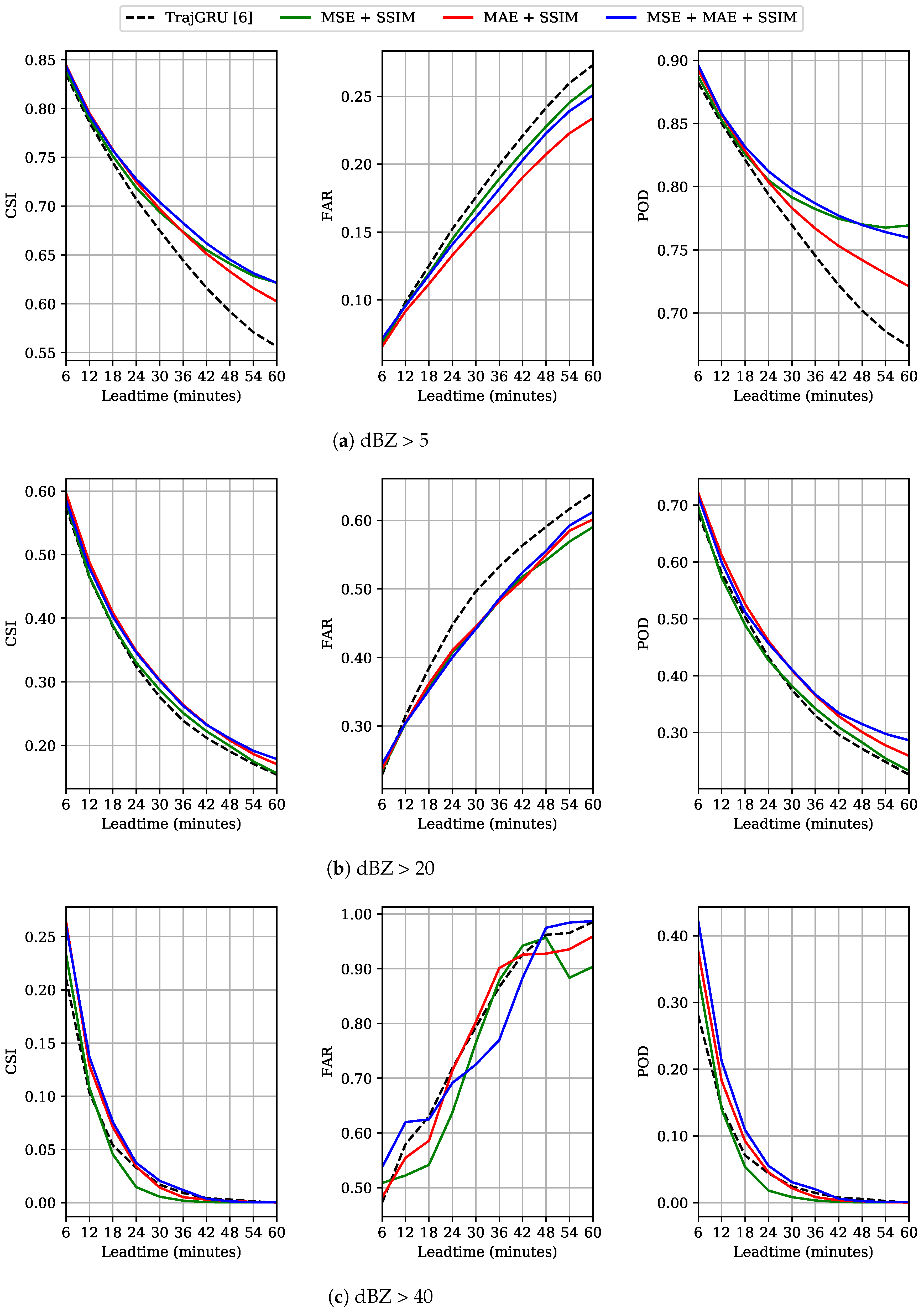
However, we realized that the models could work well with the dBZ thresholds 5 and 20 but were not stable with the dBZ threshold 40 (very low CSI but very high FAR). To analyze this issue more clearly, we plotted the frame-wise scores of these measures in Figure 9. In the cases of dBZ > 5 and dBZ > 20, all models performed similarly for the first several steps, but our models were more accurate with the remaining ones. In the case of dBZ > 40, our models were often better for several starting steps (except for the MSE + SSIM model), but the quality of all models degraded rapidly, with the CSI and POD scores becoming nearly zero after 42 min. We argued that there could be several reasons. Firstly, the train and test data have high uncertainty and heavy rain rarely occurs (0.35%). As can be inferred from the results in Figure 3, these events can be considered as outliers and are extremely difficult to model. This also made the evaluation vulnerable to noises (there are a number of white dots in the images, meaning very high rain-rate). Secondly, DL methods usually need big amount of data but the employed dataset is still considerably small in a DL context. The task is also more challenging with the test-size equals a half of the training-size. Thirdly, as limited by the fixed sequence length, we set a short input sequence and the models did not have enough information about the intensity change to estimate it well. Finally, our approach was driven to cope with the general precipitation rather than to focus on heavy rain. We believed that this issue can be solved by assigning higher weights on high rain rates (as in [6]), and using a bigger dataset with longer input sequences.
Interestingly, Figure 9c shows that the (MSE + SSIM) model degraded more rapidly than the others in terms of CSI and POD, but made the least wrong predictions in terms of FAR. We argued that using MSE for our models led to the fact that they did not make strong assumptions about the change of high intensity, and adding MAE was helpful. This argument agrees with the finding in [6], i.e. using MAE is helpful for predicting heavier rain. This can be because MSE squares the distance between two values, and in the intensity range , an error evaluation might become less and less important. On the other hand, MAE keeps the original distance of intensity to guide the training process. Because DL models usually produce low values in the initial training steps, and need the guidance from the loss functions to increase them, MAE could do better than MSE in this case. Moreover, SSIM might estimate the intensity well, but locally, and could not compensate MSE well enough. It should be noted that the FAR score of the MSE + SSIM model might fluctuate, as in Figure 9c, because there are some high intensity particles suddenly appeared and decreased in some samples. However, we thought that it was hard to draw an adequate conclusion for this outlier case, and suggested this issue for the future work.
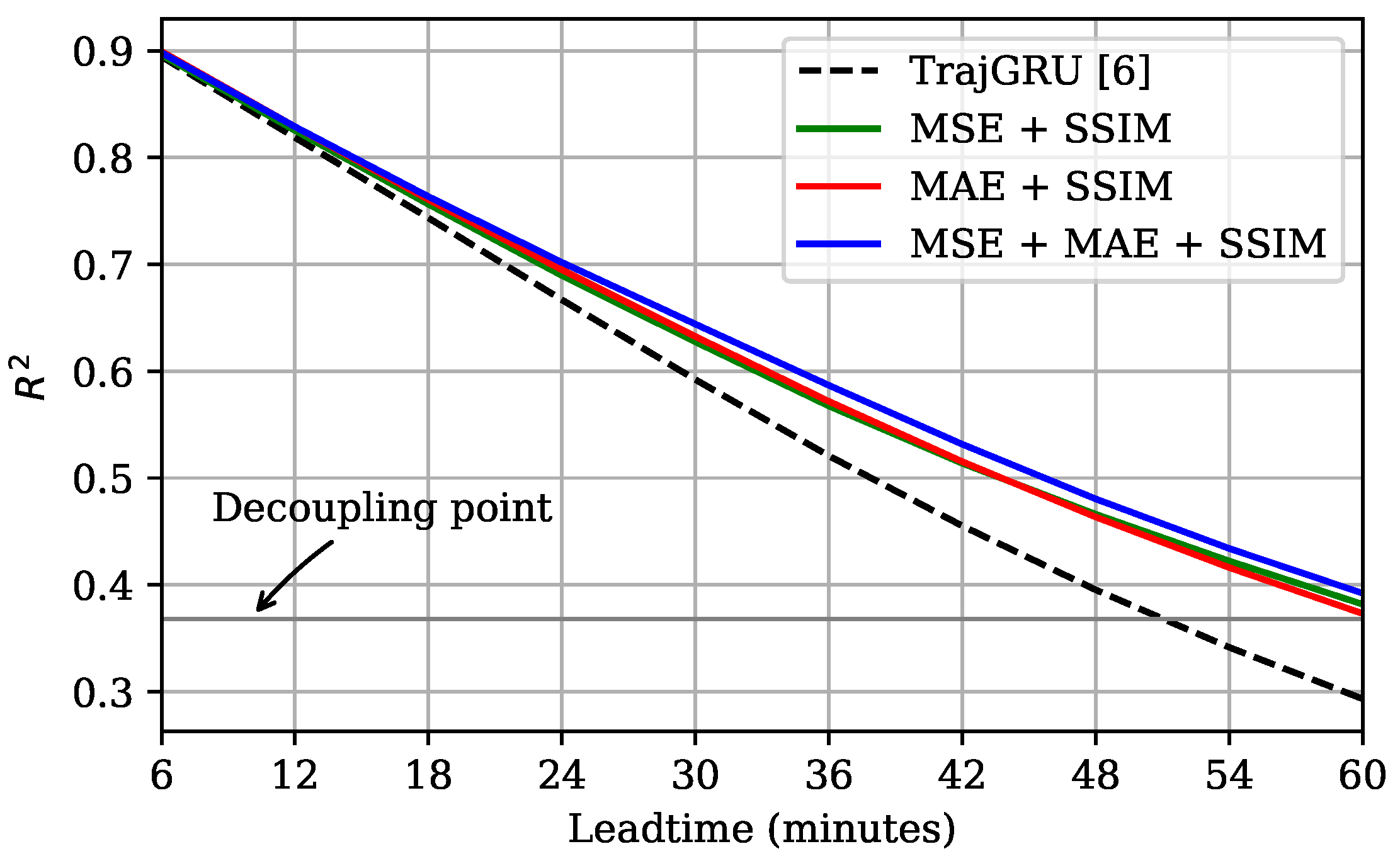
In general, we argued that the MSE + SSIM was still competitive with the MAE + SSIM and MSE + MAE + SSIM models, and outperformed the TrajGRU model. This is strongly supported by the evidence in Figure 10, which shows that the coefficient of determination of our three models did not fall below the decoupling point in all 10 steps, but the TrajGRU model failed after Step 8 (48 min).
5. Conclusions and Future Work
We have presented a different viewpoint from traditional approaches on some ConvRNNs methods for the REE task. Using the Shenzhen data, which poses a difficult context for nowcasting models, we demonstrated that the popular MSE loss function can mislead the evaluation of models. To cope with the challenge of the dataset, we then proposed a new sequence-to-sequence structure by reducing the number of channels of recurrent layers through bottom-to-top. Experimental results show that dec-seq2seq models were more tolerant to the high and increasing uncertainty in the data. Even though our design is specific-case driven, it is reasonable because it is based on a realistic situation. In the context of climate change, such situation is more likely to occur than the common assumption of i.i.d distribution in the machine learning literature. We confirmed this experimental finding on the MovingMNIST++ data by generating test sets with significantly different characteristics from the training set. We further improved the prediction quality of the REE task by using two popular IQA metrics, SSIM and MS-SSIM, to form combined loss functions. To the best of our knowledge, this is the first use of IQA metrics for training neural networks in the REE task and successfully produced less blurry images. Our experimental findings show that this approach can be a cheap solution but very effective for guiding RNNs in remote sensing areas. In more detail, we found that SSIM is a strong candidate for the REE task, and using SSIM to combine with MSE and MAE was the best loss function. Finally, we concluded that improving predicted images in terms of CV standards can lead to improved CSI, FAR and POD measures.
For the future work, we propose applying the viewpoint in this study for the multi-channel REE task, which needs to forecast different radar images at different elevation angles, larger spatial and temporal scales, and finer resolutions (such as NEXRAD data). We also believe that the prediction quality can be enhanced more by blending IQA metrics with the GAN-loss, as well as incorporating the training loss at the abstract levels. Particularly, an investigation of these techniques for heavy rain will be highly meaningful.
Author Contributions
Q.-K.T. collected the data, developed the model, and designed and performed the experiments. Q.-K.T. and S.-K.S. analyzed the results. Q.-K.T. wrote the paper. S.-K.S. provided the overall guidance to the study, and reviewed and edited the manuscript.
Funding
Construction of Research Data Open Platform and its Utilization Support (Project No.: K-19-L01-C04).
Acknowledgments
This work formed part of research project carried out at the Korea Institute of Science and Technology Information (KISTI). We thank Dr. Jung-Ho Uhm, Dr. Seongchan Kim and Ph.D candidate Seungkyun Hong in KISTI for their great supports and discussions. Finally, we thank the organizers of CIKM AnalytiCup 2017 for sharing their data freely.
Conflicts of Interest
The authors declare no conflict of interest.
Appendix A. Network Sizes and Training Costs

Table A1.
Network sizes and training costs of the models adapted from [6] (the top three rows) and our proposed dec-seq2seq models (the bottom three rows). Because of the early stopping technique, models might terminate after different numbers of iterations, hence we reported the average time of one iteration here.
| No. of Trainable Variables | No. of Trainable Parameters | Highest GPU Consumption (MB) | One Iteration (minutes) | |
|---|---|---|---|---|
| TrajGRU [6] | 115 | 4,341,677 | 9159 | 1.8 |
| ConvGRU [6] | 81 | 4,555,265 | 4551 | 1.5 |
| ConvLSTM [6] | 121 | 7,463,009 | 4551 | 2.1 |
| dec-TrajGRU | 113 | 1,276,669 | 4807 | 1.7 |
| dec-ConvGRU | 79 | 1,066,081 | 1479 | 1.1 |
| dec-ConvLSTM | 119 | 2,544,609 | 1479 | 1.5 |
Appendix B. Evaluation of TrajGRU and dec-TrajGRU models on MovingMNIST++
To demonstrate our experimental findings in the context of Shenzhen data, we tried to simulate its properties by an experiment on the MovingMNIST++ data with one training set and several test sets. In this experiment, the length of both the input and output sequences was 10, and the image size was pixels. We generated the training set (8000 samples for training and 2000 samples for validating) with two randomly selected digits among the first 40,000 images in the MNIST dataset, following the implementation in [6]. To form different test sets (each had 4000 samples) with high and different levels of uncertainty, we randomly chose one, two or three digits among the remaining 10,000 images, and gradually changed the generating settings. This is similar to the out-of-domain testing in [5], where the images in the test sets did not appear in the training set. Since we tried to simulate the situation of weather data, our test data were even more uncertain. The generating settings are given in Table A2. The testing results given in Table A3 show that our dec-TrajGRU model seemed to be less mistaken than TrajGRU when the uncertainty changed, especially when the scaling variation is higher. Figure A1 illustrates this argument intuitively, in which both models made wrong assumption.
Table A2.
Generating settings of the training set and three test sets with different levels of uncertainty. To vary the intensity of images after generating each sample, we randomly generated an integer between max_range and scale the whole sequence to that number.
Table A2.
Generating settings of the training set and three test sets with different levels of uncertainty. To vary the intensity of images after generating each sample, we randomly generated an integer between max_range and scale the whole sequence to that number.
| Variables | Training Set | Test Set 1 | Test Set 2 | Test Set 3 | Test Set 4 |
|---|---|---|---|---|---|
| max_velocity_scale | 3.6 | 4.6 | 5.6 | 5.6 | 4.6 |
| initial_velocity_range | [0.0, 3.6] | [0.0, 4.6] | [2.0, 5.6] | [0.0, 5.6] | [2.0, 4.6] |
| scale_variation_range | [0.9, 1.1] | [0.8, 1.2] | [0.7, 1.3] | [0.6, 1.4] | [0.5, 1.5] |
| rotation_angle_range | [−30, 30] | [−45, 45] | [−45, 45] | [−45, 45] | [−40, 40] |
| global_rotation_angle_range | [−20, 20] | [−45, 45] | [−30, 30] | [−45, 45] | [−30, 30] |
| illumination_factor_range | [0.6, 1.0] | [0.8, 1.2] | [0.7, 1.3] | [0.8, 1.2] | [0.8, 1.2] |
| max_range | [100, 200] | [80, 220] | [80, 220] | [80, 220] | [80, 220] |
Table A3.
Validating and testing MSE × 100 of TrajGRU and dec-TrajGRU models.
| Validating | Test Set 1 | Test Set 2 | Test Set 3 | Test Set 4 | |
|---|---|---|---|---|---|
| TrajGRU [6] | 0.6833 | 0.9135 | 0.8342 | 1.1543 | 1.2179 |
| dec-TrajGRU (ours) | 0.7296 | 0.9114 | 0.8246 | 1.1420 | 1.1825 |
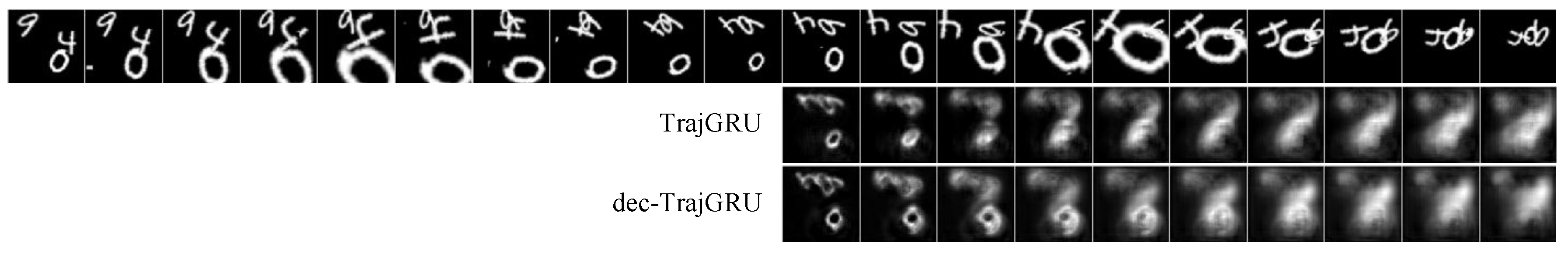
Figure A1.
Example of MovingMNIST++ prediction (Test set 4). We observed that dec-TrajGRU often made less wrong assumption when going further into the future.
Figure A1.
Example of MovingMNIST++ prediction (Test set 4). We observed that dec-TrajGRU often made less wrong assumption when going further into the future.

References
- Wang, C.; Hong, Y. Application of Spatiotemporal Predictive Learning in Precipitation Nowcasting. In Proceedings of the American Geophysical Union, Fall Meeting 2018, Washingtong, DC, USA, 10–14 December 2018. [Google Scholar]
- Heye, A.; Venkatesan, K.; Cain, J. Precipitation Nowcasting: Leveraging Deep Recurrent Convolutional Neural Networks. In Proceedings of the Cray User Group (CUG) 2017–Caffeinated Computing, Redmond, WA, USA, 8–11 May 2017. [Google Scholar]
- Yu, W.; Nakakita, E.; Kim, S.; Yamaguchi, K. Improvement of rainfall and flood forecasts by blending ensemble NWP rainfall with radar prediction considering orographic rainfall. J. Hydrol. 2015, 531, 494–507. [Google Scholar] [CrossRef]
- Li, L.; He, Z.; Chen, S.; Mai, X.; Zhang, A.; Hu, B.; Li, Z.; Tong, X. Subpixel-Based Precipitation Nowcasting with the Pyramid Lucas–Kanade Optical Flow Technique. Atmosphere 2018, 9, 260. [Google Scholar] [CrossRef]
- Shi, X.; Chen, Z.; Wang, H.; Yeung, D.Y.; Wong, W.K.; Woo, W.c. Convolutional LSTM network: A machine learning approach for precipitation nowcasting. In Proceedings of the Advances in Neural Information Processing Systems (NIPS), Montreal, QC, Canada, 7–12 December 2015; pp. 802–810. [Google Scholar]
- Shi, X.; Gao, Z.; Lausen, L.; Wang, H.; Yeung, D.Y.; Wong, W.K.; Woo, W.C. Deep Learning for Precipitation Nowcasting: A Benchmark and a New Model. In Proceedings of the Advances in Neural Information Processing Systems (NIPS), Montreal, QC, Canada, 7–12 December 2015; pp. 5617–5627. [Google Scholar]
- Shi, E.; Li, Q.; Gu, D.; Zhao, Z. A Method of Weather Radar Echo Extrapolation Based on Convolutional Neural Networks. In Proceedings of the International Conference on Multimedia Modeling (MMM 2018), Bangkok, Thailand, 5–7 February 2018; Springer: Cham, Switzerland, 2018; Volume 10704, pp. 16–28. [Google Scholar] [CrossRef]
- Yao, Y.; Li, Z. CIKM AnalytiCup 2017: Short-Term Precipitation Forecasting Based on Radar Reflectivity Images. In Proceedings of the Conference on Information and Knowledge Management, Short-Term Quantitative Precipitation Forecasting Challenge, Singapore, 6–10 November 2017. [Google Scholar]
- Asanjan, A.A.; Yang, T.; Hsu, K.; Sorooshian, S.; Lin, J.; Peng, Q. Short-term Precipitation Forecast based on the PERSIANN system and the Long ShortTerm Memory (LSTM) Deep Learning Algorithm. J. Geophys. Res. Atmos. 2018, 123, 12543–12563. [Google Scholar] [CrossRef]
- Ballas, N.; Yao, L.; Pal, C.; Courville, A. Delving deeper into convolutional networks for learning video representations. In Proceedings of the International Conference on Learning Representations (ICLR), San Juan, Puerto Rico, 2–4 May 2016. [Google Scholar]
- Germann, U.; Zawadzki, I. Scale-dependence of the predictability of precipitation from continental radar images. Part I: Description of the methodology. Mon. Weather Rev. 2002, 130, 2859–2873. [Google Scholar] [CrossRef]
- Germann, U.; Zawadzki, I. Scale dependence of the predictability of precipitation from continental radar images. Part II: Probability forecasts. J. Appl. Meteorol. 2004, 43, 74–89. [Google Scholar] [CrossRef]
- Turner, B.; Zawadzki, I.; Germann, U. Predictability of precipitation from continental radar images. Part III: Operational nowcasting implementation (MAPLE). J. Appl. Meteorol. 2004, 43, 231–248. [Google Scholar] [CrossRef]
- Lee, H.C.; Lee, Y.H.; Ha, J.C.; Chang, D.E.; Bellon, A.; Zawadzki, I.; Lee, G. McGill Algorithm for Precipitation Nowcasting by Lagrangian Extrapolation (MAPLE) applied to the South Korean radar network. Part II: Real-time verification for the summer season. Asia-Pac. J. Atmos. Sci. 2010, 46, 383–391. [Google Scholar] [CrossRef]
- Tang, J.; Matyas, C. A Nowcasting Model for Tropical Cyclone Precipitation Regions Based on the TREC Motion Vector Retrieval with a Semi-Lagrangian Scheme for Doppler Weather Radar. Atmosphere 2018, 9, 200. [Google Scholar] [CrossRef]
- Sato, R.; Kashima, H.; Yamamoto, T. Short-Term Precipitation Prediction with Skip-Connected PredNet. In Proceedings of the ICANN 2018: 27th International Conference on Artificial Neural Networks, Rhodes, Greece, 4–7 October 2018; Kůrková, V., Manolopoulos, Y., Hammer, B., Iliadis, L., Maglogiannis, I., Eds.; Lecture Notes in Computer Science. Springer: Cham, Switzerland, 2018; Volume 11141, pp. 373–382. [Google Scholar] [CrossRef]
- Klein, B.; Wolf, L.; Afek, Y. A dynamic convolutional layer for short range weather prediction. In Proceedings of the IEEE Conference on Computer Vision and Pattern Recognition, Boston, MA, USA, 7–12 June 2015; pp. 4840–4848. [Google Scholar]
- Tran, D.; Bourdev, L.; Fergus, R.; Torresani, L.; Paluri, M. Learning spatiotemporal features with 3d convolutional networks. In Proceedings of the IEEE International Conference on Computer Vision (ICCV), Washington, DC, USA, 7–13 December 2015; pp. 4489–4497. [Google Scholar]
- Woo, W.C.; Wong, W.K. Operational Application of Optical Flow Techniques to Radar-Based Rainfall Nowcasting. Atmosphere 2017, 8, 48. [Google Scholar] [CrossRef]
- Kalchbrenner, N.; Oord, A.v.d.; Simonyan, K.; Danihelka, I.; Vinyals, O.; Graves, A.; Kavukcuoglu, K. Video pixel networks. In Proceedings of the 34th International Conference on Machine Learning (ICML), Sydney, Australia, 6–11 August 2017. [Google Scholar]
- Villegas, R.; Yang, J.; Zou, Y.; Sohn, S.; Lin, X.; Lee, H. Learning to generate long-term future via hierarchical prediction. In Proceedings of the 34th International Conference on Machine Learning (ICML), Sydney, Australia, 6–11 August 2017. [Google Scholar]
- Luo, W.; Liu, W.; Gao, S. Remembering history with convolutional lstm for anomaly detection. In Proceedings of the 2017 IEEE International Conference on Multimedia and Expo (ICME), Hong Kong, China, 10–14 July 2017; pp. 439–444. [Google Scholar]
- Singh, S.; Sarkar, S.; Mitra, P. A deep learning based approach with adversarial regularization for Doppler weather radar ECHO prediction. In Proceedings of the 2017 IEEE Geoscience and Remote Sensing Symposium (IGARSS), Fort Worth, TX, USA, 23–28 July 2017; pp. 5205–5208. [Google Scholar]
- Kim, S.; Kim, H.; Lee, J.; Yoon, S.; Kahou, S.E.; Kashinath, K.; Prabhat, M. Deep-Hurricane-Tracker: Tracking and Forecasting Extreme Climate Events; Technical Report; Lawrence Livermore National Lab. (LLNL): Livermore, CA, USA, 2018. [Google Scholar]
- Zhao, H.; Gallo, O.; Frosio, I.; Kautz, J. Loss functions for image restoration with neural networks. IEEE Trans. Comput. Imaging 2017, 3, 47–57. [Google Scholar] [CrossRef]
- Mathieu, M.; Couprie, C.; LeCun, Y. Deep multi-scale video prediction beyond mean square error. In Proceedings of the International Conference on Learning Representations (ICLR), San Juan, Puerto Rico, 2–4 May 2016. [Google Scholar]
- Palubinskas, G. Image similarity/distance measures: What is really behind MSE and SSIM? Int. J. Image Data Fusion 2017, 8, 32–53. [Google Scholar] [CrossRef]
- Xia, Y.; Chen, Z. Quality assessment for remote sensing images: Approaches and applications. In Proceedings of the 2015 IEEE International Conference on Systems, Man, and Cybernetics (SMC), Kowloon, China, 9–12 October 2015; pp. 1029–1034. [Google Scholar]
- Yang, J.; Zhao, Y.; Yi, C.; Chan, J.C.W. No-reference hyperspectral image quality assessment via quality-sensitive features learning. Remote Sens. 2017, 9, 305. [Google Scholar] [CrossRef]
- Dosovitskiy, A.; Brox, T. Generating images with perceptual similarity metrics based on deep networks. In Proceedings of the Advances in Neural Information Processing Systems (NIPS), Barcelona, Spain, 5–10 December 2016; pp. 658–666. [Google Scholar]
- Lu, C.; Hirsch, M.; Schölkopf, B. Flexible spatio-temporal networks for video prediction. In Proceedings of the IEEE Conference on Computer Vision and Pattern Recognition, Honolulu, HI, USA, 21–26 July 2017; pp. 6523–6531. [Google Scholar]
- Lee, A.X.; Zhang, R.; Ebert, F.; Abbeel, P.; Finn, C.; Levine, S. Stochastic Adversarial Video Prediction. arXiv 2018, arXiv:1804.01523. [Google Scholar]
- Simonyan, K.; Zisserman, A. Very deep convolutional networks for large-scale image recognition. In Proceedings of the International Conference on Learning Representations (ICLR), San Diego, CA, USA, 7–9 May 2015. [Google Scholar]
- CIKM AnalytiCup 2017 Dataset. Available online: https://tianchi.aliyun.com/dataset/dataDetail?dataId=1085 (accessed on 30 April 2019).
- Wang, Z.; Simoncelli, E.P.; Bovik, A.C. Multiscale structural similarity for image quality assessment. In Proceedings of the Thrity-Seventh Asilomar Conference on Signals, Systems & Computers, Pacific Grove, CA, USA, 9–12 November 2003; Volume 2, pp. 1398–1402. [Google Scholar]
- Wang, Z.; Bovik, A.C.; Sheikh, H.R.; Simoncelli, E.P. Image quality assessment: From error visibility to structural similarity. IEEE Trans. Image Process. 2004, 13, 600–612. [Google Scholar] [CrossRef] [PubMed]
- Wang, Z.; Bovik, A.C. Mean squared error: Love it or leave it? A new look at signal fidelity measures. IEEE Signal Process. Mag. 2009, 26, 98–117. [Google Scholar] [CrossRef]
- Inamdar, D.; Leblanc, G.; Soffer, R.J.; Kalacska, M. The Correlation Coefficient as a Simple Tool for the Localization of Errors in Spectroscopic Imaging Data. Remote Sens. 2018, 10, 231. [Google Scholar] [CrossRef]
- Finn, C.; Goodfellow, I.; Levine, S. Unsupervised learning for physical interaction through video prediction. In Proceedings of the Advances in Neural Information Processing Systems (NIPS), Barcelona, Spain, 5–10 December 2016; pp. 64–72. [Google Scholar]
Figure 1.
Vanilla sequence-to-sequence structure with two stacked layers for constructing RNN models in precipitation nowcasting (adapted from [6]). This design consists of an encoder (white) and a decoder (gray). The circles are RNNs cells and the solid arrows are the cells’ input and output, while the dotted arrows are recurrent operations. In the encoder, the outputs are downsampled by convolutional operations, while, in the decoder, they are upsampled by deconvolutional operations. Thanks to that, models can predict at different spatial scales.

Figure 2.
The trajectory generation network in a TrajGRU cell for tracking a subset of points between two steps (drawn from the implementation of Shi et al. [6]). The dotted arrows denote the convolution operations, where m is the cell’s state size, c is the cell’s number of channels, k is the convolution kernel size, s is the convolution stride size, and L is the number of neighboring points. In [6], the number of channels of the feature maps for fusing the two steps is fixed at 32. The output of this block has channels since it needs to estimate both the horizontal and vertical movements of each point.

Figure 3.
Histograms of the dataset divided into three parts (best viewed in color). For convenient comparison and presentation, we scaled the distribution of each set to the range [0, 1] and drew its histogram as a line. Note that the zero values were excluded as they dominate the data space.
Figure 3.
Histograms of the dataset divided into three parts (best viewed in color). For convenient comparison and presentation, we scaled the distribution of each set to the range [0, 1] and drew its histogram as a line. Note that the zero values were excluded as they dominate the data space.

Figure 4.
The three-layer TrajGRU model for one-channel image sequence (two input steps and two output steps). The cells are presented in rectangles with state ( is the size of image, feature map, or cell states, and b is the number of feature maps or state maps). One down-sampling is a convolution, and one up-sampling is a deconvolution. In each layer, the step-to-step transition is done by a “trajectory-net” (Figure 2), which produces flow fields used for a warping process to calculate the current state. In this figure, L is the number of tracked points, while k is the kernel size and c is the number of filters of the convolutional operations. ConvGRU or ConvLSTM models can be implemented by simply replacing these trajectory-net blocks with the common convolution with the stride size . In this study, we used kernel size for all of the step-to-step transitions.

Figure 5.
Example of predicted results of three models following Shi et al. [6]. In the the first row, the five left-most images are the input and then ten right-most images are the expected output. Predicted images of three models are drawn in the second through the fourth rows.
Figure 5.
Example of predicted results of three models following Shi et al. [6]. In the the first row, the five left-most images are the input and then ten right-most images are the expected output. Predicted images of three models are drawn in the second through the fourth rows.

Figure 6.
Comparison of our models with the models following Shi et al. [6] in terms of lead-time error (MSE) on the test set. Best view in color.
Figure 6.
Comparison of our models with the models following Shi et al. [6] in terms of lead-time error (MSE) on the test set. Best view in color.

Figure 7.
Example of predicted results of three dec-seq2seq models. The result of TrajGRU from Section 4.1 is copied here for convenient comparison.
Figure 7.
Example of predicted results of three dec-seq2seq models. The result of TrajGRU from Section 4.1 is copied here for convenient comparison.

Figure 8.
Example of predicted results of the dec-TrajGRU model trained with different loss functions. The result of dec-TrajGRU from Section 4.2 is copied here for convenient comparing.
Figure 8.
Example of predicted results of the dec-TrajGRU model trained with different loss functions. The result of dec-TrajGRU from Section 4.2 is copied here for convenient comparing.

Figure 9.
Frame-wise CSI, FAR and POD scores of of predicting rainfall situations at different dBZ thresholds. Best view in color.
Figure 9.
Frame-wise CSI, FAR and POD scores of of predicting rainfall situations at different dBZ thresholds. Best view in color.

Figure 10.
Coefficients of determination over lead times. Value of the decoupling point is . Best view in color.
Figure 10.
Coefficients of determination over lead times. Value of the decoupling point is . Best view in color.

Table 1.
Performances of models following Shi et al. [6] (Figure 4). For convenient presentation, we scaled up MSE 100 times and MAE 10 times. MSE and MAE are expected to be decreased, while SSIM, MS-SSIM and PCC are expected to be increased. The best value in each column is presented in bold-face.
| Validating | Testing | |||||
|---|---|---|---|---|---|---|
| Best MSE | MSE | MAE | SSIM | MS-SSIM | PCC | |
| Last input | - | 1.6804 | 0.8120 | 0.4552 | 0.4207 | 0.6234 |
| TrajGRU ([6]) | 0.4455 | 0.9950 | 0.6599 | 0.4920 | 0.5564 | 0.7450 |
| ConvGRU ([6]) | 0.3143 | 0.9998 | 0.6408 | 0.5380 | 0.5621 | 0.7507 |
| ConvLSTM ([6]) | 0.3165 | 0.9962 | 0.6463 | 0.5280 | 0.5629 | 0.7501 |
Table 2.
Performances of three dec-seq2seq models. The presentation is similar to Table 1.
Table 2.
Performances of three dec-seq2seq models. The presentation is similar to Table 1.
| Validating | Testing | |||||
|---|---|---|---|---|---|---|
| Best MSE | MSE | MAE | SSIM | MS-SSIM | PCC | |
| dec-TrajGRU | 0.7003 | 0.8892 | 0.6401 | 0.4981 | 0.5742 | 0.7718 |
| dec-ConvGRU | 0.5793 | 0.8992 | 0.6444 | 0.4830 | 0.5789 | 0.7699 |
| dec-ConvLSTM | 0.4887 | 0.9524 | 0.6476 | 0.4987 | 0.5783 | 0.7593 |
Table 3.
Testing performances of the dec-TrajGRU model trained with different loss functions. For convenience, we used the “+” sign to denote the combination. The overall improvement is the averaged percentage of advantages in the synthetic comparison with the dec-TrajGRU model trained with only MSE in Section 4.2.
| Testing | Overall Improvement | |||||
|---|---|---|---|---|---|---|
| MSE | MAE | SSIM | MS-SSIM | PCC | ||
| MAE | 0.9536 | 0.6031 | 0.5673 | 0.5773 | 0.7671 | 2.30% |
| SSIM | 0.9651 | 0.5880 | 0.5934 | 0.5927 | 0.7692 | 4.16% |
| MS-SSIM | 0.9632 | 0.6384 | 0.5325 | 0.5865 | 0.7668 | -0.10% |
| MSE + MAE | 0.8865 | 0.6132 | 0.5346 | 0.5907 | 0.7776 | 2.93% |
| MSE + SSIM | 0.8870 | 0.5994 | 0.5762 | 0.5927 | 0.7768 | 5.07% |
| MSE + MS-SSIM | 0.8991 | 0.6348 | 0.4997 | 0.5849 | 0.7719 | 0.23% |
| MAE + SSIM | 0.9255 | 0.5787 | 0.5924 | 0.5957 | 0.7770 | 5.61% |
| MAE + MS-SSIM | 0.9322 | 0.6001 | 0.5689 | 0.5931 | 0.7738 | 3.67% |
| MSE + MAE + SSIM | 0.8743 | 0.5836 | 0.5829 | 0.5994 | 0.7845 | 6.56% |
| MSE + MAE + MS-SSIM | 0.8941 | 0.6177 | 0.5424 | 0.5846 | 0.7720 | 2.58% |
Table 4.
Comparison of our three best models with TrajGRU [6] implemented in Section 4.1 over CSI, FAR and POD (average score of the whole sequence). CSI and POD are expected to increase while FAR is expected to decrease.
Table 4.
Comparison of our three best models with TrajGRU [6] implemented in Section 4.1 over CSI, FAR and POD (average score of the whole sequence). CSI and POD are expected to increase while FAR is expected to decrease.
| CSI | FAR | POD | |||||||
|---|---|---|---|---|---|---|---|---|---|
| dBZ Threshold | 5 | 20 | 40 | 5 | 20 | 40 | 5 | 20 | 40 |
| TrajGRU [6] | 0.6729 | 0.2994 | 0.0436 | 0.1812 | 0.4815 | 0.7900 | 0.7646 | 0.3949 | 0.0593 |
| MSE + SSIM | 0.7013 | 0.3059 | 0.0411 | 0.1726 | 0.4443 | 0.7539 | 0.8027 | 0.3991 | 0.0568 |
| MAE + SSIM | 0.6996 | 0.3208 | 0.0524 | 0.1579 | 0.4490 | 0.7788 | 0.7879 | 0.4264 | 0.0734 |
| MSE + MAE + SSIM | 0.7069 | 0.3192 | 0.0549 | 0.1683 | 0.4513 | 0.7797 | 0.8053 | 0.4296 | 0.0859 |
© 2019 by the authors. Licensee MDPI, Basel, Switzerland. This article is an open access article distributed under the terms and conditions of the Creative Commons Attribution (CC BY) license (http://creativecommons.org/licenses/by/4.0/).
Share and Cite
MDPI and ACS Style
Tran, Q.-K.; Song, S.-k. Computer Vision in Precipitation Nowcasting: Applying Image Quality Assessment Metrics for Training Deep Neural Networks. Atmosphere 2019, 10, 244. https://doi.org/10.3390/atmos10050244
AMA Style
Tran Q-K, Song S-k. Computer Vision in Precipitation Nowcasting: Applying Image Quality Assessment Metrics for Training Deep Neural Networks. Atmosphere. 2019; 10(5):244. https://doi.org/10.3390/atmos10050244
Chicago/Turabian StyleTran, Quang-Khai, and Sa-kwang Song. 2019. "Computer Vision in Precipitation Nowcasting: Applying Image Quality Assessment Metrics for Training Deep Neural Networks" Atmosphere 10, no. 5: 244. https://doi.org/10.3390/atmos10050244
Note that from the first issue of 2016, this journal uses article numbers instead of page numbers. See further details here.