Considering Rain Gauge Uncertainty Using Kriging for Uncertain Data †
by
 , , and
Francesca Cecinati
1,* ,
,
Antonio M. Moreno-Ródenas
2,
Miguel A. Rico-Ramirez
1,
Marie-claire Ten Veldhuis
2 and
Jeroen G. Langeveld
2 1
Department of Civil Engineering, University of Bristol, Queen’s Building, University Walk, Bristol BS8 1TR, UK
2
Water Management Department, Technische Universiteit Delft, Building 23, Stevinweg 1, 2628 CN Delft, The Netherlands
*
Author to whom correspondence should be addressed.
†
A previous shorter version of the paper has been presented in the 10th World Congress of EWRA “Panta Rhei” Athens, Greece, 5–9 July 2017.
Atmosphere 2018, 9(11), 446; https://doi.org/10.3390/atmos9110446
Submission received: 8 August 2018
/
Revised: 1 November 2018
/
Accepted: 7 November 2018
/
Published: 14 November 2018
(This article belongs to the Special Issue Advances in Applications of Weather Radar Data)
Abstract
:In urban hydrological models, rainfall is the main input and one of the main sources of uncertainty. To reach sufficient spatial coverage and resolution, the integration of several rainfall data sources, including rain gauges and weather radars, is often necessary. The uncertainty associated with rain gauge measurements is dependent on rainfall intensity and on the characteristics of the devices. Common spatial interpolation methods do not account for rain gauge uncertainty variability. Kriging for Uncertain Data (KUD) allows the handling of the uncertainty of each rain gauge independently, modelling space- and time-variant errors. The applications of KUD to rain gauge interpolation and radar-gauge rainfall merging are studied and compared. First, the methodology is studied with synthetic experiments, to evaluate its performance varying rain gauge density, accuracy and rainfall field characteristics. Subsequently, the method is applied to a case study in the Dommel catchment, the Netherlands, where high-quality automatic gauges are complemented by lower-quality tipping-bucket gauges and radar composites. The case study and the synthetic experiments show that considering measurement uncertainty in rain gauge interpolation usually improves rainfall estimations, given a sufficient rain gauge density. Considering measurement uncertainty in radar-gauge merging consistently improved the estimates in the tested cases, thanks to the additional spatial information of radar rainfall data but should still be used cautiously for convective events and low-density rain gauge networks.
1. Introduction
Urban hydrology requires accurate rainfall data with high temporal and spatial resolutions [1]. Ideally the availability of very dense high-accuracy rain gauge networks could provide the necessary rainfall information but rarely national and regional networks meet the required gauge density and it is necessary to integrate the measurements with additional data [2]. Weather radars provide a full aerial coverage and commonly reach a 5-min temporal resolution and 1-km spatial resolution, sufficient for urban applications in medium-large urban areas but hardly offer the required accuracy [3,4]. It is recognised that merging radar rainfall data with rain gauge measurements allows to maintain the spatial coverage and resolution from radar and the accuracy of gauge measurements to improve the rainfall estimates [5,6,7]. One of the advantages of kriging-based merging methods is that the estimation of the kriging variance provides a starting point to estimate rainfall uncertainty. However, the standard kriging formulation allows to consider only a spatially uniform measurement uncertainty. In fact, the use of a nugget effect in the geostatistical model can represent measurement errors but does not allow to consider a different uncertainty for each measurement point [8,9]. In some applications, rain gauge uncertainty is assumed to be small enough to be neglected [10,11,12,13]. This can be done when the accumulation time is not too small [12] and when rain gauges are accurate and their data is correctly managed and calibrated [14,15,16,17]. Unfortunately, in many operational networks the importance of accurate rainfall data and of data quality control can be underestimated; budget and best practice knowledge can be limiting factors in a correct rain gauge network management. In these cases, the accuracy of rain gauges can drastically drop and the uncertainty associated with the measurements cannot be neglected anymore [18]. Additionally, frequently rain gauge networks are not dense enough to capture the spatial characteristics of rainfall in urban applications [19,20] and integrating different rain gauge networks, with different accuracy characteristics is often necessary.
The uncertainty in rain gauge rainfall data is due to different error sources [21]. Rain gauges are affected by predictable errors due, for example, to wind under-catch [15], losses due to wetting of rain gauge surfaces after a dry spell and losses due to evaporation [21]. For tipping-bucket devices, limits in the mechanical tipping at high intensities is an additional problem [17,22]. These errors can be modelled and partially corrected with calibration. Rain gauges are also affected by random errors, which cannot be predicted or deterministically modelled [23]. For example, partial or total blockage can occur due to leaves, snow (in absence of a heating system) and other materials transported by the wind (under regular maintenance, these effects should be limited in time), snow and hail melting or condensation can produce records even in the absence of precipitation, splashes and other water intrusions not related to precipitation can alter the records and animals or people can temporary interfere with the devices. For tipping-bucket rain gauges, additional random errors occur, like the partial filling of the bucket and delayed tipping at low intensities, the total or partial blockage of the tipping mechanism, or other mechanical problems. Another problem in the use of rain gauges as a ground reference is that they are representative of points, while they are often used as aerial reference, generating point-to-area errors [24,25,26,27]. In addition, poor data management can introduce additional errors, like missed recording of cleaning operations or maintenance, mismatch of temporal and spatial references, or absence of metadata on data calibration and processing, which introduce unknown errors. In this paper, a model is proposed to integrate measurement point errors in the rainfall uncertainty quantification.
The integration of point measurement uncertainty in kriging has been studied in literature. A solution in case of homoscedasticity is the use of the nugget effect [8,9] but it assumes that all rain gauge measurements are characterised by the same error. De Marsily [28] formulated a method to handle different variances for different point measurement errors, called Kriging for Uncertain Data (KUD). The formulation was further developed by Mazzetti and Todini [29].
We are not aware of any study quantitatively evaluating the performance of KUD in rainfall applications and comparing KUD and standard kriging formulations. This works applies KUD to ordinary kriging (OKUD) interpolation of rain gauges and to Kriging with External Drift (KEDUD), to merge rain gauge measurements and radar rainfall estimates and it quantitatively validates the results. The formulation in this work is an equivalent simplified version of the one presented by Mazzetti and Todini [29]. First, we evaluate the performance of OKUD compared to ordinary kriging (OK) with three synthetic experiments. This allows us to examine the performance of OKUD varying different factors in a controlled way. Subsequently, we evaluate the performance of OKUD and KEDUD in a real case study in the Dommel catchment, in the Netherlands, to integrate rain gauge measurement uncertainty with the overall rainfall uncertainty. The case study is based on the dataset from the Dommel catchment, including the urban area of Eindhoven. The two products (OKUD and KEDUD) are then compared to the standard kriging formulations that does not include the rain gauge measurement uncertainty, respectively ordinary kriging (OK) and kriging with external drift (KED).
The quantification of the rain gauge errors is studied and modelled for the different rain gauges. Rain gauge errors are considered as a function of the rainfall rate [20,26,30]. For the Royal Netherlands Meteorological Institute (KNMI—Koninklijk Nederlands Meteorologisch Instituut in Dutch) automatic rain gauges, an error model is derived from KNMI reports [31,32], while for the tipping-bucket rain gauges, a modified version of the random error model by Ciach [23] is used. The results of the tested methods in the case study are validated thanks to an independent set of manual rain gauges from the KNMI, bias-corrected according to documentation [31].
2. Case Study and Datasets
The area of focus for this work is the Dommel catchment, in the southern part of the Netherlands. The area of 590 km2 covers ~10 municipalities and ~30 sub-catchments, including the city of Eindhoven, contributing to one wastewater treatment plant (WWTP). The available rain gauge dataset is derived from three tipping-bucket rain gauges managed by the Dommel Water Board (DWB) (1-min–0.1 mm resolution) and three tipping-bucket rain gauges managed by the Eindhoven Municipality (EM) (1-min–0.25 mm resolution). The KNMI has a national network of 33 automatic floating-device rain gauges (KNMI-A) with high accuracy (12 s–0.001 mm resolution, provided at 10-min accumulation) but only one is available inside the Dommel catchment. For this reason, the study area considered in this work is a larger area of approximately 100 km by 110 km, so that it contains six additional KNMI automatic rain gauges. Finally, the KNMI also manages a network of heterogeneous manual rain gauges (KNMI-M) that are read daily, of which 37 are inside the study area. This network is used for validation. However, after quality check 2 of the rain gauges have been excluded and only 35 are used. A summary of the available rain gauges and their characteristics is reported in Table 1, and their position is shown in Figure 1.
Additionally, radar composites from the KNMI are also available. These are produced by two C-band single-polarization radars, 70 km and 170 km away from the Dommel catchment, with a spatial resolution of 1 km by 1 km and a temporal resolution of 5 min [33]. The KNMI data is already corrected for ground clutter and anomalous propagation and is converted from reflectivity () to rainfall intensity () using the equation [33].
For the case study, three years of data have been used, from 1 January 2011 to 31 December 2013. The analysis is done at daily time scale, in order to be able to perform validation with the available KNMI-M network.
3. Methods
3.1. Kriging Methods
Four different rainfall products are compared in this work:
- Ordinary kriging—OK
- Ordinary kriging for uncertain data—OKUD
- Kriging with External Drift with radar rainfall as covariate—KED
- Kriging with External Drift for uncertain data with radar rainfall as covariate—KEDUD
For the formulations of ordinary kriging (OK) and kriging with external drift (KED), the reader is addressed to Cecinati et al. [34].
3.2. Variogram and Covariance Function
To use kriging interpolation methods, it is necessary to define a covariance function. The covariance function is related to the variogram function as follows:
where is the sill parameter, is the variance of the spatially correlated component and is the nugget, both estimated together with the variogram function. Empirically, the variogram is usually calculated observing the variance between all the available measurement points as a function of their distance. However, in the presented case study there are two points to consider:
The number of available rain gauges in the case study is limited and their resolution highly variable, therefore a reliable time-variant variogram calculation based on ground measurements is difficult to calculate.
In KED, the variogram needs to be calculated on rainfall residuals, rather than on the rainfall field itself [9].
In order to address the first problem, the variogram of the rainfall field is calculated with a Fast Fourier Transform (FFT) approach [35,36,37] based on the radar data. The rainfall variogram calculated in this way can be used for OK interpolations. For KED, residuals are first calculated as the difference between the OK interpolation of the rain gauge measurements and a linear function of the radar data. Once the residuals are estimated, the residual variogram can be calculated applying the same FFT approach on the residual field. Once the variograms are calculated, they are fitted with a variogram function using a Gaussian form:
where is the sill, is the range and is the nugget. From Equation (1), the covariance function in Gaussian form is derived:
This approach allows us to calculate the covariance function for the rainfall and for the residuals at each time step.
3.3. Kriging for Uncertain Data (KUD)
The most common geostatistical method to consider measurement errors in kriging interpolations is to use a nugget effect in the geostatistical model [8,9]. Including measurement errors in the nugget implies an assumption of homoscedasticity, that is, all the different measurements from all the different measuring points are affected by the same uncertainty. However, there are two main reasons why this model cannot be applied to the presented case study: (1) rainfall measurement uncertainty is known to be dependent on the rainfall intensity [23,38]; (2) the rain gauge networks used in the case study are characterised by different accuracy characteristics.
De Marsily [28], proposed a method named Kriging for Uncertain Data (KUD) able to consider a different measurement error for each measuring point and Mazzetti and Todini [29] perfected the formulation. The formulation proposed in this work is equivalent to the one of Mazzetti and Todini [29]. Using a covariance function, the nugget effect affects only measurements at distance equal to zero, as can be observed from Equation (3). This means that the only elements affected by the nugget effects are the covariance matrix diagonal elements. The elements of the diagonal can therefore be modified one by one, adding the estimated error for each rain gauge:
The calculation of the error for each rain gauge type is explained in Section 3.5.
3.4. Synthetic Experiment
The performance of KUD is expected to be affected by many factors. In particular, the performance is here evaluated considering three factors: (1) the spatial variability of the precipitation field, represented by the range of the covariance function; (2) the density of measuring points; (3) the accuracy of measurement points. To investigate the impact of these factors on the OKUD performance, three synthetic experiments are carried out. The experiments are designed to reproduce a situation similar to the case study, in which a number of accurate rain gauges are complemented with a number of less accurate rain gauges. All the three experiments have a common setup. Synthetic Gaussian fields θ, are generated with given mean and variogram sill (the values are arbitrarily chosen to be representative of realistic rainfall conditions) using unconditional Gaussian simulations on a 106 by 106 pixels grid. Although the experiment is unitless, pixels can be representative of a square kilometre and the field values can represent rainfall intensity in [mm]. The choice of using dimensionless experiments make the results applicable to different geographical areas, seasons and potentially to different sciences, as the measured field may be representative of other variables than rainfall. To better relate the results to the rainfall application, a real case study is then introduced afterwards. Each realisation of is sampled by more or less accurate rain gauge simulators that sample the field obtaining measurement values that contain errors. The measurement value is drawn from a Gaussian distribution with mean equal to the true value; accurate simulators use a standard deviation equal to 5% of the true value, while less accurate simulators use a standard deviation equal to 20% of the true value. For OKUD, the nugget, is calculated as the square of the error standard deviation. This model is a simplified but realistic rain gauge error model that reproduces the proportionality of the errors to the rainfall intensity, as observed in conventional rain gauge instruments [23,38]. The rain gauge positions change randomly for every realisation of . Once the fields are sampled by the rain gauge simulators, both OKUD and OK are performed and compared, as explained in 3.4.4. The three synthetic experiment designs are illustrated in Section 3.4.1, Section 3.4.2 and Section 3.4.3 and summarised in Table 2.
3.4.1. First Synthetic Experiment: Field Spatial Variability
The first experiment aims at assessing what is the impact of the rainfall spatial variability on the OKUD performance. The range parameter is varied, using values of 10, 30, 50, 80 and 100 pixels. For each value, 500 realisations of are made and sampled. 10 accurate sampling points and 10 less accurate ones are used and their position is randomly sampled from a uniform distribution in the domain for each realisation. The number of realisations has been empirically chosen to reach a stability of the outcome with the minimum possible realisations to maintain a reasonable computational time.
3.4.2. Second Synthetic Experiment: Rain Gauge Density
The second experiment assesses the impact of rain gauge density, for a given spatial variability of rainfall, represented by a covariance function range equal to 50. The test compares the use of 4, 10, 20, 40 and 80 rain gauges in the domain, divided evenly between highly accurate measuring points and less accurate ones. 500 realisations are made for each of the values, changing the position of the measuring points randomly at each realisation.
3.4.3. Third Synthetic Experiment: Sampling Point Accuracy
The third experiment looks at the impact of the relative number of accurate and less accurate rain gauges. 30 sampling points are used for all realisations, divided unevenly between accurate and less accurate ones. In particular the accurate to less accurate ratio combinations are 5 to 25, 10 to 20, 15 to 15, 20 to 10 and 25 to 5.
3.4.4. KUD Performance Evaluation
In all the experiments, the performance of OKUD is compared to the one of OK in the same way. Each time a realisation is done and sampled, the synthetic measurements are interpolated both with OKUD and with OK, obtaining the fields and respectively. An evaluation score is then calculated as follow:
where the spatial expected value is calculated throughout the pixels. is designed to be positive when OKUD performs better than OK and negative when OK performs better than OKUD. A value is calculated for each realisation, therefore 500 values are calculated for each tested parameter. Rainfall is not Gaussian in reality and the use of Gaussian fields in the synthetic experiments may not correspond to the KUD performance applied to a real case study. However, this is done taking two factors into consideration: (1) Kriging is a Gaussian model; the use of Gaussian synthetic data ensures that the variation of performance observed in the experiments are not due to the model structure but only to the error model; (2) both OKUD and OK are affected in the same way by the use of Gaussian synthetic data and the use of a differential indicator assures that this assumption does not alter the comparison results.
3.5. Rain Gauge Uncertainty Estimation for the Case Study
In the case study, the uncertainty associated to each rain gauge measurement needs to be estimated. Rain gauge errors can be divided in: systematic errors (e.g., wind under-catchment or erroneous calibration), random errors, data and device management errors and point-to-area errors. Systematic errors are assumed to be eliminated with a proper calibration. All the rain gauge data is already calibrated, with the exception of the KNMI manual rain gauges, which are corrected as explained in Section 3.5.3. Although data and network management errors and random errors due to physical phenomena are of different nature, it is difficult to separate them. Performing an accurate quality check allows to remove management errors prolonged in time, due for example to lack of maintenance and malfunctioning of the devices. In this work, we performed a manual quality check and replaced the suspicious data (unrealistically long dry spells or unrealistically high intensities, not in agreement with surrounding rain gauges and radar data) with “Not Available” (NA). Additionally, time shifts due to the use of a different time reference during summer time have been corrected. After this procedure, the residual errors are considered random. Finally, the point-to-area errors are not modelled in this work, because estimations are done on points, in order to perform validation.
The quantification of errors is accomplished in different ways for the KNMI rain gauges and for the DWB and EM rain gauges. While the KNMI has sound documentation on the errors affecting its rain gauges, for the other networks no documentation is available and the estimation of uncertainty is based on previous literature and expert judgement.
3.5.1. KNMI Automatic Rain Gauges
The automatic KNMI rain gauges are highly accurate, electronic rain gauges, using a floating device and electronic reading to register rainfall volumes. This mechanism prevents some errors due to the more common tipping-bucket type. The accuracy of the KNMI rain gauges has been investigated by the KNMI to ensure the devices meet the requirements for rainfall intensity measurements recommended by the Commission for Instruments and Methods of Observation (CIMO) of the World Meteorological Organization (WMO) [32]. According to the KNMI technical report TR-287, the tests performed on the KNMI rain gauges show an accuracy lower than 1%, for intensities between 0 and 300 mm/h (Figures 5–7 of [32]) at 1-min accumulation, independently on the rain rate. The estimate refers to residual errors after calibration, which should correct for errors due to evaporation and wind under-catch. Other errors lasting for a significant amount of time (e.g., blockage or partial blockage) should be identified and removed through quality check. Therefore, the estimate refers only to random errors.
The error at daily accumulation is calculated considering the variance property:
where are the measurements at 1-min resolution at the min and is the number of mins in one day. The covariance between the different measurements at 1-min resolution is not known but it is estimated using the rainfall autocorrelation function derived from the available time series [39]. This leads to a relative error at daily resolution of . Considering the relative error as a standard deviation of the measurement, the nugget, which is a measure of variance, is calculated as the square of the error. Therefore:
where is the daily intensity recorded by the rain gauge at time and is the corresponding nugget effect to be summed to the element of the covariance matrix diagonal for predictions at time .
3.5.2. Tipping-Bucket Rain Gauges
When it comes to the EM and DWB rain gauges, unfortunately no documentation about the rain gauge errors is available and the access to the network, which is used operationally, is difficult. A calibration was performed on the network when installed. For this work, a quality check was performed, thus the residual errors are considered random. To model tipping-bucket random errors we refer to the formulation from Ciach [23]:
where is the standard error as function of rainfall intensity measured by the rain gauge at time and of the accumulation time. The coefficients and relative to the accumulation time are determined by extrapolation from Figure 6 in Ciach [23].
However, although we assume that the tipping-bucket rain gauges used by Ciach [23], are comparable to the ones in the Dommel area, the data management errors present in our data are believed to be significantly higher than the ones in the Ciach’s experiment. Therefore the coefficient is corrected with expert judgement to 5%, which means that the relative error can never be lower than 5% of the measured rainfall intensity.
3.5.3. KNMI Manual Rain Gauges
KNMI manual rain gauges use a water level system. Volunteers read the water level at 8:00 (CEST) daily and report the reading to the KNMI. The Technical Report TR-347 is a study about the KNMI manual rain gauge uncertainty [31]. According to the report, the KNMI manual rain gauges are affected by bias. Differently from the previous error models, which are considered bias-free, for the manual KNMI rain gauges a bias-correction is derived. In particular, the information from Figures 14 and 16 of Brandsma [31] is used to derive the bias correction and the standard error:
where is the bias-corrected rainfall rate measured by the rain gauge at time , is the original rainfall rate before correction and is the standard error.
3.5.4. Result Evaluation Methods
In order to provide a quantitative evaluation of the performance of the tested kriging methods in the case study, predictions at daily temporal resolution are produced for the three considered years. The kriging predictions are made at KNMI manual rain gauge locations and quantitatively compared with the rain gauge observations.
Firstly, a deterministic comparison is done considering only the kriging prediction and without considering the validation rain gauge uncertainty. Three skill scores are used: mean root transformed error (MRTE), root mean square error (RMSE) and bias, respectively defined as follows:
where is the estimated rainfall at rain gauge location , is the rainfall measured by the rain gauge and is the number of rain gauges.
In order to evaluate the uncertainty estimation, rank histograms are used [40]. Rank histograms take into account the probabilistic output of the models, showing in which quantile of the modelled probabilistic prediction the observations fall. Ideally, if perfect observations of a process with known probability distribution are used to evaluate a perfect model, a rank histogram should be flat. In this case it is important to note that the rainfall process is not Gaussian, although the output of the kriging models use a Gaussian distribution.
Finally, an example time step is used to qualitatively observe the differences between the products, both in terms of kriging prediction and kriging variance.
4. Results and Discussion
4.1. Synthetic Experiment Results and Discussion
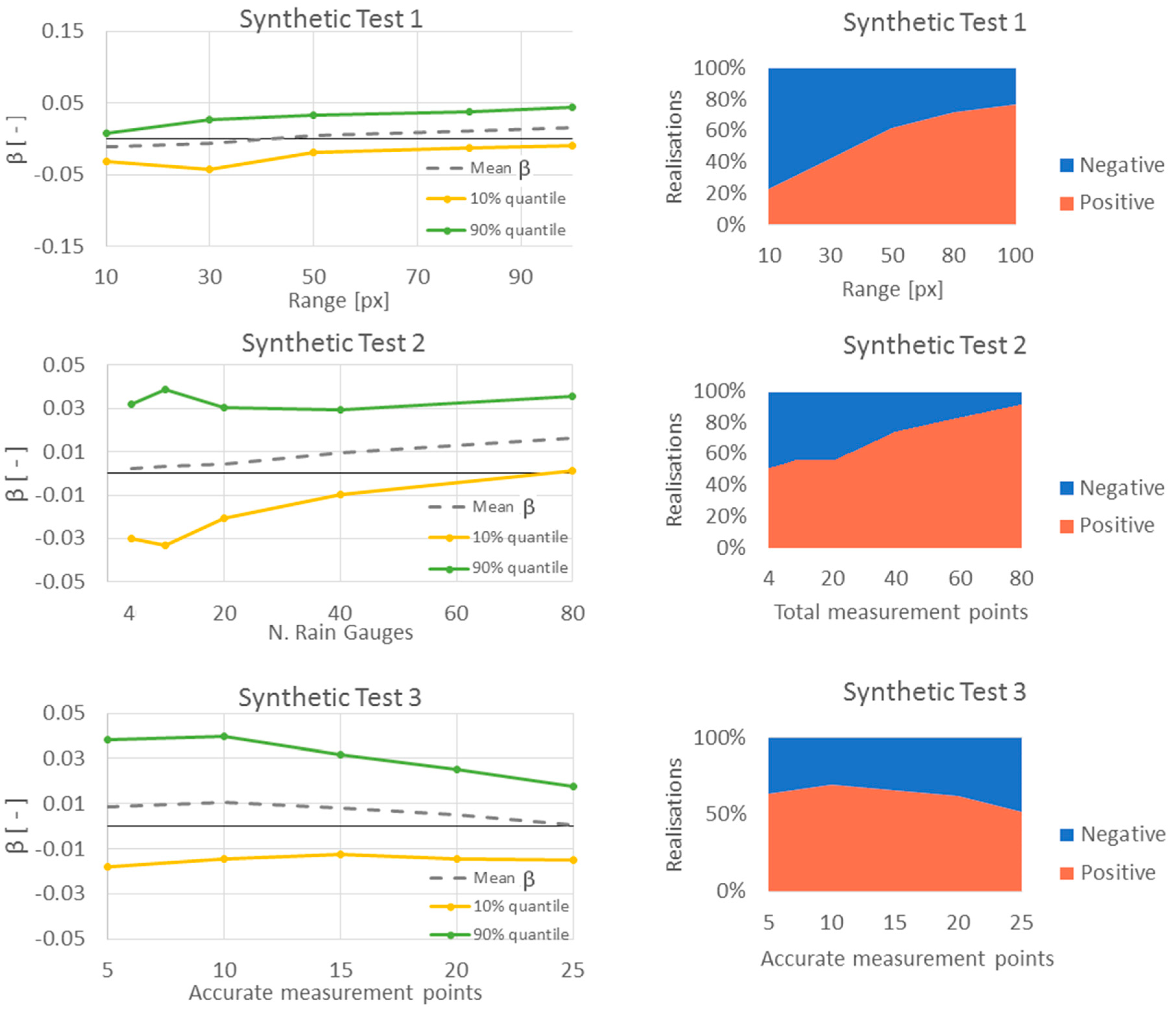
For each experiment, the average β, together with the 10% and 90% quantiles obtained out of the 500 realisations are presented in Figure 2, in the left plots. Additionally, the number of realisations with positive or negative β, indicating the number of times OKUD outperforms or underperforms OK, are reported in the right-side plots.
The results of the synthetic experiments reported in Figure 2 show some interesting outcomes. The first thing to notice is that in none of the analysed configurations OKUD performs consistently better or consistently worse than OK throughout the 500 realisations. This suggests that each combination of rain gauge configurations, error sampling and rainfall field behaves in a different way. The reason for this is that OKUD tends to smooth the field, giving less weight to the less accurate measurements. This has a positive effect if indeed the introduced error overestimates a peak or underestimate a low. Instead, the effect is counterproductive when it results in smoothing peaks and lows that were correctly estimated.
Figure 3 shows an example of a realisation, with 15 accurate and 15 less accurate rain gauges and a range of 50. In the figure, the first panel represents the generated field, the second represents the interpolation using OK and the third represents the OKUD interpolation. The value sampled by the rain gauges are superimposed, using the same scale.
Figure 3 shows some examples of the mechanism explained before. Two less accurate rain gauges in the bottom-left part of the panels are overestimating a peak and underestimating a low respectively; compared to the original field, the prediction obtained through OK overestimates the intensity in correspondence of the high-intensity measurement point and underestimate the intensity in the bottom-left corner, while OKUD smooths the field in both areas, getting closer to the real values. However, in the bottom-central part, a less accurate rain gauge correctly estimates a peak but OKUD smooths it. In such a situation OK outperforms OKUD. Similarly, the less accurate measurement in the top-central part of the panels measures low intensity; in OK the prediction estimates low intensity in the whole top-right corner, while OKUD smooths it to an average value. In such a case, the importance of the relative position of rain gauges is highlighted: the top-right corner is under-sampled, therefore none of the two methods is able to correctly estimate low and high intensity areas.
When a sufficient number of measuring points is available, in relation to the field spatial variability, OKUD is able to better estimate the direction of the errors and correct them, thanks to the comparison to adjacent measuring points; if instead the rain gauges are too sparse, in relation to the spatial variability of the field, OKUD may result in a loss of spatial information.
The results of the first experiment, reported in the top plots of Figure 2, show that OKUD performs better when a high range value is used. In such a situation, the fields θ are more homogeneous and a lower number of rain gauges is sufficient. In practical terms, the experiment suggests that OKUD could perform better for stratiform rainfall events or using coarser temporal resolutions and worse for convective rainfall or at fine temporal resolutions. The results of the second experiment, reported in the central panels of Figure 2, show that OKUD performs better with a higher rain gauge density. The reason for this behaviour is again that a higher number of rain gauges allows us to have a sufficient spatial sampling of the field, identifying highs and lows more precisely and balancing out the measurement errors. Another interesting feature that can be observed in the second experiment is that the variability of outcomes, represented by the difference between the 10% and 90% quantile, becomes lower for higher rain gauge densities. This means that the OKUD and OK results tend to converge to a better estimation of the field. Finally, the results of the third experiment, plotted in the lower panels of Figure 2, suggest that OKUD performs better than OK when the rain gauges have a more variable accuracy, when the difference between the number of accurate and less accurate rain gauges is lower. The OKUD method is able to give a higher weight to the good measurements and a lower weight to the less accurate ones. When the sampling points have a more uniform accuracy, this advantage is less important and the two methods perform more similarly, that is, the β mean is closer to zero. Again, the distribution is narrower for a higher number of accurate rain gauges, indicating that more accurate measurements result in a convergence of OKUD and OK results.
The presented synthetic experiment is necessary to study the characteristics of the KUD technique without the influence of other sources of uncertainty that are present in real case scenarios. However, it still has some limitations. Firstly, rainfall fields are not Gaussian. The use of a Gaussian field has been chosen to avoid the introduction of errors due to the application of an intrinsically Gaussian technique (Kriging) on non-Gaussian fields. To limit the impact of this choice on the applicability of the results to a real case, we used a differential evaluation system, as presented in Section 3.4.4, assuming that both OKUD and OK are affected in the same way by the use of Gaussian synthetic data. Another possible limitation is due to the independent simulation of rain gauge errors: although this design is suitable to represent random errors like blocking or mechanical failures, it does not capture the geographical correlation of errors due for example to orography, snowfall or intense precipitation on larger areas. The clustering of less accurate rain gauges could cause the KUD performances to drop and would justify even more the use of an additional spatial information, like the use of radar estimations in KED. To better understand if the results from the synthetic experiments are applicable to the real world, the real case study is presented, including results for OK and OKUD as well as KED and KEDUD.
4.2. Case Study Results and Discussion
The three deterministic indicators calculated through rain gauge validation for the four rainfall products used in the Dommel case study are reported in Table 3. The results of the case study application confirm the outcomes of the synthetic experiments. The deterministic validation, reported in Table 3, shows that OKUD performs slightly better than OK. It must be noted that in the real case there are a total of 13 rain gauges available, divided in 7 accurate KNMI automatic rain gauges and 6 less accurate rain gauges from the Dommel Water Board and from the Municipality of Eindhoven and the average range value for the semivariogram in the analysed time series is around 55.3 km. Therefore, the outcome of the real case study is expected to be similar to the outcome of the first synthetic experiment using a fixed range at 50 km, to the second experiment using a total number of rain gauges of 10 and to the third experiment using a balanced number of accurate and less accurate rain gauges. Indeed, in such situations the outcome of the three synthetic experiments show a tendency of OKUD to slightly outperform OK, as observed in the real case study. When the radar is used as a covariate in the real case study, the advantage in using KEDUD compared to KED becomes bigger than the advantage of OKUD compared to OK. This is due to the additional rainfall spatial information that the radar provides, which drives the model in reconstructing the rainfall field spatial features and avoiding excessive smoothing of the field.
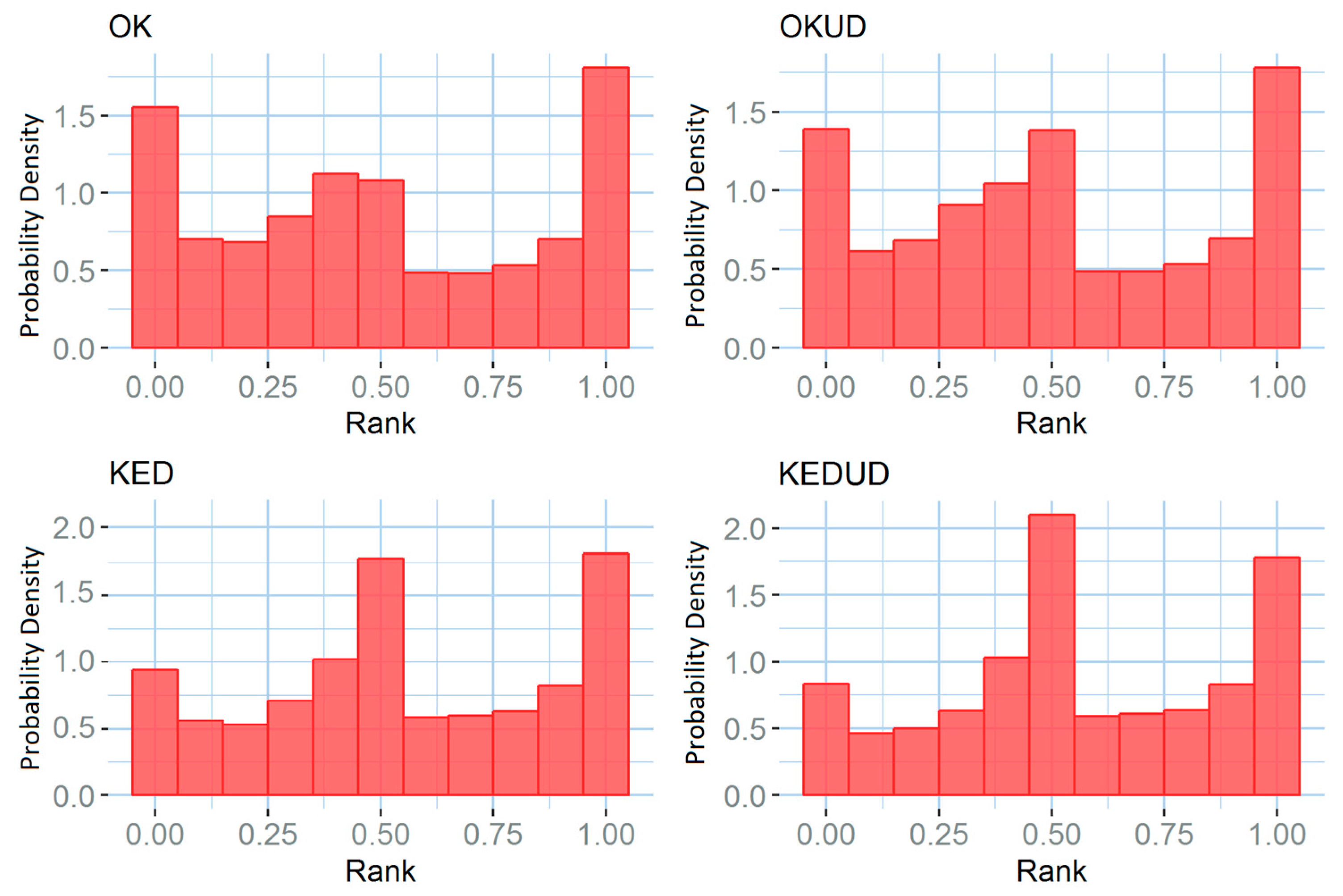
The rank histograms for the four products are reported in Figure 4.
Rank histogram are generated considering all the couples of observed value-probabilistic estimate. For each couple, the probabilistic estimate gives a probability distribution and it is noted in which quantile the observation falls. The rank histogram is built binning the quantiles in which the observation falls for all the available observation-estimation couples. In our case, the probabilistic estimation are the OK, OKUD, KED and KEDUD estimations. These are kriging based and assume a Gaussian probability distribution, described by a mean and a kriging variance. If the probabilistic estimation were perfect, the observations would fall in the respective quantiles proportionally to the expected probability and the rank histogram would result flat, that is, all bars would have the same height. However, this is not the case in our case study, as we know that the probability distribution of rainfall is not well described by the kriging Gaussian probability distribution. The fact that the Gaussian approximation is not a good representation of rainfall probability distribution is a known limitation of kriging methods [34,42]. However, the rank histograms can still be informative. The results represented in Figure 4 show that the KUD scheme tends to improve both the uncertainty estimation for OK and for KED. For all the cases, both the central quantiles and the extreme quantiles are higher than the other ones, which means that the real distribution of rainfall has a higher kurtosis than the Gaussian distribution with the modelled mean and variance. Both in the case of OKUD and KEDUD the bars corresponding to the first and in smaller measure to the last quantiles are reduced compared to the OK and KED cases. This means that the uncertainty estimation is improved and less observations fall outside the 10–90% uncertainty band. The fact that the central quantile is higher for OKUD and KEDUD reinforces the conclusions that rainfall kurtosis is higher than predicted by a Gaussian distribution, as more observation than expected fall in the central quantile and in the tail quantiles. This was less represented by the OK estimation. The fact that the difference is small is due to the fact that the rain gauge uncertainty is only a small part of the overall rainfall uncertainty and is not expected to explain all the difference between the modelled and the observed rainfall.
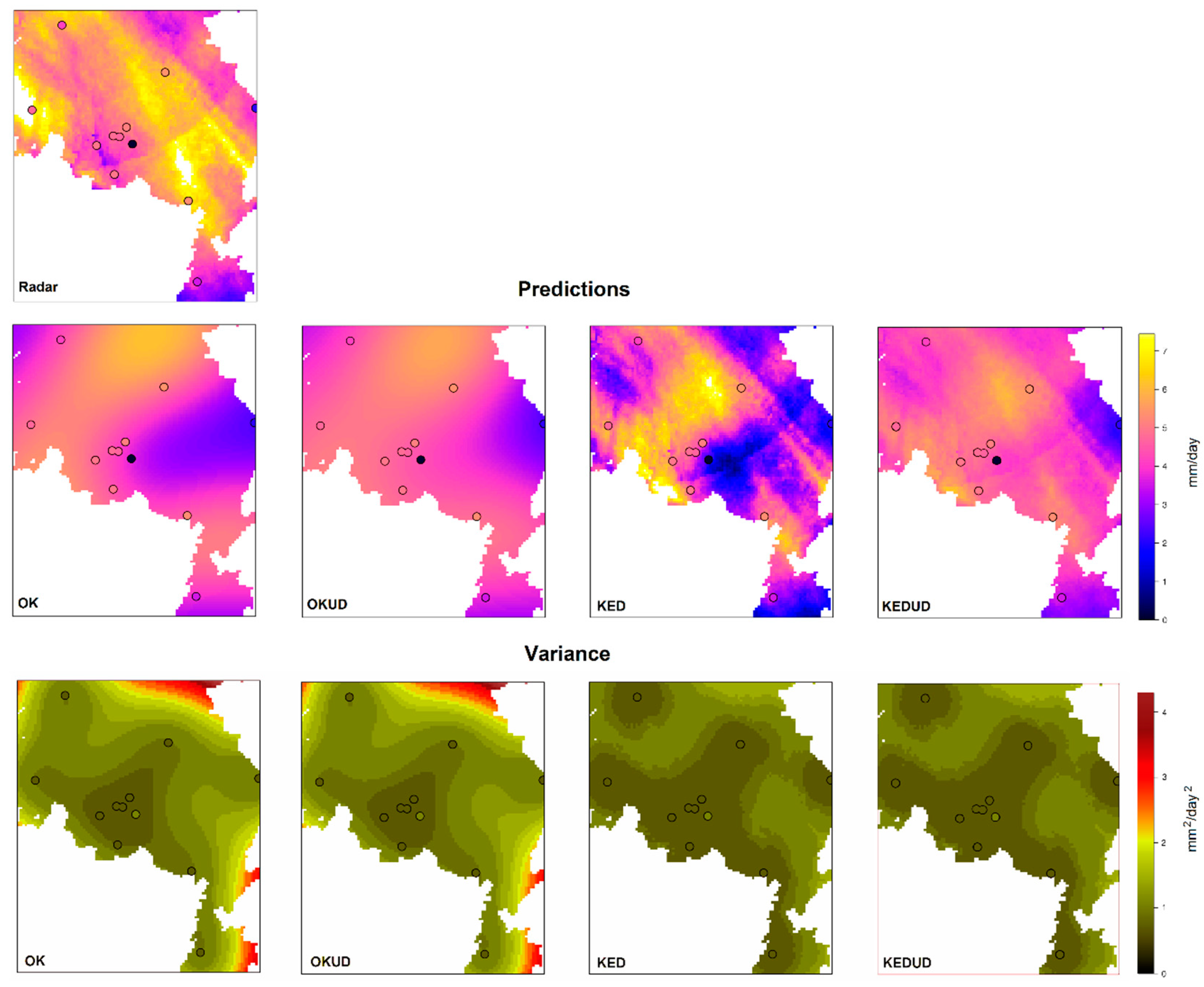
As a qualitative example, the rainfall accumulation between 8:00 (CET) of 23 January 2011 and the 8:00 (CET) of 24 January 2011 is used as an example, because one of the DWB rain gauges is malfunctioning and recorded no rainfall, in clear disagreement with the other rain gauges and the radar. This example of a rain gauge error highlights the effect of using KUD instead of the standard kriging. The products are compared in Figure 5. Rain gauge rainfall intensities are superimposed to the model predictions, while the estimated rain gauge nuggets are superimposed to the modelled kriging variance, in both cases using the same colour scale.
The KUD framework influences the variance but it has also an effect on the prediction, since the kriging weights are obtained minimising the variance. The use of different nugget effects for different networks reduces the weights for the less reliable rain gauges, which consequently have a lower influence on the kriging predictions. The effects of KUD on ordinary kriging and kriging with external drift are similar but with an important difference: the radar introduces additional rainfall spatial information that helps reconstructing the information lost giving a smaller weight to the less accurate data points. These effects can be observed in the example shown in Figure 5.
The event is selected because an observable error affects one of the rain gauges of the DWB network, namely “Eindhoven 1” in Figure 1, which recorded no rain, in clear disagreement with the other rain gauges and the radar estimation. Both the OK and the KED estimations try to accommodate the measurement of the “Eindhoven 1” rain gauge estimating a large low-intensity area at the centre of the study area, which disagrees with the radar QPE. The OKUD estimation partially reduces this effect. However, without the radar information it is impossible to reconstruct the high-intensity area estimated by the radar. The prediction of KEDUD instead can partially reconstruct the radar observation. It must be noted that, observing the other rain gauge measurements in comparison to the radar estimate, in the top-left panel, the radar is probably over-estimating rainfall in this temporal frame. Radar errors can be significant as well. However, thanks to KED using a linear function of the external drift, radar biases are implicitly corrected. Radar residual spatially-variant errors can still introduce some residual uncertainty in the final product. Nevertheless, the study or correction of these residual radar errors is complex and out of the scope of this work.
A final consideration can be made on the kriging variance estimations in the bottom four panels of Figure 5. The differences between the cases with and without the KUD framework in Figure 5 are not noticeable in the representation, which confirms that the rain gauge measurement errors are a small part of the overall rainfall error. However, the fact that the uncertainty estimation is not affected much by the measurement uncertainty does not mean that considering the measurement uncertainty is not important, as the observations on the rainfall kriging prediction results demonstrate.
5. Conclusions
It is widely recognised that merging radar and rain gauge rainfall information helps to improve rainfall estimates. Although rain gauges are known to be affected by a multitude of errors, often dependent on the rainfall intensity, rarely the measurement uncertainty is considered in merged radar-rain gauge rainfall products. When uncertainty is considered, it is often approximated with a stationary model, invariant in space and often invariant in time and independent from the rainfall intensity. This work investigates the use of kriging for uncertain data (KUD), coupled with rain gauge error models derived jointly by available experimental information, theoretical models and expert judgement, to include measurement uncertainty in the overall uncertainty estimation of kriging rainfall products. The uncertainty for each rain gauge is modelled separately and is a function of the rain gauge type, of the accumulation interval and of the rainfall intensity, therefore it is neither stationary in space nor in time. The overall rainfall uncertainty is estimated using the kriging variance. Two products are tested with and without KUD application: the use of OK and the use of KED using radar as covariate. Three synthetic experiments and one real case study demonstrate that the use of KUD tends to improve the rainfall estimations, both in terms of kriging predictions (better skill scores) and in terms of kriging variance (more realistic rank histograms). However, the use of KUD is not beneficial in the 100% of the cases, as not all the synthetic realisations showed a better performance of the KUD case; KUD it is not recommended in case of low rain gauge density and in case of high spatial variability of rainfall, for example in convective situations or at fine temporal resolution. This may be particularly important, as many modelling applications usually require sub-daily temporal scales. The use of radar as a covariate in KED improves the performance of KUD, because it restores the spatial information that can be lost considering some measurements less certain. In fact, kriging minimises the variance, which results in a smoothing of the field, especially close to rain gauge measurements that are considered more uncertain. The radar spatial information partially reconstructs the spatial structure of rainfall lost in the smoothing. Overall, rain gauge measurement uncertainty is a small part of the total rainfall uncertainty but its modelling is often beneficial not only in terms of uncertainty estimation but more importantly in terms of prediction improvement.
Author Contributions
Conceptualization, F.C. and A.M.M.-R.; Methodology, F.C. and A.M.M.-R.; Software, F.C. and A.M.M.-R.; Validation, F.C. and A.M.M.-R.; Formal Analysis, F.C.; Investigation, F.C. and A.M.M.-R.; Resources, F.C. and A.M.M.-R.; Data Curation, F.C. and A.M.M.-R.; Writing—Original Draft Preparation, F.C.; Writing—Review & Editing, F.C., A.M.M.-R., M.A.R.-R., M.-c.t.V. and J.G.L.; Visualization, F.C.; Supervision, M.A.R.-R. Veldhuis and J.G.L.; Funding Acquisition, M.A.R.-R., M.-c.t.V and J.G.L.., M.-c.t.V. and J.G.L.; Project Administration, M.A.R.-R., M-c.t.V.
Funding
This work was carried out in the framework of the Marie Skłodowska Curie Initial Training Network QUICS. The QUICS project has received funding from the European Union’s Seventh Framework Programme for research, technological development and demonstration under grant agreement no 607000. M.A. Rico-Ramirez also acknowledges the support of the Engineering and Physical Sciences Research Council (EPSRC) via Grant EP/I012222/1.
Acknowledgments
The authors would like to thank the KNMI, the Waterschap De Dommel and the Municipality of Eindhoven, which provided the radar rainfall data and the rain gauge data to develop this study. A special thank is also for Gerard Heuvelink from Wageningen University for the geostatistical expertise and for François Clemens, Petra Van Daal and Matthieu Spekkers, from TU Delft, for the advice on the Eindhoven catchment, the dataset and the data management.
Conflicts of Interest
The authors declare no conflict of interest. The funders had no role in the design of the study; in the collection, analyses, or interpretation of data; in the writing of the manuscript and in the decision to publish the results.
References
- Schilling, W. Rainfall data for urban hydrology: What do we need? Atmos. Res. 1991, 27, 5–21. [Google Scholar] [CrossRef]
- Berne, A.; Delrieu, G.; Creutin, J.; Obled, C. Temporal and spatial resolution of rainfall measurements required for urban hydrology. J. Hydrol. 2004, 299, 166–179. [Google Scholar] [CrossRef]
- Einfalt, T.; Arnbjerg-Nielsen, K.; Golz, C.; Jensen, N.; Quirmbach, M.; Vaes, G.; Vieux, B. Towards a roadmap for use of radar rainfall data in urban drainage. J. Hydrol. 2004, 299, 186–202. [Google Scholar] [CrossRef]
- Thorndahl, S.; Einfalt, T.; Willems, P.; Ellerbæk Nielsen, J.; Ten Veldhuis, M.C.; Arnbjerg-Nielsen, K.; Rasmussen, M.R.; Molnar, P. Weather radar rainfall data in urban hydrology. Hydrol. Earth Syst. Sci. 2017, 21, 1359–1380. [Google Scholar] [CrossRef] [Green Version]
- Goudenhoofdt, E.; Delobbe, L. Evaluation of radar-gauge merging methods for quantitative precipitation estimates. Hydrol. Earth Syst. Sci. Discuss. 2009, 5, 2975–3003. [Google Scholar] [CrossRef]
- Berndt, C.; Rabiei, E.; Haberlandt, U. Geostatistical merging of rain gauge and radar data for high temporal resolutions and various station density scenarios. J. Hydrol. 2014, 508, 88–101. [Google Scholar] [CrossRef]
- Jewell, S.A.; Gaussiat, N. An assessment of kriging-based rain-gauge-radar merging techniques. Q. J. R. Meteorol. Soc. 2015, 141, 2300–2313. [Google Scholar] [CrossRef]
- Clark, I. Statistics or geostatistics? Sampling error or nugget effect? J. S. Afr. Inst. Min. Metall. 2010, 110, 307–312. [Google Scholar]
- Cressie, N.A.C. Statistics for Spatial Data, Revised ed.; Kohn Wiley & Sons: New York, NY, USA, 1993. [Google Scholar]
- Germann, U.; Berenguer, M.; Sempere-Torres, D.; Zappa, M. REAL—Ensemble radar precipitation estimation for hydrology in mountainous region. Q. J. R. Meteorol. Soc. 2009, 135, 445–456. [Google Scholar] [CrossRef] [Green Version]
- Villarini, G.; Krajewski, W.F. Empirically based modelling of radar-rainfall uncertainties for a C-band radar at different time-scales. Q. J. R. Meteorol. Soc. 2009, 1438, 1424–1438. [Google Scholar] [CrossRef]
- Ciach, G.J.; Krajewski, W.F.; Villarini, G. Product-Error-Driven Uncertainty Model for Probabilistic Quantitative Precipitation Estimation with NEXRAD Data. J. Hydrometeorol. 2007, 8, 1325–1347. [Google Scholar] [CrossRef]
- Rico-Ramirez, M.A.; Liguori, S.; Schellart, A.N.A. Quantifying radar-rainfall uncertainties in urban drainage flow modelling. J. Hydrol. 2015, 528, 17–28. [Google Scholar] [CrossRef]
- Sevruk, B. Adjustment of tipping-bucket precipitation gauge measurements. Atmos. Res. 1996, 42, 237–246. [Google Scholar] [CrossRef]
- Nešpor, V.; Sevruk, B. Estimation of wind-induced error of rainfall gauge measurements using a numerical simulation. J. Atmos. Ocean. Technol. 1999, 16, 450–464. [Google Scholar] [CrossRef]
- Habib, E.H.; Meselhe, E.A.; Aduvala, A. V Effect of Local Errors of Tipping-Bucket Rain Gauges on Rainfall-Runoff Simulations. J. Hydrol. Eng. 2008, 13, 488–496. [Google Scholar] [CrossRef]
- Molini, A.; Lanza, L.G.; La Barbera, P. The impact of tipping-bucket raingauge measurement errors on design rainfall for urban-scale applications. Hydrol. Process. 2005, 19, 1073–1088. [Google Scholar] [CrossRef]
- Steiner, M.; Smith, J.A.; Burges, S.J.; Alonso, C.V.; Darden, R.W. Effect of bias adjustment and rain gauge data quality control on radar rainfall estimation. Water Resour. Res. 1999, 35, 2487–2503. [Google Scholar] [CrossRef] [Green Version]
- Peleg, N.; Ben-Asher, M.; Morin, E. Radar subpixel-scale rainfall variability and uncertainty: Lessons learned from observations of a dense rain-gauge network. Hydrol. Earth Syst. Sci. 2013, 17, 2195–2208. [Google Scholar] [CrossRef]
- Villarini, G.; Mandapaka, P.V.; Krajewski, W.F.; Moore, R.J. Rainfall and sampling uncertainties: A rain gauge perspective. J. Geophys. Res. 2008, 113, D11102. [Google Scholar] [CrossRef]
- Upton, G.J.G.; Rahimi, A.R. On-line detection of errors in tipping-bucket raingauges. J. Hydrol. 2003, 278, 197–212. [Google Scholar] [CrossRef] [Green Version]
- Luyckx, G.; Berlamont, J. Simplified Method to Correct Rainfall Measurements from Tipping Bucket Rain Gauges. In Proceedings of the World Water and Environmental Resources Congress, Orlando, FL, USA, 20–24 May 2001; pp. 767–776. [Google Scholar]
- Ciach, G.J. Local Random Errors in Tipping-Bucket Rain Gauge Measurements. J. Atmos. Ocean. Technol. 2003, 20, 752–759. [Google Scholar] [CrossRef]
- Lebel, T.; Bastin, G.; Obled, C.; Creutin, J.D. On the accuracy of areal rainfall estimation: A. case study. Water Resour. Res. 1987, 23, 2123–2134. [Google Scholar] [CrossRef]
- Habib, E.; Ciach, G.J.; Krajewski, W.F. A method for filtering out raingauge representativeness errors from the verification distributions of radar and raingauge rainfall. Adv. Water Resour. 2004, 27, 967–980. [Google Scholar] [CrossRef]
- Hasan, M.M.; Sharma, A.; Johnson, F.; Mariethoz, G.; Seed, A. Correcting bias in radar Z–R relationships due to uncertainty in point rain gauge networks. J. Hydrol. 2014, 519, 1668–1676. [Google Scholar] [CrossRef]
- Bringi, V.N.; Rico-Ramirez, M.A.; Thurai, M. Rainfall Estimation with an Operational Polarimetric C-Band Radar in the United Kingdom: Comparison with a Gauge Network and Error Analysis. J. Hydrometeorol. 2011, 12, 935–954. [Google Scholar] [CrossRef]
- De Marsily, G. Quantitative Hydrogeology, 1st ed.; Academic Press: San Diego, CA, USA, 1986. [Google Scholar]
- Mazzetti, C.; Todini, E. Combining Weather Radar and Raingauge Data for Hydrologic Applications. In Flood Risk Management: Research and Practice; Samuels, P., Huntington, S., Allsop, W., Harrop, J., Eds.; Taylor & Francis Group: London, UK, 2009; ISBN 9780415485074. [Google Scholar]
- Krajewski, W.F.; Ciach, G.J. Towards Probabilistic Quantitative Precipitation WSR-88D Algorithms: Preliminary Studies and Problem Formulation; National Oceanic and Atmospheric Administration/National Weather Service: Iowa City, IA, USA, 2003; p. 59.
- Brandsma, T. Comparison of Automatic and Manual Precipitation Networks in The Netherlands; Royal Netherlands Meteorological Institute: De Bilt, The Netherlands, 2014; p. 42. [Google Scholar]
- Wauben, W. WMO Laboratory Intercomparison of Rainfall Intensity Gauges; Instrumental Department, INSA-IO, KNMI: De Bilt, the Netherlands, 2006; p. 164. [Google Scholar]
- Overeem, A.; Holleman, I.; Buishand, A. Derivation of a 10-Year Radar-Based Climatology of Rainfall. J. Appl. Meteorol. Climatol. 2009, 48, 1448–1463. [Google Scholar] [CrossRef]
- Cecinati, F.; Wani, O.; Rico-Ramirez, M.A. Comparing Approaches to Deal With Non-Gaussianity of Rainfall Data in Kriging-Based Radar-Gauge Rainfall Merging. Water Resour. Res. 2017. [Google Scholar] [CrossRef]
- Marcotte, D. Fast variogram computation with FFT. Comput. Geosci. 1996, 22, 1175–1180. [Google Scholar] [CrossRef]
- Nerini, D.; Besic, N.; Sideris, I.; Germann, U.; Foresti, L. A non-stationary stochastic ensemble generator for radar rainfall fields based on the short-space Fourier transform. Hydrol. Earth Syst. Sci. 2017, 21, 2777–2797. [Google Scholar] [CrossRef] [Green Version]
- Velasco-Forero, C.A.; Sempere-Torres, D.; Cassiraga, E.F.; Gómez-Hernández, J.J. A non-parametric automatic blending methodology to estimate rainfall fields from rain gauge and radar data. Adv. Water Resour. 2009, 32, 986–1002. [Google Scholar] [CrossRef]
- Habib, E.; Krajewski, W.F.; Kruger, A. Sampling Errors of Tipping-Bucket Rain Gauge Measurements. J. Hydrol. Eng. 2001, 6, 159–166. [Google Scholar] [CrossRef]
- Cecinati, F.; de Niet, A.; Sawicka, K.; Rico-Ramirez, M.A. Optimal Temporal Resolution of Rainfall for Urban Applications and Uncertainty Propagation. Water 2017, 9, 762. [Google Scholar] [CrossRef]
- Hamill, T.M. Interpretation of Rank Histograms for Verifying Ensemble Forecasts. Mon. Weather Rev. 2001, 129, 550–560. [Google Scholar] [CrossRef] [Green Version]
- Cecinati, F.; Moreno Ródenas, A.M.; Rico-Ramirez, M.A. Integration of rain gauge errors in radar-rain gauge merging techniques. In Proceedings of the 10th World Congress on Water Resources and Environment, Athens, Greece, 8 July 2017; pp. 279–285. [Google Scholar]
- Erdin, R.; Frei, C.; Künsch, H.R. Data Transformation and Uncertainty in Geostatistical Combination of Radar and Rain Gauges. J. Hydrometeorol. 2012, 13, 1332–1346. [Google Scholar] [CrossRef]
Figure 1.
The Figure shows the position of the rain gauges and of the Dommel catchment inside the study area on the left; the position of the radars and of the study area (black rectangle) relatively to the Netherlands on the right.
Figure 1.
The Figure shows the position of the rain gauges and of the Dommel catchment inside the study area on the left; the position of the radars and of the study area (black rectangle) relatively to the Netherlands on the right.

Figure 2.
For each experiment, two plots are reported; the ones on the left show the mean, the 10% and 90% quantiles of the β values. The plots on the right show how many times OKUD outperforms OK (positive β) and how many times instead OK outperforms OKUD (negative β). For the Synthetic Test 3, only the number of accurate points is reported on the horizontal axis. Please note that the figure is from [41] as a shorter version of the work was presented at the EWRA conference 2017.

Figure 3.
Example of a synthetic field generated during the third experiment. 15 accurate rain gauges (bordered in black) and 15 less accurate rain gauges (bordered in grey) are used to sample the field and the values are superimposed.
Figure 3.
Example of a synthetic field generated during the third experiment. 15 accurate rain gauges (bordered in black) and 15 less accurate rain gauges (bordered in grey) are used to sample the field and the values are superimposed.

Figure 4.
Rank histograms relative to the four studied rainfall products.

Figure 5.
Kriging prediction and kriging variance for each of the four rainfall products. Rain gauge rainfall intensities and rain gauge estimated nuggets are superimposed to the kriging predictions and to the kriging variance, respectively, using the same colour scales. The top-left panel shows the radar rainfall estimation used for KED and KEDUD.


Table 1.
Summary of the available rain gauge networks, their characteristics and how they are used in this work.
Table 1.
Summary of the available rain gauge networks, their characteristics and how they are used in this work.
| ID | Provider | Use | Number | Type | Temporal Resolution | Intensity resolution |
|---|---|---|---|---|---|---|
| EM | Municipality of Eindhoven | Modelling | 3 | Tipping bucket | 1 min | 0.25 mm |
| DWB | Dommel Water Board | Modelling | 3 | Tipping bucket | 1 min | 0.1 mm |
| KNMI-A | KNMI | Modelling | 7 | Floating device | 12 s | 0.001 mm |
| KNMI-M | KNMI | Validation | 35 | Manual | 1 day | 0.1 mm |
Table 2.
Overview of the three experimental setups.
| Experiment 1 | Experiment 2 | Experiment 3 | |
|---|---|---|---|
| Tested variable | Range | Number of rain gauges | Accurate/less accurate rain gauge ratio |
| Tested values | (10, 30, 50, 80, 100) | (4, 10, 20, 40, 80) | (5/25, 10/20, 15/15, 20/10, 25/5) |
| Number of realisation | 500 for each range value | 500 for each tested number of rain gauges | 500 for each tested rain gauge ratio |
| Number of accurate rain gauges | 10 | 2, 5, 10, 20, 40 | 5, 10, 15, 20, 25 |
| Number of less accurate rain gauges | 10 | 2, 5, 10, 20, 40 | 25, 20, 15, 10, 5 |
| Range value [pixels] | 10, 30, 50, 80, 100 | 50 | 50 |
| Sill [ ] | 0.1 | 0.1 | 0.1 |
| Mean [ ] | 1 | 1 | 1 |
Table 3.
Deterministic validation results for the four tested rainfall products, in terms of RMSE, MRTE and bias.
Table 3.
Deterministic validation results for the four tested rainfall products, in terms of RMSE, MRTE and bias.
| RMSE | MRTE | BIAS | |
|---|---|---|---|
| OK | 2.49 | 0.32 | −0.38 |
| OKUD | 2.46 | 0.30 | −0.35 |
| KED | 2.48 | 0.28 | −0.39 |
| KEDUD | 2.08 | 0.22 | −0.37 |
© 2018 by the authors. Licensee MDPI, Basel, Switzerland. This article is an open access article distributed under the terms and conditions of the Creative Commons Attribution (CC BY) license (http://creativecommons.org/licenses/by/4.0/).
Share and Cite
MDPI and ACS Style
Cecinati, F.; Moreno-Ródenas, A.M.; Rico-Ramirez, M.A.; Ten Veldhuis, M.-c.; Langeveld, J.G. Considering Rain Gauge Uncertainty Using Kriging for Uncertain Data. Atmosphere 2018, 9, 446. https://doi.org/10.3390/atmos9110446
AMA Style
Cecinati F, Moreno-Ródenas AM, Rico-Ramirez MA, Ten Veldhuis M-c, Langeveld JG. Considering Rain Gauge Uncertainty Using Kriging for Uncertain Data. Atmosphere. 2018; 9(11):446. https://doi.org/10.3390/atmos9110446
Chicago/Turabian StyleCecinati, Francesca, Antonio M. Moreno-Ródenas, Miguel A. Rico-Ramirez, Marie-claire Ten Veldhuis, and Jeroen G. Langeveld. 2018. "Considering Rain Gauge Uncertainty Using Kriging for Uncertain Data" Atmosphere 9, no. 11: 446. https://doi.org/10.3390/atmos9110446
Note that from the first issue of 2016, this journal uses article numbers instead of page numbers. See further details here.