Article

Deterministic Greedy Routing with Guaranteed Delivery in 3D Wireless Sensor Networks

1
Cisco Systems, Milpitas, CA 95035, USA
2
Mathematics Department, Harvard University, Cambridge, MA 02138, USA
3
The Center for Advanced Computer Studies, University of Louisiana, Lafayette, LA 70504, USA
4
Department of Computer Science, Stony Brook University, Stony Brook, NY 11790, USA
*
Author to whom correspondence should be addressed.
Axioms 2014, 3(2), 177-201; https://doi.org/10.3390/axioms3020177
Submission received: 22 February 2014 / Revised: 25 April 2014 / Accepted: 28 April 2014 / Published: 15 May 2014

Abstract

:
With both computational complexity and storage space bounded by a small constant, greedy routing is recognized as an appealing approach to support scalable routing in wireless sensor networks. However, significant challenges have been encountered in extending greedy routing from 2D to 3D space. In this research, we develop decentralized solutions to achieve greedy routing in 3D sensor networks. Our proposed approach is based on a unit tetrahedron cell (UTC) mesh structure. We propose a distributed algorithm to realize volumetric harmonic mapping (VHM) of the UTC mesh under spherical boundary condition. It is a one-to-one map that yields virtual coordinates for each node in the network without or with one internal hole. Since a boundary has been mapped to a sphere, node-based greedy routing is always successful thereon. At the same time, we exploit the UTC mesh to develop a face-based greedy routing algorithm and prove its success at internal nodes. To deliver a data packet to its destination, face-based and node-based greedy routing algorithms are employed alternately at internal and boundary UTCs, respectively. For networks with multiple internal holes, a segmentation and tunnel-based routing strategy is proposed on top of VHM to support global end-to-end routing. As far as we know, this is the first work that realizes truly deterministic routing with constant-bounded storage and computation in general 3D wireless sensor networks.

Graphical Abstract

1. Introduction

With both its computational complexity and storage space bounded by a small constant, greedy routing is known for its scalability to large networks with stringent resource constraints on individual nodes. Under most greedy routing algorithms, a node makes its routing decision by standard distance calculation based on a small set of local coordinates only. Such a salient property is imperatively needed in emerging 3D sensor networks [1,2,3,4,5,6,7,8,9,10,11,12], where the problem in routing scalability is greatly exacerbated in comparison with its 2D counterpart, due to dramatically increased sensor nodes in order to cover a 3D space.
The conventional greedy routing algorithms are node-based [13,14]. More specifically, a node always forwards a packet to one of its neighbors, which is the closest to the destination of the packet. However, such greedy forwarding is not always achievable. A node is called a local minimum if it is not the destination, but closer to the destination than all of its neighbors. Clearly, greedy routing fails at the local minimum. Such local minimums may appear at either boundary or internal nodes (as highlighted in red in Figure 1b). A node on a boundary, especially a concave boundary, usually becomes a local minimum when the source and destination nodes are located on two sides of the boundary. Although it seems anti-intuitive, an internal node can be a local minimum, too, due to local concavity under random deployment of sensor nodes.
Various approaches have been developed to address the problem of local minimum in 2D networks, with primary focus on boundaries. For example, face routing and its alternatives and enhancements [13,14,15,16,17,18,19,20] exploit the fact that a concave void in a 2D planar network is a face with a simple line boundary. Thus, when a packet reaches a local minimum on a boundary, it employs a local deterministic algorithm to search the boundary in either the clockwise or counter-clockwise direction, as shown in Figure 2a, until greedy forwarding is achievable. In a 3D network, however, a void is no longer a face. Its boundary becomes a surface, yielding an arbitrarily large number of possible paths to be explored (see Figure 2b) and, thus, rendering face routing infeasible. On the other hand, greedy embedding [21,22,23,24,25,26,27] provides theoretically sound solutions to ensure the success of greedy routing. Unfortunately, none of the greedy embedding algorithms in the literature can be extended from 2D to 3D general networks. The challenge of greedy routing in 3D networks is further revealed in [28], which proves that there does not exist a deterministic algorithm that can guarantee delivery based on local information only in 3D networks.
In view of the above challenges, several approaches have been proposed for recovery from local minimums in 3D networks. First, mapping and projection are introduced to reduce routing complexity in a 3D space. For example, a 3D network is projected to a 2D plane in [4,5] in order to apply face routing. However, face routing on the projected plane does not ensure that a packet moves out of a void in the original 3D network. A different projection scheme is proposed in [7] for load balancing, which does not guarantee delivery either. Second, guaranteed delivery can be achieved at the cost of more (non-constant-bounded) storage space. For example, a convex hull-based tree structure is introduced in GDSTR-3D [8]. A packet is greedily forwarded to its destination. If a local minimum is reached, GDSTR-3D switches to forwarding the packet along the edges of a spanning tree, guiding the packet to escape from the local minimum. GDSTR-3D offers deterministic routing. However, each node must maintain a set of convex hulls and, thus, requires a storage space proportional to network size, and some nodes (such as the roots of trees) are heavily loaded (see Figure 3). Finally, local searching may be employed to jump out of a local minimum. It is proposed in [3] to construct hulls to partition a network into subspaces, limiting the recovery to search a subspace only. Separately, the random-walk algorithm is proposed in [6], where random walk is employed on a local spherical structure to escape from voids when a local minimum is reached. However, such attempts for randomized recovery of local minimums are non-deterministic and often lead to high overhead or long delay. Among all routing algorithms discussed in the literature for 3D sensor networks, random-walk [6] is the sole truly greedy routing scheme with constant-bounded storage and computation complexity.
Figure 1. Illustration of the proposed greedy routing protocol. (a) A 3D sensor network that has irregular outer and inner boundaries and consists of about 2 , 000 nodes. This is one of the network models used in our simulation (see Figure 6 and Figure 8 for other network models). The nodes on the inner boundary are highlighted in red. (b) The nodes that are local minimums under node-based greedy routing are highlighted as blue squares and red triangles, for boundary nodes and internal nodes, respectively. (c) The established unit tetrahedron cells (UTCs). (d) The result after volumetric harmonic mapping, with both outer and inner boundaries mapped to spheres. (e) A greedy routing path shown in virtual coordinates created by volumetric harmonic mapping. (f) The greedy routing path shown in the original network.
Axioms 03 00177 g001
Figure 2. Comparison of face routing in 2D and 3D networks. Node S has a shorter distance to destination, D, than all of its neighbors and, thus, is a local minimum. (a) Face routing is successful in a 2D planar network, because a concave void is a face with a simple line boundary and, thus, a local deterministic algorithm can be employed to search the boundary in either the clockwise or counter-clockwise direction, as shown by the blue and red lines. (b) In a 3D network, a void is no longer a face. Its boundary becomes a surface, yielding an arbitrarily large number of possible paths to be explored (as indicated by the arrows). Thus, face routing fails.
Axioms 03 00177 g002
Figure 3. The storage load distribution in GDSTR-3D, where the storage load of a node is measured by the number of entries in its local convex hull table.
Axioms 03 00177 g003
Our proposed solution is based on a unit tetrahedron cell (UTC) mesh structure. We propose a distributed algorithm to realize volumetric harmonic mapping of the UTC mesh under a spherical boundary condition. It is a one-to-one map that yields virtual coordinates for each node in the network. Since a boundary has been mapped to a sphere, node-based greedy routing is always successful thereon. At the same time, we exploit the UTC mesh to develop a face-based greedy routing algorithm and prove its success at internal nodes. To route a data packet to its destination, face-based and node-based greedy routing algorithms are employed alternately at internal and boundary UTCs, respectively. For networks with multiple internal holes, a segmentation and tunnel-based routing strategy is proposed on top of VHM to support global end-to-end routing. As far as we know, this is the first work that realizes truly deterministic routing with constant-bounded storage and computation in general 3D sensor networks. To make a local routing decision, each node only needs to store virtual coordinates of itself and its neighbors and a routing table with a size bounded by the number of internal holes.
The rest of this paper is organized as follows: Section 2 introduces the construction of UTC and related definitions. Section 3 proposes the face-based greedy routing algorithm. Section 4 elaborates the distributed volumetric harmonic mapping algorithm that yields virtual coordinates to enable greedy routing for a network with no more than one hole. Section 5 proposes the scheme to support global end-to-end routing for networks with multiple internal holes by employing segmentation and tunnel-based routing. Section 6 presents our simulation results. Finally, Section 7 concludes the paper.

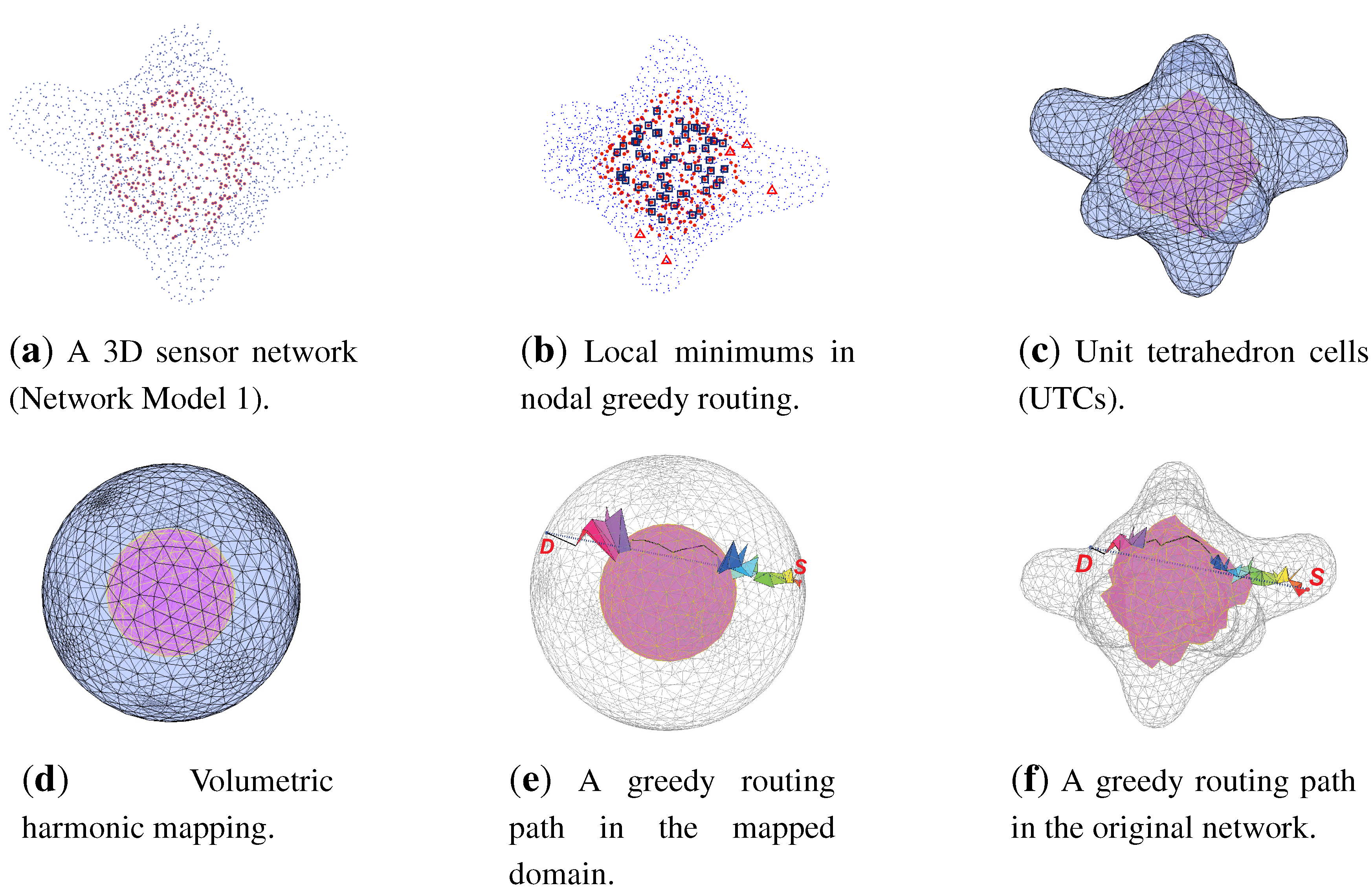
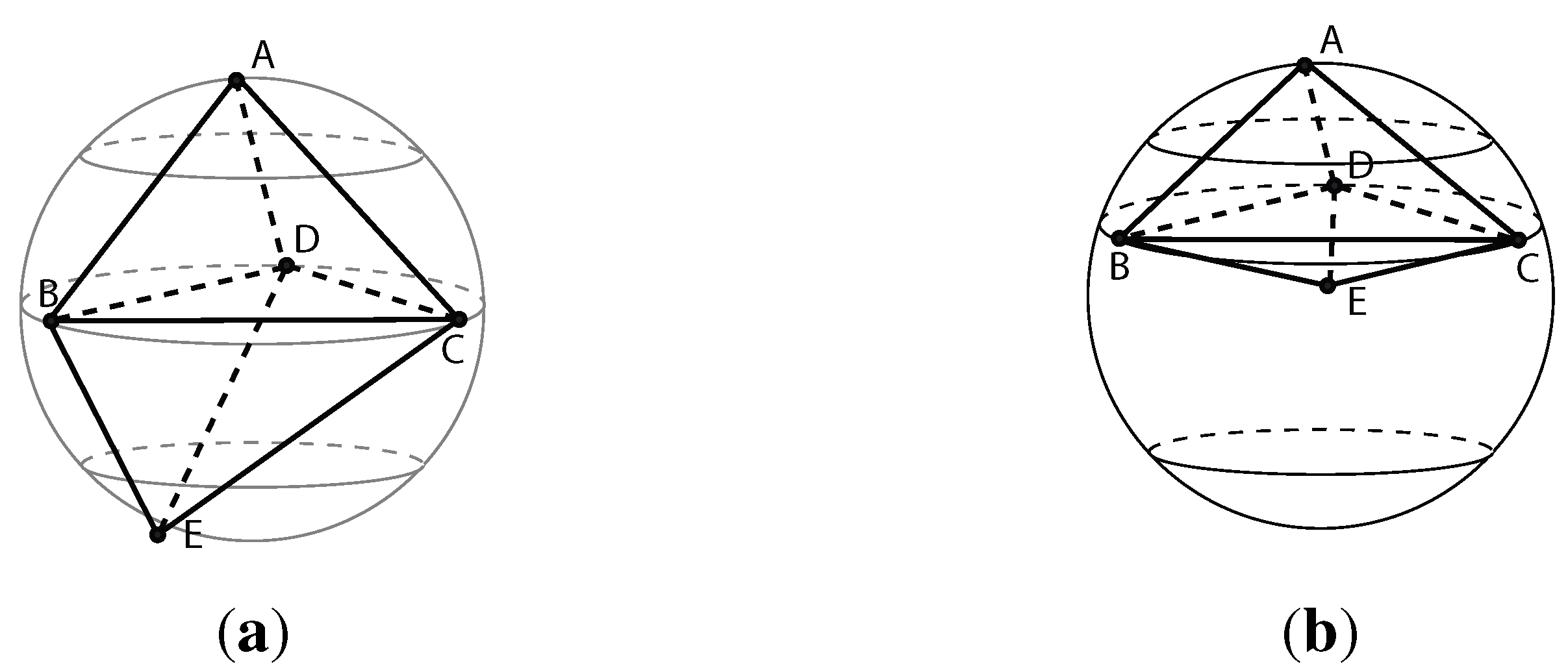
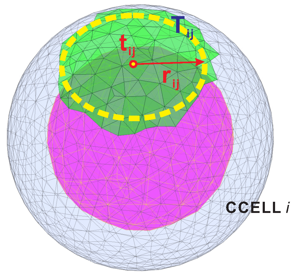
2. Construction of Unit Tetrahedron Cells

We represent a wireless sensor network by a graph, G ( V , E ) , where the vertices (V) denote the sensor nodes and the edges (E) indicate the communication links in the network.
Definition 1
A unit tetrahedron cell (UTC) is a tetrahedron formed by four network nodes, which does not intersect with any other tetrahedrons.
We let U T C ( A , B , C , D ) denote the UTC formed by Nodes A, B, C and D, which includes four faces, i.e., F a c e ( A , B , C ) , F a c e ( A , B , D ) , F a c e ( A , C , D ) and F a c e ( B , C , D ) . The union of all UTCs, called a UTC mesh (see Figure 1c), represent the network.
A simple algorithm is employed to create a UTC mesh, which starts from any arbitrary tetrahedron that contains its own vertex nodes only. By removing all edges that intersect this tetrahedron, the algorithm yields the first UTC, denoted by U T C ( A , B , C , D ) . Next, the algorithm expands it to form other UTCs. Based on each face of U T C ( A , B , C , D ) , such as F a c e ( A , B , C ) , the algorithm looks for the common neighbors of Nodes A, B and C. Let E be such a common neighbor. Nodes A, B, C and E form a valid UTC only if it neither overlaps with any existing UTCs nor contains any other nodes. Multiple such nodes, like E, may exist, and the algorithm arbitrarily chooses one of them to form the new UTC. The algorithm repeats the above procedure, until no new UTC can be formed.
Here, we have assumed that no degenerated edges or nodes exist in the network, and any internal hole (as small as a unit cube) has been identified by [29] to ensure the successful establishment of the UTC mesh. Moreover, we assume a node can create a local coordinates system by using local distance information estimated via standard methods [30]. Multiple available schemes are available for creating such a local coordinates system [31,32,33,34]. Our implementation adopts [34] for its efficiency of filtering noises in distance measurement and its tolerance of distance errors.
Definition 2
A Delaunay unit tetrahedron cell (DUTC) is a UTC whose circumsphere contains no other nodes, except its vertices.
For example, U T C ( A , B , C , D ) , shown in Figure 4a, is a DUTC, since its circumsphere contains no nodes, except A , B , C and D. On the other hand, Figure 4b illustrates U T C ( A , B , C , D ) that is not a DUTC, because Node E is inside its circumsphere. Similarly, neither is U T C ( E , B , C , D ) a DUTC. Note that the UTCs constructed by the algorithm introduced above are not necessarily DUTCs.
Definition 3
A face is a boundary face if it is contained in one UTC only.
Definition 4
A UTC is a boundary UTC if it contains at least one boundary face. A non-boundary UTC is call an internal UTC.
Figure 4. Illustration of a Delaunay unit tetrahedron cell (DUTC), under an arbitrary (non-unit disk graph (UDG)) communication model. (a) DUTC; (b) non-DUTC.
Axioms 03 00177 g004
Definition 5
A hole of a network is formed by a closed surface that consists of boundary faces. The outer boundary of the network is considered as a special hole.
For example, a set of boundary faces are highlighted in magenta in Figure 1c, which, together, form the surface of the hole.
Definition 6
Two UTCs are neighbors if and only if they share a face.
Apparently, a U T C has at most four neighboring U T C s . Similarly, we have:
Definition 7
Two faces are neighbors if and only if they share an edge.
Definition 8
Node i is greedily reachable to Node j if a packet can be greedily routed from the former to the latter based on a metric that is kept locally and consumes constant storage space.
Our objective is to enable greedy routing from any source to any destination in a given sensor network. More specifically, we aim to map an arbitrary 3D sensor network to a greedily reachable network, as defined below:
Definition 9
A network is called a greedily reachable network if every two nodes in the network are greedily reachable to each other.
Based on the above definitions, we next discuss how to enable a greedily reachable network. We first examine a simple case, i.e., greedy routing at internal nodes, which appears trivial, but is anti-intuitively unachievable by the straightforward application of the node-based greedy routing algorithm. Then, we introduce our proposed approach based on volumetric harmonic mapping for global end-to-end greedy routing.

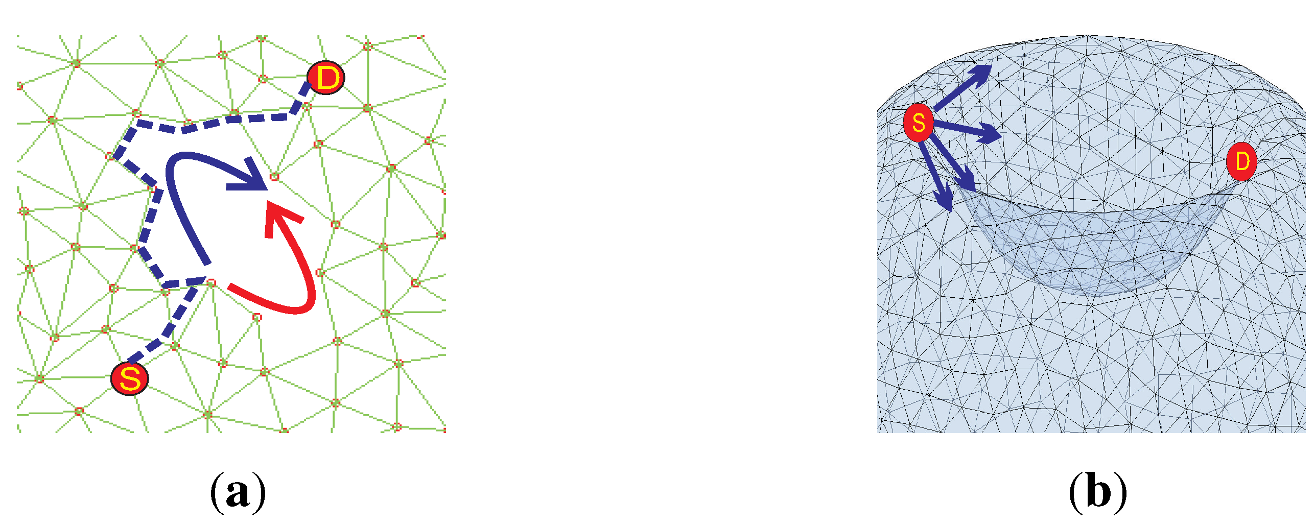
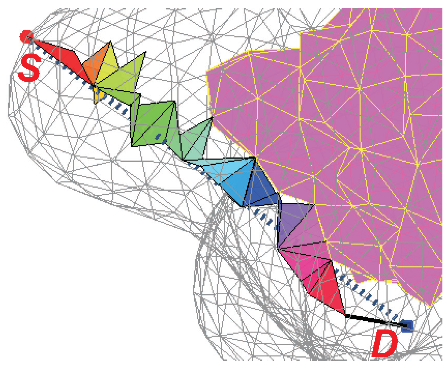
3. Routing at Internal UTCs: Face-Based Greedy Routing

As discussed in Section 1 and demonstrated in Figure 1b, the node-based greedy routing scheme ensures success at neither boundary nor internal nodes in a 3D wireless sensor network. We focus on the latter in this section.
We first show that node-based greedy routing is not always successful even under the UTC structure, for example, in a case as simple as across two neighboring UTCs. More specifically, let us consider two UTCs, U T C ( A , B , C , D ) and U T C ( B , C , D , E ) , which share F a c e ( B , C , D ) . If they are DUTCs, as illustrated in Figure 4a, Nodes A and E are greedily reachable to each other. However, building DUTCs is expensive and often impractical in sensor networks. The UTCs constructed by the algorithm introduced in Section 2 are not necessarily DUTCs. For a UTC shown in Figure 4b, for example, l E A can be shorter than l B A , l C A and l D A (where l i j denotes the distance between Nodes i and j), thus resulting in a failure in node-based greedy routing from E to A. Obviously, the UTC mesh is a special structure of a 3D sensor network. Since the node-based greedy routing is not always successful under UTCs, it offers no guarantee of data delivery in a general 3D sensor network either.
To this end, we propose a face-based greedy routing algorithm. Let us consider a data packet that is to be delivered from Source S to Destination D. Similar to conventional node-based greedy routing algorithms, we assume the data packet contains the IDs and coordinates of S and D. Note that the coordinates are not necessarily based on GPS. Instead, they can be virtual coordinates, e.g., produced by our proposed volumetric harmonic mapping algorithm, to be discussed later in Section 4.
Node S first computes a line segment between S and D, which is denoted by Γ. Clearly, Γ passes through a set of UTCs between S and D and intersects with a sequence of faces, denoted by Φ = { F a c e ( A i , B i , C i ) | 1 i k } , where k is the total number of such faces (see Figure 5). The distance from F a c e ( A i , B i , C i ) to destination D is defined as the distance between D and the intersection point of Γ and F a c e ( A i , B i , C i ) . To be proven in Lemma 1, F a c e ( A i , B i , C i ) and F a c e ( A i + 1 , B i + 1 , C i + 1 ) must be neighboring faces and, thus, share an edge. Let us denote the shared edge as τ i .
Figure 5. A packet is routed through a sequence of faces under face-based greedy routing.
Axioms 03 00177 g005
Under the proposed face-based greedy routing algorithm, data packets are forwarded from F a c e ( A 1 , B 1 , C 1 ) to F a c e ( A k , B k , C k ) . Each intermediate node only needs to calculate the next face in Φ. For example, Node S can easily determine F a c e ( A 1 , B 1 , C 1 ) , because the latter must be one of the faces in the UTCs that contain the former. Therefore, Node S can check which of them intersects with Γ, with a computation time bounded by a small constant. F a c e ( A 2 , B 2 , C 2 ) is determined similarly. Thus, the packet is routed from S to one of the end nodes of edge τ 1 , i.e., the edge shared by F a c e ( A 1 , B 1 , C 1 ) and F a c e ( A 2 , B 2 , C 2 ) . The above process repeats at each intermediate node, until the packet arrives at F a c e ( A k , B k , C k ) that contains destination D, or it fails to find the next face in Φ based on locally available information.
Next, we prove that the proposed face-based greedy routing algorithm is always successful at internal nodes.
Lemma 1
The face-based greedy routing does not fail at a non-boundary UTC.
Proof
Γ intersects with a sequence of faces, i.e., Φ. Since Γ is a straight line segment, it is obvious that F a c e ( A i + 1 , B i + 1 , C i + 1 ) must be closer to the destination compared with F a c e ( A i , B i , C i ) for i < k , as illustrated in Figure 5. To prove the lemma, we only need to show that F a c e ( A i , B i , C i ) and F a c e ( A i + 1 , B i + 1 , C i + 1 ) are neighboring faces, and thus, a routing decision can be made by using local information only, if F a c e ( A i , B i , C i ) is a non-boundary face.
Γ penetrates through a set of UTCs. According to Definitions 3 and 6, a non-boundary face is always shared by two UTCs. Thus, when Γ intersects with a non-boundary face, it can be considered as exiting from the current UTC or entering into the next UTC.
Let us consider that Γ enters a UTC when it intersects with a non-boundary face, e.g., F a c e ( A i , B i , C i ) . According to Definition 1, Γ does not meet any faces inside the UTC. Thus, the next face it meets, i.e., F a c e ( A i + 1 , B i + 1 , C i + 1 ) , must be another face of the same UTC, as along as F a c e ( A i , B i , C i ) is not a boundary face. Since any two faces of a tetrahedron share an edge, F a c e ( A i , B i , C i ) and F a c e ( A i + 1 , B i + 1 , C i + 1 ) must be neighboring faces according to Definition 7. As a result, routing from the former to the latter can be achieved by using local information only. The lemma is thus proven. ☐
Lemma 1 shows that greedy routing via Φ always advances data packets toward the destination at internal UTCs, which is in sharp contrast to node-based greedy routing, where the local minimum exists at internal nodes (as demonstrated in Figure 1b).

4. Routing in 3D Sensor Network without Internal Holes

The face-based greedy routing algorithm supports greedy data forwarding at internal UTCs. However, as depicted in Figure 1, it may fail at boundaries, which are generally complex and concave. This naturally motivates us to map a boundary to a sphere, yielding virtual coordinates for boundary nodes, such that any two nodes on a boundary are greedily reachable to each other. However, note that it is insufficient to map boundaries only, because the virtual coordinates for boundary nodes would become inconsistent with the coordinates of the internal nodes. As a result, greedy routing fails when a routing path involves both boundary nodes and internal nodes. More specifically, although greedy routing is supported between any two nodes on a boundary based on their virtual coordinates, a node cannot identify the correct target on the boundary, in order to advance the packet to its destination. To this end, we propose a distributed algorithm to realize volumetric harmonic mapping (VHM) under spherical boundary condition. It is a one-to-one map that yields virtual coordinates for each node in the entire 3D wireless sensor network to enable global end-to-end greedy routing.

4.1. Theoretical Insights

First, we briefly introduce the necessary theoretical background knowledge that provides useful insights and underlies our proposed algorithm.

4.1.1. Volumetric Embedding

The volumetric embedding is the process of computing a map between the original volumetric data and a canonical domain in R 3 .
For the purpose of computation, a volume is usually modeled as point clouds or a piecewise linear tetrahedral mesh:
M = T , F , E , V , C
where T , F , E and V are the sets of tetrahedra, triangular faces, edges and vertices in the mesh, while C describes the connectivity among them.
Volumetric embedding is to assign a set of 3D coordinates to every vertex in the volumetric data. Note that although the mapping function is by definition restricted on vertices, it can be extended throughout the whole tetrahedral mesh in a piecewise manner. More specifically, the function value for an arbitrary point in the volume is defined as the interpolation of the values on the four vertices of the enclosing tetrahedron, inducing a piecewise-linear map from the original volumetric mesh, M , to a canonical domain, N . The domain, N , is a subset of R 3 and should ideally have a regular shape. In our case, the canonical domain is a solid ball in order to support greedy routing.

4.1.2. Volumetric Harmonic Function

Our goal is to construct virtual coordinates for a 3D sensor network to support successful greedy routing. The virtual coordinates must be one-to-one correspondent to the sensor nodes. To this end, we resort to volumetric harmonic mapping (VHM) under spherical boundary condition. A computational method for volumetric harmonic mapping under a spherical boundary condition can be found in [35].
In general, a function, f, is harmonic if it satisfies the Laplace’s equation f = 0 . If the Dirichlet boundary condition is imposed on this partial differential equation, a harmonic function is the solution of Dirichlet’s problem.
The same concepts can be well formulated on volumes in a discrete setting. To this end, we first introduce the definition of edge weight.
Definition 10
For edge e i j , which connects vertices v i and v j , its edge weight, k i j , is a real value determined as follows. Suppose edge e i j is shared by t adjacent tetrahedra. Then, it lies against t dihedral angles { θ m | 1 m t } . The weight of e i j is defined as:
k i j = 1 t m = 1 t l m cot θ m
where l m is the length of edge to which e i j is against in the UTC mesh.
Based on edge weight, we next define the piecewise Laplacian under discrete setting.
Definition 11
The piecewise Laplacian is the linear operator P L f = 0 on the space of piecewise linear functions. Let us define a map f : T R 3 , where f = ( f 0 , f 1 , f 2 ) . f 0 , f 1 and f 2 are corresponding to three dimensions, and each of them is a real valued function defined over the vertices of the UTC mesh. The piecewise Laplacian of f is:
P L f = ( P L f 0 , P L f 1 , P L f 2 )
where P L f m = e i j E k i j ( f m ( v j ) f m ( v i ) ) for m = 0 , 1 , 2 .
Our goal is to find f, such that P L f = 0 , i.e., the volumetric harmonic function. It is equivalent to minimizing the following volumetric harmonic energy.
Definition 12
The volumetric harmonic energy of f is:
E ( f ) = m = 0 2 E ( f m )
where E ( f m ) = e i j E k i j | | f m ( v j ) f m ( v i ) | | 2 .
If f minimizes the volumetric harmonic energy, then it satisfies the condition P L f = 0 , i.e., f is harmonic.

4.1.3. Spherical Harmonic Function

Similar to that in a smooth setting, we can impose Dirichlet boundary conditions on the discrete volumetric harmonic function, by fixing the value of f on certain vertices, v i V c , where V c is the set of constraint vertices. It is important to control boundary conditions in this work. Particularly, spherical boundaries are desired to support greedy routing.
The spherical harmonic function maps a closed topologically spherical surface ( i.e., a surface with no holes) to a sphere. It is similar to the volumetric harmonic function. They share the same harmonic energy as defined in Equation (4), but differ in how to assign weight k i j . For a topologically spherical surface, an edge is shared by two faces only. For example, given edge e i j shared by triangle faces f i j k and f j i l , its weight is defined as:
k i j = 1 2 ( cot θ l + cot θ k )
where θ l = v i v l v j and θ k = v i v k v j .
Wan et al. proposed an efficient computational method for spherical harmonic function using progressive optimization in [36].

4.2. Distributed Mapping Algorithm

Based on the theory introduced above, we now propose a practical distributed algorithm to realize volumetric harmonic mapping under the spherical boundary condition.
Let us first consider a solid sensor network with a possibly complex and concave external boundary, but no internal holes (see Figure 6a–c for examples). A UTC mesh is established as discussed in Section 2 (as shown in Figure 6f–h). We construct a volumetric harmonic map with the heat flow method, such that the entire UTC mesh is homeomorphically (one-to-one) mapped to a solid tetrahedra ball in R 3 (as illustrated in Figure 6k–m). The proposed algorithm follows two steps, as outlined below sequentially.
Figure 6. 3D network models and mapping results, where the first row shows original networks, the second row illustrates the established UTC mesh structures with only boundary UTCs, for conciseness, and the third row depicts the results after volumetric harmonic mapping (VHM). The inner boundary is highlighted in magenta. (a) Network Model 2; (b) Network Model 3; (c) Network Model 4; (d) Network Model 5; (e) Network Model 6; (f) UTC mesh of Model 2; (g) UTC mesh of Model 3; (h) UTC mesh of Model 4; (i) UTC mesh of Model 5; (j) UTC mesh of Model 6; (k) VHM of Model 2; (l) VHM of Model 3; (m) VHM of Model 4; (n) VHM of Model 5; and (o) VHM of Model 6.
Axioms 03 00177 g006

4.2.1. Distributed Spherical Harmonic Map

First, we map the boundary of the 3D volume homeomorphically (one-to-one) to a sphere by using spherical harmonic map. The boundary nodes of a 3D sensor network are identified as the nodes on boundary faces. Each boundary node is associated with a three-vector metric, i.e., u i = ( u i 0 , u i 1 , u i 2 ) for Node i, representing its 3D virtual coordinates. It is initialized by random coordinates on a unit sphere or by the normalized normal of Node i in order to accelerate the convergence of the algorithm. Then, the algorithm goes through an iterative procedure. During the n-th iteration, Node i computes its current spherical harmonic energy:
E i n = j = 1 N i k i j ( u i n 1 u j n 1 ) 2
where N i is the degree of Node i and k i j is defined earlier in Equation (5). Node i then updates its u i along the negative of the gradient direction of its energy:
u i n = u i n 1 γ E i n
where γ is a small constant (which is set to 0.1 in our simulations). Next, u i is normalized, such that it is always on the unit sphere. The above process repeats, until the difference between E i n and E i n 1 is less than a small constant, δ (e.g., δ = 10 6 ), for all nodes in the network. The final u i serves as the virtual coordinates of Node i. The algorithm is distributed, where a node only needs to communicate with its one-hop neighbors in each iteration. Moreover, its convergence is guaranteed [37].

4.2.2. Distributed Volumetric Harmonic Map

By now, we have arrived at a spherical harmonic mapping, which maps the network boundary one-to-one to a sphere. Next, we apply a volumetric harmonic map by minimizing the volumetric harmonic energy under the computed spherical boundary condition. More specifically, if a node is on the boundary, it simply keeps it current virtual coordinates obtained above. On the other hand, a non-boundary node, e.g., Node i, determines its 3D virtual coordinates via the volumetric harmonic map. Similar to the spherical harmonic mapping discussed above, Node i is associated with a three-vector metric, i.e., u i , which represents its volumetric virtual coordinates. Node i iteratively calculates E i and u i according to Equations (6) and (7). However, note that the edge weight (i.e., k i j ) is now computed according to Definition 10, instead of Equation (5). When E i differs by less than a small constant, δ, between two iterations for all nodes in the network, the volumetric harmonic mapping algorithm terminates, yielding the virtual coordinates for every internal node. An example of the result after volumetric harmonic mapping is given in Figure 6k–m. Again, the algorithm is distributed, where a node only needs to communicate with its one-hop neighbors in each iteration. The proof of its convergence can be found in the Appendix.

4.2.3. The Routing Algorithm

The above mapping algorithm is executed during network initialization. After mapping, each node has its own virtual coordinates in a 3D space. Since a boundary has been mapped to a sphere, node-based greedy routing is always successful thereon. At the same time, the UTC mesh remains valid under the virtual coordinates. Thus, successful greedy routing at internal nodes is achieved by face-based greedy routing. To route a data packet to its destination, face-based and node-based greedy routing algorithms are employed alternately at internal and boundary UTCs, respectively.

5. Routing in 3D Sensor Network with Internal Holes

In this section, we discuss the VHM (volumetric harmonic mapping) and global end-to-end greedy routing in general 3D sensor networks with internal holes.

5.1. 3D Sensor Networks with One Internal Hole

As we have shown in the previous section, VHM can be directly applied on a solid 3D sensor network without inner holes to produce virtual coordinates for supporting greedy routing.
If there is one hole inside (see Figure 1a and Figure 6d,e for examples), the boundary condition becomes different. Two boundary surfaces will be detected, one outside and the other inside. The same spherical harmonic mapping algorithm is applied to map them to two unit spheres, respectively. Then, the boundary nodes perform simple local calculations to align the inner sphere to the outer sphere. Specifically, the nodes on the inner boundary scale their coordinates to reduce the radius of the inner sphere to r , which is constant, less than one. Next, a node on the outer boundary with its virtual coordinates most close to (0,0,1) finds its closest node on the inner boundary based on the UTC mesh. The two nodes and the center of the spheres (i.e., (0,0,0)) form an angle, denoted as θ 0 (which is calculated according to virtual coordinates). θ 0 is broadcast to all nodes on the inner boundary, which subsequently apply a rotation matrix with angle θ 0 on their virtual coordinates. Therefore, the inner sphere is aligned with the outer sphere with respect to this pair of nodes. Then, another node on the outer boundary with its virtual coordinates most close to (0,1,0) repeats the above process to initiate the second round of rotation. After two rotations, the inner sphere and the outer sphere are approximately aligned, setting the spherical boundary conditions. Finally, the volumetric harmonic map introduced in Section 4 is applied to produce 3D virtual coordinates for each internal node in the network. Examples of such mapping results are illustrated in Figure 1d and Figure 6n,o. Greedy routing is always successful based on the virtual coordinates created by the proposed mapping scheme. An example is given in Figure 1f, where a data packet is delivered from S to D. Node S first identifies a sequence of faces, Φ, that intersects with the line segment between S and D. If the next face is reachable according to local information, the packet is forwarded accordingly by face-based greedy routing. When the packet fails to find the next face toward Node D, it must arrive at a boundary, which has been mapped to a sphere. Thus, node-based greedy routing is applied to move the packet across the void. Whenever D becomes reachable, face-based greedy routing is applied again. The above process continues, until the packet reaches its destination.

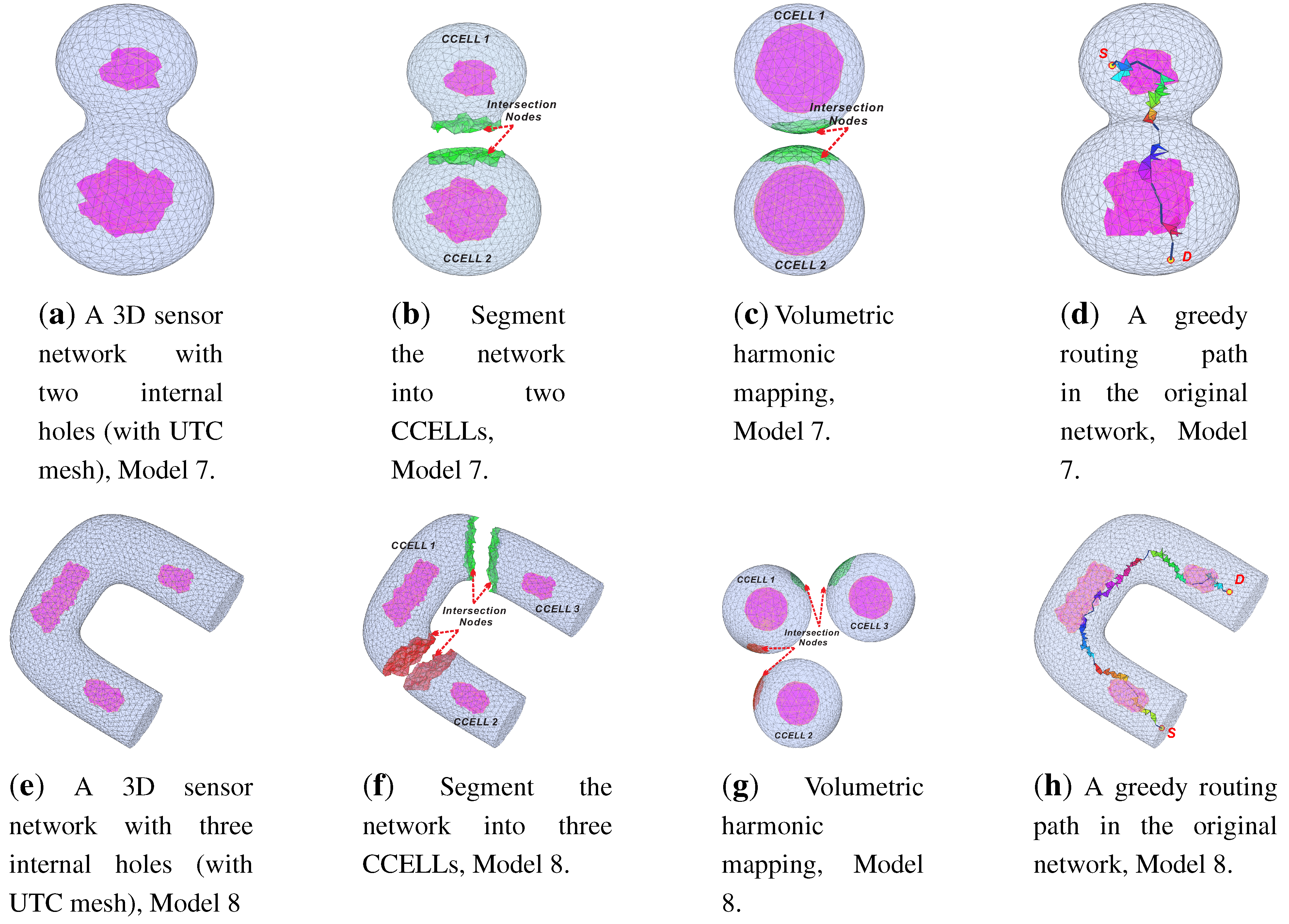
5.2. 3D Sensor Networks with Multiple Internal Holes

For a network with more than one inner hole, a clustering algorithm is adopted to segment the network into clusters. Each cluster centers at an inner hole, and contains one hole only. The same mapping algorithm discussed in Section 5.1 is then deployed for each cluster to generate virtual coordinates. Note here that the virtual coordinates of each clusters are independent of each other. “Aligning” the “cluster spheres” according to their positions in the original network is neither practical nor correct for global end-to-end greedy routing. For example, after the mapping, the network with two holes consists of two “cluster spheres”. Even we can align them according to their sharing nodes, the virtual coordinates obtained after the alignment do not guarantee the greedy end-to-end route across the two spheres (see Figure 7 for an example). Since global alignment is infeasible, routing across the clusters often relies on the “gateways” between adjacent clusters. However, it remains challenging to design such gateway-based routing under the constraints of constant-bounded storage and computation at individual nodes. To this end, we propose a tunnel-based routing scheme. It does not require global alignment and, at the same time, keeps the storage and computation cost on each node “nearly” a small constant. Moreover, it guarantees the global greedy end-to-end routing across the clusters and does not overload the gateway nodes like the traditional gateway scheme does. The proposed algorithm is outlined below.
Figure 7. Failure of end-to-end greedy routing after global alignment of two spheres of mapped CCELLs. The packet from S to D will be stuck at L m i n , which is closest to D in CCELL 1.
Axioms 03 00177 g007

5.2.1. Network Segmentation and Mapping

The first step is to segment a 3D sensor network with multiple inner holes into a set of clusters, each containing one hole only. We first give the definition of network segmentation and then introduce an algorithm to realize it.
Definition 13
Cluster cell (CCELL): Consider a 3D sensor network with m interior holes. Let { B i | 1 i m } denote the boundaries of the holes. The sensor network is decomposed into a set of sub-networks, or CCELLs, { C i | 1 i m } , as follows: C i = { q | | B i q | | B j q | , j i } , where | B i q | is the shortest hop distance from a node, q, to B i . Since the entire network is bounded, each CCELL is bounded, too. Therefore, the outer boundary of a CCELL forms a closed surface, denoted as Λ i .
To construct CCELLs, the exterior and interior boundaries of a sensor network can be extracted by identifying the boundary UTCs in a UTC mesh (see Section 2. An example of boundaries are illustrated in the first row of Figure 6 and Figure 8a,e, where the boundary nodes are highlighted in colors.
Based on Definition 13, CCELLs of a 3D sensor network can be established by an algorithm outlined below. Let B 0 denote the outer boundary and { B i | 1 i m } the inner boundaries. Each inner boundary node initiates a flooding message that includes its boundary ID and a hop counter that records the number of hops the message has traveled. A non-inner-boundary node learns its hop distance to nearby holes according to the received flooding messages. It always keeps the shortest distance and the corresponding boundary ID.
When flooding stops, a node checks the shortest distance(s) and the corresponding boundary ID(s) it has learned. If a non-inner-boundary node has equal shortest hop distance to at least two inner boundaries, B i and B j , the node is marked by selecting the one with the smaller ID, indicating that it belongs to corresponding CCELLs, i.e., Λ i if i < j , which is also called the intersection node. In the discrete case, the hop distances of a node to two inner boundaries are considered equal if they have the same hop counts or differ by one.
It is worth mentioning that under an extreme (artificial) condition, a CCELL established by the method introduced above may have more than one separate boundary (see [38] for a similar discussion on generalized Voronoi cells), where each boundary is still a closed surface. In such a case, an arbitrary boundary is chosen as CCELL.
Now, the 3D sensor network has been segmented into a set of CCELLs, and each CCELL is bounded by corresponding closed surface Λ i (see Figure 8b,f for example). For each CCELL, the same mapping algorithm discussed in Section 5.1 can be applied to build a local virtual coordinate system (see Figure 8c,g). Note here that the virtual coordinates of each CCELL are independent and not aligned with each other. Moreover, the intersection nodes will have at least one neighbor located in different CCELLs. Routing inside each CCELL is naturally supported, as we discussed in the network with one hole scenario. In the next part, we will propose a routing scheme, dubbed tunnel routing, to coordinate these local coordinates to support global routing across CCELLs.

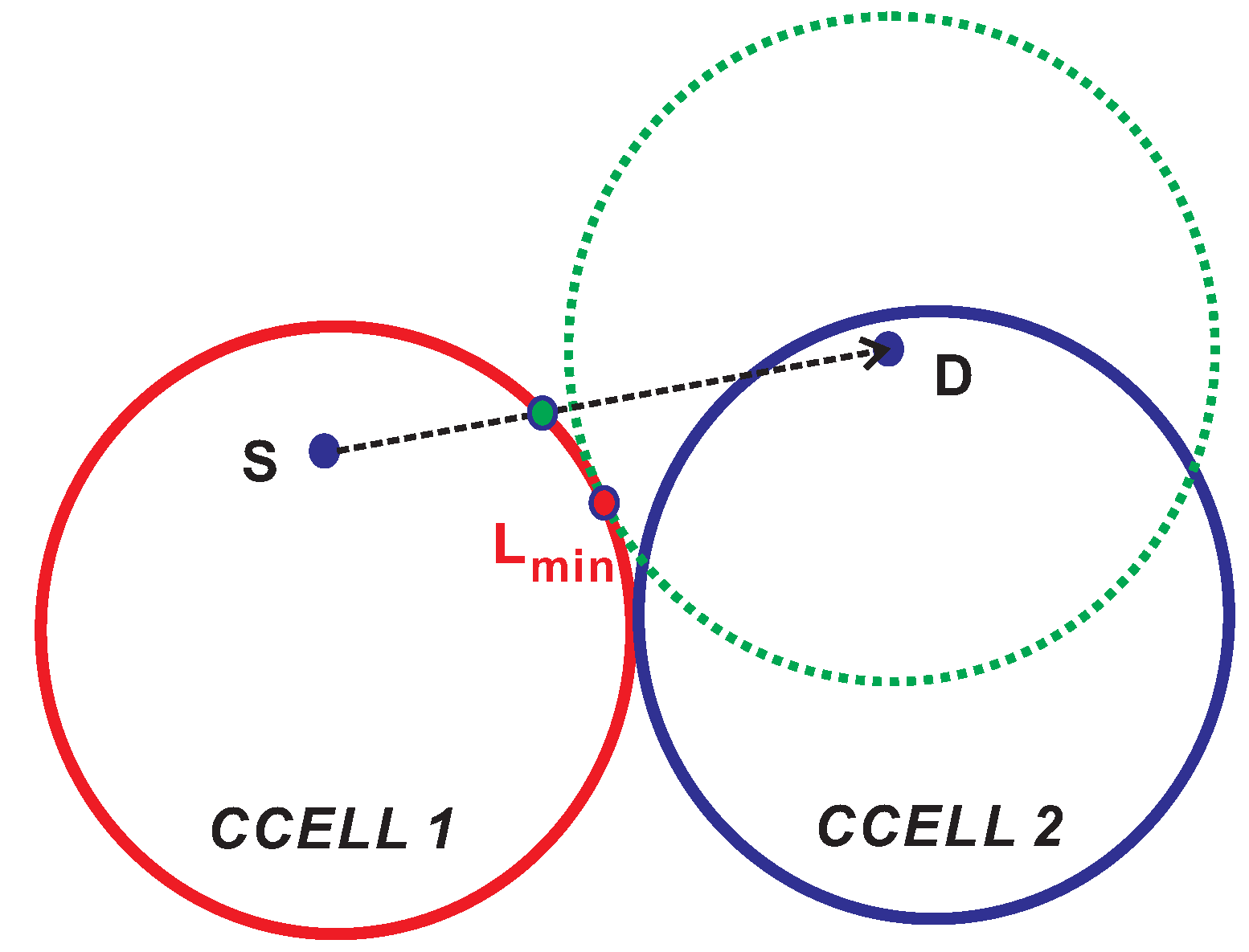
5.2.2. Tunnel Routing

The CCELLs constructed by network segmentation capture the approximated geometric shape of a 3D sensor network. A graph can make a compact representation of CCELLs available, where vertices represent CCELLs and an edge connects two vertices if the corresponding CCELLs are adjacent. Here, we say one CCELL is adjacent to the other, if at least one of its nodes has a neighbor belonging to the other CCELL. Let T i j indicate a tunnel from CCELL i to CCELL j, which is described by a point, t i j , and a radius, r i j , on the mapped spherical outer surface of CCELL i, where t i j is the “center” of intersection nodes (between CCELLs i and j), and r i j is the maximum radius of the circle centered at t i j containing only intersection nodes on the spherical surface of CCELL i (see Figure 9, for example). The information of T i j is broadcast to all the nodes within CCELL i. The message includes the tunnel description, t i j , r i j , and its adjacent CCELLs ID, j. Therefore, every node in the network can construct a global graph and, accordingly, establish a global routing table, which is very compact, with its size only proportional to the number of interior holes.
Figure 8. Illustration of the proposed greedy routing protocol for a network with multiple internal holes, Models 7 and 8 used in our simulations. (a,e) 3D sensor networks that have irregular outer and inner boundaries and have multiple internal holes. The nodes on the inner boundary are highlighted in purple. (b,f) After the segmentation, the networks are decomposed into cluster cells (CCELLs), each containing one hole only. The intersection nodes are highlighted in green and red. Additionally, we separate the CCELLs further apart for a clearer view. (c,g) The result after volumetric harmonic mapping, with both outer and inner boundaries mapped to spheres for each CCELL. The intersection nodes are in green and red, and here, we partially “align” the CCELLs to get a better view, but actually, the virtual coordinates of these CCELLs are independent of each other. (d,h) An example of the greedy routing path according to our proposed scheme is shown in the original network domain.
Axioms 03 00177 g008
Figure 9. Illustration of tunnel. Nodes in green area are the intersection nodes in CCELL i. t i j is the center of tunnel T i j . The area (on the spherical surface) enclosed by the yellow circle with radius r i j centered at t i j is tunnel T i j .
Axioms 03 00177 g009
If the source and destination are inside the same CCELL, routing in a CCELL (see Section 5.1) is applied. Otherwise, the source checks its global routing table to find the next hop CCELL and the tunnel to that CCELL. Then, the source randomly pick a target point, p i , on the spherical surface within the tunneland route toward p i . The algorithm of routing in a CCELL is employed to deliver the packet toward p i . Note that the packet is not necessary to actually reach p i . Since adjacent CCELLs share a good amount of intersection nodes, the packet can directly route to the next CCELL without passing through p i , as long as it meets an intersection node on the shared boundary. Thus, the traffic across CCELLs can be nicely distributed among the intersection node on the shared boundary between CCELLs. This has also been verified by our extensive simulations; see Section 6. The procedure repeats, until the packet enters the destination CCELL, where it can be delivered, as we have discussed in Section 5.1. Figure 8d visualizes the view of a global routing path where source S and destination D are located in different CCELLs. In addition, Figure 8d,h gives examples of end-to-end paths in a 3D network with two and three internal holes, respectively.
In summary, the proposed tunnel routing algorithm is a combination of greedy routing, face routing and conventional table-based routing with guaranteed delivery, reasonable path stretch and desired scalability. It decomposes a 3D sensor network with multiple holes into a set of CCELLs and maintains a small global routing table with a bounded size to route packets across CCELLs. The data delivery inside one CCELL is realized by greedy routing and face routing.
For each node involved in tunnel routing, the storage cost consists of two parts: a global routing table with the size, m (number of inner holes, which usually is a small constant for general 3D sensor networks), for routing across CCELLs and the virtual coordinates of its own and its neighbors (which is used by all greedy routing schemes and only related to the nodal degree) for routing in a CCELL. Thus, the storage cost of each node is nearly a constant, which provides great scalability to the network size.

6. Applications and Simulations

We have implemented the face-based greedy routing algorithm and the volumetric harmonic mapping (VHM) algorithm introduced above, in order to achieve highly efficient peer-to-peer greedy routing in 3D sensor networks. Moreover, we further apply the proposed routing algorithm in in-network data-centric storage and retrieval. The simulation results are presented below sequentially.

6.1. Peer-to-Peer Greedy Routing

Various 3D sensor networks of different sizes (ranging from 1,000 to 2,500) and shapes are simulated in this work. In addition to the network model shown in Figure 1 (Model 1) and Figure 8 (Model 7 and Model 8 with two and three internal holes), Figure 6 illustrates several other examples, where the first row shows original networks, the second row illustrates the established UTC mesh structures and the third row depicts the results after volumetric harmonic mapping. In all the models, sensor nodes are randomly distributed. The radio transmission range is around 0 . 11 , resulting in an average nodal degree between 16 to 30. Note that such a nodal degree is moderate in 3D, although it appears high for 2D networks. The boundaries are detected as discussed in the previous section. For example, the inner boundary is highlighted in magenta in Figure 6i,j.

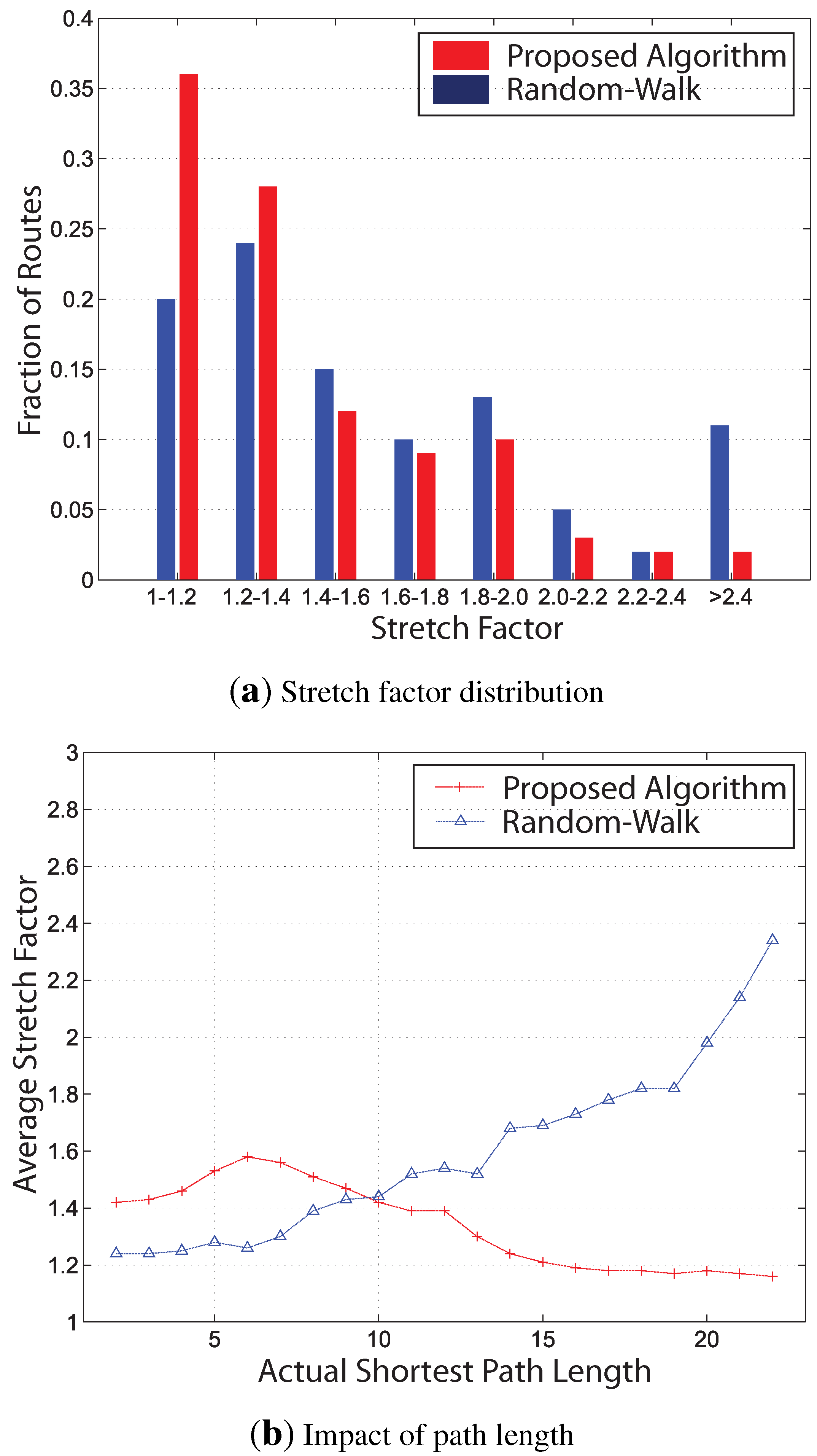
6.1.1. Stretch Factor

As proven in the previous sections, the proposed scheme guarantees successful data delivery between any pair of nodes. Therefore, we focus on the stretch factor in the performance evaluation. The stretch factor of a route is the ratio of the actual path length to the shortest path length. We randomly select 10,000 pairs of nodes to calculate the average stretch factor for each network model.
While many greedy routing algorithms have been proposed for wireless sensor networks, few of them can be applied in a 3D setting. Moreover, we only focus on truly greedy routing algorithms with constant-bounded storage and computation complexity in 3D sensor networks in this research. Therefore, random-walk [6] is the sole comparable scheme, as discussed in Section 1. Under random-walk, a packet is greedily advanced to its destination. If a local minimum is reached, it escapes from the local minimum by a random walk on a local spherical structure. Note that random-walk does not ensure deterministic routing results.
The average stretch factors of random-walk and our proposed algorithm are summarized in Table 1. As can be seen, the proposed scheme exhibits stable stretch factor and outperforms random-walk in all network models. In a contrast, the performance of random-walk heavily depends on the size of the hole and the shape of the network, experiencing a higher stretch factor under the network with a bigger hole (see Figure 6e Model 6 and Figure 8a Model 7) or heavy irregular network shapes (see Figure 8e Model 8).
Table 1. Comparison of stretch factors.
Model 1Model 2Model 3Model 4Model 5Model 6Model 7Model 8Average
Ours1.631.631.661.611.621.441.691.721.62
Random-walk [6]1.831.701.731.841.892.122.162.912.02
Figure 10 illustrates the distribution of the stretch factor based on Network Model 6. We observe that most routing paths under our proposed scheme have a low stretch factor. For example, 70% of routes have their stretch factor lower than 1 . 4 . On the other hand, the distribution under random-walk has a considerable shift to the right side. Particularly, there are about 20% of routes experiencing a stretch factor of 2 . 0 or higher (which means a routing path at least twice as long as the shortest path).
Figure 10. (a) More routes under the proposed scheme have low stretch factors than random-walk does; (b) with the increase of the actual path length between source and destination, the stretch factor decreases under our proposed scheme, while the stretch factor of random-walk grows noticeably.
Axioms 03 00177 g010
It is also an interesting observation from Figure 10b that, with the increase of the actual path length between source and destination, the stretch factor decreases under our proposed scheme. This is in sharp contrast to random-walk, where two far-separated nodes are likely located on the opposite side of the hole, and accordingly, conventional node-based greedy routing between them may fail, leading to a long random walk path.

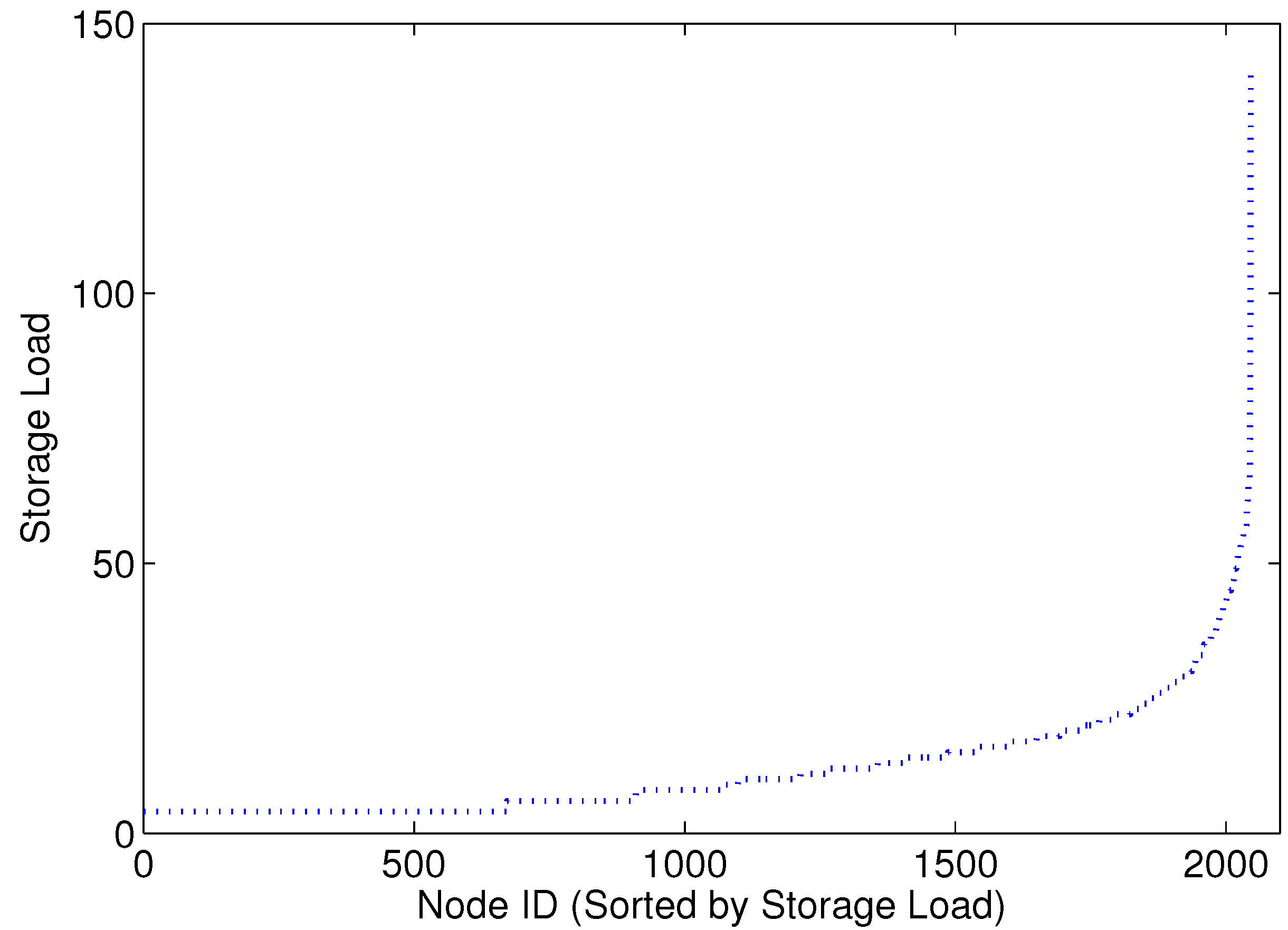
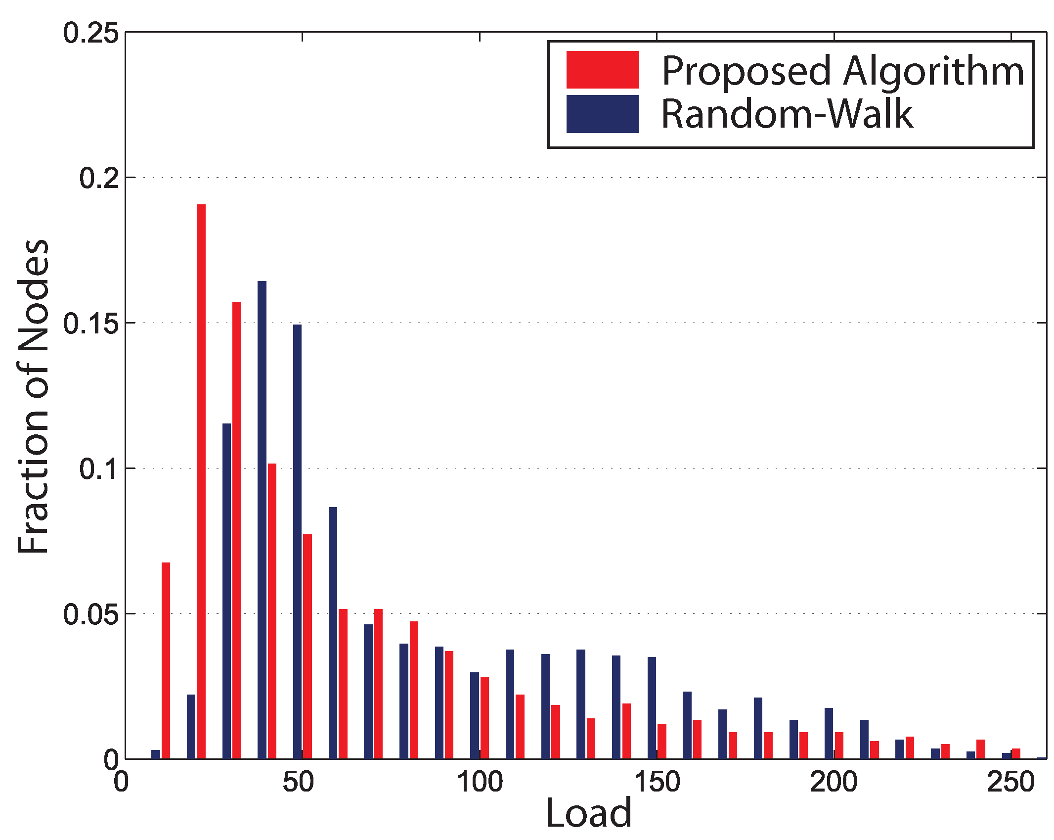
6.1.2. Load Distribution

We have also calculated the traffic load distribution among the sensor nodes, as illustrated in Figure 11. The traffic load under our proposed scheme is well balanced, with more than 40% of the nodes involved in less than 30 routes and around 60% in less than 50 routes. Random-walk performs greedy routing first and then randomly searches along the boundaries when a dead-end is reached. Thus, the nodes near boundaries (especially inner boundaries) usually experience heavy load.
Figure 11. Load distribution in routing.
Axioms 03 00177 g011

6.2. Data Storage and Retrieval

Our scheme guarantees greedy and stateless peer-to-peer routing in a 3D sensor network. Another possible application of the proposed scheme is for data centric networking, which supports in-network data storage and query. Traditionally, the underlying network used for data storage and retrieval needs to store a great amount of routing information. Let us consider a network without or with one internal hole first. With the proposed techniques, the whole network consists of tetrahedrons and is mapped into a unit sphere in a 3D space, which supports greedy peer-to-peer routing. Therefore, we propose to uniformly map a datum to a point inside of the unit sphere and let the tetrahedron, which contains the point to store the datum. Both data insertion and retrieval are naturally supported by greedy routing.

6.2.1. Where to Store the Data

Given a datum, finding the location to store it is the key issue in data-centric networking. To this end, we exploit the result of volumetric harmonic mapping, which maps the original network with an irregular shape to a ball. We adopt the polar coordinate system, where a point in a unit sphere can be represented by ( ρ , α , β ), where ρ is the distance from this point to the origin, α is the angle formed by the line connecting this point and the origin with the X-axis and β is the angle between the line and Y-axis. ρ is bounded to 0 ρ 1 for a network without a hole or r ρ 1 for a network with a hole, where r is the radius of the inner sphere in volumetric harmonic mapping.
First, we map a datum (possibly with multiple attributes) to a series of bits by using the method introduced in [39,40,41]. We select the ( 3 k + 1 )-th bits (where k ranges from zero to the largest value that depends on the length of the bit series) and concatenate them to a binary string, which is further normalized to yield ρ. Similarly, ( 3 k + 2 )-th and ( 3 k + 3 )-th bits are used to determine α and β, respectively. Since the unit ball (or hollow ball) is the volumetric harmonic mapping of the tetrahedron mesh of the original network, a point ( ρ , α , β ) must be within a tetrahedron. Thus, we simply select one of the four vertex of this tetrahedron to store the datum.

6.2.2. Route Data and Query

Once a datum is mapped to a point location ( ρ , α , β ), it is routed toward the location by following our proposed greedy routing algorithm. In each hop of routing, it checks if ( ρ , α , β ) is inside the current tetrahedron. If it is true, the routing terminates, and the datum is stored by one of the tetrahedron’s vertices that has the lowest load. Query and retrieval of data can be realized similarly. The data being queried is mapped to a point location, and the query is routed to the corresponding tetrahedron that contains the requested data.

6.2.3. Networks with Multiple Internal Holes

For networks with multiple internal holes, we can use a similar strategy as described in Section 5. First, we segment the network and apply VHM to map each CCELL into a spherical shell. Next, we modulus the mapped bits of a datum with m (the number of CCELLs of the network) to get i and assign this datum to CCELL i. Then, following the same procedure as discussed above, this datum is mapped into a point position within a spherical shell. According to the mapped position, the datum is routed by following our proposed greedy routing scheme in Section 5 to the target location and stored by one of the vertices of the tetrahedron containing this position. It is worth mentioning that the radius, r i , of the inner sphere of each CCELL i in VHM needs to be broadcast to all the nodes, while the radius of the outer spheres (which is one) is well known by all nodes.

6.2.4. Performance

We have carried out simulations to insert 10 , 000 data generated by a set of randomly chosen nodes for Model 1. Each datum has a value ranging from zero to 100. Figure 12 shows the distribution of the loading factor, i.e., the ratio of the actual load to the ideal load, where the ideal load is achieved when the data are evenly distributed over all nodes in the network. As can be seen, the loading factor is nicely distributed, where more than 40% of nodes enjoy a perfect loading factor of one, signifying well-balanced traffic among sensor nodes.
Figure 12. Distribution of the loading factor.
Axioms 03 00177 g012

7. Conclusions

Viewing significant challenges encountered in extending greedy routing from 2D to 3D space, we have investigated decentralized solutions to achieve greedy routing in 3D sensor networks. Our proposed approach is based on a unit tetrahedron cell (UTC) mesh structure. We have proposed a distributed algorithm to realize volumetric harmonic mapping of the UTC mesh under the spherical boundary condition. It is a one-to-one map that yields virtual coordinates for each node in the network. Since a boundary has been mapped to a sphere, node-based greedy routing is always successful thereon. At the same time, we have exploited the UTC mesh to develop a face-based greedy routing algorithm and proved its success at internal nodes. To route a data packet to its destination, face-based and node-based greedy routing algorithms are employed alternately at internal and boundary UTCs, respectively. For general networks with multiple internal holes, a segmentation and tunnel-based routing strategy is proposed on top of VHM to support global end-to-end routing. To our best knowledge, this is the first work that realizes truly deterministic routing with constant-bounded storage and computation in general 3D wireless sensor networks.

Acknowledgments

Hongyi Wu is partially supported by NSF CNS-1018306 and CNS-1320931. Miao Jin is partially supported by NSF CCF-1054996, CNS-1018306 and CNS-1320931. Xiaotian Yin and Xianfeng David Gu are partially supported by NSF CNS-1016829.

Author Contributions

We proposed a decentralized solution to achieve greedy routing with guaranteed delivery in 3D sensor networks. To our best knowledge, this is the first work that realizes truly deterministic routing with constant-bounded storage and computation in general 3D wireless sensor networks.

Conflicts of Interest

The authors declare no conflict of interest.

References

  1. Bai, X.; Zhang, C.; Xuan, D.; Teng, J.; Jia, W. Low-connectivity and full-coverage three dimensional networks. In Proceedings of the MobiHOC, New Orleans, LA, USA, 18–21 May 2009; pp. 145–154.
  2. Bai, X.; Zhang, C.; Xuan, D.; Jia, W. Full-coverage and K-connectivity (K = 14, 6) three dimensional networks. In Proceedings of the INFOCOM, Rio de Janeiro, Brazil, 19–25 April 2009; pp. 388–396.
  3. Liu, C.; Wu, J. Efficient geometric routing in three dimensional ad hoc networks. In Proceedings of INFOCOM, Rio de Janeiro, Brazil, 19–25 April 2009; pp. 2751–2755.
  4. Kao, T.F.G.; Opatmy, J. Position-based routing on 3D geometric graphs in mobile ad hoc networks. In Proceedings of the 17th Canadian Conference on Computational Geometry, Windsor, ON, Canada, 10–12 August 2005; pp. 88–91.
  5. Opatrny, J.; Abdallah, A.; Fevens, T. Randomized 3D position-based routing algorithms for ad-hoc networks. In Proceedings of the Third Annual International Conference on Mobile and Ubiquitous Systems: Networking & Services, San Jose, CA, USA, July 2006; pp. 1–8.
  6. Flury, R.; Wattenhofer, R. Randomized 3D geographic routing. In Proceedings of the INFOCOM, Phoenix, AZ, USA, 13–18 April 2008; pp. 834–842.
  7. Li, F.; Chen, S.; Wang, Y.; Chen, J. Load balancing routing in three dimensional wireless networks. In Proceedings of the ICC, Beijing, China, 19–23 May 2008; pp. 3073–3077.
  8. Zhou, J.; Chen, Y.; Leong, B.; Sundar, P. Practical 3D geographic routing for wireless sensor networks. In Proceedings of the SenSys, Zurich, Switzerland, 3–5 November 2010; pp. 337–350.
  9. Pompili, D.; Melodia, T.; Akyildiz, I.F. Routing algorithms for delay-insensitive and delay-sensitive applications in underwater sensor networks. In Proceedings of the MobiCom, Los Angeles, CA, USA, 23–29 September 2006; pp. 298–309.
  10. Cheng, W.; Teymorian, A.Y.; Ma, L.; Cheng, X.; Lu, X.; Lu, Z. Underwater Localization in Sparse 3D Acoustic Sensor Networks. In Proceedings of the INFOCOM, Phoenix, AZ, USA, 13–18 April 2008; pp. 798–806.
  11. Allred, J.; Hasan, A.B.; Panichsakul, S.; Pisano, W.; Gray, P.; Huang, J.; Han, R.; Lawrence, D.; Mohseni, K. SensorFlock: An airborne wireless sensor network of micro-air vehicles. In Proceedings of the SenSys, Sydney, NSW, Australia, 6–9 November 2007; pp. 117–129.
  12. Cui, J.H.; Kong, J.; Gerla, M.; Zhou, S. Challenges: Building scalable mobile underwater wireless sensor networks for aquatic applications. IEEE Netw. 2006, 20, 12–18. [Google Scholar]
  13. Bose, P.; Morin, P.; Stojmenovic, I.; Urrutia, J. Routing with guaranteed delivery in ad hoc wireless networks. In Proceedings of the Third Workshop Discrete Algorithms and Methods for Mobile Computing and Communications, Seattle, WA, USA, 20 August 1999; pp. 48–55.
  14. Karp, B.; Kung, H. GPSR: Greedy perimeter stateless routing for wireless networks. In Proceedings of the MobiCom, Rome, Italy, 16–21 July 2001; pp. 1–12.
  15. Kranakis, E.; Singh, H.; Urrutia, J. Compass routing on geometric networks. In Proceedings of the Canadian Conference on Computational Geometry (CCCG), Vancouver, BC, Canada, 15–18 August 1999; pp. 51–54.
  16. Kuhn, F.; Wattenhofer, R.; Zhang, Y.; Zollinger, A. Geometric ad-hoc routing: Theory and practice. In Proceedings of the 22nd ACM Symposium on the Principles of Distributed Computing, Boston, MA, USA, 13–16 July 2003; pp. 63–72.
  17. Kuhn, F.; Wattenhofer, R.; Zollinger, A. Worst-case optimal and average-case efficient geometric ad-hoc routing. In Proceedings of the MobiHOC, Annapolis, MD, USA, 1–3 June 2003; pp. 267–278.
  18. Mitra, B.L.S.; Liskov, B. Path vector face routing: Geographic routing with local face information. In Proceedings of the ICNP, Boston, MA, USA, 6–9 November 2005; pp. 147–158.
  19. Frey, H.; Stojmenovic, I. On delivery guarantees of face and combined greedy-face routing in ad hoc and sensor networks. In Proceedings of the MobiCom, Los Angeles, CA, USA, 23–29 September 2006; pp. 390–401.
  20. Tan, G.; Bertier, M.; Kermarrec, A.M. Visibility-graph-based shortest-path geographic routing in sensor networks. In Proceedings of the INFOCOM, Rio de Janeiro, Brazil, 19–25 April 2009; pp. 1719–1727.
  21. Papadimitriou, C.; Ratajczak, D. On a conjecture related to geometric routing. Theor. Comput. Sci. 2005, 344, 3–14. [Google Scholar] [CrossRef]
  22. Angelini, P.; Frati, F.; Grilli, L. An algorithm to construct greedy drawings of triangulations. In Proceedings of the 16th International Symposium on Graph Drawing, Heraklion, Crete, Greece, 21–24 September 2008; pp. 26–37.
  23. Leighton, T.; Moitra, A. Some results on greedy embeddings in metric spaces. In Proceedings of the 49th IEEE Annual Symposium on Foundations of Computer Science, Philadelphia, PA, USA, 25–28 October 2008; pp. 337–346.
  24. Kleinberg, R. Geographic routing using hyperbolic space. In Proceedings of the INFOCOM, Anchorage, AK, USA, 6–12 May 2007; pp. 1902–1909.
  25. Cvetkovski, A.; Crovella, M. Hyperbolic embedding and routing for dynamic graphs. In Proceedings of the INFOCOM, Rio de Janeiro, Brazil, 19–25 April 2009; pp. 1647–1655.
  26. Sarkar, R.; Yin, X.; Gao, J.; Luo, F.; Gu, X.D. Greedy routing with guaranteed delivery using ricci flows. In Proceedings of the IPSN, San Francisco, CA, USA, 13–16 April 2009; pp. 121–132.
  27. Flury, R.; Pemmaraju, S.; Wattenhofer, R. Greedy routing with bounded stretch. In Proceedings of the INFOCOM, Rio de Janeiro, Brazil, 19–25 April 2009; pp. 1737–1745.
  28. Durocher, S.; Kirkpatrick, D.; Narayanan, L. On routing with guaranteed delivery in three-dimensional ad hoc wireless networks. In Proceedings of the International Conference on Distributed Computing and Networking, Kolkata, India, 5–8 January 2008; pp. 546–557.
  29. Zhou, H.; Xia, S.; Jin, M.; Wu, H. Localized algorithm for precise boundary detection in 3D wireless networks. In Proceedings of the ICDCS, Genoa, Italy, 21–25 July 2010; pp. 744–753.
  30. Zhong, Z.; He, T. MSP: Multi-sequence positioning of wireless sensor nodes. In Proceedings of the SenSys, Sydney, NSW, Australia, 6–9 November 2007; pp. 15–28.
  31. Giorgetti, G.; Gupta, S.; Manes, G. Wireless localization using self-organizing maps. In Proceedings of the IPSN, Cambridge, MA, USA, 25–27 April 2007; pp. 293–302.
  32. Li, L.; Kunz, T. Localization applying an efficient neural network mapping. In Proceedings of the Int’l Conference on Autonomic Computing and Communication Systems, Rome, Italy, 28–30 October 2007; pp. 1–9.
  33. Shang, Y.; Ruml, W.; Zhang, Y.; Fromherz, M.P.J. Localization from mere connectivity. In Proceedings of the MobiHOC, Annapolis, MD, USA, 1–3 June 2003; pp. 201–212.
  34. Shang, Y.; Ruml, W. Improved MDS-based localization. In Proceedings of the INFOCOM, Hong Kong, China, 7–11 March 2004; pp. 2640–2651.
  35. Gu, X.; Wang, Y.; Yau, S.T. Volumetric harmonic map. Commun. Inf. Syst. 2003, 3, 191–202. [Google Scholar] [CrossRef]
  36. Wan, S.; Ye, T.; Li, M.; Zhang, H.; Li, X. Efficient spherical parametrization using progressive optimization. In Proceedings of the First International Conference on Computational Visual Media, Beijing, China, 8–10 November 2012; pp. 170–177.
  37. Gu, X.; Wang, Y.; Chan, T.F.; Thompson, P.M.; Yau, S.T. Genus zero surface conformal mapping and its application to brain surface mapping. IEEE Tran. Med. Imaging 2004, 23, 949–958. [Google Scholar] [CrossRef] [PubMed]
  38. Alt, H.; Schwarzkopf, O. The voronoi diagram of curved objects. In Proceedings of the 11th Annual Symposium on Computational Geometry, Vancouver, BC, Canada, 5–7 June 1995; pp. 89–97.
  39. Li, J.; Jannotti, J.; de Couto, D.S.J.; Karger, D.R.; Morris, R. A scalable location service for geographic ad hoc routing. In Proceedings of the MobiCom, Boston, MA, USA, 6–11 August 2000; pp. 120–130.
  40. Li, X.; Kim, Y.J.; Govindan, R.; Hong, W. Multi-dimensional range queries in sensor networks. In Proceedings of the SenSys, Los Angeles, CA, USA, 5–7 November 2003; pp. 63–75.
  41. Yu-Chi, C.; I-Fang, S.; Chiang, L. Supporting multi-dimensional range query for sensor networks. In Proceedings of the ICDCS, Toronto, ON, Canada, 25–29 June 2007; pp. 35–35.

