Indoor Temperature Validation of Low-Income Detached Dwellings under Tropical Weather Conditions

 ,
,
Abstract
:1. Introduction
2. Literature Review
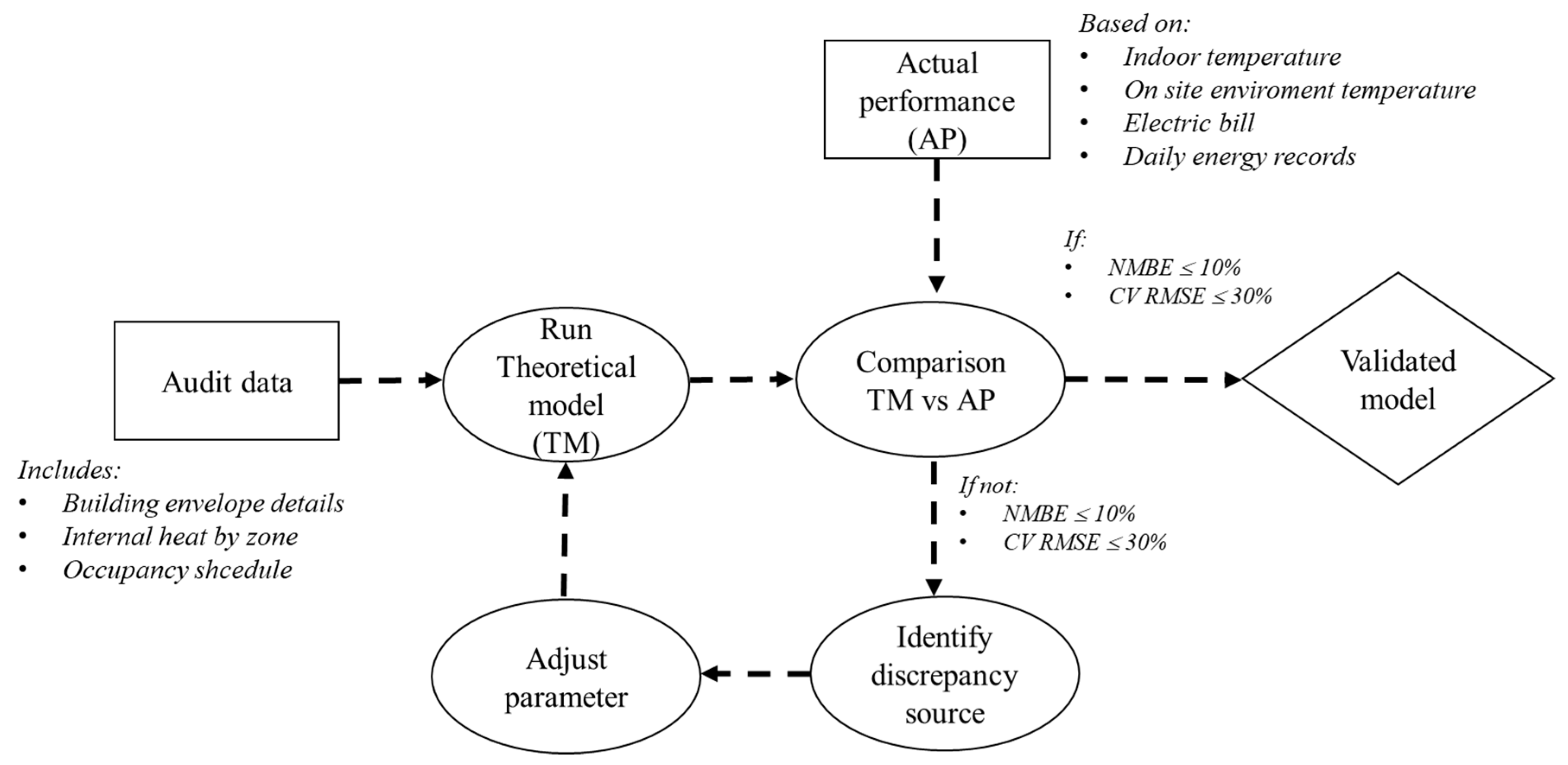
3. Methodology
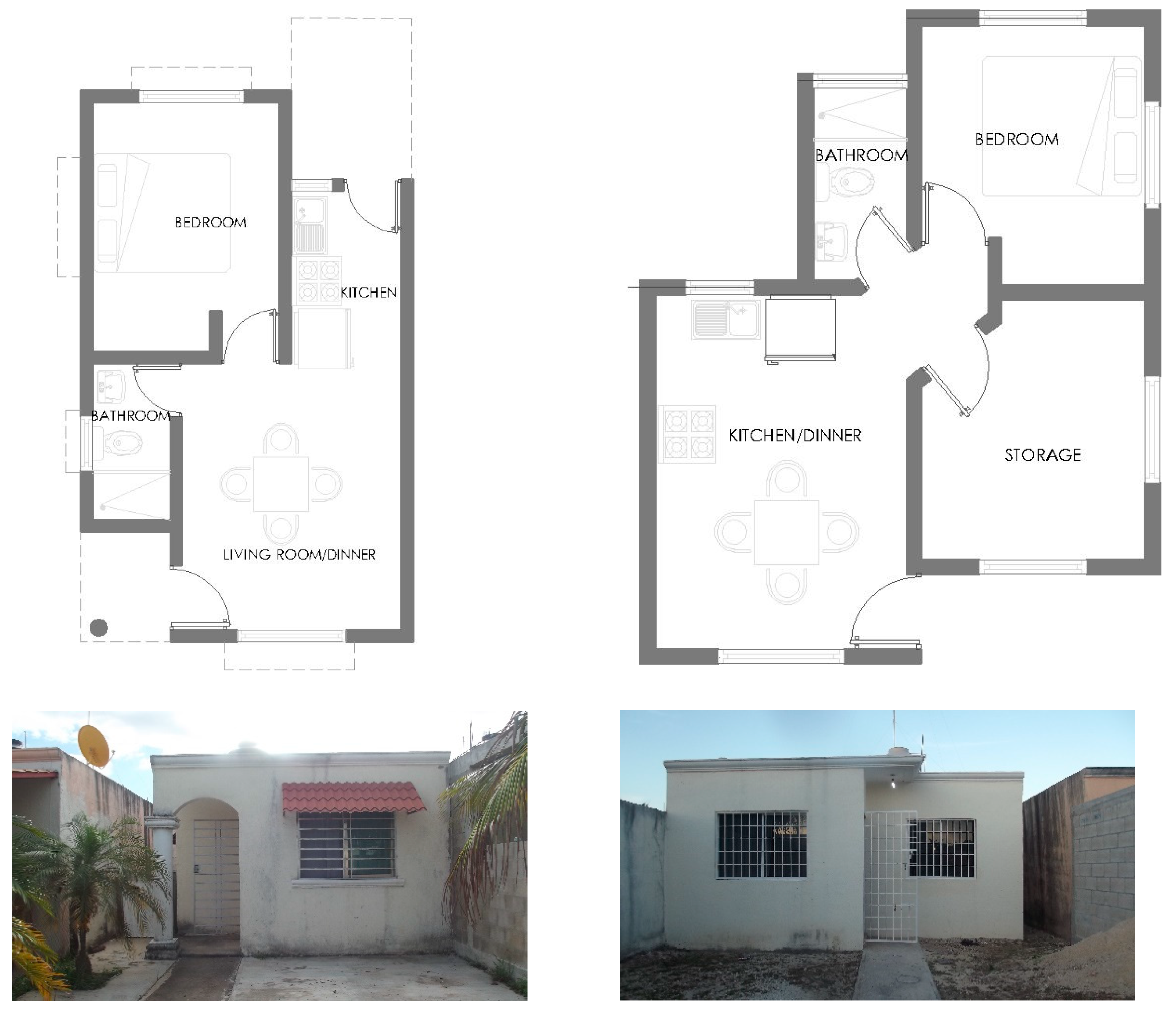
3.1. Case Studies
3.2. Equipment and Data Recording
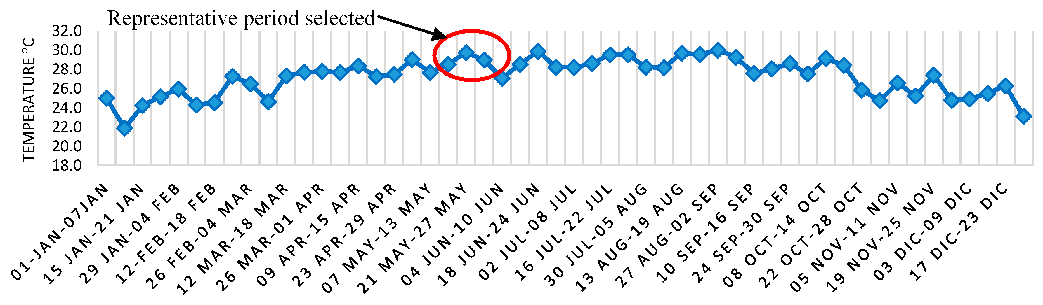
4. Results and Discussion
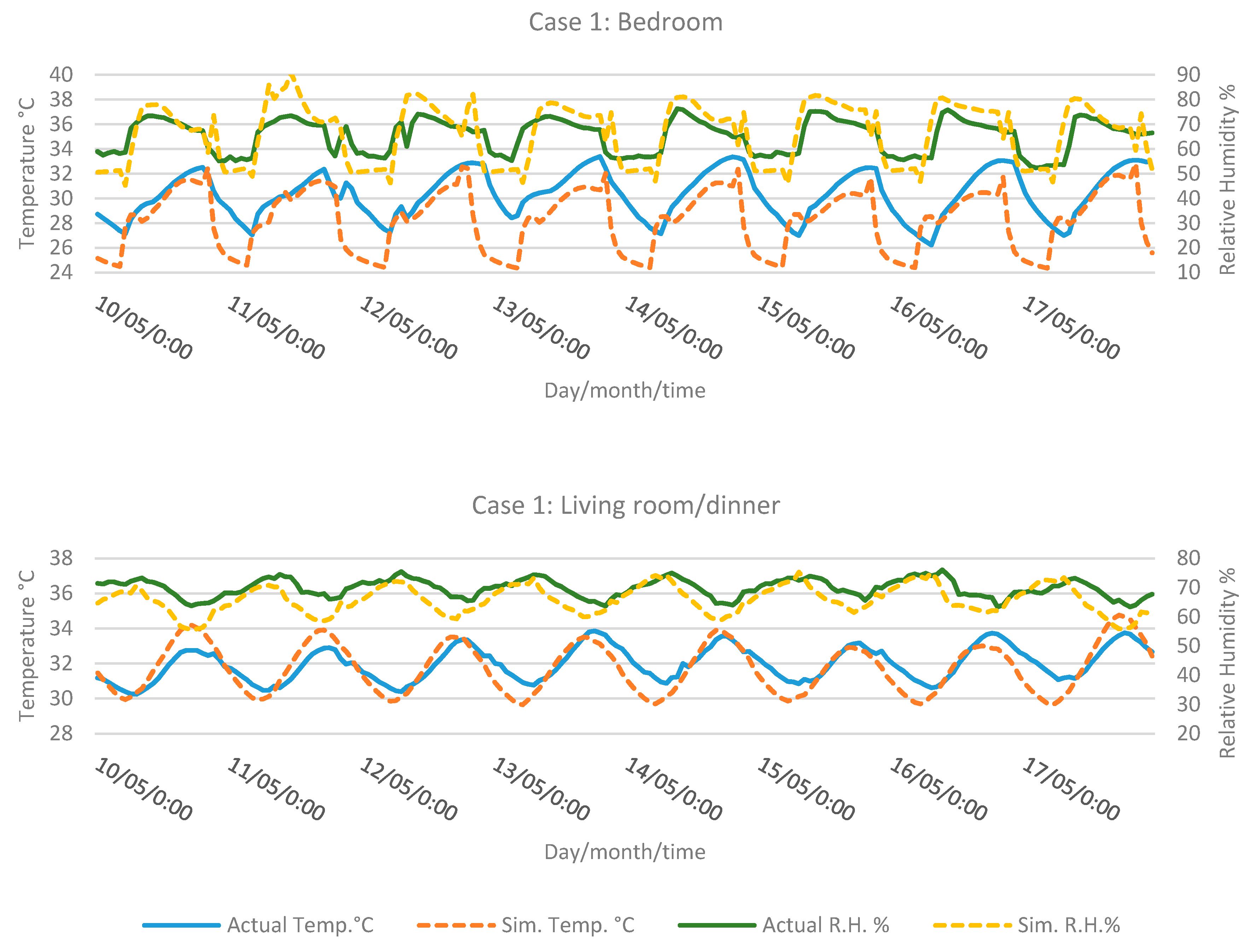
4.1. First Evaluation
4.2. Second Evaluation
4.3. Indoor Temperature Model Calibration
5. Conclusions
Author Contributions
Acknowledgments
Conflicts of Interest
References
- National Institute of Statistics and Geography. Intercensal Survey 2015; INEGI: Aguascalientes, Mexico, 2015.
- Cerón-Palma, I.; Sanyé-Mengual, E.; Oliver-Solá, J.; Montero, J.I.; Ponce-Caballero, C.; Rieradevall, J. Towards a green sustainable strategy for social neighbourhoods in Latin America: Case from social housing in Merida, Yucatan, Mexico. Habitat Int. 2013, 38, 47–56. [Google Scholar]
- OECD. OECD Urban Policy Reviews: Mexico 2015 Transforming Urban Policy and Housing; OECD Publishing: Paris, Finance, 2015. [Google Scholar]
- Aguilar, G.A.; Santos, C. Informal settlements’ needs and enviromental conservation in Mexico City: An unsolved challenge land use-policy. Land Use Policy 2011, 4, 649–662. [Google Scholar] [CrossRef]
- Taha, H.; Akbari, H.; Rosenfeld, A.; Huang, J. Residential cooling loads and the urban heat Island- the effects of albedo. Build. Environ. 1988, 24, 271–283. [Google Scholar] [CrossRef]
- Fox, J.; Osmond, P. The effect of building facades on outdoor microclimate -reflectance recovery from terrestrial multispectral images using a robust empirical line method. Climate 2018, 6, 56. [Google Scholar] [CrossRef]
- Oropeza-Pérez, I.; Ostergaard, P.A. Energy Saving Potential of Utilizing Natural Ventilation Under Warm Conditions- A case study of México. Appl. Enegy 2014, 130, 20–32. [Google Scholar] [CrossRef]
- Oropeza-Pérez, I. Comparative economic assessment of the energy performance of air-conditioning within the Mexican residential sector. Energy Rep. 2016, 2, 147–154. [Google Scholar] [CrossRef] [Green Version]
- GIZ/INFONAVIT. Study of Optimization of Energy Efficiency in Low-Income Housing; INFONAVIT: Mexico City, Mexico, 2011. [Google Scholar]
- Tisov, A.; Siroky, J.; Kolarik, J. Key figures for joint assesment of indoor enviromental quality (IEQ) and energy consumption in modern buildings—A literature review. In Proceedings of the 12th REHVA World Congress, Aalborg, Denmark, 22–25 May 2016. [Google Scholar]
- De Wilde, P. The gap between predicted and measured energy performance of buildings: A framework for investigation. Autom. Constr. 2014, 41, 40–49. [Google Scholar] [CrossRef]
- Shi, X.; Si, B.H.; Zhao, J.S.; Tian, Z.C.; Wang, C.; Jin, X.; Zhou, X. Magnitude, causes, and solutions of the performance gap of buildings: A review. Sustainability 2018, 11, 937. [Google Scholar] [CrossRef]
- Mustafaraj, G.; Marini, D.; Costa, A.; Keane, M. Model calibration for building energy efficiency simulation. Appl. Energy 2014, 130, 72–85. [Google Scholar] [CrossRef]
- Royapoor, M.; Roskilly, T. Building model calibration using energy and enviromental data. Energy Build. 2015, 94, 109–120. [Google Scholar] [CrossRef]
- Mohegh, A.; Levison, R.; Taha, H.; Gilbert, H.; Zhang, J.; Li, Y.; Tang, T.; Ban-Weiss, G.A. Observational evidence of neighborhood scale reductions in air temperature assosiated with increases in roof albedo. Climate 2018, 6, 98. [Google Scholar] [CrossRef]
- Amorim, M.C.C.T.; Dubreuil, V. Intensity of Urban Heat Islands in tropical and temperate climates. Climate 2017, 5, 91. [Google Scholar] [CrossRef]
- ASHRAE Inc. ASHRAE Guideline 14-2002: Measurement of Energy and Demand Savings; ASHRAE: Atlanta, GA, USA, 2002. [Google Scholar]
- Eguía Oller, P.; Alonso Rodríguez, J.M.; Saavedra González, Á.; Arce Fariña, E.; Granada Álvarez, E. Improving the Calibration of Building Simulation with Interpolated Weather Datasets. Renew. Energy 2018, 122, 608–618. [Google Scholar] [CrossRef]
- Paliouras, P.; Matzaflaras, N.; Peuhkuri, R.H.; Kolarik, J. Using indoor enviroment parameters for calibration of building simulation model—A passive house case study. Energy Procedia 2015, 78, 1227–1232. [Google Scholar] [CrossRef]
- Roberti, F.; Oberegger, U.F.; Gasparella, A. Calibrating historic building energy models to hourly indoor air and surface temperaures: Methodology and case study. Energy Build. 2015, 108, 236–243. [Google Scholar] [CrossRef]
- Cárdenas, J.; Osma, G.; Merchian, A.; Ordoñez, G. Characterization of Enviromental and Energy Performance of an Average Social Dwelling in a Tropical Region of Colombia. WIT Trans. Ecol. Environ. 2016, 204, 859–870. [Google Scholar]
- Miño-Rodriguez, I.; Naranjo-Mendoza, C.; Korolija, I. Thermal assesment of low-cost rural housing—A case of study in the Ecuadorian Andes. Buildings 2016, 6, 36. [Google Scholar] [CrossRef]
- García, Y.; Cuadrado, J.; Blanco, J.M.; Roji, E. Optimizing the indoor thermal behavoiur of housing units in hot humid climates: Analysis and modelling of sustainable constructive alternatives. Indoor Built Environ. 2018, 1–19. [Google Scholar] [CrossRef]
- Cho, K.H.; Kim, S.S. Energy performance assesment acording to data acquisition levels of existing buildings. Energies 2019, 12, 1149. [Google Scholar] [CrossRef]
- Ruíz, G.R.; Bandera, C.F. Validation of calibrated energy models: Common errors. Energies 2017, 10, 1587. [Google Scholar] [CrossRef]
- Municipality of Othón P. Blanco. Urban Development Program of Othón P. Blanco, Quintana Roo; Municipality of Othón P. Blanco: Chetumal, Mexico, 2018. [Google Scholar]
- García, E. Modification to Köppen’s System Classification; UNAM: Mexico City, Mexico, 2004. [Google Scholar]
- National Institute of Statistics and Geography. Statistical and Geographyc Yearbook of Quintana Roo 2017; INEGI: Aguascalientes, Mexico, 2017.
- EnergyPlusTM. Enineering Reference. The Refernce to EnergyPlus Calculations. 2015. Available online: https://energyplus.net/sites/default/files/pdfs_v8.3.0/EngineeringReference.pdf (accessed on 20 April 2019).
- Secretary of Energy. Mexican Official Standard NOM-026-ENER-2015, Energy Efficiency in Split Type Air Conditioners with Variable Refrigerant Flow, Free Discharge and without Air Constrictors.Boundaries, Testing and Labeling Methods; SENER: Mexico City, Mexico, 2015. [Google Scholar]
- American Society of Heating. Refrigerating and Air-Conditioning Engineers, ASHRAE Handbook Fundamentals SI; ASHRAE: Atlanta, GA, USA, 2009. [Google Scholar]
- ASHRAE. ANSI/ASHRAE Standard 55-2017: Thermal Environmental Conditions for Human Occupancy; ASHRAE: Atlanta, GA, USA, 2017. [Google Scholar]
- Enriquez, R.; Jímenez, M.J.; Heras, M.R. Towards non-intrusive thermal load monitoring of buildings: BES calibration. Appl. Energy 2017, 191, 44–54. [Google Scholar] [CrossRef]
- Association of the Air Tightness Testing & Measurement. ATTMA Technical Starndards L1 Measuring Air Permeability of Building Envelopes (Dwellings); British Institute of Non-Destructive Testing: Northampton, UK, 2010. [Google Scholar]
- Ratner, B. The correlation coefficient: Its values range between +1/-1, or do they? J. Target. Meas. Anal. Mark. 2009, 17, 139–142. [Google Scholar] [CrossRef]
- Eleftheriadis, G.; Hamdy, M. The impact of insulation and HVAC degradation on overallbuilding energy performance: A case study. Buildings 2018, 8, 23. [Google Scholar] [CrossRef]


| UHI | Urban Heat Island |
| NAMA | National Appropiate Mitigation Actions |
| EER | Energy Efficiency Ratio |
| NMBE | Nominal Mean Bias Error |
| CV(RMSE) | Coefficient of Variation of the Root Mean Square Error |
| ASHRAE | American Society of Heating, Refrigerating and Air-Conditioning Engineers |
| U-value | Thermal Transmittance |
| Case 1 | Case 2 | |
|---|---|---|
| Orientation | Northeast | Southwest |
| Total Ocupancy | 2 | 2 |
| Area (m²) | 35.45 | 42.5 |
| Zones | Living room/dinner | Kitchen/dinner |
| Air conditioning Capacity kW | Kitchen | Bathroom |
| Bathroom | Bedroom(storage) | |
| Bedroom | Main bedroom | |
| 1.85 | 1.30 | |
| Energy efficiency ratio | 4.10 | 3.52 |
| Envelope element | Characteristics | U-value (W/m²K) | Case 1 | Case 2 |
|---|---|---|---|---|
| Floor | 100 mm concrete slab | 4.73 | YES | YES |
| External/Inter-nal walls | 15mm exterior mortar, 150 mm concrete hollow block, 15 mm interior mortar | 2.66 | YES | YES |
| Roof | 30mm concrete slab, 150 mm joist and concrete hollow brick, 15 mm interior mortar | 3.377 | YES | YES |
| Glazing | Absorbent green 6 mm | 5.808 | YES | NO |
| Absorbent grey 6 mm | 5.812 | NO | YES | |
| Window awning | 1.5 mm galvanized steel sheet | 8.33 | YES | NO |
| TEMPERATURE | RELATIVE HUMIDITY | ENERGY CONSUMPTION kW | |||||||||
|---|---|---|---|---|---|---|---|---|---|---|---|
| Mean A. °C | Mean S. °C | NMBE% | CV RMSE% | Mean A. % | Mean S. % | NMBE% | CV RMSE% | AP | TM | % ERROR | |
| Case 1 | 28.63 | 26.66 | 6.89 | 10.85 | 63.13 | 65.29 | −3.43 | 20.58 | 711.70 | 754.39 | −5.99 |
| Case 2 | 25.74 | 27.12 | −5.36 | 10.48 | 53.14 | 64.41 | −21.20 | 33.66 | 202.60 | 541.41 | −167.18 |
| Temperature °C | Relative Humidity % | ||||||
|---|---|---|---|---|---|---|---|
| MIN. WEEK | MAX. WEEK | MEAN | MIN. WEEK | MAX. WEEK | MEAN | ||
| Case 1 | Macro- environment | 27.40 | 32.30 | 29.54 | 67.00 | 88.00 | 78.65 |
| Micro-environment | 26.77 | 37.54 | 30.16 | 55.01 | 85.95 | 73.46 | |
| Case 2 | Macro- environment | 25.10 | 33.70 | 29.55 | 50.00 | 92.00 | 73.98 |
| Micro-environment | 25.31 | 40.67 | 31.03 | 36.89 | 85.10 | 65.91 | |
| Temperature | Relative Humidity | |||||||||
|---|---|---|---|---|---|---|---|---|---|---|
| R² | MEAN °C | NMBE% | CV (RMSE)% | R² | MEAN % | NMBE% | CV (RMSE) % | |||
| Case 1 | Bedroom | ITER. 1 | 0.25 | 26.11 | 16.03 | 18.17 | 0.41 | 60.85 | 7.26 | 13.25 |
| ITER. Op. | 0.37 | 28.29 | 7.10 | 16.72 | 0.68 | 66.52 | −1.88 | 11.27 | ||
| Living room | ITER. 1 | 0.67 | 28.41 | 12.57 | 12.97 | 0.36 | 74.86 | −6.79 | 10.70 | |
| ITER. Op. | 0.68 | 31.76 | 0.68 | 2.62 | 0.64 | 65.85 | 5.96 | 7.44 | ||
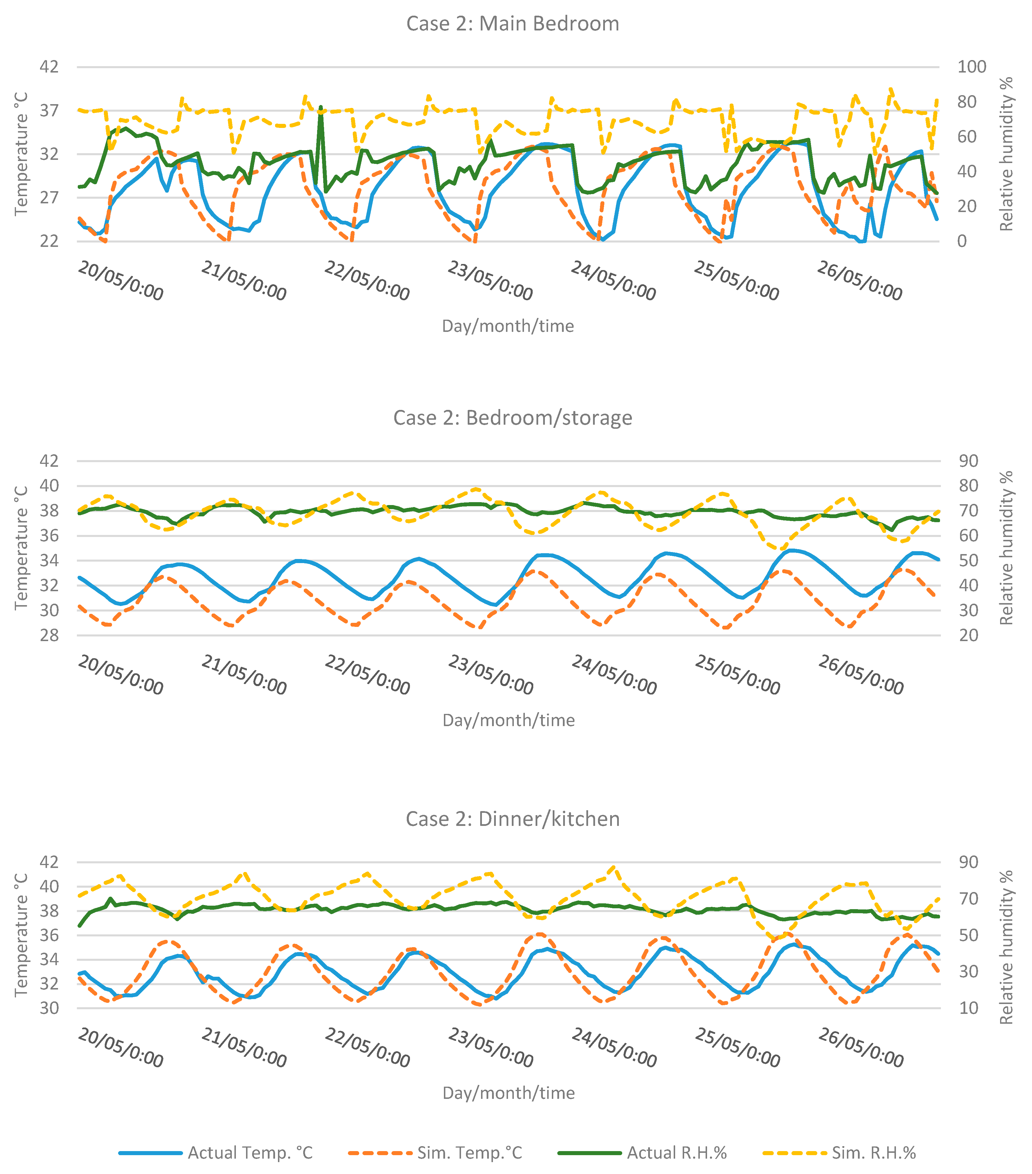
| Case 2 | Main Bedroom | ITER. 1 | 0.09 | 29.35 | −5.01 | 13.77 | 0.06 | 63.86 | −29.58 | 38.51 |
| ITER. Op. | 0.38 | 28.09 | −0.74 | 11.01 | 0.05 | 69.20 | −35.01 | 40.49 | ||
| Dinner/ kitchen | ITER. 1 | 0.54 | 31.16 | 5.73 | 6.95 | 0.40 | 64.27 | −9.55 | 14.72 | |
| ITER. Op. | 0.62 | 32.94 | 0.02 | 3.42 | 0.43 | 70.58 | −8.94 | 13.24 | ||
| Bedroom (storage) | ITER. 1 | 0.47 | 30.27 | 7.92 | 8.70 | 0.43 | 73.14 | −4.86 | 9.79 | |
| ITER. Op. | 0.51 | 30.80 | 6.07 | 6.87 | 0.44 | 68.97 | 0.88 | 6.39 | ||
© 2019 by the authors. Licensee MDPI, Basel, Switzerland. This article is an open access article distributed under the terms and conditions of the Creative Commons Attribution (CC BY) license (http://creativecommons.org/licenses/by/4.0/).
Share and Cite
Barrientos-González, R.A.; Vega-Azamar, R.E.; Cruz-Argüello, J.C.; Oropeza-García, N.A.; Chan-Juárez, M.; Trejo-Arroyo, D.L. Indoor Temperature Validation of Low-Income Detached Dwellings under Tropical Weather Conditions. Climate 2019, 7, 96. https://doi.org/10.3390/cli7080096
Barrientos-González RA, Vega-Azamar RE, Cruz-Argüello JC, Oropeza-García NA, Chan-Juárez M, Trejo-Arroyo DL. Indoor Temperature Validation of Low-Income Detached Dwellings under Tropical Weather Conditions. Climate. 2019; 7(8):96. https://doi.org/10.3390/cli7080096
Chicago/Turabian StyleBarrientos-González, R. Alexis, Ricardo E. Vega-Azamar, Julio C. Cruz-Argüello, Norma A. Oropeza-García, Maritza Chan-Juárez, and Danna L. Trejo-Arroyo. 2019. "Indoor Temperature Validation of Low-Income Detached Dwellings under Tropical Weather Conditions" Climate 7, no. 8: 96. https://doi.org/10.3390/cli7080096