Effect of the Variable Viscosity on the Peristaltic Flow of Newtonian Fluid Coated with Magnetic Field: Application of Adomian Decomposition Method for Endoscope


Abstract
:1. Introduction
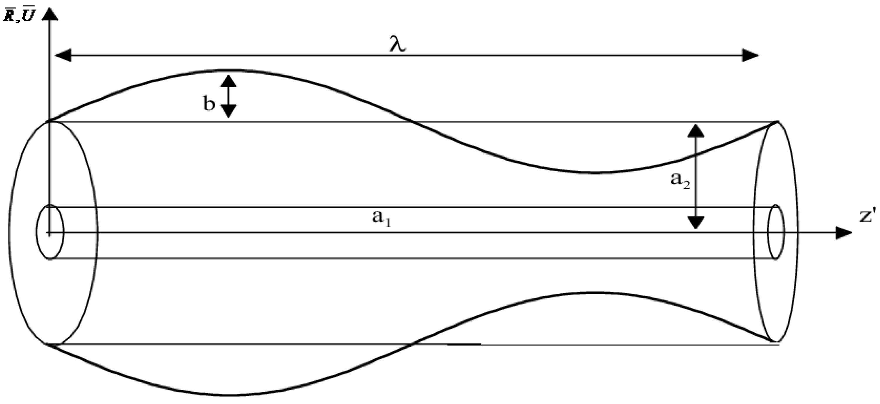
2. Mathematical Formulation
3. Solution by Adomian Decomposition Method
3.1. Case 1 (When μ = 1)
3.1.1. Volume Flow Rate and Pressure Rise
3.1.2. Stream Function
3.2. Case 2 (When μ = r)
3.2.1. Volume Flow Rate and Pressure Rise
3.2.2. Stream Function
3.3. Case 3 (When μ = )
3.3.1. Volume Flow Rate and Pressure Rise
3.3.2. Stream Function
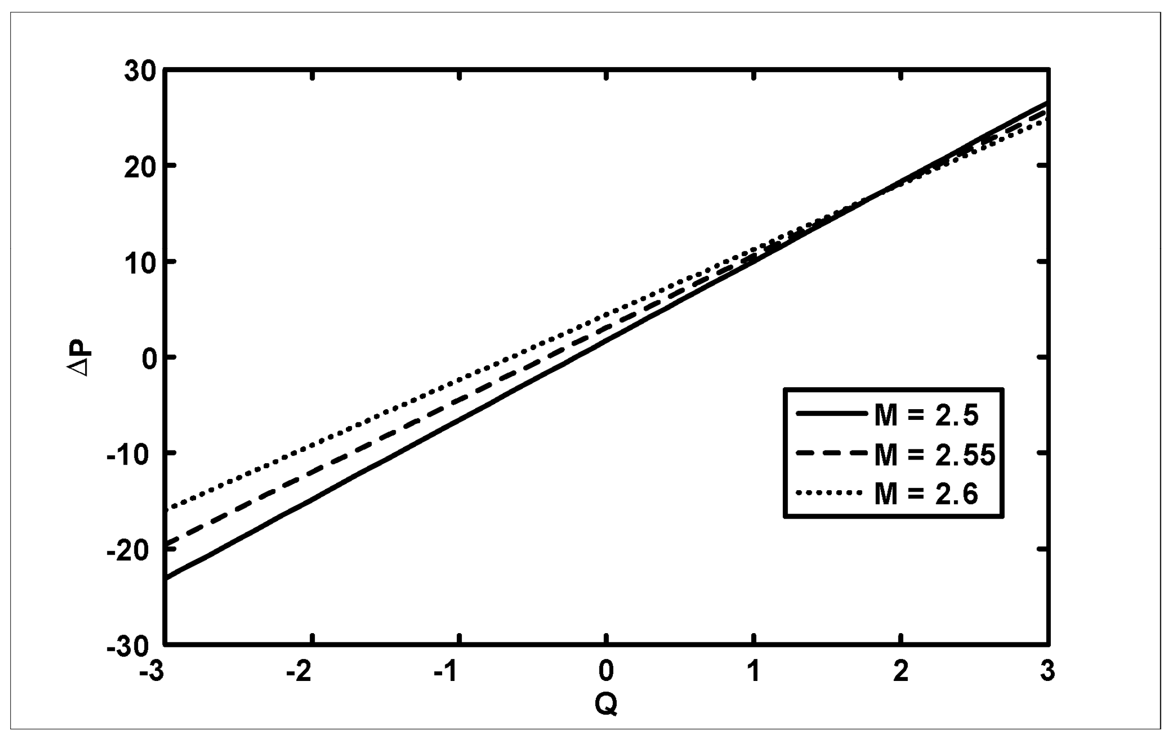
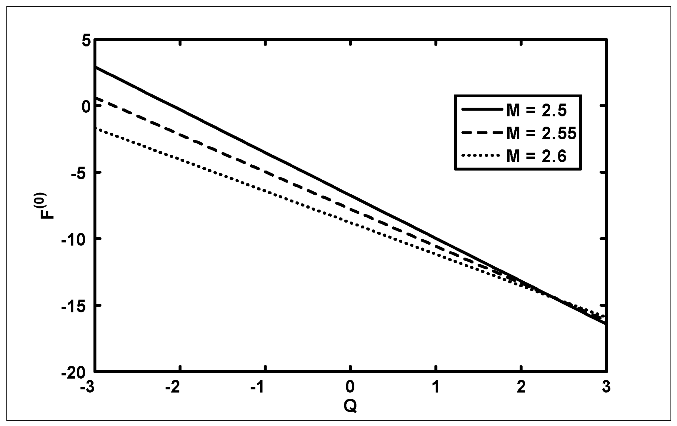
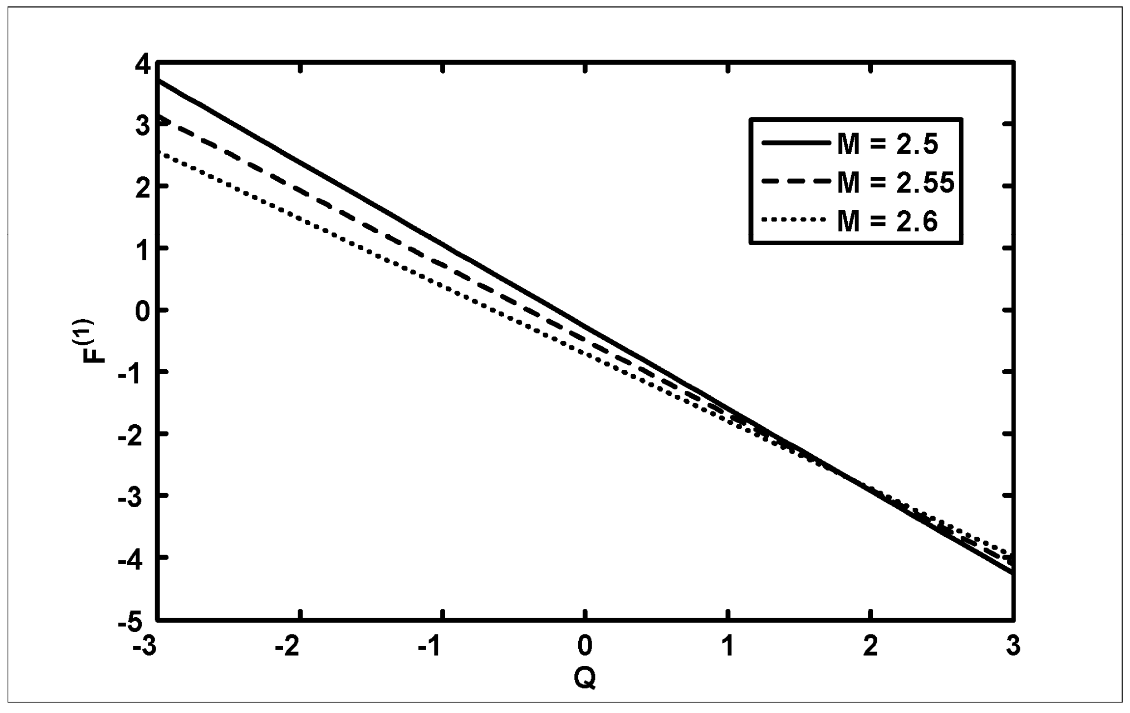
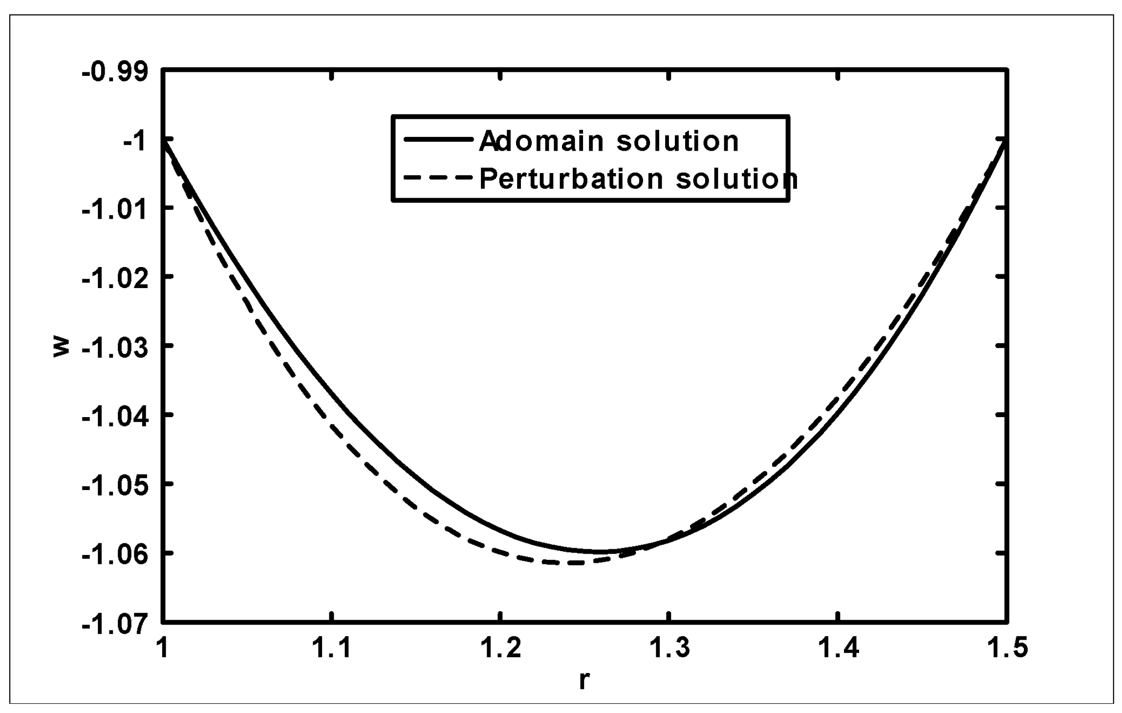
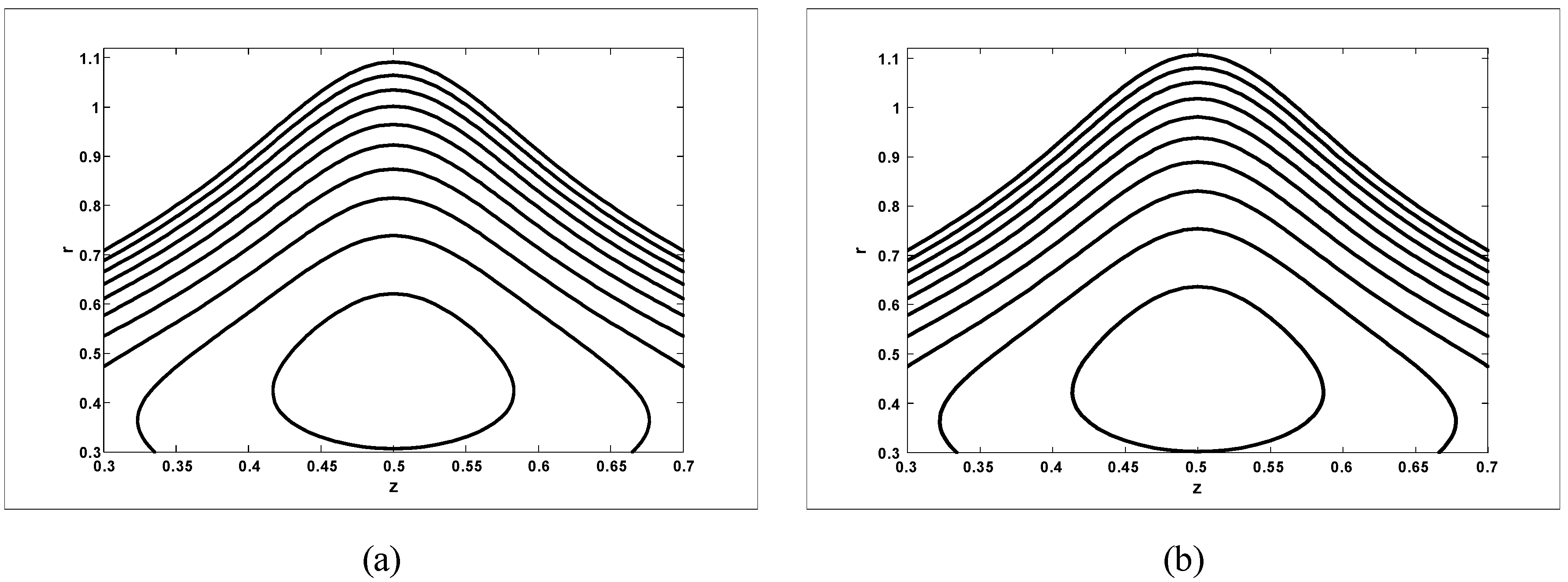
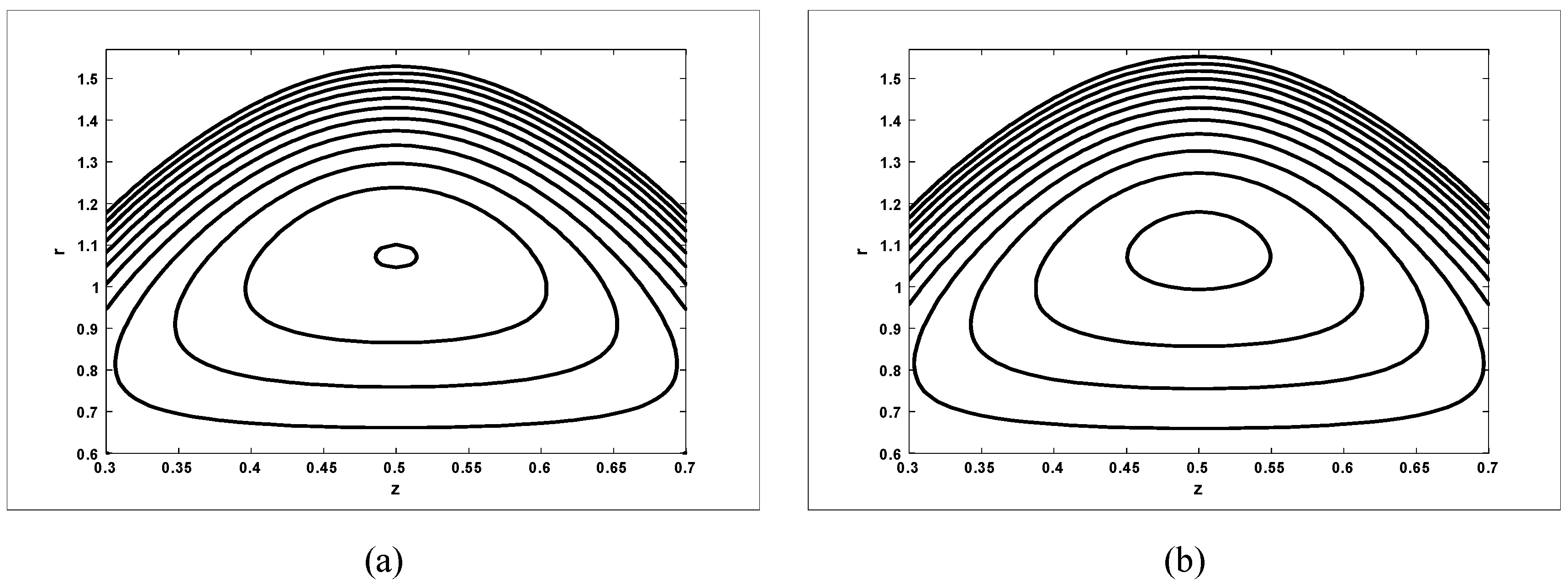
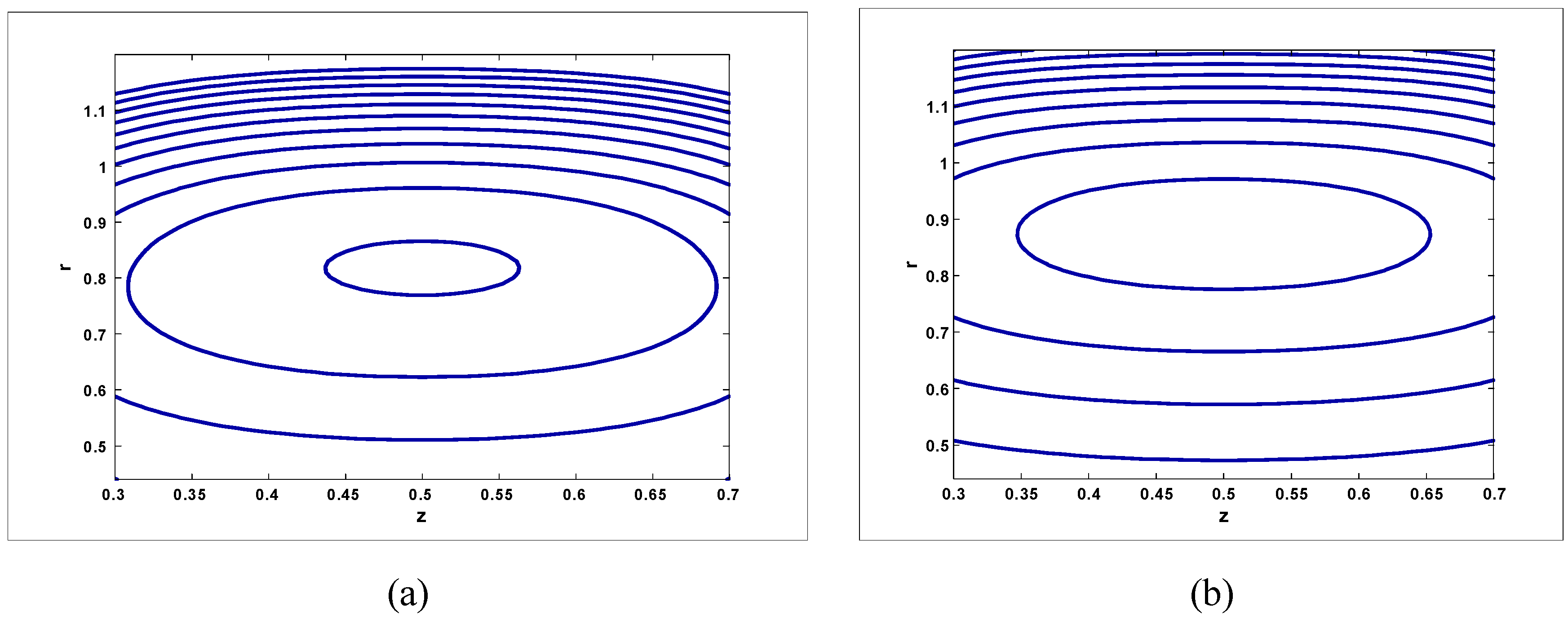
4. Results and Discussion
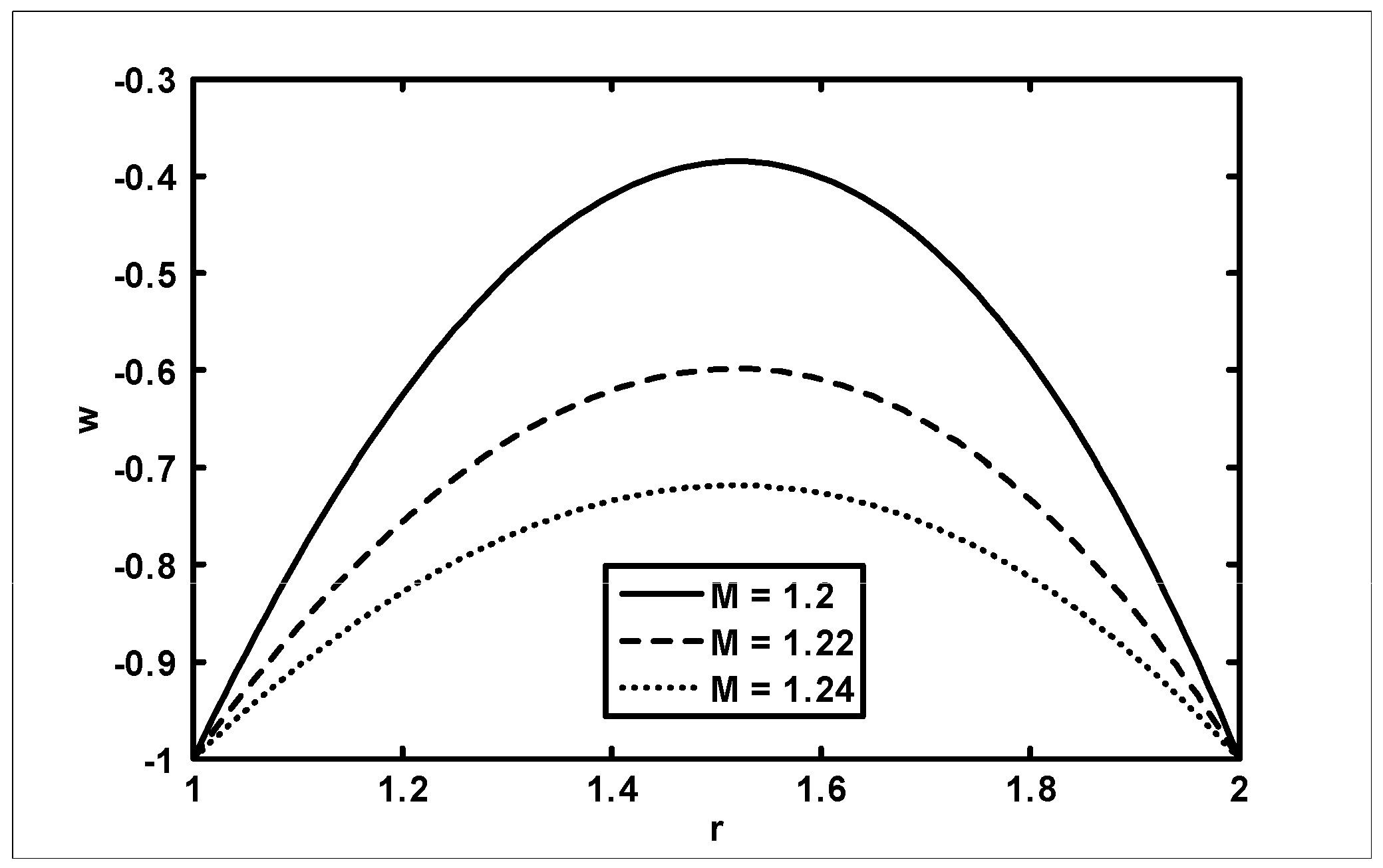
Trapping Phenomenon
5. Conclusions
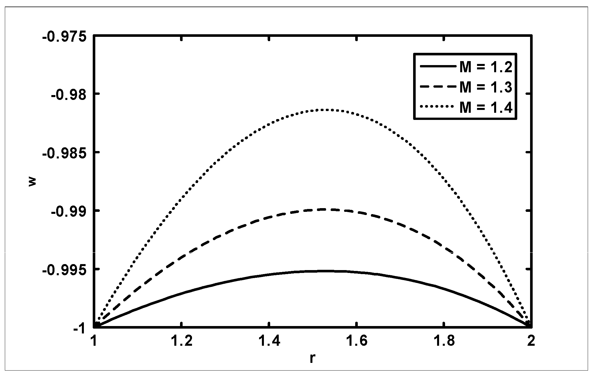
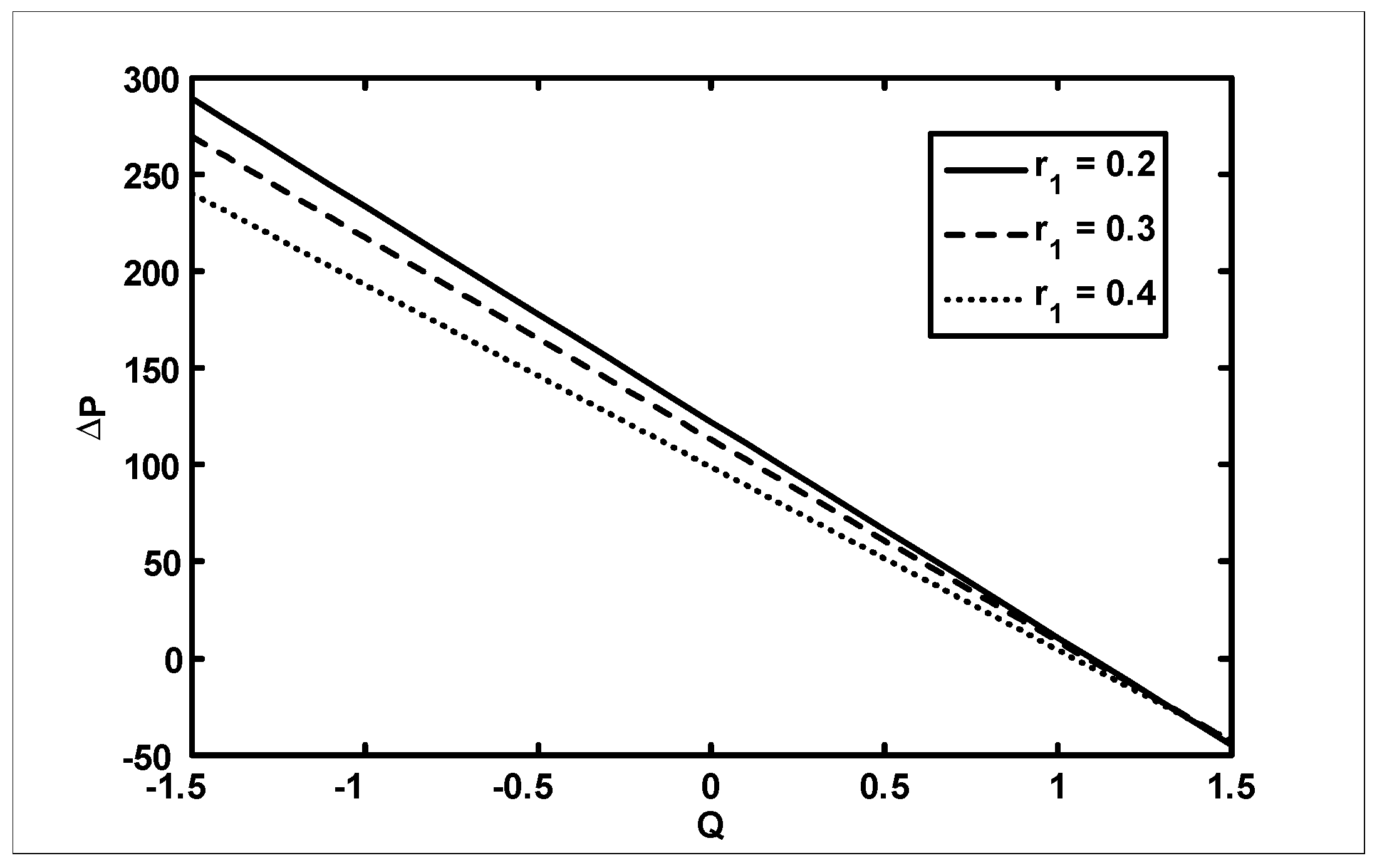
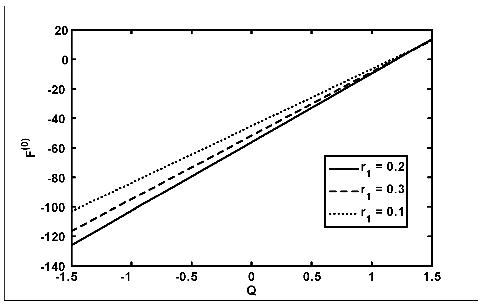
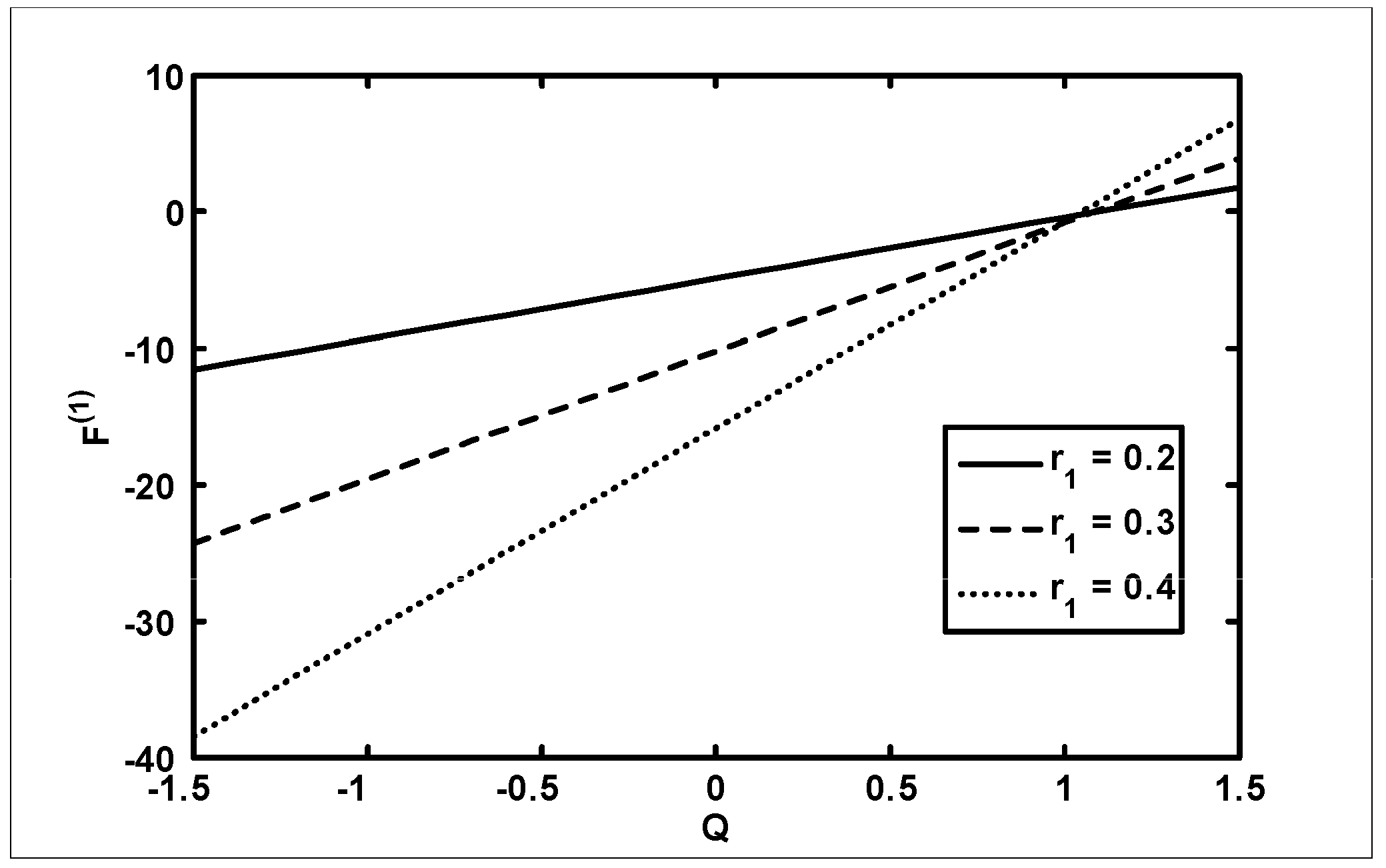
- It was found that the pressure rise increases with an increase in Hartmann number and frictional forces for the outer and inner tube decreases with an increase in when viscosity
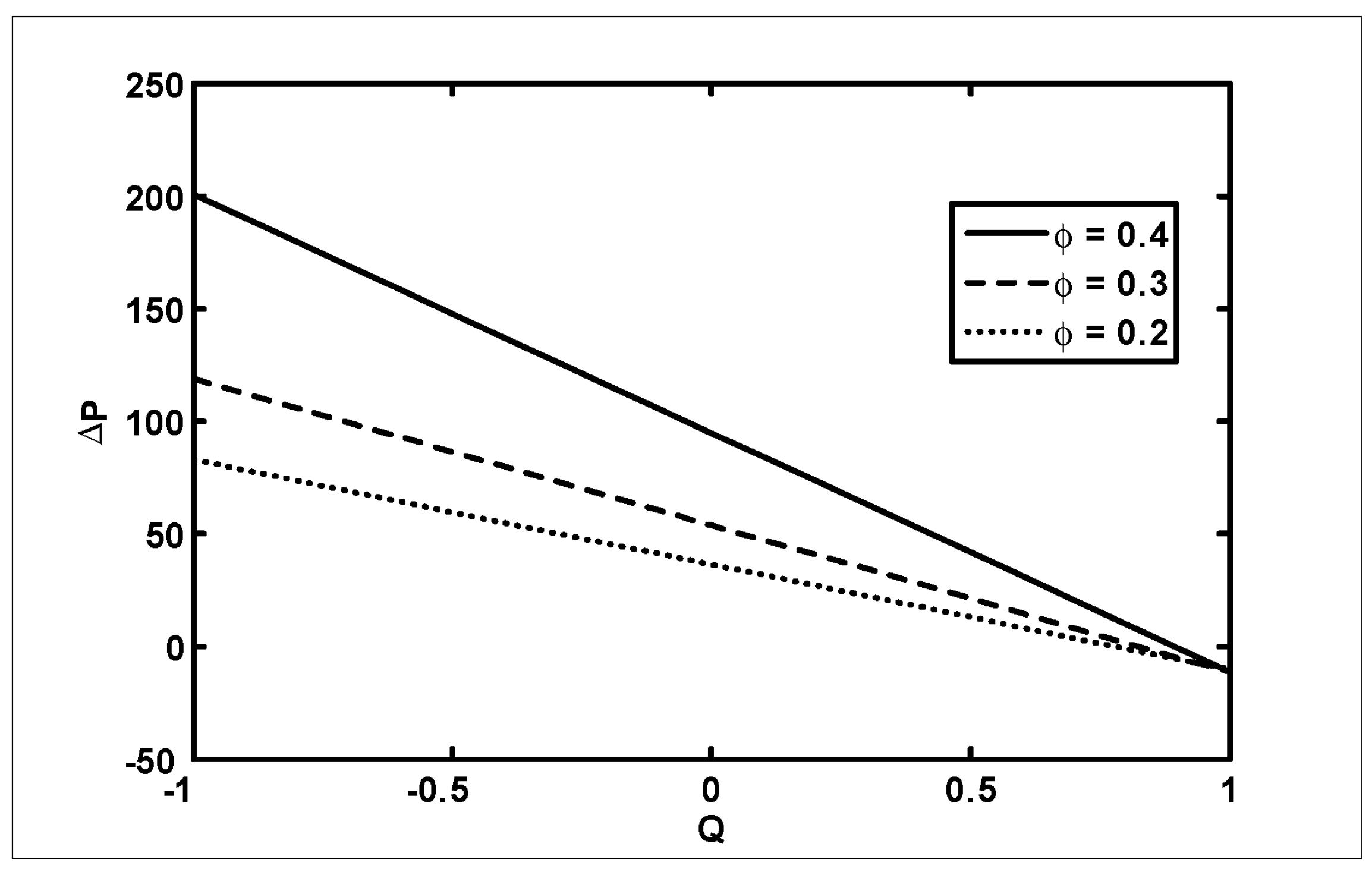
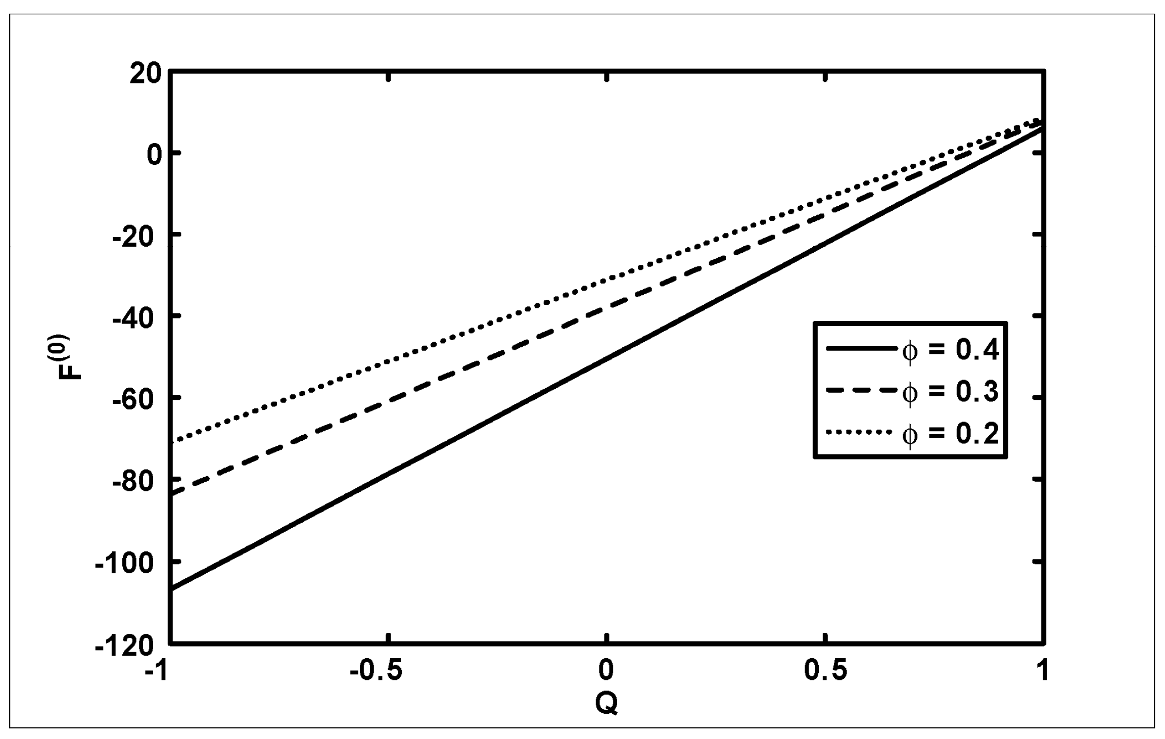
- It was also found that the pressure rise decreases with an increase in amplitude ratio in the retrograde and peristaltic pumping regions and frictional forces give opposite behavior as compared with pressure rise when viscosity
- The pressure rise decreases in the retrograde , peristaltic pumping and copuming regions with an increase in , and frictional forces decrease for small values of volume flow rate with an increase in when viscosity
- It was also noticed that the size of the trapping bolus increases with an increase in amplitude ratio when viscosity while it increases with an increase in Hartmann number and amplitude ratio when viscosity However, it decreases with an increase in Hartmann number and increases with an increase in amplitude ratio when viscosity
Author Contributions
Funding
Conflicts of Interest
Nomenclature
| and | radii of the inner and the outer tubes |
| amplitude of the wave | |
| wavelength | |
| propagation velocity | |
| Time | |
| velocity components in radial and axial directions in moving coordinates | |
| velocity components in radial and axial directions in fixed coordinates | |
| density | |
| electrically conductivity of the fluid | |
| variable viscosity | |
| amplitude ratio | |
| Reynolds number | |
| dimensionless wave number | |
| magnetic parameter | |
| Q | volume flow rate |
| and | constants used to simplify the problem |
Appendix A
| , |
| , |
| , |
| , |
| , |
| , |
References
- Abd El Naby, A.H.; El Misiery, A.E.M. Effects of an endoscope and generalized Newtonian fluid on peristaltic motion. Appl. Math. Comput. 2002, 128, 19–35. [Google Scholar] [CrossRef]
- Mekheimer, K.S. Non-linear peristaltic transport of magneto-hydrodynamic flow in an inclined planar channel. Arab. J. Sci. Eng. 2003, 28, 183–202. [Google Scholar]
- Elshahed, M.; Haroun, M.H. Peristaltic transport of Johnson-Segalman fluid under effect of a magnetic field. Math. Probl. Eng. 2005, 6, 663–677. [Google Scholar] [CrossRef]
- Ellahi, R.; Bhatti, M.; Pop, I. Effects of hall and ion slip on MHD peristaltic flow of Jeffrey fluid in a non-uniform rectangular duct. Int. J. Numer. Methods Heat Fluid Flow 2016, 26, 1802–1820. [Google Scholar] [CrossRef]
- Haroun, M.H. Effect of Deborah number and phase difference on peristaltic transport in an asymmetric channel. Commun. Non-Linear Sci. Numer. Simul. 2007, 12, 1464–1480. [Google Scholar] [CrossRef]
- Mekheimer, K.S.; AbdElmaboud, Y. Influence of heat transfer and magnetic field on peristaltic transport of a Newtonian fluid in a vertical annulus. Application of an endoscope. Phys. Lett. A 2008, 372, 1657–1665. [Google Scholar] [CrossRef]
- Ellahi, R.; Zeeshan, A.; Hussain, F.; Asadollahi, A. Peristaltic blood flow of couple stress fluid suspended with nanoparticles under the influence of chemical reaction and activation energy. Symmetry 2019, 11, 276. [Google Scholar] [CrossRef]
- Nadeem, S.; Akram, S. Peristaltic transport of a hyperbolic tangent fluid model in an asymmetric channel. Z. Nat. A 2009, 64, 559–567. [Google Scholar] [CrossRef]
- Ellahi, R.; RiazANadeem, S. A theoretical study of Prandtlnanofluid in a rectangular duct through peristaltic transport. Appl. Nanosci. 2014, 4, 753–760. [Google Scholar] [CrossRef]
- Siddiqui, A.M.; Farooq, A.A.; Rana, M.A. Study of MHD effects on the cilia-induced flow of a Newtonian fluid through a cylindrical tube. Magnetohydrodynamics 2014, 50, 249–261. [Google Scholar]
- Radhakrishnamacharya, G.; Murthy, V.R. Heat transfer to peristaltic transport in a non-uniform channel. Def. Sci. J. 1993, 43, 275–280. [Google Scholar] [CrossRef]
- Radhakrishnamacharya, G.; Srinivasulu, C. Influence of wall properties on peristaltic transport with heat transfer. C. R. Mec. 2007, 335, 369–373. [Google Scholar] [CrossRef]
- Prakash, J.; Tripathi, D.; Tiwari, A.K.; Sait, S.M.; Ellahi, R. Peristaltic Pumping of Nanofluids through a Tapered Channel in a Porous Environment: Applications in Blood Flow. Symmetry 2019, 11, 868. [Google Scholar] [CrossRef]
- Shapiro, A.H.; Jaffrin, M.Y.; Weinberg, S.L. Peristaltic pumping with long wave length at low Reynolds number. J. Fluid Mech. 1969, 37, 799–825. [Google Scholar] [CrossRef]
- Jaffrin, M.Y.; Shaprio, A.H. Peristaltic pumping. Annu. Rev. Fluid Mech. 1971, 3, 13–36. [Google Scholar] [CrossRef]
- Eberhart, R.C.; Shitzer, A. Heat Transfer in Medicine and Biology, 1st ed.; Springer: Berlin/Heidelberg, Germany, 1985. [Google Scholar]
- Pozrikidis, C. A study of peristaltic flow. J. Fluid Mech. 1987, 180, 515–527. [Google Scholar] [CrossRef]
- Eytan, O.; Elad, D. Analysis of intra-uterine fluid motion induced by uterine contractions. Bull. Math. Biol. 1999, 61, 221–238. [Google Scholar] [CrossRef] [PubMed]
- Riaz, A.; Al-Olayan, H.A.; Zeeshan, A.; Razaq, A.; Bhatti, M.M. Mass Transport with Asymmetric Peristaltic Propulsion Coated with Synovial Fluid. Coatings 2018, 8, 407. [Google Scholar] [CrossRef]
- Abd El Naby, A.; El Misery, A.E.M.; El Shamy, I.I. Effects of an endoscope and fluid with variable viscosity on peristaltic motion. Appl. Math. Comput. 2004, 158, 497–511. [Google Scholar] [CrossRef]
- Mekheimer, K.S.; AbdElmaboud, Y. Simultaneous effects of variable viscosity and thermal conductivity on peristaltic flow in a vertical asymmetric channel. Can. J. Phys. 2014, 92, 1541–1555. [Google Scholar] [CrossRef]
- Husseny, S.Z.A.; AbdElmaboud, Y.; Mekheimer, K.S. The flow separation of peristaltic transport for Maxwell fluid between two coaxial tubes. Abstr. Appl. Anal. 2014, 2014, 269151. [Google Scholar] [CrossRef]
- Adomian, G. Non-Linear Stochastic Operator Equations; Academic Press: Orlando, FL, USA, 1986. [Google Scholar]
- Adomian, G. Solving Frontier Problems of Physics: The Decomposition Method; Kluwer Academic Publishers: Boston, MA, USA, 1994. [Google Scholar]
- Eldabe, N.T.; Elghazy, E.M.; Ebaid, A. Closed form solution to a second order boundary value problem and its application in fluid mechanics. Phys. Lett. A 2007, 363, 257–259. [Google Scholar] [CrossRef]
- Wazwaz, A.M. Exact solutions to nonlinear diffusion Equations obtained by the decomposition method. Appl. Math. Comput. 2001, 123, 109–122. [Google Scholar] [CrossRef]
- Wazwaz, A.M. A new method for solving singular initial value problems in the second order ordinary differential Equations. Appl. Math. Comput. 2002, 128, 47–57. [Google Scholar] [CrossRef]
- Wazwaz, A.M. Partial Differential Equations, Method and Applications; Balkema Publishers: Avereest, The Netherlands, 2002. [Google Scholar]
- Wazwaz, A.M. Adomian decomposition method for a reliable treatment of the Emden-Fowler equationuation. Appl. Math. Comput. 2005, 161, 543–560. [Google Scholar]
- AbdElmaboud, Y.; Mekheimer, K.S.; Abdelsalam, S.I. Study of nonlinear variable viscosity in finite-length tube with peristalsis. Appl. Bionics Biomech. 2014, 11, 197–206. [Google Scholar] [CrossRef]


© 2019 by the authors. Licensee MDPI, Basel, Switzerland. This article is an open access article distributed under the terms and conditions of the Creative Commons Attribution (CC BY) license (http://creativecommons.org/licenses/by/4.0/).
Share and Cite
Akram, S.; H. Aly, E.; Afzal, F.; Nadeem, S. Effect of the Variable Viscosity on the Peristaltic Flow of Newtonian Fluid Coated with Magnetic Field: Application of Adomian Decomposition Method for Endoscope. Coatings 2019, 9, 524. https://doi.org/10.3390/coatings9080524
Akram S, H. Aly E, Afzal F, Nadeem S. Effect of the Variable Viscosity on the Peristaltic Flow of Newtonian Fluid Coated with Magnetic Field: Application of Adomian Decomposition Method for Endoscope. Coatings. 2019; 9(8):524. https://doi.org/10.3390/coatings9080524
Chicago/Turabian StyleAkram, Safia, Emad H. Aly, Farkhanda Afzal, and Sohail Nadeem. 2019. "Effect of the Variable Viscosity on the Peristaltic Flow of Newtonian Fluid Coated with Magnetic Field: Application of Adomian Decomposition Method for Endoscope" Coatings 9, no. 8: 524. https://doi.org/10.3390/coatings9080524