Urban Mobility Demand Profiles: Time Series for Cars and Bike-Sharing Use as a Resource for Transport and Energy Modeling


1
Fondazione Eni Enrico Mattei, corso Magenta 63, 20123 Milano, Italy
2
Politecnico di Torino, corso Duca degli Abruzzi 24, 10129 Torino, Italy
3
Politecnico di Milano, Via Lambruschini 4c, 20156 Milano, Italy
*
Author to whom correspondence should be addressed.
Data 2019, 4(3), 108; https://doi.org/10.3390/data4030108
Submission received: 20 June 2019
/
Revised: 19 July 2019
/
Accepted: 25 July 2019
/
Published: 26 July 2019
Abstract
:The transport sector is currently facing a significant transition, with strong drivers including decarbonization and digitalization trends, especially in urban passenger transport. The availability of monitoring data is at the basis of the development of optimization models supporting an enhanced urban mobility, with multiple benefits including lower pollutants and CO2 emissions, lower energy consumption, better transport management and land space use. This paper presents two datasets that represent time series with a high temporal resolution (five-minute time step) both for vehicles and bike sharing use in the city of Turin, located in Northern Italy. These high-resolution profiles have been obtained by the collection and elaboration of available online resources providing live information on traffic monitoring and bike sharing docking stations. The data are provided for the entire year 2018, and they represent an interesting basis for the evaluation of seasonal and daily variability patterns in urban mobility. These data may be used for different applications, ranging from the chronological distribution of mobility demand, to the estimation of passenger transport flows for the development of transport models in urban contexts. Moreover, traffic profiles are at the basis for the modeling of electric vehicles charging strategies and their interaction with the power grid.
1. Introduction
The transport sector has gained importance in view of ambitious goals aiming at decarbonizing all the sectors of our economy within 2050. The transport sector, in 2016, accounted for 2748 Mtoe, almost 28% of the total final consumption (TFC) at global level. Oil products covered a share of 92% of it while the remaining share was satisfied by other vectors like natural gas, biofuels and electricity. Considering the mode of transport, 75% of demand was related to road vehicles, followed by aviation and navigation [1]. On emissions side, in 2015, surface passenger mobility and freight transport accounted for 78% of global transport emissions according to ITF database [2]. According to Gota et al. [3], transport sector mitigation potential can be fully released throughout measures that include reduction of demand, shifting to more efficient modes of transport and improved performance of vehicles and fuels.
The global picture highlights the need for targeted actions towards carbon-free transport systems, specifically for the road sector. The decarbonization of surface passenger mobility is mainly related to the electrification of demand and the improvement of the system efficiency. Higher efficiency can be attained by fostering the integration of modes of transport in order to curb the overall transport demand as well as enhancing technology performances. In this regard, mobility as a service (MaaS) and digitalization play a crucial role. Integrated schemes of ticketing, fares and service information as well as service and physical coordination are some of the next challenges passenger transport sector will need to face according to ITF report on public services and cycling integration [4]. In addition to that, Lazarus et al. [5] report that shared mobility has already proven some beneficial effects on urban environment such as the reduction of car congestion, vehicle ownership rates, transport demand and emissions. However, other studies [6] point out that transportation network companies, such as Uber and Lyft, are the biggest contributors to the increase of congestion in cities such as San Francisco. The availability of real data is crucial to understand these complex phenomena and to support an optimized regulation and development of digital technologies in transport [7], including shared mobility.
In order to assess the impact of such a paradigm shift, modeling tools are necessary. In transport modeling, the objective is mainly related to congestion management, transport planning and emissions reduction. The geographical scale of applications can vary according to the aim of the study. Urban modeling is extremely dependent on geographical context as reported by several case studies implemented in MATSim framework [8]. Usually, the inputs of these models are based on mobility surveys that reproduce a synthetic population representative of a particular area. The data collected include the number of trips, activity purposes, duration, modes, departing and arrival time and the origins and destinations of trips. The mobility issue is extremely dependent on people’s choices and behaviours as reported in the work of Martinez et al. [9], so agent-based modeling (ABM) represents a good framework that can simulate complex dynamics and what-if scenarios, usually in the short and medium run. Modeling such dynamics requires high temporal detail that is usually based on a hourly timestamp. Also system dynamics can be used to model part of the transport sector, as in the case of a car stock evolution simulation model implemented into the TIMES (The Integrated MARKAL-EFOM System) framework [10]. In this case, the temporal resolution is lower and extended to one year since the focus is on car adoption.
According to IEA, the electrification of sectors can lead to an increase of efficiency of consumption and a higher renewable penetration as reported in WEO 2018 [11]. Electrification only is not sufficient to achieve the climate targets but it can contribute to lowering the fossil fuel consumption and emissions. The impact of transport sector electrification depends on the integration level with power sector so it is necessary to develop a sector-coupling modeling approach. In this regard, the literature is rich of studies that range from integrated assessment models (IAM), at global scale, such as MESSAGE and GCAM to energy models with higher technical resolution such as TIMES for the Danish case [12,13]. Regarding IAMs, modeling details of behavioural aspect of vehicle adoption rates, modal choice, urban congestion and urban vs rural considerations are completely missing [14]. Instead, studies with higher detail of both transport and power sectors are usually limited to lower geographical coverage.
Hourly profiles are needed when intermittent renewable energies, electric vehicles and, in general, electricity storage come to play. Moreover, mobility dynamics need to be considered on hourly basis in order to properly distribute the vehicles’ consumption on the aggregate electric load. Andersen et al. [15] developed an hourly-detailed scenario tailored on the Danish case, but the electric vehicles’ charging profile has been assumed constant during the day. Besides, the day-time load represents one third of the total daily charging demand. If the objective is to evaluate the impact of electric vehicles on the electric load peaks, the approach selected is insufficient due to lack of passenger behaviours dynamics that affect charging strategies.
Transport demand profiles are very context-specific so the necessity of collecting big amount of data arises if the temporal resolution wants to be ensured. The collection procedures are several and they range from sensor readings to social sensing from street-level imagery as included in the study of Zhang et al. [16] in which taxis’ trips are used as proxy to develop a forecast model of the city traffic. Jelica et al. [17] used the traffic data referring to light duty vehicles (cars and light-weight trucks) and heavy duty vehicles (trucks and buses) in order to assess the theoretical impact of electric road systems (ERS) on the electrical network assuming 100% electrification of traffic. The ERS application well describes the need for hourly traffic profiles that are translated into a hourly electricity demand.
In [18], Sekula et al. develop an artificial neural network (ANN) model in order to estimate historical traffic demand in Maryland. The study is based on two main data sources: a dataset referring to automated traffic recording (ATR) sampled on hourly-basis from 45 stations (90 one-directional carriageways). Besides, vehicle probe volumes and vehicles probe speeds [19] are used to enrich the range of inputs of ANN model. In this case, the sampling occurs every 30 min.
Data acquisition campaigns can have limited duration, such as in case of the study on integrated urban transportation master plan for Istanbul metropolitan area [20]. The data collection started on 14 June and finished on 24 May, sampling traffic values in specific time windows from 7 a.m to 10 a.m, from 12 a.m to 2 p.m and finally from 5 p.m to 8 p.m. The campaign relied on 351 counting station, sampling with a frequency of one hour.
Motor vehicles do not solely compose the modes of transport portfolio available in cities. Soft modes like walking and biking are good alternatives as well as, specifically, mobility services such as bike sharing and e-scooters. Since collection of data for bike sharing is already performed and mainly automatized, greater quantity of profile datasets are available. Oppermann et al. [21] developed a platform that keeps track of several bike sharing profiles of different cities. The goal is not limited to the analysis of cycling behaviours but also to figure out high-level city dynamics that in general can affect mobility patterns. Some detailed analyses have been performed based on single cities [22] or on the comparison of multiple cities [23], or with more specific focuses such as the effect of weather conditions ([21,24]) or the comparison with the use of e-scooters [25].
Concerning bicycle volumes, Jestico et al. [26] use datasets provided by institutions (regional bike count program) and private sector as well. In the fist case, 18 locations are equipped by meters providing, by the way, very limited information due to a selected time window within the day and recordings relative to a few days in four different months. In total, the sampling occurs in 34 different days aiming at depicting the seasonal variability. In the case of crowd sourced data, cycling dataset is collected by means of an app. Spatial and temporal resolutions are extremely high, in particular the sampling time reaches 1 min. On the contrary, the size of the sample is limited to whom subscribes to the application.
Safe-D [27] published a report in which the number of vehicles and bikes can be correlated to the decrease of vehicle speed. In order to perform such analysis, data from different sources have been merged. First of all, bicycle volume has been obtained thanks to the data provided by the San Diego Regional Bike and Pedestrian Counter Network [28]. The sampling procedures is based on data acquisition from 49 sites, every 15 min, 24 h per day. Moreover, the model developed by Safe-D, relies on pneumatic road tube data composed by both the number of bikes and speed. The sampling duration ranges between one and two weeks and data are aggregated in 15-min time slices. Included in the report, purchasing of volume/speed data is mentioned. Vendors collect crowdsourced data with remarkable spatial coverage (data related to road-segment), identifying also the direction bike flows.
The main purpose of this paper is to provide to the readers an open dataset with a very high time resolution (five-minutes over an entire year), that can be used as a support for transport modeling. The dataset includes information about bikes utilization (through bike-sharing data) and vehicles traffic flows for the same city. Together with an accurate description of the available data, a brief analysis of the load profiles is presented, to provide the readers with a preliminary summary of the main features of these datasets.
2. Materials and Methods
This paper presents two datasets that can be used to define a chronological distribution of the mobility demand in an urban context. The first dataset is related to the vehicle flows of some main roads measured by different sensors across the city, while the second is related to the utilization of the station-based bike sharing system of the city.
The data are related to the city of Turin, located in the North–West of Italy, with almost 900,000 inhabitants (and 1.4 million considering the neighbouring municipalities). Turin is the regional capital of Piedmont, and it includes a significant number of people from neighbouring municipalities that travel daily to Turin for work or study purposes.
Although a share of commuters travel by train, available data for Italy [29] shows that currently 71.3% of the mobility for working purposes is performed by car. As a result, the commuters mobility from neighbouring towns is a significant share of the total traffic in Turin. This phenomenon is common to other cities (e.g., Milan) that have a concentration of working activities, but it is less pronounced in smaller cities, which may have weaker traffic variation over the day.
2.1. Vehicles Profiles
The municipality of Turin has a traffic monitoring system that includes the measurement of traffic flows and speeds in several roads across the city. A part of the sensors data is available as open data [30], and it is at the basis of the data analysis presented in this paper. Since the sensors are not covering the entire road network, they are not suitable to derive absolute numbers of vehicle flows. Indeed, they are a good measurement of the daily (and seasonal) variation of the vehicles flows and speeds, from which an aggregated measurement will be presented.
The data are representing the flow of all the vehicles, including cars, commercial vehicles, buses, etc. Although there is no detailed information on the type of vehicles, the large majority of traffic in city is related to private cars, especially considering that the sensors are not measuring any flow related to highway traffic. Some data for the Limited Traffic Zone (LTZ) in the city center [31] shows that around 90,000/120,000 vehicles access the LTZ of Turin every day, of which only 2500 are freight transport vehicles. For this reason, we believe that the measured data on vehicle flows can represent the patterns of private cars usage.
2.1.1. Raw Data
The raw data refers to around 160 traffic sensors installed on almost 50 different streets of the city, evenly distributed across the metropolitan area. This dataset is limited to the data that is available to the public as open data, which includes information on the vehicles flow and average speed, measured every five minutes and published in real time [30]. The data is provided under the Italian Open Data License v2.0 [32].
There is no historical record of these data, and therefore it has been necessary to implement a proper automated routine to collect and store this information. For the purpose of the present study, the data has been extracted for the entire year 2018.
Data acquisition is performed by a Perl script hosted on a server and running every five minutes, in accordance with the refresh time provided by the website. At each iteration, the script retrieves the most recent XML file from the website [30].
The XML tree is composed by a root element called traffic_data, which stores information on the data source and the starting and ending time of the measurements, which are common to all the data reported in the file. Each node of the file is representing a specific measurement location, for which information is given on the road name, the position, the direction etc. For each of these nodes an additional element is available with the measured flow and speed for the vehicles.
The information available in the XML file is parsed by the script to produce tabular data in csv format, which is appended to a text file with the previous iterations. The first execution of the day generates a new text file, so the data is stored in a file for each day, to limit the file size and minimize the potential impact of failures and errors. The choice of storing tabular data instead of XML files is related to the very simple and repetitive structure of the data, which would not benefit from the additional flexibility provided by the XML format.
The raw dataset, constituted by roughly 10 M records, includes information on the average traffic flow and speed of the vehicles, with no information of the kind of vehicles nor on the characteristics of the streets where the sensors are installed. Since the aim of this work is to provide a chronological distribution that can be applied to other similar urban contexts, the data have been aggregated to define a global traffic profile of the city.
2.1.2. Data Processing
Unfortunately, the quality of the data is affected by a significant number of records with low accuracy. For each measured value of vehicles’ speed and flow, a corresponding measure of accuracy is provided, ranging from 0 to 100. this accuracy is related to the quality of the measuring instrument, and it provides the percentage of reliable data that has been measured on any given time step. On the entire number of records for 2018, only 82.6% has a quality larger than 90, which is the threshold considered in this work to filter out the non reliable data.
In particular, there is a systematic low accuracy in the first record of each day, related to a technical issue of sensor reset. For this reason, the statistics related to those times frames appear to be quite biased. However, they have been included into the dataset to maintain the largest possible information.
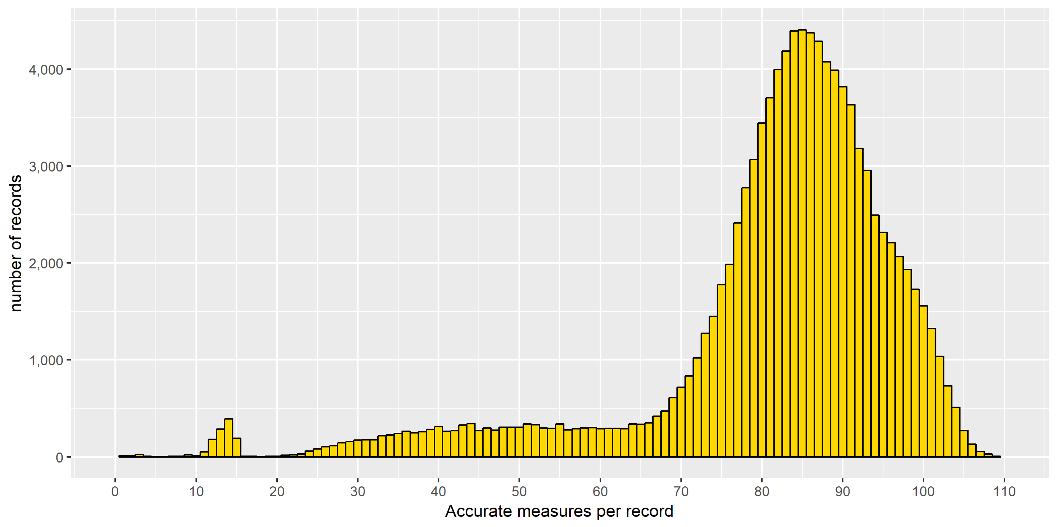
For each record, a specific column reports the number of sensors on which the aggregations have been performed (i.e., with an accuracy value larger than 90). This may help the readers in filtering out data with an undesired reliability. Our suggestion is to filter out the data records based on less than 60 sensors, which appears to be a good balance between a minimum number of sensors and a good number of records (see Figure 1).
2.1.3. Output Data
The output dataset that is provided alongside this paper (filename: “cars.csv”), reports the following information for each available five minute time interval:
- Starting time
- n: number of accurate sensors on which the statistics are based
- mean, standard deviation and median value for the vehicles flow
- mean, standard deviation and median value for the vehicles speed
These data are provided for the entire year 2018, with some missing data points related to data that were not available from the measurements. A systematic missing data point occurs each day at 23.55, due to a system reset, resulting in no update of the data on the database.
The output file is composed by a total of 104,117 records, each of them is referring to a 5 min interval in the year (i.e., with less than 1% missing data). Each record is based on a number of measurements ranging from 1 to 198, depending on the availability of the information published in the XML file described above, but with a median value of 85 (see Figure 1). The values related to the average vehicle flow range from 12 to 1675 vehicles/hour, with a median of 470. The corresponding average vehicle speed lays in the interval 18–58 km/h, with a median value of 29.5.
2.2. Bike Sharing Profiles
The first bike sharing system of Turin, named ToBike, became operational in the summer of 2010. In these 9 years the system has reached around 9 million trips, with an estimated total distance of 38 million km [33]. There are currently 128 stations in operation, with 26 more in planning that will be available in the next few months. The available bikes, roughly 1100, are used by almost 30,000 annual subscribers and by occasional users.
2.2.1. Raw Data
The data related to bike sharing operation in Turin has been retrieved from the live status of the docking stations in Turin each 5 min, to build up a significant historical trend (October 2016–May 2019). However, since these years are characterized by an evolution of the available docking stations and the users subscriptions, for the purpose of this work only the data related to 2018 are provided. This choice has the double advantage of providing a dataset that is consistent with the one available for traffic flows, and at the same time avoid the effect of the variation of annual subscriptions of the bike sharing system.
The live data is available at [33] as html code, which is parsed to extract the information about each station. The available data is limited to the status of each station (i.e., number of available bikes, number of free places). Additional information related to the trip is not available, nor it is possible to know the total number of bikes or the number of users of the system.
Also in this case, the data is gathered through a Perl script running every five minutes and hosted on the same server cited above. In this case, the script is not directly pointing to an XML file but it reads the bike sharing system public web page [33] and parses it to extract the required information about the status of each station.
The script parses the HTML code of the web page to find all the table rows that are related to the stations, which are defined by a proper CSS class. For each row, the script extracts the cells that are related to the name of the station, its ID, the number of available bikes, available places and bikes out of order, if any. Each row is then stored as a record, and the entire web page is codified as a text file in csv format. For each iteration of the script, the resulting information is saved by appending it to a single text file for each day. The first execution of the day generates a new text file, so the knowledge is stored in a file for each day.
As already mentioned, the bike sharing in Turin has seen a continuous evolution, both in terms of stations and bikes increases, and in particular in the last two years the appearance of free-floating alternative may have had an impact on the flow patterns. Conversely, the authors believe that the use of free-floating bikes would result in very similar utilization profiles, and thus the mobility patterns at urban level remain comparable.
2.2.2. Data Processing
As described above, the available data is limited to the real-time conditions of the stations throughout the city (i.e., available bikes and free places). Thus, there is a need of data processing to estimate the flows from the available states.
Data has been collected through an automated routine every 5 min. At a given timestamp, for each station, we calculate the difference from the previous timestamp in terms of number of bikes available, obtaining the number of pick-ups (if positive) or drop-offs (if negative). The number of pick-ups will be used in this paper to analyze and discuss the number of trips, thus considering the start of each trip. A very similar profile can be obtained by considering the drop-offs, with a slight shift that is related to the trip duration. A previous study based on more detailed data ([34]), which has been limited to the month of May 2013, has calculated an average of 16.5 min of trip duration and a mode of seven minutes. It has to be highlighted that in the pricing conditions in Turin, the users can use the bike for free up to 30 min.
Unfortunately, this approach has a strong limitation: in any given timestamp difference, only pick-ups or drop-offs can be considered. In the case of contemporary pick-ups and drop-offs in any given station (in the same five minute time slot), the calculation would be able to consider only the difference.
While this aspect may lead to non-negligible errors when considering the total number of trips on a daily or monthly basis, we believe that the effect of this bias on the utilization profiles is very limited. This effect can be further limited by narrowing the duration between two timestamps. However, given the need of collecting a huge amount of data, a five minute time slot has been considered as an acceptable approximation to avoid too heavy data collecting and processing requirements. Moreover, since the status of the stations is updated by the system each three minutes, five minutes appears to be a good choice to avoid oversampling.
2.2.3. Output Data
The output data, which is available as a single csv file in the Supplementary Material of this paper (named “bikes.csv”), is provided as the total number of pick-ups and drop-offs for every five minute time interval along the year 2018.
The output file is made up by 104,834 records, with less than 0.3% of missing data points. The pick-ups range from 0 to 207, while the drop-off from 0 to 186. Both data series have an average of 12.3 and a median of 10.
We believe that providing the data in the most raw form, although already aggregated, could be more useful for the readers. However, since the main value of these data is to provide information on chronological distribution, a normalization is strongly recommended.
Moreover, it has to be noted that in this case, the bike sharing system is still in an evolutionary phase, whereas the previous dataset related to the vehicles traffic is representing a more stationary situation. However, over a single year this effect may be rather limited, since the majority of users has an annual membership, which is likely to start in spring.
3. Results
This section will present the main features of the two datasets considered in this study, with the aim of providing preliminary insights for the readers that are interested in using these data. The analysis presented in this section has been performed by using the language R [35] and some of the packages collected into the Tidyverse [36].
While the entire datasets were provided in the Supplementary Materials of this paper, this section will be focused on the main trends that emerge from the utilization profiles, rather than presenting in detail the entire time series.
3.1. Road Traffic
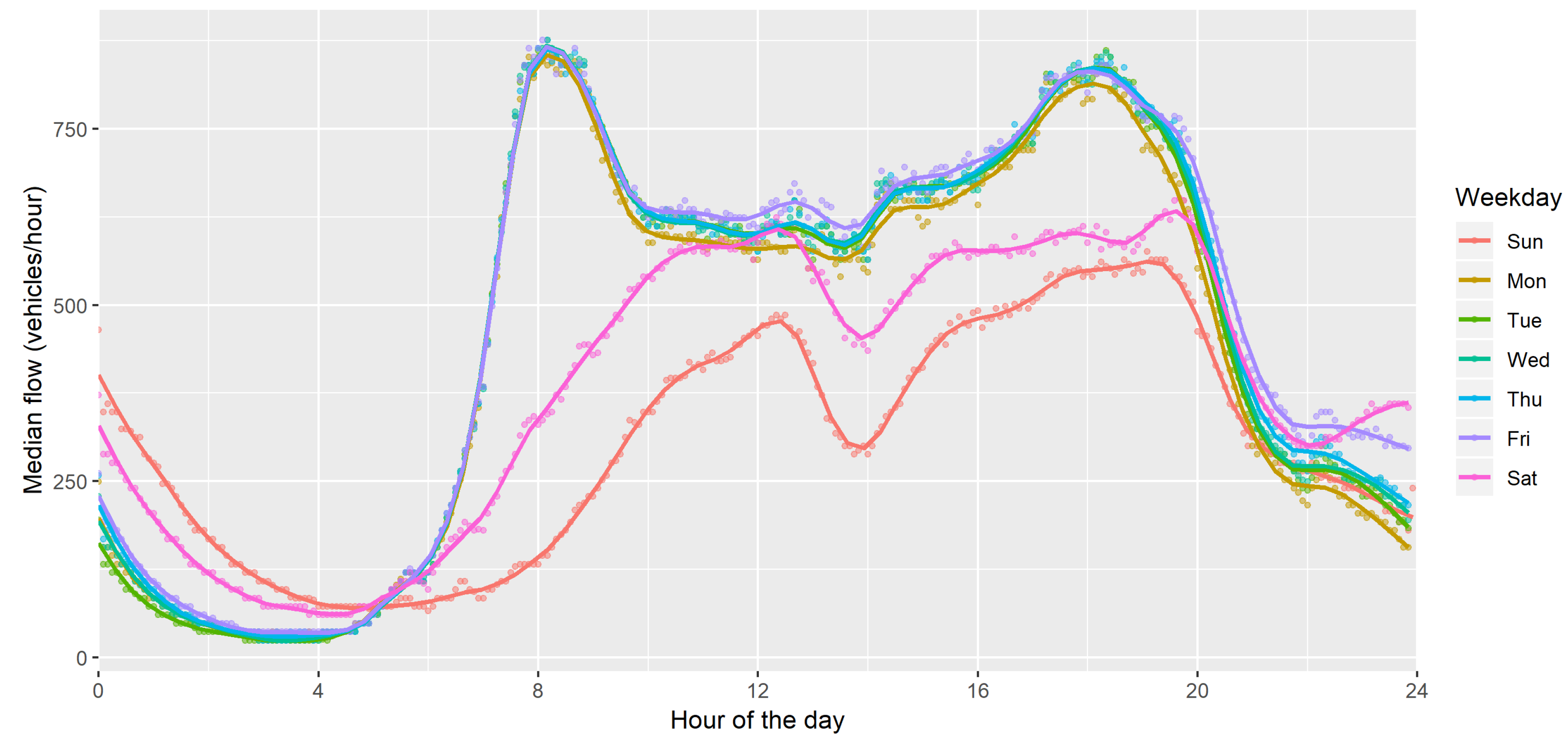
Figure 2 reports an aggregation of the vehicles measurements based on the day of the week. Each data point represents the median value of the vehicle flow, grouped by the 5 min time interval and the day of the week. This aggregation allows to analyze representative profiles by evaluating the variability related to the particular weekday, as will be better described below. The interpolation lines are drawn by locally estimated scatterplot smoothing (LOESS), which is commonly used in econometrics, and is a strongly related non-parametric regression method that combines multiple regression models in a k-nearest-neighbor-based meta-mode. The purpose of the fitting line is to provide a visual approximation of the evolution of the profile, by limiting the variability that would be caused by drawing a line through each single point.
While working days present a very similar profile, Saturday and Sunday profiles were very different, with a lower demand during the day, as well as a slight increase in the first hours of the day (which are related to higher activity on Friday and Saturday evenings). Moreover, while in working days there are two distinct peaks in the morning (around 8 AM) and in the evening (around 6 p.m), during the weekend the morning peak is translated to midday, and both peaks are less pronounced than during weekdays.
Another differentiation, although less pronounced, appears on a seasonal basis. Figure 3 reports the median vehicles profiles grouped by time interval and by month (considering working days only), with clear evidence of low usage in August and similar values for the other months (except July, which was slightly affected by holidays as well).
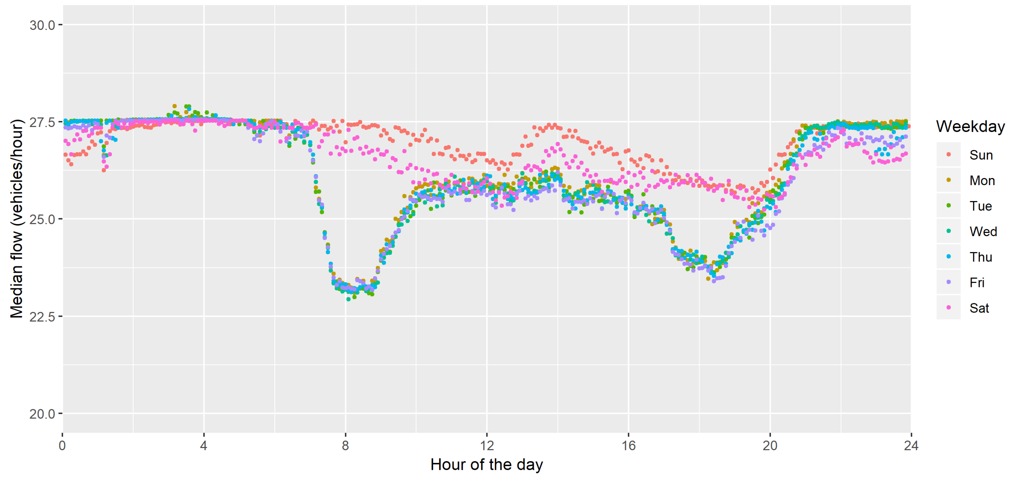
Finally, Figure 4 reports the median speed of the cars in the city, calculated with the same aggregation considered for the traffic flow in Figure 2. The vehicles’ speed appears to be strictly related with the vehicles flows seen before: the higher the flow, the lower the speed. It is worth noticing that the median speed in the city is well below 30 km/h, even during the night, although in many roads the limit is set to 50 km/h. An average speed of 27.5 km/h appears to be imposed by traffic lights and/or roundabouts at the endpoints of the road.
3.2. Bike Sharing
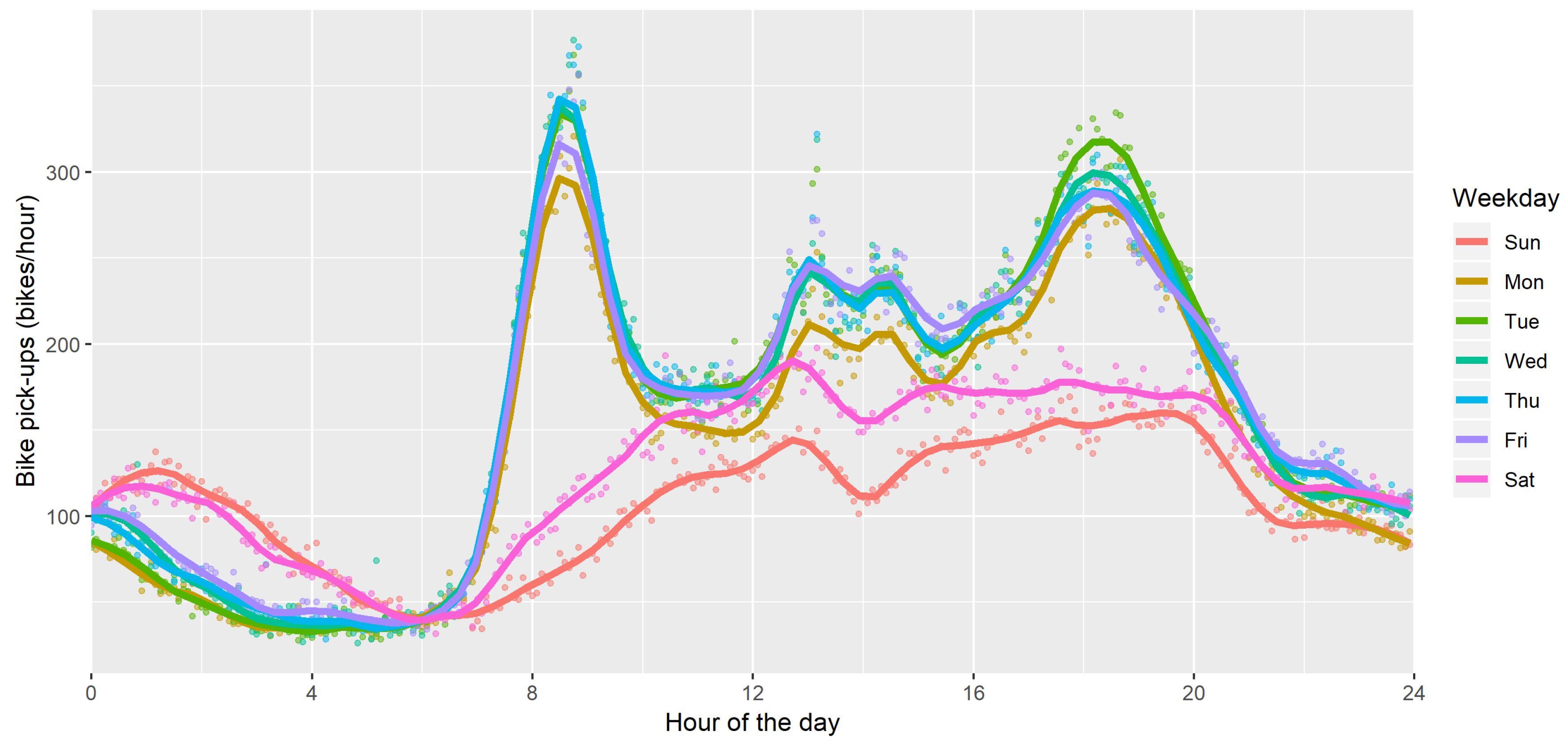
Similar trends appear on bike sharing demand patterns. Figure 5 reports the average bike pickups based on the day of the week, with a clear difference between working days and weekends. As previously described for vehicles, each point represents the median value of the bike pick-ups, grouped by the 5 min time interval and the day of the week. This aggregation allows focusing on the variability related to the particular weekday, which is graphically represented by the fitting lines of each working day.
In this case, the demand pattern of Monday appears slightly lower than the others weekdays. Another interesting remark is that while the morning and evening peaks are very similar to those related to vehicle traffic (see Figure 2), an additional double peak appears in the early afternoon, and it may be related to lunch break. This is not happening during Saturday and Sunday.
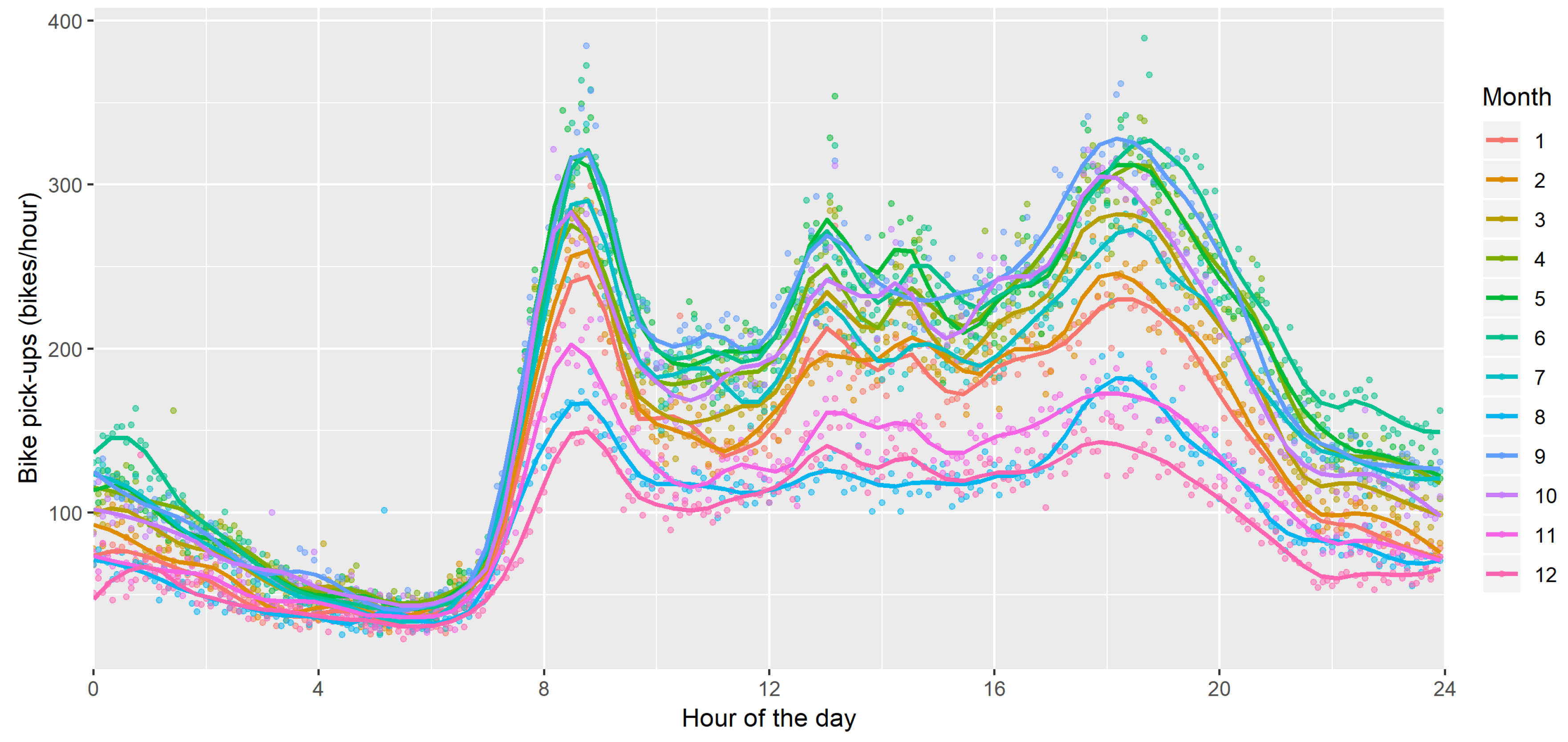
The seasonal variation is stronger for bike-sharing: the data of Figure 6 clearly highlight that users prefer bike during spring and summer, except for August, where the holidays significantly decrease the number of users. However, while the number of trips decreases across the months, the profiles remain similar, and thus the bike usage and its drivers appear to be comparable across seasons.
3.3. Potential Applications
The two datasets collected in this research work provide a comparison of the usage of bicycles and cars in an Italian city. We believe that the usage profile, if properly normalized, can be extended to other similar cities and be a basis for any activity where a high-resolution demand profile is required. Some applications may include mobility and energy planning, usage and optimization of road infrastructures, vehicles and bike use over day and year, etc.
A specific application of interest may be related to the utilization profiles of vehicles to be combined with an increasing penetration of electric vehicles (EVs). One of the main aspects in EVs adoption is related to charging profiles that will need to be possibly matched with power generation from renewables. These charging profiles are currently object of a number of research works, and they are related to the vehicles use profiles.
4. Conclusions
This research work presents two datasets that include demand profiles related to vehicles (mainly cars) and bike usage (from bike-sharing network) in the city of Turin, roughly 1 M people, in the North–West of Italy.
These datasets provide high-resolution time profiles (every five minutes) over the year 2018, allowing us to perform interesting analysis on different aspects. This paper presents the main trends for both cars and bikes, by analyzing the pattern variations within a week (working days vs weekends) and between months (being seasonality more significant for bikes than for cars).
Although these data were collected in a single city, they can be applied to similar contexts, when properly normalized. The additional value is the possibility of representing a sample distribution of mobility demand based on real values, to be applied to known figures on monthly or annual basis, which is often missing in any preliminary analysis in planning activities.
Some possible applications include calibration procedures or validation of already existing transport models related to Turin or other similar cities as long as they can be assimilated to the one analyzed. Moreover, knowing the car flows, in presence of mobility planning models, the impact of autonomous driving or increased usage of public transport can be assessed. In general, data can feed models that are able to give very practical suggestions regarding transport policies.
A future outcome of this research work may be the implementation of a web interface to constantly update the historical time series by including the most recent data available online. The availability of a larger amount of data may provide further information on the possible evolution of mobility patterns in the urban context.
Supplementary Materials
The datasets are available online at https://www.mdpi.com/2306-5729/4/3/108/s1.
Author Contributions
Conceptualization, M.N., G.C. and F.D.S.; data curation, G.C.; formal analysis, M.N.; methodology, M.N., G.C. and F.D.S.; visualization, M.N. and G.C.; writing—original draft, M.N., G.C., F.D.S. and E.C.; writing—review and editing, M.N., F.D.S. and E.C.
Funding
This research received no external funding.
Conflicts of Interest
The authors declare no conflict of interest.
References
- International Energy Agency. World Energy Outlook 2017. Available online: https://www.iea.org (accessed on 15 June 2019).
- International Transport Forum. ITF Transport Outlook 2017. Available online: https://www.itf-oecd.org (accessed on 15 June 2019).
- Gota, S.; Huizenga, C.; Peet, K.; Medimorec, N.; Bakker, S. Decarbonising transport to achieve Paris Agreement targets. Energy Effic. 2019, 12, 363–386. [Google Scholar] [CrossRef]
- Veryard, D.; Perkins, S.; Aguilar-Jaber, A.; Samsonova, T. Integrating Urban Public Transport Systems and Cycling; ITF/OECD: Paris, France, 2017. [Google Scholar]
- Lazarus, J.; Shaheen, S.; Young, S.E.; Fagnant, D.; Voege, T.; Baumgardner, W.; Fishelson, J.; Lott, J.S. Shared Automated Mobility and Public Transport; Springer International Publishing: Basel, Switzerland, 2018; pp. 142–160. [Google Scholar]
- Erhardt, G.D.; Roy, S.; Cooper, D.; Sana, B.; Chen, M.; Castiglione, J. Do transportation network companies decrease or increase congestion? Sci. Adv. 2019, 5, eaau2670. [Google Scholar] [CrossRef] [PubMed] [Green Version]
- Noussan, M. Effects of the Digital Transition in Passenger Transport—An Analysis of Energy Consumption Scenarios in Europe. FEEM Work. Pap. 2019, 2019-01. [Google Scholar] [CrossRef]
- Kay, W.A.; Andreas, H.; Kai, N. The Multi-Agent Transport Simulation MATSim; Ubiquity Press: London, UK, 2016. [Google Scholar]
- Luis Miguel Martinez, J.M.V. Assessing the impacts of deploying a shared self-driving urban mobility system: An agent-based model applied to the city of Lisbon, Portugal. Int. J. Transp. Technol. 2017, 6, 13–27. [Google Scholar] [CrossRef]
- Haasz, T.; Vilchez, J.J.G.; Kunze, R.; Deane, P.; Fraboulet, D.; Fahl, U.; Mulholland, E. Perspectives on decarbonizing the transport sector in the EU-28. Energy Strategy Rev. 2018, 20, 124–132. [Google Scholar] [CrossRef]
- International Energy Agency. World Energy Outlook 2018. Available online: https://www.iea.org (accessed on 15 June 2019).
- Salvucci, R.; Tattini, J.; Gargiulo, M.; Lehtila, A.; Karlsson, K. Modelling transport modal shift in TIMES models through elasticities of substitutions. Appl. Energy 2018, 232, 740–751. [Google Scholar] [CrossRef]
- Tattini, J.; Gargiulo, M.; Karlsson, K. Reaching carbon neutral transport sector in Denmark—Evidence from the incorporation of modal shift into the TIMES energy system modeling framework. Energy Policy 2018, 113, 571–583. [Google Scholar] [CrossRef]
- Lazarus, J.; Shaheen, S.; Young, S.E.; Fagnant, D.; Voege, T.; Baumgardner, W.; Fishelson, J.; Lott, J.S. Detailed assessment of global transport-energy models’ structures and projections. Transp. Res. Part D 2016, 55, 294–309. [Google Scholar] [CrossRef]
- Andersen, F.M.; Larsen, H.V.; Boomsmab, T.K. Long-term forecasting of hourly electricity load: Identification of consumption profiles and segmentation of customers. Energy Convers. Manag. 2013, 68, 244–252. [Google Scholar] [CrossRef]
- Zhang, F.; Wu, L.; Zhu, D.; Liu, Y. Social sensing from street-level imagery: A case study in learning spatio-temporal urban mobility patterns. ISPRS J. Photogramm. Remote. Sens. 2019, 153, 48–58. [Google Scholar] [CrossRef]
- Jelica, D.; Taljegard, M.; Thorson, L.; Johnsson, F. Hourly electricity demand from an electric road system—A Swedish case study. Appl. Energy 2018, 228, 141–148. [Google Scholar] [CrossRef]
- Sekuła, P.; Marković, N.; Laan, Z.V.; Sadabadi, K.F. Estimating Historical Hourly Trac Volumes via Machine Learning and Vehicle Probe Data: A Maryland Case Study. arXiv, 2017; arXiv:1711.00721. [Google Scholar]
- Regional Integrated Transportation Information System (RITIS). 2016. Available online: www.cattlab.umd.edu/?portfolio=ritis (accessed on 10 June 2019).
- The Study on Integrated Urban Transportation Master Plan for Istanbul Metropolitan Area in the Republic of Turkey. 2006. Available online: http://openjicareport.jica.go.jp/pdf/1196572003.pdf (accessed on 10 June 2019).
- Oppermann, M.; Möller, T.; Sedlmair, M. Bike Sharing Atlas: Visual Analysis of Bike-Sharing Networks. Int. J. Transp. 2018, 6, 1–14. [Google Scholar] [CrossRef]
- Levy, N.; Golani, C.; Ben-Elia, E. An exploratory study of spatial patterns of cycling in Tel Aviv using passively generated bike-sharing data. J. Transp. Geogr. 2019, 76, 325–334. [Google Scholar] [CrossRef]
- Kou, Z.; Cai, H. Understanding bike sharing travel patterns: An analysis of trip data from eight cities. Phys. A 2019, 515, 785–797. [Google Scholar] [CrossRef]
- Ashqar, H.I.; Elhenawy, M.; Rakha, H.A. Modeling bike counts in a bike-sharing system considering the effect of weather conditions. Case Stud. Transp. Policy 2019, 7, 261–268. [Google Scholar] [CrossRef]
- McKenzie, G. Spatiotemporal comparative analysis of scooter-share and bike-share usage patterns in Washington, D.C. J. Transp. Geogr. 2019, 78, 19–28. [Google Scholar] [CrossRef]
- Jestico, B.; Nelson, T.; Winters, M. Mapping ridership using crowdsourced cycling data. J. Transp. Geogr. 2016, 52, 90–97. [Google Scholar] [CrossRef] [Green Version]
- Safety through Disruption (Safe-D) National University Transportation Center. Vehicle Operating Speed on Urban Arterial Roadways. 2019. Available online: www.cattlab.umd.edu/?portfolio=ritis (accessed on 10 June 2019).
- SANDAG. San Diego Regional Bike and Pedestrian Counters. 2019. Available online: http://www.eco-public.com/ParcPublic/?id=681 (accessed on 10 June 2019).
- CENSIS-ANIASA. L’Evoluzione Della Mobilità degli Italiani—Dallo Scenario Attuale al 2020–2030. Technical Report. 2015. (In Italian). Available online: https://www.aniasa.it/aniasa/aniasa-informa/public/pubblicazioni/2081 (accessed on 10 June 2019).
- 5T. Opendata 5T. 2019. Available online: http://opendata.5t.torino.it/getunderlinetag|fdt (accessed on 10 June 2019).
- Solez, I.P. Study on Specific Supply Chains in Professional Urban Freight Transport and Delivery Services. 2007. Available online: https://www.interreg-central.eu/Content.Node/SOLEZ/DT221-Study-on-urban-freight-transport.pdf (accessed on 10 June 2019).
- Italian Open Data Licence. 2019. Available online: https://www.dati.gov.it/content/italian-open-data-license-v20 (accessed on 10 June 2019).
- TObike. TObike Website—Stations. 2019. Available online: http://www.tobike.it/frmLeStazioni.aspx (accessed on 10 June 2019).
- Agenzia della Mobilità Piemontese. Approfondimento sull’uso della Bicicletta e del Servizio di Bikesharing a Torino; Technical Report; AMP: Turin, Italy, 2016. (In Italian) [Google Scholar]
- R Core Team. R: A Language and Environment for Statistical Computing; R Foundation for Statistical Computing: Vienna, Austria, 2018. [Google Scholar]
- Wickham, H. Tidyverse: Easily Install and Load the ’Tidyverse’, R Package Version 1.2.1; 2017. Available online: https://tidyverse.tidyverse.org/ (accessed on 10 June 2019).
Figure 1.
Distribution of the number of accurate sensors for each measurement.

Figure 2.
Median vehicle flow depending on the working day (five minute data for 2018).

Figure 3.
Median vehicle flow depending on the month of the year (working days only, five minute data for 2018).
Figure 3.
Median vehicle flow depending on the month of the year (working days only, five minute data for 2018).

Figure 4.
Median vehicle speed depending on the working day (five minute data for 2018).

Figure 5.
Average bike pickups depending on the working day (five minute data for 2018).

Figure 6.
Average bike pickups depending on the working day (5-min data for 2018).

© 2019 by the authors. Licensee MDPI, Basel, Switzerland. This article is an open access article distributed under the terms and conditions of the Creative Commons Attribution (CC BY) license (http://creativecommons.org/licenses/by/4.0/).
Share and Cite
MDPI and ACS Style
Noussan, M.; Carioni, G.; Sanvito, F.D.; Colombo, E. Urban Mobility Demand Profiles: Time Series for Cars and Bike-Sharing Use as a Resource for Transport and Energy Modeling. Data 2019, 4, 108. https://doi.org/10.3390/data4030108
AMA Style
Noussan M, Carioni G, Sanvito FD, Colombo E. Urban Mobility Demand Profiles: Time Series for Cars and Bike-Sharing Use as a Resource for Transport and Energy Modeling. Data. 2019; 4(3):108. https://doi.org/10.3390/data4030108
Chicago/Turabian StyleNoussan, Michel, Giovanni Carioni, Francesco Davide Sanvito, and Emanuela Colombo. 2019. "Urban Mobility Demand Profiles: Time Series for Cars and Bike-Sharing Use as a Resource for Transport and Energy Modeling" Data 4, no. 3: 108. https://doi.org/10.3390/data4030108