All articles published by MDPI are made immediately available worldwide under an open access license. No special
permission is required to reuse all or part of the article published by MDPI, including figures and tables. For
articles published under an open access Creative Common CC BY license, any part of the article may be reused without
permission provided that the original article is clearly cited. For more information, please refer to
https://www.mdpi.com/openaccess.
Feature papers represent the most advanced research with significant potential for high impact in the field. A Feature
Paper should be a substantial original Article that involves several techniques or approaches, provides an outlook for
future research directions and describes possible research applications.
Feature papers are submitted upon individual invitation or recommendation by the scientific editors and must receive
positive feedback from the reviewers.
Editor’s Choice articles are based on recommendations by the scientific editors of MDPI journals from around the world.
Editors select a small number of articles recently published in the journal that they believe will be particularly
interesting to readers, or important in the respective research area. The aim is to provide a snapshot of some of the
most exciting work published in the various research areas of the journal.
The application of the Maximum Entropy (ME) principle leads to a minimum of the Mutual Information (MI), I(X,Y), between random variables X,Y, which is compatible with prescribed joint expectations and given ME marginal distributions. A sequence of sets of joint constraints leads to a hierarchy of lower MI bounds increasingly approaching the true MI. In particular, using standard bivariate Gaussian marginal distributions, it allows for the MI decomposition into two positive terms: the Gaussian MI (Ig), depending upon the Gaussian correlation or the correlation between ‘Gaussianized variables’, and a non‑Gaussian MI (Ing), coinciding with joint negentropy and depending upon nonlinear correlations. Joint moments of a prescribed total order p are bounded within a compact set defined by Schwarz-like inequalities, where Ing grows from zero at the ‘Gaussian manifold’ where moments are those of Gaussian distributions, towards infinity at the set’s boundary where a deterministic relationship holds. Sources of joint non-Gaussianity have been systematized by estimating Ing between the input and output from a nonlinear synthetic channel contaminated by multiplicative and non-Gaussian additive noises for a full range of signal-to-noise ratio (snr) variances. We have studied the effect of varying snr on Ig and Ing under several signal/noise scenarios.
One of the most commonly used information theoretic measures is the mutual information (MI) [1], measuring the total amount of probabilistic dependence among random variables (RVs)—see [2] for a unifying perspective and axiomatic review. MI is a positive quantity vanishing iff RVs are independent.
MI is an effective tool for multiple purposes, namely and among others: (a) Blind signal separation [3] and Independent Component Analysis (ICA) [4], both of which look for transformed and/or lagged stochastic time series [5] which minimize MI; (b) Predictability studies, Predictable Component Analysis [6] and Forecast Utility [7], all of which are focused on the analysis and decomposition of the MI between probabilistic forecasts and observed states.
Analytical expressions of MI are known for a few number of parametric joint distributions [8,9]. Alternatively, it can be numerically estimated by different methods, such as Maximum Likelihood estimators, Edgeworth expansion, Bayesian methods, equiprobable and equidistant histograms, kernel‑based probability distribution functions (PDFs), K-nearest neighbors technique—see [10,11] and references therein for a survey of estimation methods and scoring comparison studies.
In the bivariate case, treated here, the MI
, between RVs
is the Kullback–Leibler (KL) divergence:
, between the joint probability function
and the product of marginal probability distributions
where
is the expectation operator over the measure
. The MI is invariant for smooth invertible transformations of
.
The goal is the determination of theoretical lower MI bounds under certain conditions or, in other words, the minimum mutual information (MinMI) [12] between two RVs
, consistent, both with imposed marginal distributions and cross-expectations assessing their linear and nonlinear covariability. Those lower bounds can be obtained due to the application of the Maximum Entropy (ME) method to distributions [13] and to the inequality:
. Here,
is a Maximum Entropy probability distribution (MEPD) with respect to q, say
, where Ω is a PDF class verifying a given set of constraints [1]. Therefore, by using the joint MEPD
and
, the lower MI bound is obtained:
. Finding of the bivariate
is straightforward if the marginal distributions are themselves well defined ME distributions. We solve that by transforming the single variables
into others with imposed ME probability mass distributions through the so called ME-anamorphoses [14].
The joint ME probability distribution
is derived from the minimum of a functional in terms of a certain number of Lagrange parameters. The properties of multivariate ME distributions have been studied for various ME constraints, namely: (a) imposed marginals and covariance matrix [15]; (b) generic joint moments [16]. Abramov [17,18,19] has developed efficient and stable numerical iterative algorithms for computing ME distributions forced by sets of polynomial expectations. Here we use a bivariate version of the algorithm of [20], already tested in [21].
By taking a sequence of encapsulated sets of joint ME constraints we obtain an increasing hierarchy of lower MI bounds converging towards the total MI.
We particularize this methodology to the case where
are standard Gaussians, issued from single homeomorphisms of an original pair of variables
by Gaussian anamorphosis [14]. Then we get the MI
, which is decomposed into two generic positive quantities, a Gaussian MI Ig and a non-Gaussian MI Ing [21], vanishing under bivariate Gaussianty. The Gaussian MI is given by
, where
is the Pearson linear correlation between the Gaussianized variables. As for the non-Gaussian MI term Ing it relies upon imposed nonlinear correlations between the single Gaussian variables. The MI reduces to
when only moments of order one and two are imposed as ME constraints. We will note that, for certain extreme non-Gaussian marginals,
, thus showing that
[22] is not a proper MI lower bound in general.
The correlation
, hereafter called Gaussian correlation [21] is a nonlinear concordance measure like the Spearman rank correlation [23] and the Kendall τ, which, by definition are invariant for monotonically growing smooth marginal transformations. These measures have the good property of being expressed as functionals of the copula density functions [24], uniquely dependent on the cross dependency between variables.
The non-Gaussian MI ng holds some interesting characteristics. It coincides with the joint negentropy (deficit of entropy with respect to that of the Gaussian PDF with the same mean, variance and covariance) in the space of ‘Gaussianized’ variables, which is invariant for any orthogonal or oblique rotation of them. In particular for uncorrelated rotated variables, it coincides with the ‘compactness’, which measures the concentration of the joint distribution around a lower-dimensional manifold [25] which is given by
, i.e., the KL divergence with respect to the spherical Gaussian
(Gaussian with an isotropic covariance matrix with the same trace as that of
, say the total variance).
We also show that Ing comprises a series of positive terms associated to a p-sequence of imposed monomial expectations of total even order p (2,4,6,8…). The higher the number of independent constraints, the higher the order of terms that are retained in that series and the more information is extracted from the joint PDF.
We have shown that the possible values of the cross-expectations lie within a bounded set obtained by Schwarz-like inequalities. We illustrate the range of Ing values within those sets as function of third and fourth-order cross moments. Near the set’s boundary, Ing tends to infinity where a deterministic relationship holds and the ME problem functional is ill-conditioned.
In order to better understand the possible sources of joint non-Gaussianity and non-Gaussian MI, we have used the preceding method for computing Ig and Ing between the input and the output of a nonlinear channel contaminated by multiplicative and non-Gaussian noise for a full range of the signal-to-noise (snr) variance ratio. We put in evidence that sources of non-Gaussian MI arise from the nonlinearity of the transfer function, multiplicative noise and additive non-Gaussian noise [26].
Many of the results of the paper are straightforwardly generalized to the multivariate case with three or more random variables.
The paper is then organized as follows: Section 2 formalizes the Minimum Mutual Information (MinMI) principle from maximum entropy distributions, while Section 3 particularizes that principle to the MI decomposition into Gaussian and non-Gaussian MI parts. Section 4 addresses the non‑Gaussianity in a nonlinear non-Gaussian channel. The paper ends with conclusions and appendices with theoretical proofs and the numerical algorithm for solving the ME problem. This paper is followed by a companion one [27] on the estimation of non-Gaussian MI from finite samples with practical applications.
2. MI Estimation from Maximum Entropy PDFs
In this section we present the basis of the MI estimation between bivariate RVs, through the use of joint PDFs inferred by the maximum entropy (ME) method (ME-PDFs for short) in the space of transformed (anamorphed) marginals into specified ME distributions. We start with preliminary general concepts and definitions.
2.1. General Properties of Bivariate Mutual Information
Let
be continuous RVs with support given by the Cartesian product
, and let the joint PDF
be taken absolutely continuous with respect to the product of the marginal PDFs
and
. The mutual information (in nat) between
and
is a non-negative real functional of
expressed in different equivalent forms as:
in terms both of a KL divergence and Shannon entropies. The MI equals zero iff the RVs
and
are statistically independent, i.e., iff , except possibly in a zero‑measure set in
. Under quite general regularity conditions of PDFs, statistical independence of
and
is equivalent to the vanishing of the Pearson correlation between any pair of linear and/or nonlinear mapping functions
and
. Then, linearly uncorrelated non-independent variables have at least a non-zero nonlinear correlation. The MI between transformed variables
and
, differentiable almost everywhere, satisfies the ‘data processing inequality’
[1] with equality occurring if both
and
are smooth homeomorphisms of
and
respectively.
2.2. Congruency between Information Moment Sets
Definition 1: Following the notation of [28], we define the moment class
of bivariate PDFs
of
, as:
where
is the ρ-expectation operator,
is a J-dimensional vector composed of J absolutely
integrable functions with respect to ρXY, and
is the vector of function expectations of
. Here and henceforth,
is denoted as an information moment set.
The PDF
that maximizes the Shannon entropy or the ME-PDF verifying the constraints associated to
, hereby represented by
, must exist since
is a concave function in the non-empty convex set
. The form and estimation of the ME-PDF is described in Appendix 1. The ME-PDF satisfies the following Lemma [1]:
Lemma 1: Given two information encapsulated information moment sets:
i.e., with
including more constraining functions than
, the respective ME-PDFs
, if they exist, satisfy the following conditions:
This means that any ME-PDF log-mean is unchanged when it is computed with respect to a more constraining ME-PDF. As a corollary we have
, i.e., the ME decreases with the increasing number of constraints. This can be understood bearing in mind that the entropy maximization is performed in a more reduced PDF class, since
.
Definition 2: If two information moment sets
,
are related by linear affine relationships, then the sets are referred to as “congruent”, a property hereby denoted as
, and consequently both PDF sets are equal, i.e.,
[15]. A stronger condition than ‘congruency’ is the ME-congruency, denoted as
, holding when both the associated ME-PDFs are equal. For example, both the univariate constraint sets
and
for
lead to the same ME-PDF, the standard Gaussian N(0,1). Consequently both information moment sets are ME-congruent but not congruent since
. This is because the Lagrange multiplier of the ME functional (see Appendix 1) corresponding to the fourth moment is set to zero without any constraining effect. The congruency implies ME-congruency but not the converse.
2.3. MI Estimation from Maximum Entropy Anamorphoses
We are looking for a method of obtaining lower bound MI estimates from ME-PDFs. For that purpose we will decompose the information moment set as:
, say into a marginal or independent part
of single X and Y independent moments on
, and a cross part
on
, made by moments of joint
functions not expressible as sums of single moments. For example, by taking
,
and
for
leads to a ME-PDF which is the bivariate Gaussian with correlation
and standard Gaussians as marginal distributions.
The joint ME-PDF associated to the independent part
is the product of two independent ME-PDFs related to
and
, with the joint entropy being the sum of marginal maximum entropies, as in the case of independent random variables [15]. The KL divergence between the ME-PDFs associated to
and those associated to
is a proper MI lower bound or, expressed in other terms, a constrained mutual information. We denote it as:
Its difference with respect to
is given by:
which can be negative. However, the positiveness is ensured when marginal distributions are set to the ME-PDFs constrained by
and, which results in KL divergences vanishing with respect to the marginal PDFs in Equation (5). This procedure is quite general because
can appropriately be obtained through an injective smooth maps
from an original pair of RVs
preserving the MI, i.e.,
. Those maps are monotonically growing homeomorphisms, the hereby called ME-anamorphoses, which are obtained by equaling mass probability functions of the original variable
to those of the transformed variable
(equally for
and
) as:
The moments in
are invariant under the transformation,
, i.e., they are the same for both original and transformed variables:
(idem for
). Therefore, in the space of ME-anamorphed variables the ME-based MI (4) gives the minimum MI (MinMI), compatible with the cross moments
.
Thanks to Lemma 1, a hierarchy of ME-based MI bounds is obtainable by considering successive supersets of the ME constraints on the ME-anamorphed variables, which is justified by the theorem below.
Theorem 1: Let
be a pair of single random variables (RVs), distributed as the ME-PDF associated to the independent constraints
. Both variables can be obtained from previous ME-anamophosis. Let
be a subset of
, i.e.,
and
, such that all independent moment sets are ME-congruent (see Definition 2), i.e.,
, i.e., such that the independent extra moments in
are not further constraining the ME-PDF. Each marginal moment set is decomposed as
. For simplicity of notation, let us denote
. Then, the following inequalities between constrained mutual informations hold:
The proof is given in Appendix 2. The Theorem 1 justifies the possibility of building a monotonically growing sequence of lower bounds of
from encapsulated sequences of cross-constraints
and independent constraints
. In the sequence, the entropy associated to independent constraint sets is always constant due to the ME-congruency, while the entropy of the joint ME-PDF decreases, thus allowing the MinMIs to grow. Therefore,
is the part of MI due to cross moments in
and the positive difference
is the increment of MI due to the additional cross moments in
, while marginals are kept as preset ME-PDFs (e.g., Gaussian, Gamma, Weibull).
3. MI Decomposition under Gaussian Marginals
3.1. Gaussian Anamorphosis and Gaussian Correlation
In this section we explain how to implement the sequence of MI estimators detailed in Section 2.3 for the particular case where
and
are standard Gaussian RVs. Our aim is to estimate the MI between two original variables
of null mean and unit variance with real support. Those variables are then transformed through a homeomorphism, the Gaussian anamorphosis [14], into standard Gaussian RVs, respectively
and
, given by:
where Φ is the mass distribution function for the standard Gaussian. If
are marginally non‑Gaussian, then the Gaussian anamorphoses are nonlinear transformations. In practice, Gaussian anamorphoses can be approximated empirically from finite data sets by equaling cumulated histograms. However, for certain cases, it is analytically possible to construct bivariate distributions with specific marginal distributions and the knowledge of the joint cumulative distribution function [29].
In the case of Gaussian anamorphosis, the information moment set
of Theorem 1 includes the first and second independent moments of each variable:
. Then, following the proposed procedure of Section 2.3, we will consider a sequence of cross-constraint sets for determining the hierarchy of lower MI bounds.
The most obvious cross moment to be considered is the
expectation, equal to the Gaussian correlation
between the ‘Gaussianized’ variables
. The difference between
and the linear correlation
is easily expressed as:
The signal of the factor
in Equation (9) roughly depends on the skewness
and excess of kurtosis
through the rule of thumb, stating that
is approximated by
and
, respectively for a skewed
PDF and a symmetric
PDF (idem for
). Therefore,
can result in an enhancement of correlation
or in the opposite effect, as shown in [21] for the RV pair of meteorological variables ( = North Atlantic Oscillation Index,
= monthly precipitation). The Gaussian correlation is a concordance measure like the rank correlation and Kendall τ, being thus invariant for a monotonically growing smooth homeomorphism of both
and
. Those measures are expressed as functionals of the bivariate copula-function
, which is uniquely dependent on the cumulated marginal probabilities and equal to the density ratio, independently from the specific forms of marginal PDFs [24]. In particular, the Gaussian correlation is given by:
3.2. Gaussian and Non-Gaussian MI
The purpose of this sub-section is to express which part of MI comes from joint non-Gaussianity. If the ‘Gaussianized’ variables
are jointly non-Gaussian, then the original standardized variables
, obtained from
by invertible smooth monotonic transformations, are jointly non‑Gaussian as well. However, the converse is not true. In fact, any nonlinear transformation
of jointly Gaussian RVs
leads to non-Gaussian
with the joint non-Gaussianity arising in a trivial way. Therefore, the ‘genuine’ joint non-Gaussianity can only be diagnosed in the space of Gaussianized variables
. When the marginal PDFs of
are non-Gaussian then
in general. In particular, if the correlation
is null as it occurs when
are principal components (PCs), then
can be non-null, leading to statistically dependent PCs since they are non-linearly correlated.
The MI between Gaussianized variables
or
is expressed as
, where
is the Shannon entropy of the standard Gaussians
,
and
is the
joint entropy, associated to the joint PDF
. Given the above equality, the MI is decomposed into two positive terms:
. The first term is the Gaussian MI [21] given by
, as a function of the Gaussian correlation
(see its graphic in Figure 1), and the second one is the non-Gaussian MI
, which is due to joint non-Gaussianity and nonlinear statistical relationships among variables.
The MI
is related to the negentropy
, i.e., to the KL divergence between the PDF and the Gaussian PDF with the same moments of order one and two. That is shown by:
Theorem 2: Given
, a pair of rotated standardized variables (A being an invertible 2 × 2 matrix), one has the following result with proof in Appendix 2:
A simple consequence is that in the space of uncorrelated variables (i.e.,
), the joint negentropy is the sum of marginal negentropies with the MI, thus showing that there are intrinsic and joint sources of non-Gaussianity. One interesting corollary is derived from that.
Corollary 1: For standard Gaussian variables
and standardized rotated ones, we have
For the proof it suffices to consider Gaussian variables
in (11). Their self-negentropy vanishes by definition and the correlation term is the Gaussian MI.
Negentropy has the property of being invariant for any orthogonal or oblique rotations of the Gaussianized variables
. However, this invariance does not extend to
. From (12), in particular when
are uncorrelated (e.g., standardized principal components of
or uncorrelated standardized linear regression residuals), the negentropy equals the KL divergence between the joint PDF and that of an isotropic Gaussian with the same total variance. That KL divergence is the compactness (level of concentration around a lower-dimensional manifold), as defined in [25]. This measure is invariant under orthogonal rotations. The last term of (12) vanishes due the fact that the null correlation allows one to decompose of
into positive contributions: the self-negentropies of uncorrelated variables
and their MI
. These variables can be ‘Gaussianized’ and rotated, leading to further decomposition of
until the possible “emptying”/depletion of the initial joint non-Gaussianity into Gaussian MIs and univariate negentropies. The PDF of the new rotated variables will be closer to an isotropic spherical Gaussian PDF. Since it is algorithmically easier to compute univariate rather than multivariate entropies, the above method can be used for an efficient estimation of MIs.
The search for rotated variables maximizing the sum of individual negentropies
in (12) with minimization of
or their statistical dependency is the goal of Independent Component Analysis (ICA) [4].
A natural generalization of the MI decomposition is possible when
is obtained from a generic ME-anamorphosis by decomposing the MI into a term associated to correlation, under the constraint that marginals are set to given ME-PDFs (the equivalent to Ig), and to a term not explained by correlation (the equivalent to Ing). There is however no guarantee that this decomposition is unique as in the case of non-Gaussians, since there is no natural bivariate extension of univariate prescribed PDFs with a given correlation [30].
By looking again at Equation (12), we notice that when original variables are correlated
, the sum of marginal negentropies is not necessarily a lower bound of the joint negentropy
, because in some cases
can be negative. This means that
is not generally a proper lower bound of the MI. An example of that is given by the following discrete distribution with support on four points:
, with mass probabilities
, respectively of (1 + c)/4, (1 + c)/4, (1 − c)/4 and (1 − c)/4. This 4-point distribution has
and
zero means, unit variances and Pearson correlation
. The PDF is made of four Dirac-Deltas. In this case, the mutual information
is easily computed from the 4-point discrete mean of
while the marginal mass probabilities are
. After some lines of algebra the MI becomes:
The MI is bounded for any value of c and
as
. The graphic of
is included in Figure 1, showing that
for about
. This behavior is also reproduced by finite discontinuous PDFs (e.g., replacing the Dirac-Deltas by cylinders of probability) as well as continuous PDFs. We test it by approximating the discrete PDF by the weighted superposition of 4 spherical bivariate Gaussian PDFs, all of which have a sharp isotropic standard deviation σ = 0.001 and are centered at the 4 referred centroids. Figure 1 depicts successively growing MI lower bounds for each value of c, using the maximum entropy method (labels,
,
,
,
, see Section 3.3 for details), showing the convergence to the asymptotic value log(2).
Figure 1.
Semi-logarithmic graphs of (black thick line),
, (grey thick line) and of the successive growing estimates of
:
,
,
and
(grey thin lines). See text for details.
Figure 1.
Semi-logarithmic graphs of (black thick line),
, (grey thick line) and of the successive growing estimates of
:
,
,
and
(grey thin lines). See text for details.
3.3. The Sequence of Non-Gaussian MI Lower Bounds from Cross-Constraints
In order to build a monotonically increasing sequence of lower bounds for
(cf.Section 2.3), we have considered a sequence of encapsulated sets of functions whose moments will constrain the ME-PDFs. Those functions consist of single (univariate) and combined (bivariate) monomials of the standard Gaussians X and Y. The numerical implementation of joint ME-PDFs constrained by polynomials in dimensions d = 2, 3 and 4 was studied by Abramov [17,18,19], with particular emphasis on the efficiency and convergence of iterative algorithms. Here, we use the algorithm proposed in [21] and explained in the Appendix 1. Let us define the information moment set
as the set of bivariate monomials with total order up to p:
This set is decomposed into marginal (independent) and cross monomials as
with the corresponding vector of expectations
referring respectively to 2p and p(p − 1)/2 independent and cross moments. The components of
are of the form, where the independent part is set to the moment values of the standard Gaussian:
for an odd p and
for an even p (idem for Y), where
denotes expectation with respect to the standard Gaussian. The cross moments are bounded by a simple application of the Schwartz inequality as
. The monomials of
are linearly independent and space-generating by linear combinations, thus forming a basis in the sense of vector spaces.
For an even integer p and constraint set
there exists an integrable ME-PDF with support in
, of the form
, where
is a pth order polynomial given by a linear combination of monomials in
with weights given by Lagrange multipliers and C being a normalizing constant. That happens because
thus allowing for
as
, leading to convergence of ME-integrals [18]. For odd p, those integrals diverge because the dominant monomials
change sign from positive to negative real and therefore the ME-PDF is not well defined.
In order to build a sequence of MI lower bounds and use the procedure of Section 2.3, we have considered the sequence of information moment sets of even order
with any pair of consecutive sets satisfying the premises of Theorem 1, i.e., all independent moment sets are ME-congruent. This will lead to the corresponding monotonically growing sequence of lower bounds of MI, denoted as
, where the subscript g means that variables are marginally standard Gaussian. The first term of the sequence is the Gaussian MI
, dependent upon the Gaussian correlation. The difference between the subsequent terms and the first one leads to the non-Gaussian MI of order p defined as
, which increases with p and converges to
as
, under quite general conditions [15].
In the same manner as stated in (12), the lower bound
of
is also a lower bound for the joint negentropy, which is invariant for any affine transformations
, i.e.,
where
is the bivariate ME associated to
and
. The successive differences
are non-negative, with the extra MI being explained by moments of orders p + 1 and p + 2, while not explained by lower-order moments.
There is no analytical closed formula for the dependence of non-Gaussian MI on cross moments. However, under the scenario of low joint non-Gaussianity (small KL divergence to the joint Gaussian), the ME-PDF can be approximated by the Edgeworth expansion [31], based on orthogonal Hermite polynomials and ng approximated as a polynomial of joint bivariate cumulants:
, i + j > 2, of any pair of uncorrelated standardized variables
. Cross-cumulants are nonlinear correlations measuring joint non-Gaussianity [32], vanishing when
are jointly Gaussian. For example
is approximated as in [13] by the sum of squares:
where
is assumed to be the arithmetic average of an equivalent number neq of independent and identically distributed (iid) bivariate RVs. Therefore, from the multidimensional Central Limit Theorem [33], the larger neq is, the closer the distribution is to joint Gaussianity, and the smaller the absolute value of cumulants become.
3.4. Non-Gaussian MI across the Polytope of Cross Moments
The
cross moments in the expectation vector
(p even) are not completely free. Rather, they satisfy to Schwarz-like inequalities defining a compact set
within which cross-moments lie. That set portrays all the possible non-Gaussian ME-PDFs with p-order independent moments equal to those of the standard Gaussian. Under these conditions
. In order to have a better feel on how ng behaves, we have numerically evaluated
along the allowed set of cross-moments.
In order to determine that set, let us begin by invoking some generalities about polynomials. Any bivariate polynomial
of total order p is expressed as a linear combination of linearly independent monomials from the basis
, obtained from
including unity. Then:
If the condition
holds i.e.,
is positive semi-definite (PSD), then its expectation is non-negative:
, where
, thus imposing a constraint on the components of
. A sufficient condition for the positiveness is that
is a sum of squares (SOS) or, without loss of generality, the square of a certain polynomial
of total order p/2, where
is a column vector of coefficients multiplying monomials of
. Then,
is written as a quadratic form
. By taking the expectation operator we have
, which implies the positiveness of the matrix of moments
, which is given in terms of components of
.
When p = 4 and d = 2, the case of bivariate quartics, any PSD polynomial is a SOS [34] and vice versa. However, for p ≥ 6 there are PSD-non-SOS polynomials (e.g., those coming from the inequality between arithmetic and geometric means [35]). Therefore, a necessary and sufficient condition among fourth-order moments is that
be a PSD matrix. Let us study the conditions for that.
By ordering the set
, one has the 6 × 6 matrix
, written in the simplified form in terms of moments:
A necessary and sufficient condition for the positiveness of
is given by the application of the Sylvester criterion, stating that the determinants d1, d2, d3, d4, d5 and d6 of the 6 upper sub-matrices of
are positive. From these, only those of orders 4, 5 and 6 lead to nontrivial relationships, given with help of Mathematica® [36] as:
In Equation (22), the inequality for
has a dual relationship (d4,dual), its sign being reversed by swapping the two indices in mi,j, whereas
and
are symmetric with respect to indicial swap. The term d6 of Equation (21) is a fourth-order polynomial of cg. The inequalities for,, and hold inside a compact domain denoted D4, with the shape of what resembles a rounded polytope in the space of cross moments (), for each value of the Gaussian correlation cg. The case of Gaussianity lies within the interior of D4, corresponding to
, thus defining the hereafter called one-dimensional ‘Gaussian manifold’.
In order to illustrate how non-Gaussianity depends on moments of third and fourth order, we have computed the non-Gaussian MI of order 4 (), along a set of 2-dimensional cross-sections of D4 crossing the Gaussian manifold and extending up the boundary of D4. For Gaussian moments,
vanishes, being approximated by the Edgeworth expansion (16) near the Gaussian manifold.
In order to get a picture of
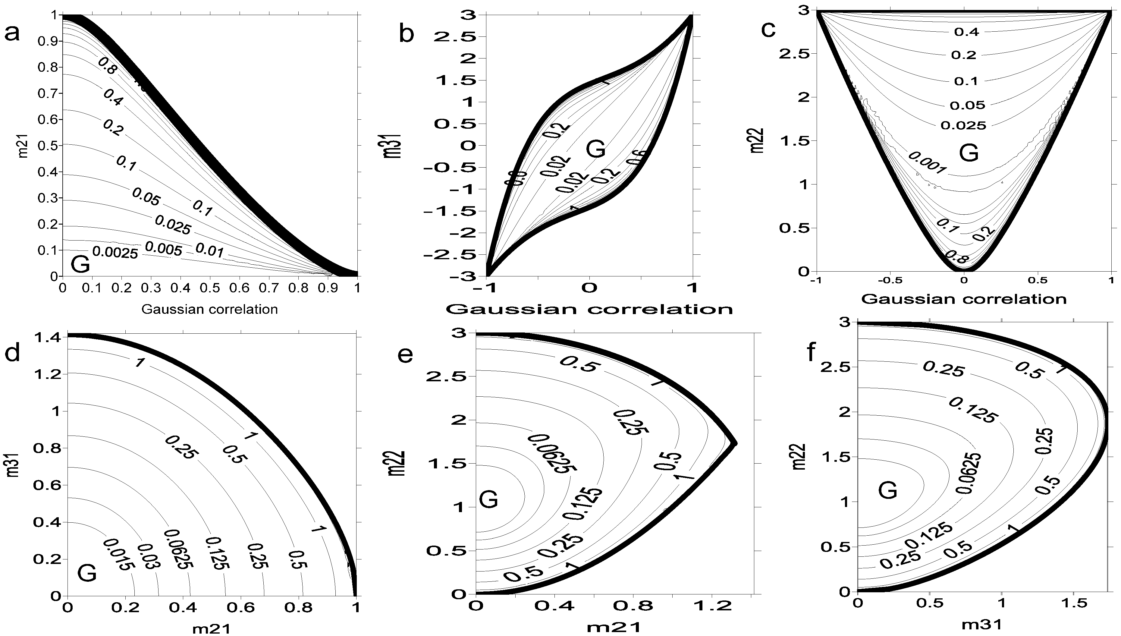
, we have chosen six particular cross-sections of D4 by varying two moments and setting the remaining to their ‘Gaussian values’. The six pairs of varying parameters are: A (cg, m2,1), B (cg, m3,1), C (cg, m2,2), D (m2,1, m3,1) at cg=0, E (m2,1, m2,2) at cg=0 and F (m3,1, m2,2) at cg= 0, with the contours of the corresponding Ing field shown in Figure 2a–f. The fields are retrieved from a discrete mesh of 100 × 100 in moment space. The Gaussian state lies at: (cg, 0), (cg, 3cg), (cg, 2cg2 + 1), (0, 0), (0, 1) and (0, 1), respectively for cases A up to F. The moment domains are obtained by solving inequalities for d4, d5 and d6 and applying the restrictions imposed by the crossing of the Gaussian manifold (e.g., m1,2= 0, m1,3= m3,1= 3cg, m2,2 = 2cg2 + 1 for case A). We obtain the following restrictions for cases A–F:
The analytical boundary of allowed domains is emphasized with thick solid lines in all Figure 2a–f. There are some common aspects among the figures. As expected, Ing vanishes at the Gaussian states, the Gaussian manifold, marked with G in Figure 2. Ing grows monotonically towards the boundary of the moment domains D4. There,
, meaning that
is singular and there is a vector
. This holds if one gets the deterministic relationship
, leading to a Dirac-Delta-like ME-PDF along a one-dimensional curve. This in turn leads to Ing = ∞, except possibly in a set of singular points of D4 on which Ing is not well defined. In practice, infinity is not reached due to stopping criteria for convergence of the iterative method used for obtaining the ME‑PDF.
Figure 2.
Field of the non-Gaussian MI
along 6 bivariate cross-sections of the set of allowed moments. Two varying moments are featured in each cross-section: A (cg, m2,1), B (cg, m3,1), C (cg, m2,2), D (m2,1, m3,1) at cg=0, E (m2,1, m2,2) at cg = 0 and F (m3,1, m2,2) at cg= 0. The letter G indicates points or curves where Gaussianity holds.
At states where |cg| = 1, Ig = ∞ and Ing has a second-kind singularity discontinuity where the contours merge together without a well-defined limit for Ing. In the neighborhood of the Gaussian state with cg = 0 in Figure 2d–f, Ing is approximated by the quadratic form (16) as is confirmed by the elliptic shape of Ing contours. The value of Ing can surpass Ig, thus emphasizing the fact that in some cases much of the MI may come from nonlinear (X,Y) correlations.
The joint entropy is invariant for a mirror symmetry in one or both variables:
or
, because the absolute value of the determinant of that transformation equals 1. As a consequence, the dependence of the Gaussian and non-Gaussian MI on moments also reflects these intrinsic mirror symmetries. For instance, in Figure 2d, the symmetry
leads to the dependency relations Ing(m2,1, m3,1) = Ing(m2,1, −m3,1), where arguments are the varying moments, while symmetry
leads to Ing(m2,1, m3,1) = Ing(−m2,1, −m3,1). The symmetries corresponding to the remaining figures are: Ing(cg, m2,1) = Ing(−cg, m2,1) = Ing(cg, −m2,1); Ing(cg, m3,1) = Ing(−cg, −m3,1); Ing(cg, m2,2) = Ing(−cg, m22); Ing(m2,1, m2,2) = Ing(−m2,1, m2,2); Ing(m3,1, m2,2) = Ing(−m3,1, m2,2), respectively for Figure 2a–c, e and f.
Near the boundary of
, the ME problem is very ill-conditioned. The Hessian matrix of the corresponding ME functional is the inverse
, where
is the covariance matrix of
, made by 8 independent plus 6 cross moments. The condition number CN (ratio between the largest and smallest eigenvalue) of
(and of
) tends to ∞ at the boundary of
where
is singular, due to the above deterministic relationship. Therefore, the closer that boundary is, the closer the ME-PDF is to a deterministic relationship, the more ill conditioned the ME problem is and the slower the numerical convergence of the optimization algorithm becomes.
4. The Effect of Noise and Nonlinearity on Non-Gaussian MI
The aim of this section is an exploratory analysis of the possible sources of non-Gaussianity in a bivariate statistical relationship. Towards that aim, we explore the qualitative behavior of Ig and Ing between a standardized signal
(with null mean and unit variance) and an
-dependent standardized response variable
contaminated by noise. For this purpose, a full range of signal-to-noise variance ratios (snr) shall be considered, from pure signal to pure noise. The statistics are evaluated from one‑million-long synthetic
iid independent realizations produced by a numeric Gaussian random generator. Many interpretations are possible for the output variable: (i)
taken as the observable outcome emerging from a noisy transmission channel fed by
(ii) given by the direct or indirect observation affected by measurement and representativeness errors corresponding to a certain value
of the model state vector [37] (iii) the outcome from a stochastic or deterministic dynamical system [38].
In order to estimate
, the working variables
are transformed by anamorphosis into standard Gaussian variables
.
We consider, without loss of generality,
. The variable
is given by Gaussian anamorphosis
as in Equation (8), with:
where
is a purely deterministic transfer function and
is a scalar noise uncorrelated with
, depending in general on
(e.g., multiplicative noise) and from a vector
of independent Gaussians contaminating the signal. Both
and
have unit variance with
. The signal-to-noise variance ratio is
.
Then, the Gaussian MI Ig is computed for each value of s∈[0,1] and compared among several scenarios of
and
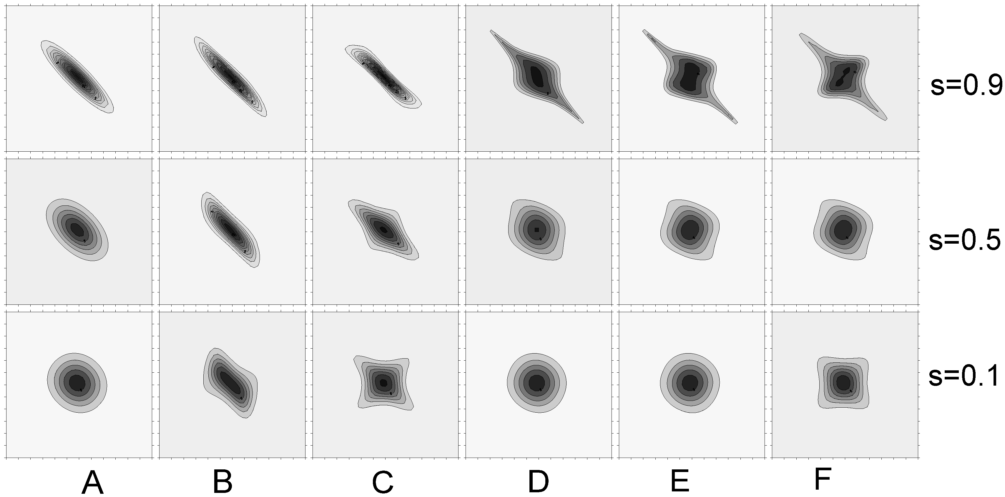
. A similar comparison is done for the non-Gaussian MI, approximated here by Ing,p=8. Six case studies have been considered (A, B, C, D, E and F); their signal and noise terms are summarized in Table 1, along with the colors with which they are represented in Figure 3 further below.
Table 1.
Types of signal and noise in Equation (35) and corresponding colors used in Figure 3.
Table 1.
Types of signal and noise in Equation (35) and corresponding colors used in Figure 3.
Case study
Color
A—Gaussian noise (reference)
Black
B—Additive non-Gaussian independent noise
Red
C—Multiplicative noise
Blue
D—Smooth nonlinear homeomorphism
Magenta
E—Smooth non-injective transformation
Green
F—Combined non-Gaussianity
Cyan
In Table 1,
are independent standard Gaussian noises. We begin with a reference case, A, which refers to Gaussian noise. Case B refers to a symmetric leptokurtic (i.e., with kurtosis larger than that of the Gaussian) non-Gaussian noise. In case C the multiplicative noise depends linearly on the signal X. In case D, the signal is a nonlinear cubic homeomorphism of the real domain. For case E, the signal is nonlinear and not injective in the interval [−1, 1], thus introducing ambiguity in the relationship
. Finally, in case F all the factors—non-Gaussian noise, multiplicative noise and signal ambiguity—are pooled together.
Figure 3.
Graphs depicting the total MI (a), Gaussian MI (b) and non-Gaussian MI (c) of order 8 for 6 cases (A–F) of different signal-noise combinations with the signal weight s in abscissas varying from 0 up to 1. See text and Table 1 for details about the cases and their color code.
Figure 3.
Graphs depicting the total MI (a), Gaussian MI (b) and non-Gaussian MI (c) of order 8 for 6 cases (A–F) of different signal-noise combinations with the signal weight s in abscissas varying from 0 up to 1. See text and Table 1 for details about the cases and their color code.
Figure 3a,b show the graphics of the total MI, estimated by Ig + Ing,8 and of the Gaussian MI (Ig) for the six cases (A to F). The graphic of non-Gaussian MI as approximated by Ing,8 is depicted in Figure 3c for five cases (B to F). In Figure 4, we show a ‘stamp-format’ collection of the contouring of ME-PDFs of polynomial order p = 8 for all cases (A to F) and extreme and intermediate cases of the snr: s = 0.1, s = 0.5 and s = 0.9. This illustrates how the snr and the nature of both the transfer function and noises influence the PDFs.
For the Gaussian noise case (A), the non-Gaussian MI is theoretically set to zero since the joint distribution of
is Gaussian. In all scenarios, both Ig and the total MI Ig + Ing grow, as expected, with the snr. This is in accordance to the Bruijn’s equality stating the positiveness of the MI derivative with respect to snr and established in the literature of signal processing for certain types of noise [39,40]. On the contrary, the monotonic behavior as a function of snr is not a universal characteristic of the non-Gaussian MI.
By observing Figure 3a–c, the following qualitative results are worth mentioning. We begin by comparing the total MI in three cases (A, B and C), which share the same linear signal but feature noise of different kinds (Figure 3a). Both the red (B) and blue (C) lines lie above the black line (A) for each given s, thus indicating that the total MI is lowest when the noise is Gaussian. This means that the Gaussian noise is the most signal degrading of noises with the same variance [41]. The extra MI found in the B and C cases come, respectively, from the Gaussian MI (see case B in Figure 3c) and from the non-Gaussian MI (see case C in Figure 3a), as it is also apparent by looking at ME-PDFs for cases B, C (s = 0.1) (Figure 4).
We consider now the cases A, D, E, all of which have a Gaussian noise. Their differences lie in the signals, with the one in A being linear and the ones in D and E being nonlinear. By comparing these cases it is seen that Ig is highest for the linear signal, the black curve lying above the magenta (D) and green (E) curves for each s in Figure 3b. This indicates that the Gaussian MI, measuring the degree of signal linearity, is lower when the signal introduces nonlinearity (cases D and E) than when no nonlinearity is present (case A).
Figure 4.
Collection of stamp-format ME-PDFs for cases A–F (see text for details) and signal weight s = 0.1 (a), s = 0.5 (b) and s = 0.9 (c) over the [−3, 3]2 support set.
Figure 4.
Collection of stamp-format ME-PDFs for cases A–F (see text for details) and signal weight s = 0.1 (a), s = 0.5 (b) and s = 0.9 (c) over the [−3, 3]2 support set.
It is worth noting that, while the signals in A and D are injective, the one in E is not, thus introducing ambiguity. This will imply loss of information in E, which is visible in the total MI depicted for each s in Figure 3a. In fact, there the green curve (case E) lies lower than the black (A) and magenta (D) curves for every s. The effect of nonlinearity is quite evident in ME-PDFs, in particular for high s value (Figure 4, cases D, E, s = 0.9).
We focus now on the non-Gaussian MI, depicted in Figure 3c for each s. The curve representing the case B, with a linear signal and a state-independent noise, indicates that the non-Gaussian MI is null for both s = 0 and s = 1. The first zero of non-Gaussian MI (at s = 0) is justified by the noise being state‑independent, whereas the second zero (at s = 1) is due to the signal being linear, which means that all the MI resides in the Gaussian MI. The non-Gaussian MI is thus positive and maximum at intermediate values of s.
By looking at case C (multiplicative noise), it is seen that the non-Gaussian MI remains roughly unchanged for every s < 1. This holds even at s = 0 (pure noise), since the noise is state-dependent and thus some information is already present. At s = 1 the non-Gaussian MI is null due to the signal being linear (as in case B).
By observing the cases with Gaussian noise and nonlinear signals (D and E) in Figure 3c, it can be seen that their non-Gaussian MI grows with s (and thus with the relative weight of the signal), due to their signals being nonlinear. This gradual behavior is also reflected in the ME-PDFs (Figure 4, cases D, E along the s values).
Finally, we consider the case in which the signal is nonlinear and the noise comprises a multiplicative and a non-Gaussian additive component (case F). As compared with E (which differs from it in that the noise is Gaussian), it can been that non-Gaussian MI is always larger in F independently of s. This is due to the fact that in F there is information even at s = 0, due to the state-dependence of its noise. For all values of s, the ME-PDF exhibits quite a large deviation from Gaussianity.
7. Discussion and Conclusions
We have addressed the problem of finding the minimum mutual information (MinMI), or the least noncommittal MI between d = 2 random variables, consistent with a set of marginal and joint expectations. The MinMI is a proper MI lower bound when marginals are set to ME-PDFs through appropriate nonlinear single anamorphoses. Moreover, the MinMI increases as long as one increases number of independent cross-constraints of the bivariate ME problem. Considering a sequence of moments, we have obtained a hierarchy of lower MI bounds approximating the total MI value. The method can easily be generalized for d > 2 variables with the necessary adaptations.
One straightforward application of that principle follows from the MI estimation from ‘Gaussianized’ variables with real support, where the marginals are rendered standard Gaussian N(0,1) by Gaussian anamorphosis. This allows for the MI decomposition into two positive contributions: a Gaussian term Ig, which depends uniquely on the Gaussian correlation cg (Pearson correlation in the space of ‘Gaussianized’ variables), and a non-Gaussian term Ing depending on nonlinear correlations. This term is equal to the joint negentropy, which is invariant for any oblique or orthogonal rotation of the ‘Gaussianized’ variables and is related to the ‘compactness’ measure or the closeness of the PDF towards a low manifold deterministic relationship. The Gaussian MI is also a ‘concordance’ measure, invariant for any monotonically growing homeomorphisms of marginals and consequently expressed as a functional of the copula-density function, which is exclusively dependent on marginal cumulated probabilities. In certain extreme cases, very far from Gaussianity, the Pearson correlation among non‑Gaussian variables is not a proper measure of the mutual information. An example of that situation is given.
Cross moments under marginal standard Gaussians are bounded by Schwarz-like inequalities defining compact sets, the shape of which resemble a rounded polytope where cross moments live. The allowed moment values portray all possible joint PDFs with Gaussian marginals. Inside that set lies the so called one-dimensional Gaussian manifold, parametrized by cg, where joint Gaussinity holds. There, Ing vanishes, growing towards infinity as far as the boundary is approached, where variables satisfy a deterministic relationship and the ME problem is ill conditioned. This behavior is illustrated in cross-sections of the polytope of cross moments of total order p = 4.
In order to systematize the possible sources of Gaussian and non-Gaussian MI, we have computed it in the context of nonlinear noisy channels. The MI has been computed between a Gaussian input and a panoply of (linear and/or nonlinear) outputs contaminated by different kinds of noise for a full range of the signal-to-noise variance ratio. Sources of non-Gaussian MI include: (a) the nonlinearity of the signal transfer function, (b) multiplicative noise and (c) non-Gaussian additive noise. This paper is followed by a companion one [27] on the estimation of non-Gaussian MI from finite samples with practical applications.
Acknowledgments
This research was developed at IDL with the financial support of project PEST-OE/CTE/LA0019/2011-FCT. Thanks are due to two anonymous reviewers, Miguel Teixeira and J. Macke for some discussions and our families for the omnipresent support.
References
Cover, T.M.; Thomas, J.A. Elements of Information Theory; John Wiley & Sons, Inc.: New York, NY, USA, 1991. [Google Scholar]
Ebrahimi, N.; Soofi, E.S.; Soyer, R. Information measures in perspective. Int. Stat. Rev.2010, 78, 383–412. [Google Scholar] [CrossRef]
Stögbauer, H.; Kraskov, A.; Astakhov, S.A.; Grassberger, P. Least-dependent-component analysis based on mutual information. Phys. Rev. E2004, 70, 066123:1–066123:17. [Google Scholar] [CrossRef]
Hyvärinen, A.; Oja, E. Independent Component Analysis: Algorithms and application. Neural Network.2000, 13, 411–430. [Google Scholar] [CrossRef]
DelSole, T. Predictability and information theory. Part I: Measures of predictability. J. Atmos. Sci.2004, 61, 2425–2440. [Google Scholar] [CrossRef]
Majda, A.; Kleeman, R.; Cai, D. A mathematical framework for quantifying predictability through relative entropy. Methods and applications of analysis. Meth. Appl. Anal.2002, 9, 425–444. [Google Scholar]
Darbellay, G.A.; Vajda, I. Entropy expressions for multivariate continuous distributions. IEEE Trans. Inform. Theor.2000, 46, 709–712. [Google Scholar] [CrossRef]
Nadarajah, S.; Zografos, K. Expressions for Rényi and Shannon entropies for bivariate distributions. Inform. Sci.2005, 170, 173–189. [Google Scholar] [CrossRef]
Khan, S.; Bandyopadhyay, S.; Ganguly, A.R.; Saigal, S.; Erickson, D.J.; Protopopescu, V.; Ostrouchov, G. Relative performance of mutual information estimation methods for quantifying the dependence among short and noisy data. Phys. Rev. E2007, 76, 026209:1–026209:15. [Google Scholar] [CrossRef]
Walters-Williams, J.; Li, Y. Estimation of mutual information: A survey. Lect. Notes Comput. Sci.2009, 5589, 389–396. [Google Scholar]
Globerson, A.; Tishby, N. The minimum information principle for discriminative learning. In Proceedings of the 20th conference on Uncertainty in artificial intelligence, Banff, Canada, 7–11 July 2004; pp. 193–200.
Jaynes, E.T. On the rationale of maximum-entropy methods. Proc. IEEE1982, 70, 939–952. [Google Scholar] [CrossRef]
Wackernagel, H. Multivariate Geostatistics—An Introduction with Applications; Springer-Verlag: Berlin, Germany, 1995. [Google Scholar]
Ebrahimi, N.; Soofi, E.S.; Soyer, R. Multivariate maximum entropy identification, transformation, and dependence. J. Multivariate Anal.2008, 99, 1217–1231. [Google Scholar] [CrossRef]
Abramov, R. An improved algorithm for the multidimensional moment-constrained maximum entropy problem. J. Comput. Phys.2007, 226, 621–644. [Google Scholar] [CrossRef]
Abramov, R. The multidimensional moment-constrained maximum entropy problem: A BFGS algorithm with constraint scaling. J. Comput. Phys.2009, 228, 96–108. [Google Scholar] [CrossRef]
Abramov, R. The multidimensional maximum entropy moment problem: A review on numerical methods. Commun. Math. Sci.2010, 8, 377–392. [Google Scholar] [CrossRef]
Rockinger, M.; Jondeau, E. Entropy densities with an application to autoregressive conditional skewness and kurtosis. J. Econometrics2002, 106, 119–142. [Google Scholar] [CrossRef]
Pires, C.A.; Perdigão, R.A.P. Non-Gaussianity and asymmetry of the winter monthly precipitation estimation from the NAO. Mon. Wea. Rev.2007, 135, 430–448. [Google Scholar] [CrossRef]
Myers, J.L.; Well, A.D. Research Design and Statistical Analysis, 2nd ed.; Lawrence Erlbaum Associates: Mahwah, NJ, USA, 2003. [Google Scholar]
Calsaverini, R.S.; Vicente, R. An information-theoretic approach to statistical dependence: Copula information. Europhys. Lett.2009, 88, 68003. 1–6. [Google Scholar] [CrossRef]
Monahan, A.H.; DelSole, T. Information theoretic measures of dependence, compactness, and non-Gaussianity for multivariate probability distributions. Nonlinear Proc. Geoph.2009, 16, 57–64. [Google Scholar] [CrossRef]
Guo, D.; Shamai, S.; Verdú, S. Mutual information and minimum mean-square error in Gaussian channels. IEEE Trans. Inform. Theor.2005, 51, 1261–1283. [Google Scholar] [CrossRef]
Pires, C.A.; Perdigão, R.A.P. Minimum mutual information and non-Gaussianity through the maximum entropy method: Estimation from finite samples. Entropy2012. submitted for publication. [Google Scholar]
Shore, J.E.; Johnson, R.W. Axiomatic derivation of the principle of maximum entropy and the principle of the minimum cross-entropy. IEEE Trans. Inform. Theor.1980, 26, 26–37. [Google Scholar] [CrossRef]
Koehler, K.J.; Symmanowski, J.T. Constructing multivariate distributions with specific marginal distributions. J. Multivariate Anal.1995, 55, 261–282. [Google Scholar] [CrossRef]
Cruz-Medina, I.R.; Osorio-Sánchez, M.; García-Páez, F. Generation of multivariate random variables with known marginal distribution and a specified correlation matrix. InterStat2010, 16, 19–29. [Google Scholar]
van Hulle, M.M. Edgeworth approximation of multivariate differential entropy. Neural Computat.2005, 17, 1903–1910. [Google Scholar] [CrossRef]
van der Vaart, A.W. Asymptotic Statistics; Cambridge University Press: New York, NY, USA, 1998. [Google Scholar]
Hilbert, D. Über die Darstellung definiter Formen als Summe von Formenquadraten. Math. Ann.1888, 32, 342–350. [Google Scholar] [CrossRef]
Ahmadi, A.A.; Parrilo, P.A. A positive definite polynomial hessian that does not factor. In Proceedings of the Joint 48th IEEE Conference on Decision and Control and 28th Chinese Control Conference, Shanghai, China, 15–18 December 2009; pp. 16–18.
Wolfram, S. The Mathematica Book, 3rd ed.; Cambridge University Press: Cambridge, UK, 1996. [Google Scholar]
Bocquet, M.; Pires, C.; Lin, W. Beyond Gaussian statistical modeling in geophysical data assimilation. Mon. Wea. Rev.2010, 138, 2997–3023. [Google Scholar] [CrossRef]
Sura, P.; Newman, M.; Penland, C.; Sardeshmuck, P. Multiplicative noise and non-Gaussianity: A paradigm for atmospheric regimes? J. Atmos. Sci.2005, 62, 1391–1406. [Google Scholar] [CrossRef]
Guo, D.; Shamai, S.; Verdú, S. Mutual information and minimum mean-square error in Gaussian channels. IEEE Trans. Inform. Theor.2005, 51, 1261–1283. [Google Scholar] [CrossRef]
Rioul, O. A simple proof of the entropy-power inequality via properties of mutual information. arXiv2007. arXiv:cs/0701050v2 [cs.IT]. [Google Scholar]
Guo, D.; Wu, Y.; Shamai, S.; Verdú, S. Estimation in gaussian noise: Properties of the minimum mean-square error. IEEE T. Inform. Theory2011, 57, 2371–2385. [Google Scholar]
Gilbert, J.; Lemaréchal, C. Some numerical experiments with variable-storage quasi-Newton algorithms. Math. Program.1989, 45, 407–435. [Google Scholar] [CrossRef]
Appendix 1 Form and Numerical Estimation of ME-PDFs
We hereby present a summary of the ME method for distributions along with the numerical algorithm for computing it. Let us consider an information moment set (2)
comprising J constraints on the RVs
with the support set
The associated ME-PDF is obtained from the absolute minimum of a control function:
in terms of a J-dimensional vector of Lagrange multipliers:
where
[13]. The minimum of
lies at a value of
dependent on
, given by:
. The corresponding L minimum is the value of the maximum entropy:
.
The ME-PDF is of the form:
, where
is the normalization partition function. Except when no analytical relationship
exists, this function has to be estimated by iterative techniques of minimization of
. The numerical algorithm consists of a bivariate version of that presented in [20]. In practice, we have solved the ME problem for a finite square support set
with r large enough in order to prevent significant boundary effects on the ME-PDF, thus obtaining a good estimation of the ME-PDF asymptotic limit when r → ∞. By using the two-dimensional Leibnitz differentiation rule, it is easy to obtain the derivative of the ME
with respect to r:
where the line integral is always positive and computed along the boundary line
of
. When |x|,|y| → ∞, the bound of (A1) leads to the scaling of the logarithm of the ME-PDF as
, where p is the maximum total order of the constraining bivariate monomials in the information moment set
. Furthermore, in order to get integrands of the order
during the optimization process, we solve the ME problem for the scaled variables (X/r,Y/r) in the square [−1, 1]2, by taking the appropriate scaled constraints. Then, we apply the scaling entropy relationship:
The integrals giving the functional
and its η-derivatives are approximated by the bivariate Gauss truncation rule with Nf weighting factors each in the interval [−1, 1]. In order to get full resolution during the minimization, and to avoid “Not-a-Number” (NAN) and infinity (INF) errors in computation, we subtract the polynomials in the arguments of exponentials from the corresponding maximum in S. Finally, the functional
is multiplied by a sufficient high factor F in order to emphasize the gradient. After some preliminary experiments, we have set r = 6, Nf = 80, F = 1000. Convergence is assumed to be reached when one gets an accuracy of 10−6 for the gradient of
. By setting the first guess of Lagrange multipliers (FGLM) to zero, convergence is reached after about 60–400 iterations. For the optimization we have used the routine M1QN3 from INRIA [42], which uses the Quasi-Newton BFGS algorithm. Convergence is slower under a higher condition number (CN) of the Hessian of
, with the convergence time growing in general with the proximity of the boundary of the domain of allowed moments as well as the total maximum order p of constraining monomials. The convergence is faster when a closer FGLM is provided to the exact solution. This is possible in sequential ME problems with quite small successive constraint differences. There, one uses a continuation technique by setting FGLM to the optimized Lagrange multipliers from the previous ME problem. This technique has been used in the computation of the graphics in Figure 3.
Appendix 2
Proof of Theorem 1: Since X follows the ME-PDF generated by
and ME-congruency holds, we have
with similar identities for Y. Therefore, the first inequality of (7a) follow directly from (5). The second one is obtained by difference and application of Lemma 1 to
(q.e.d.).
Proof of Theorem 2: The first equality of (11) comes from Equation (1) as
and from the negentropy definition of Gaussianized variables
, where
is the entropy of the Gaussian fit. From the entropy formula of transformed variables we get, leading to the negentropy equality
. Finally, the last equation of (11) comes from the equality
and the definition of negentropy, i.e.,
(q.e.d.).
Pires, C.A.L.; Perdigão, R.A.P.
Minimum Mutual Information and Non-Gaussianity Through the Maximum Entropy Method: Theory and Properties. Entropy2012, 14, 1103-1126.
https://doi.org/10.3390/e14061103
AMA Style
Pires CAL, Perdigão RAP.
Minimum Mutual Information and Non-Gaussianity Through the Maximum Entropy Method: Theory and Properties. Entropy. 2012; 14(6):1103-1126.
https://doi.org/10.3390/e14061103
Chicago/Turabian Style
Pires, Carlos A. L., and Rui A. P. Perdigão.
2012. "Minimum Mutual Information and Non-Gaussianity Through the Maximum Entropy Method: Theory and Properties" Entropy 14, no. 6: 1103-1126.
https://doi.org/10.3390/e14061103
Article Metrics
No
No
Article Access Statistics
For more information on the journal statistics, click here.
Multiple requests from the same IP address are counted as one view.
Pires, C.A.L.; Perdigão, R.A.P.
Minimum Mutual Information and Non-Gaussianity Through the Maximum Entropy Method: Theory and Properties. Entropy2012, 14, 1103-1126.
https://doi.org/10.3390/e14061103
AMA Style
Pires CAL, Perdigão RAP.
Minimum Mutual Information and Non-Gaussianity Through the Maximum Entropy Method: Theory and Properties. Entropy. 2012; 14(6):1103-1126.
https://doi.org/10.3390/e14061103
Chicago/Turabian Style
Pires, Carlos A. L., and Rui A. P. Perdigão.
2012. "Minimum Mutual Information and Non-Gaussianity Through the Maximum Entropy Method: Theory and Properties" Entropy 14, no. 6: 1103-1126.
https://doi.org/10.3390/e14061103


