Ordinal Patterns, Entropy, and EEG

Abstract

In this paper we illustrate the potential of ordinal-patterns-based methods for analysis of real-world data and, especially, of electroencephalogram (EEG) data. We apply already known (empirical permutation entropy, ordinal pattern distributions) and new (empirical conditional entropy of ordinal patterns, robust to noise empirical permutation entropy) methods for measuring complexity, segmentation and classification of time series.

1. Introduction

The investigation of data on the basis of considering ordinal pattern distributions provides a new and promising approach to time series analysis. Since the appearance of the seminal paper [1] of Bandt and Pompe inventing (empirical) permutation entropy, the number of papers describing and using this approach is rapidly increasing. In particular, empirical permutation entropy has been applied to EEG data for detecting and visualizing changes related to epileptic seizures (e.g., [2–5]), for distinguishing brain states related to anesthesia (e.g., [6,7]), for discriminating sleep stages [8], as well as for analyzing and classifying heart rate variability data (e.g., [9–12]), and in financial and physical time series analysis (see [13,14] for a review of applications).

The paper is devoted to illustrating the potential of already known and new ordinal-patterns-based methods for measuring complexity of real-world data and, especially, of EEG data. In particular, we discuss empirical permutation entropy (ePE) and two related concepts, called empirical conditional entropy of ordinal patterns (eCE) [15] and robust (to noise) empirical permutation entropy (rePE).

Here two aspects will be of special interest. At first, we compare computational and discriminatory performance of ePE and eCE with that of approximate entropy (ApEn) and sample entropy (SampEn), being common in complex data analysis. Approximate entropy has been applied in several cardiovascular studies (see for a review [16]), for quantifying the effect of anesthesia drugs on the brain activity [17–19], for discriminating sleep stages [20,21], for epileptic EEG analysis and epileptic seizures detection [22,23] and in other fields (see [24,25] for a review of applications). Applications of sample entropy have been given in several cardiovascular studies [9,26] (see for a review [16]), for analysis of EEG data from patients with Alzheimer’s disease [27], for epileptic EEG analysis and epileptic seizures detection [2,28] and other applications (see [24,25,29] for a review).

The second main aspect discussed in the paper is using ordinal patterns for the classification of EEG data, which was first suggested in [30,31]. Namely, we introduce a CEofOP (“Conditional-Entropy-of-Ordinal-Patterns-based”) statistic for finding points where a time series is qualitatively changing. The detected change-points split the time series into homogenous segments that are further clustered with respect to their ordinal pattern distributions.

The paper is organized as follows. In Section 2 we recall the concepts of approximate entropy and sample entropy and define the main concepts used in our ordinal-patterns-based approach to time series analysis including the empirical permutation entropy, the empirical conditional entropy of ordinal patterns, and the robust empirical permutation entropy. The performance of the different quantifiers is investigated and illustrated, on the one hand for simulated data from chaotic maps, which are often used in complexity research, and on the other hand for EEG data with the aim of discriminating between different states. Section 3 is devoted to ordinal-patterns-based segmentation and to the classification of the obtained segments. For this the CEofOP statistic is introduced and explained. Its performance is illustrated for the discrimination of sleep stages from EEG data. Finally, Section 4 provides a summary including conclusions with some relevance for future research.

In the whole paper, we denote by ℕ and ℝ the set of natural and real numbers, respectively.

2. Entropies for Discriminating Complexity

2.1. Approximate Entropy and Sample Entropy

We recall the approximate entropy and the sample entropy, widely used in time series analysis as practical complexity measures and originally introduced in [24,32]. We do not go into theoretical details behind the concepts, but only note that they are related to such theoretical concepts as correlation entropy [33], Eckmann–Ruelle entropy [34], Kolmogorov–Sinai entropy [35] and H₂(T)-entropy [36] (see also [37] for the discussion of their relationships).

Definition 1. Given a time series${(x_i)}_{i=1}^N$ with N ∈ ℕ, a length of compared vectors k ∈ ℕ and a tolerance r ∈ ℝ for accepting similar vectors, the approximate entropy($\text{ApEn}\left(k,r,{(x_i)}_{i=1}^N\right)$) and the sample entropy ($\text{SampEn}\left(k,r,{(x_i)}_{i=1}^N\right)$) are defined as [24,32]:

$$\begin{array}{l}\text{ApEn}\left(k,r,{(x_i)}_{i=1}^N\right)=\frac{{\displaystyle \sum {}_{i=1}^{N-k+1}\ln \widehat{C}\left(i,k,r,{(x_i)}_{i=1}^N\right)}}{N-k+1}-\frac{{\displaystyle \sum {}_{i=1}^{N-k}\ln \widehat{C}\left(i,k+1,r,{(x_i)}_{i=1}^N\right)}}{N-k+},\\ \widehat{C}\left(i,k,r,{(x_i)}_{i=1}^N\right)=\frac{1}{N-k+1}\#\left\{1\le j\le N-k+1:\underset{l=0,1,\dots ,k-1}{max}|x_{i+l}-x_{i+l}|\le r\right\},\end{array}$$

(1)

$$\begin{array}{l}\text{SampEn}(k,r,{(x_i)}_{i=1}^N)=\ln \widehat{C}(k,r,{(x_i)}_{i=1}^N)-\ln \widehat{C}(k+1,r,{(x_i)}_{i=1}^N),\hfill \\ \widehat{C}(k,r,{(x_i)}_{i=1}^N)=\frac{2}{(N-k-1)(N-k)}\#\{(i,j):1\le i<j\le N-k+1,\underset{l=0,1,\dots ,k-1}{\max }|x_{i+l}-x_{j+l}|\le r\},\hfill \end{array}$$

(2)

where #A stands for the number of elements of a set A.

Note that $\text{SampEn}\left(k,r,{(x_i)}_{i=1}^N\right)$ is undefined when either $\widehat{C}\left(k,r,{(x_i)}_{i=1}^N\right)=0$ or $\widehat{C}\left(k+1,r,{(x_i)}_{i=1}^N\right)=0$.

We use further the short form ApEn(k, r, N) and SampEn(k, r, N) instead of $\text{ApEn}\left(k,r,{(x_i)}_{i=1}^N\right)$ and $\text{SampEn}\left(k,r,{(x_i)}_{i=1}^N\right)$ when no confusion can arise.

Note that when computing ApEn by (1) one counts each vector as matching itself, because

$$\underset{l=0,1,\dots ,k-1}{max}|x_{i+l}-x_{j+l}|=0\le r$$

, which introduces some bias in the result [24]. When computing SampEn one does not count self-matches due to i < j in (2), which is more natural [24].

It holds for all k, N ∈ ℕ and r ∈ ℝ that [24]:

$$0\le \text{ApEn}\left(k,r,N\right)\le \ln (N-k),$$

(3)

$$0\le \text{SampEn}\left(k,r,N\right)\le \ln (N-k)+\ln \left(\frac{N-k-1}{2}\right).$$

(4)

For application of both entropies to real-world time series, the tolerance r is usually recommended to set to r ∈ [0.1σ, 0.25σ], where σ is the standard deviation of a time series, and the length k of compared vectors is recommended to set to k = 2 [24,32,38]. In order to compare the complexities of two time series, one has to fix k, r and N due to the significant variation of the values of $\text{ApEn}\left(k,r,{(x_i)}_{i=1}^N\right)$ and $\text{SampEn}\left(k,r,{(x_i)}_{i=1}^N\right)$ for different parameters [24,38].

2.2. Ordinal Patterns, Empirical Permutation Entropy and Empirical Conditional Entropy of Ordinal Patterns

In this subsection we define ordinal patterns, empirical permutation entropy [1] and empirical conditional entropy of ordinal patterns [15]. We start from the definition of ordinal patterns.

Definition 2. A vector (x₀, x₁,…, x_d) ∈ ℝ^d+1 has the ordinal pattern π = (r₀, r₁, …, r_d) of order d ∈ ℕ if

$$\begin{array}{l}{x}_{r_0}\ge x_{r_1}\ge \dots \ge x_{r_d},\mathit{\text{and}}\hfill \\ r_{l-1}>r_l\mathit{\text{in the case}}{x}_{r_{l-1}}=x_{r_l}.\hfill \end{array}$$

For example, all ordinal patterns of order d = 2 are given in Figure 1.

The empirical permutation entropy was originally introduced in [1] as a natural measure of time series complexity. This quantity is an estimate of the permutation entropy, which is strongly related to the well-known Kolmogorov–Sinai entropy (see for the theoretical background [13,39]).

Definition 3. By the empirical permutation entropy of order d ∈ ℕ and of delay τ ∈ ℕ of a time series${(x_i)}_{i=1}^N$ with N ∈ ℕ we understand the quantity

$$\begin{array}{l}\text{ePE}\left(d,\tau ,{(x_i)}_{i=1}^N\right)=-\frac{1}{d}{\displaystyle \sum _{j=0}^{(d+1)!-1}{p}_j\ln }{p}_j,where\\ p_j=\frac{\#\{i=d\tau +1,d\tau +2,\dots ,N|(x_i,x_{i-\tau },\dots ,x_{i-d\tau })\mathit{\text{has the ordinal pattern}}j\}}{N-d\tau }\\ (with0\ln 0:=0).\end{array}$$

Here assume that all possible ordinal patterns are enumerated by 0, 1, …, (d + 1)! − 1 [40].

We use the short form ePE(d, τ, N) instead of $\text{ePE}\left(d,\tau ,{(x_i)}_{i=1}^N\right)$ when no confusion can arise.

The empirical permutation entropy is a well-interpretable measure of complexity. Indeed, the higher the diversity of ordinal patterns of order d in a time series ${(x_i)}_{i=1}^N$ is, the larger the value of ePE(d, τ, N) is. It holds for d, N, τ ∈ ℕ:

$$0\le \text{ePE}(d,\tau ,N)\le \frac{\ln ((d+1)!)}{d},$$

(5)

which is restrictive for estimating a large complexity as we show in Example 4 in Section 2.4. The choice of order d is rather simple. The larger d is, the better the estimate of complexity underlying a system by the empirical permutation entropy is. On the other hand, excessively high d value leads to an underestimation of the complexity because by the bounded length of a time series not all ordinal patterns representing the system can occur. In [41],

$$5(d+1)!<N$$

(6)

is recommended. The choice of the delay τ is a bit complicated; in many applications τ = 1 is used, however larger delays τ can provide additional information as we illustrate in Example 5 for EEG data (see also [42] for the discussion of the choice of τ). Note also that increasing the delay τ can lead to increasing the values of ePE, i.e., when increasing the delay τ one should mind the bound (5) as we illustrate in the following example (see also [37] for more details).

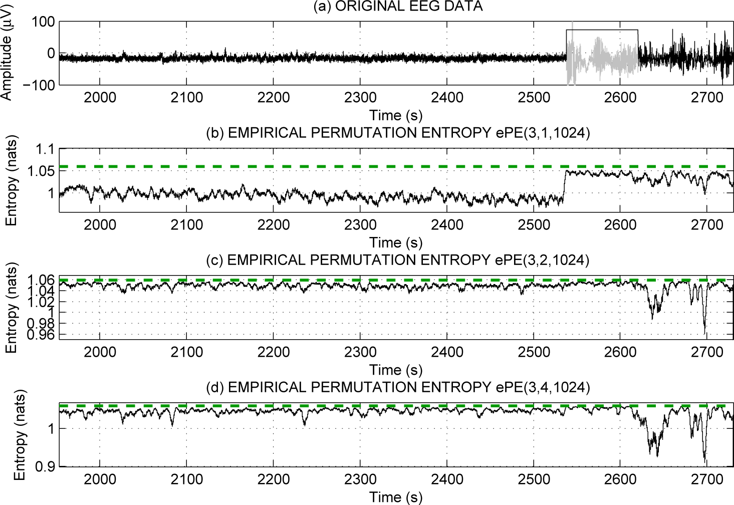
Example 1. In Figure 2 we present the values of ePE(3, τ, N) for the delays τ = 1, 2, 4 computed in sliding windows of size N = 1024 of EEG recording (from the European Epilepsy Database [44]) with the epileptic seizure marked in gray in the upper plot. The EEG is recorded from channel F4 from a female patient, 54 years old with epilepsy caused by hippocampal sclerosis, the complex partial seizure is recorded during a sleep stage S2. One can see that the values of ePE are larger for τ = 2 and τ = 4 than for τ = 1, and they almost attain the upper bound$\frac{\ln 24}{3}=1.0594$ (green dashed line). For τ = 1 the ePE values reflect the seizure by the increase of their values, whereas the ePE values for τ = 2 and τ = 4 do not reflect the seizure; they cannot increase since they are bounded by 1.0594.

Note that here the epileptic seizure is reflected by an increase of the ePE values during the epileptic seizure, in spite of many results that report decrease of ePE values during the seizure (e.g., [3,4,43]). When analyzing EEG recordings from [44] we have found out that seizures that occurred during the awake state (W) are often reflected by a decrease of ePE values, whereas seizures that occurred during the sleep stages (S1, S2, REM) are reflected by an increase of ePE values. (Note that no seizures occurred in sleep stages S3 and S4 in the database [44].) The explanation is that the ePE values during sleep are usually less than the values of ePE during the awake state; see [37] for more details.

We define now the empirical conditional entropy of ordinal patterns. The theoretical conditional entropy of ordinal patterns is introduced in [15], and for several cases it estimates the Kolmogorov-Sinai entropy better than the permutation entropy (see [15] for details and examples).

Definition 4. By the empirical conditional entropy of ordinal patterns eCE $\text{eCE}\left(d,\tau ,{(x_i)}_{i=1}^N\right)$ of order d ∈ ℕ and of delay τ ∈ ℕ of a time series${(x_i)}_{i=1}^N$ with N ∈ ℕ we understand the quantity

$$\begin{array}{l}\text{eCE}(d,\tau ,{(x_i)}_{i=1}^N)=-{\displaystyle \sum }_{j=0}^{(d+1)!-1}{\displaystyle \sum }_{l=0}^{(d+1)!-1}{p}_j{q}_{j,l}\ln q_{j,l},\mathit{\text{where}}\hfill \\ \begin{array}{l}{p}_j=\frac{\#\{i\in I|(x_i,x_{i-\tau },\dots ,x_{i-d\tau })\mathit{\text{hasordinal pattern j}}\}}{N-d\tau -\tau }\\ q_{j,l}=\frac{\#\{i\in I|(x_i,x_{i-\tau },\dots ,x_{i-d\tau })\mathit{\text{and}}(x_{i+\tau },x_i,\dots ,x_{i-(d-1)\tau })\mathit{\text{have ordinal pattern j and l}}\}}{\#\{i\in I|(x_i,x_{i-\tau },\dots ,x_{i-d\tau })\mathit{\text{has ordinal pattern j}}\}},\end{array}\hfill \\ \mathit{\text{for}}I=\{d\tau +1,d\tau +2,\dots ,N-\tau \}\hfill \\ (\mathit{\text{with}}0\ln 0:=0\mathit{\text{and}}0/0:=0).\hfill \end{array}$$

(7)

(Again assume that all possible ordinal patterns are enumerated by 0,1,…, (d + 1)! − 1.)

Further we use the short form eCE(d, τ, N) instead of $\text{eCE}\left(d,\tau ,{(x_i)}_{i=1}^N\right)$ when no confusion can arise.

The empirical conditional entropy characterizes the average diversity of ordinal patterns succeeding a given one. It holds for d, N, τ ∈ ℕ:

$$0\le \text{eCE}\left(d,\tau ,N\right)\le \ln (d+1).$$

(8)

The choice of the order d of the empirical conditional entropy is similar to that of the empirical permutation entropy. Similar to (6), order d and length N of a time series should satisfy 5(d + 1)!(d + 1) < N, otherwise eCE can be underestimated. (Note that to compute eCE one has to estimate frequencies of all possible pairs of ordinal patterns, and there are (d + 1)!(d + 1) such pairs.) However, our experience is that in many cases it is enough to have

$$(d+1)!(d+1)<N.$$

(9)

Remark 1. For further discussion let us note that the permutation entropy is equal to the well-known theoretical measure of dynamical systems complexity, the Kolmogorov–Sinai entropy, for strictly monotone piecewise interval maps due to the result from [45]. For certain cases of interval maps, in particular, for the logistic map T_LM(x) = Ax(1 − x) with A ∈ [3.5, 4] and for the tent map T_TM = A min(x, 1 − x) with A ∈ (1, 2], the Kolmogorov–Sinai entropy can be estimated by the Lyapunov exponent, which we use further in experiments (see [46,47] for the theoretical background).

2.3. Robustness of Empirical Permutation Entropy with Respect to Noise

In this subsection we discuss the robustness of the empirical permutation entropy with respect to observational noise since it is not as robust to noise as it is usually reported (e.g., [48,49]). Given a time series ${(x_i)}_{i=1}^N$, the observational noise${({\xi }_i)}_{i=1}^N$ adds an error ξ_i to each value x_i:

$$y_i=x_i+{\xi }_i.$$

We introduce the (rePE), which is based on counting robust ordinal patterns defined in the following way.

Definition 5. For positive η ∈ ℝ, let us call an ordinal pattern of the vector (x_t, x_t-τ, …, x_t-dτ) ∈ ℝ^d+1 η-robust if

$$\#\{(i,j):0\le i<j\le d,|x_{t-i\tau }-x_{t-j\tau }|<\eta \}<\frac{(d+1)d}{8}.$$

(10)

The threshold $\frac{(d+1)d}{8}$ is chosen as a quarter of the amount of the ordered pairs of entries from the vector (x_t, x_t-τ, …, x_t-dτ).

Definition 6. For positive η ∈ ℝ, by the η-robust empirical permutation entropy (rePE) of order d ∈ ℕ and of delay τ ∈ ℕ of a time series${(x_i)}_{i=1}^N$, we understand the quantity

$$\begin{array}{l}\text{rePE}\left(d,\tau ,{(x_i)}_{i=1}^N,\eta \right)=-\frac{1}{d}{\displaystyle \sum _{j=0}^{(d+1)!-1}{p}_j\ln p_j},where\\ p_j=\frac{\#\{i=d\tau +1,d\tau +2,\dots ,N|(x_i,x_{i-\tau },\dots ,x_{i-d\tau })\mathit{\text{has the}}\eta -robust\mathit{\text{ordinal pattern}}j\}}{\#\{i=d\tau +1,d\tau +2,\dots ,N|(x_i,x_{i-\tau },\dots ,x_{i-d\tau })\mathit{\text{has an}}\eta -\mathit{\text{robust ordinal pattern}}\}}\\ (with0\ln 0:=0and0/0:=0).\end{array}$$

(Again assume that all possible ordinal patterns are enumerated by 0,1,…, (d + 1)! − 1.)

Further we use the short form rePE(d, τ, N, η) instead of rePE $\left(d,\tau ,{(x_i)}_{i=1}^N,\eta \right)$ when no confusion can arise.

Remark 2. Note that one cannot introduce in a similar way robust ApEn and SampEn because they are based on counting pairs of vectors whose components are pairwise within a tolerance r (see Definition 1).

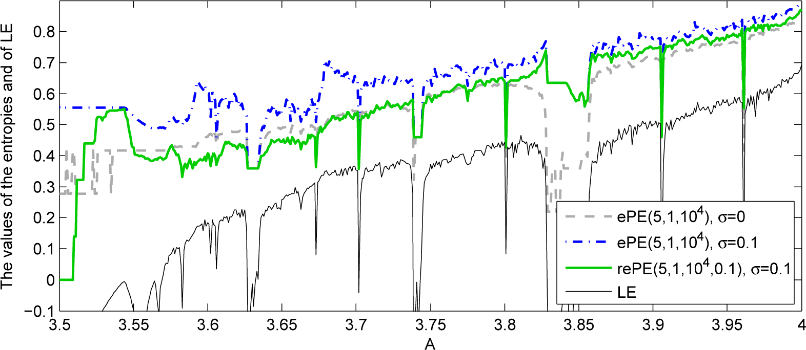
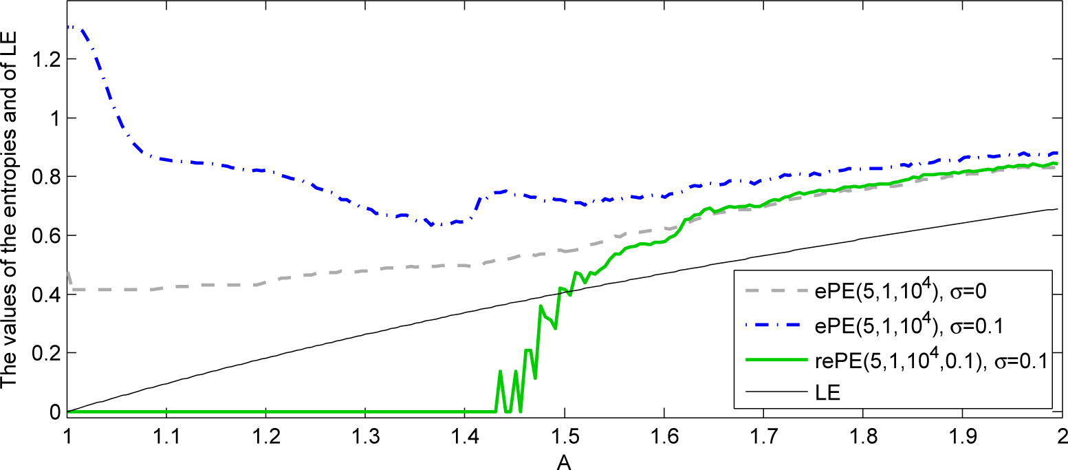
Example 2. For illustration, we consider ePE and rePE of a time series generated by the logistic map t_lm(x) = Ax(1 − x) and by the tent map t_Tm(x) = A min(x, 1 − x) for the random starting point x and for the parameter A ∈ [3.5,4] and A ∈ (1,2], respectively. We add to the time series a centered Gaussian white noise with standard deviation 0.1. In Figures 3 and 4 one can see that when noise is added, the values of rePE for η = 0.1 are more reliable than the values of ePE Indeed, the values of rePE of a noisy time series are closer to the values of ePE of a time series without noise than the values of ePE of a noisy time series. For comparison, the values of Lyapunov exponent are also presented in the plots (see Remark 1).

In Figure 4 the values of rePE for the parameter A < 1.5 are equal to 0, this is related to the small number of 0.1-robust ordinal patterns, whereas the values of ePE of noisy time series provide the wrong impression that the complexity of original time series for the parameter A < 1.5 is large.

Let us summarize that the introduced rePE provides better robustness with respect to observational noise than the ePE. However, the rePE has two drawbacks. Firstly, one needs to set the parameter η in order to compute rePE, which is ambiguous. Secondly, rePE has a slower computational algorithm than ePE (see [37] for details).

2.4. Examples and Comparisons

In this subsection we compare the following practically important properties of ApEn, SampEn, ePE and eCE: the efficiency of computing the entropies (Example 3), the ability to assess a large complexity of a time series (Example 4), and the ability to discriminate between different complexities of EEG data (Example 5).

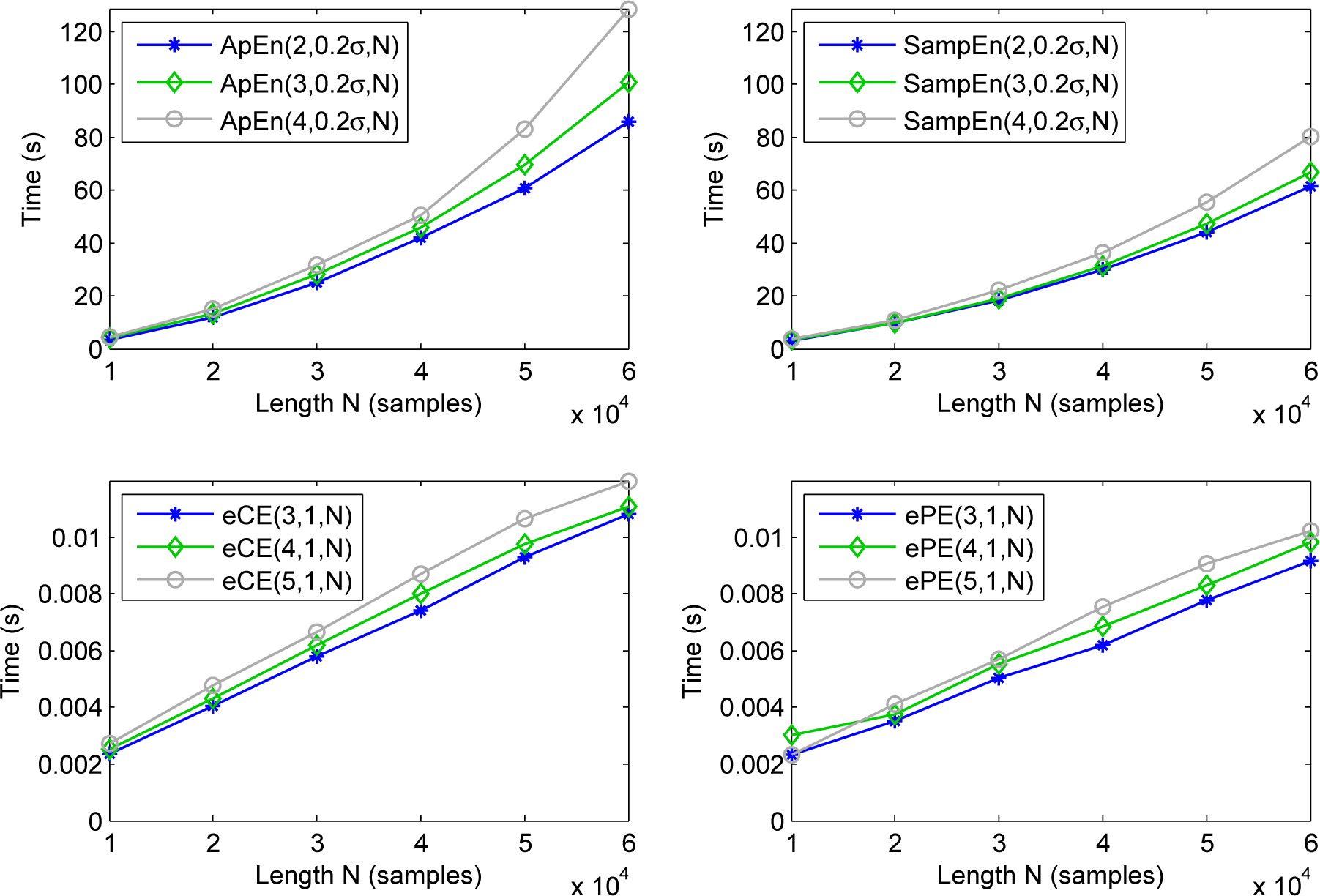
Example 3. In this example we illustrate that ePE and eCE have more efficient algorithms for computing than ApEn and SampEn (see [50–52] for the MATLAB scripts and [37,53,54] for the original papers introducing the corresponding fast algorithms), which allows for processing large datasets in real time. (Note that the algorithms introduced in [51,52] are the fastest for computing of ApEn and SampEn, to our knowledge.)

We present the efficiency of the methods in terms of computational time and storage use with dependence on the length N of a considered time series in

Table 1. Efficiency of computing the entropies.

Quantity	Method of computing	Computational time	Storage use
ApEn	[54]	$O(N^{\frac{3}{2}})$	O(N)
SampEn	[54]	$O(N^{\frac{3}{2}})$	O(N)
ePE	[53]	O(N)	O((d + 1)!(d + 1))
eCE	[37] based on [53]	O(N)	O((d + 1)!(d + 1))

(we refer to [37,53,54] for justification).

For better illustration we present in Figure 5 the computational times of the entropies with dependence on the length N of a time series generated by the logistic map T_LM(x) = 4(1 − x)x. The experiments were performed in MATLAB version R2013b and the times were measured by the standard function “cputime” in OS Linux 2.6.37.6-24, processor Intel(R) Core(TM) i5-2400 CPU @ 3.10Hz. The time was averaged over several trials. One can see that the values of ePE and eCE are computed about 10⁴ times faster for the same lengths of time series.

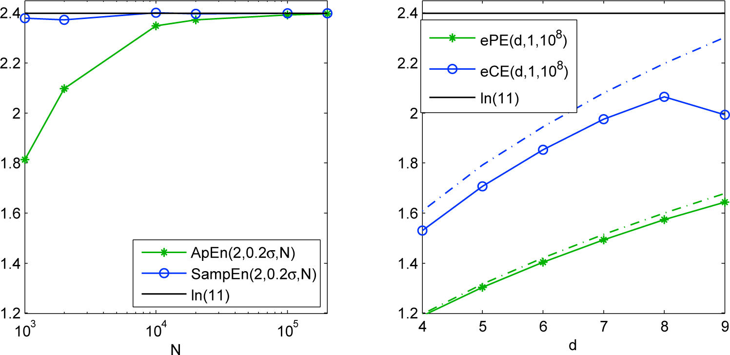
Example 4. In this example we illustrate the ability of the entropies to assess large complexity of a time series. For that we consider a time series generated by the β-transformation for β = 11, i.e., T₁₁(x) = 11x mod 1, with the Kolmogorov–Sinai entropy ln(11) [46] (see also Remark 1). In Figure 6 one can see that the values of ApEn and SampEn approach ln(11) starting from the length N ≈ 10⁵ of a time series, whereas the values of ePE and eCE are bounded by (5) and (8) (green and blue dashed line, correspondingly), which is not enough for d ≤ 9. (Note that d > 9 is usually not used in applications since it requires rather large length of a time series N > 5 · 10! points for the reliable estimation of complexity [41].) The value of eCE for d = 9 is underestimated due to the insufficient length N = 10⁸, see for details [55].

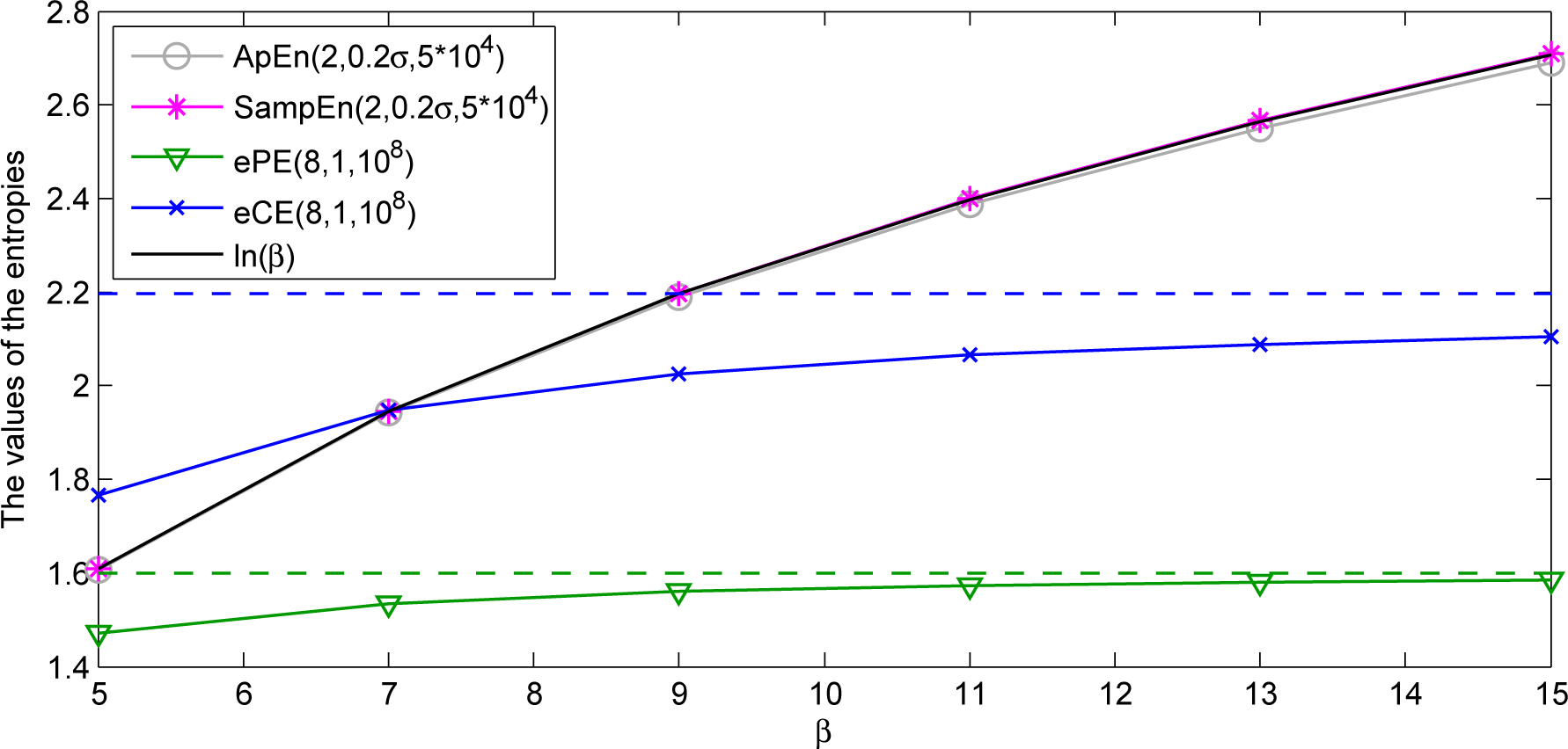
The consequence of the upper bounds of the entropies is that ePE and eCE fail to distinguish between the complexities larger than$\frac{ln((d+1)!)}{d}$ and ln(d + 1), correspondingly. For example, one can see in Figure 7 that the values of ePE and eCE are almost the same for the values β = 5, 7,…,15 of the beta-transformation T_β(x) = βx mod 1 with the Kolmogorov-Sinai entropy lnβ [46] (see Remark 1), whereas the values of ApEn and SampEn estimate the complexity correctly.

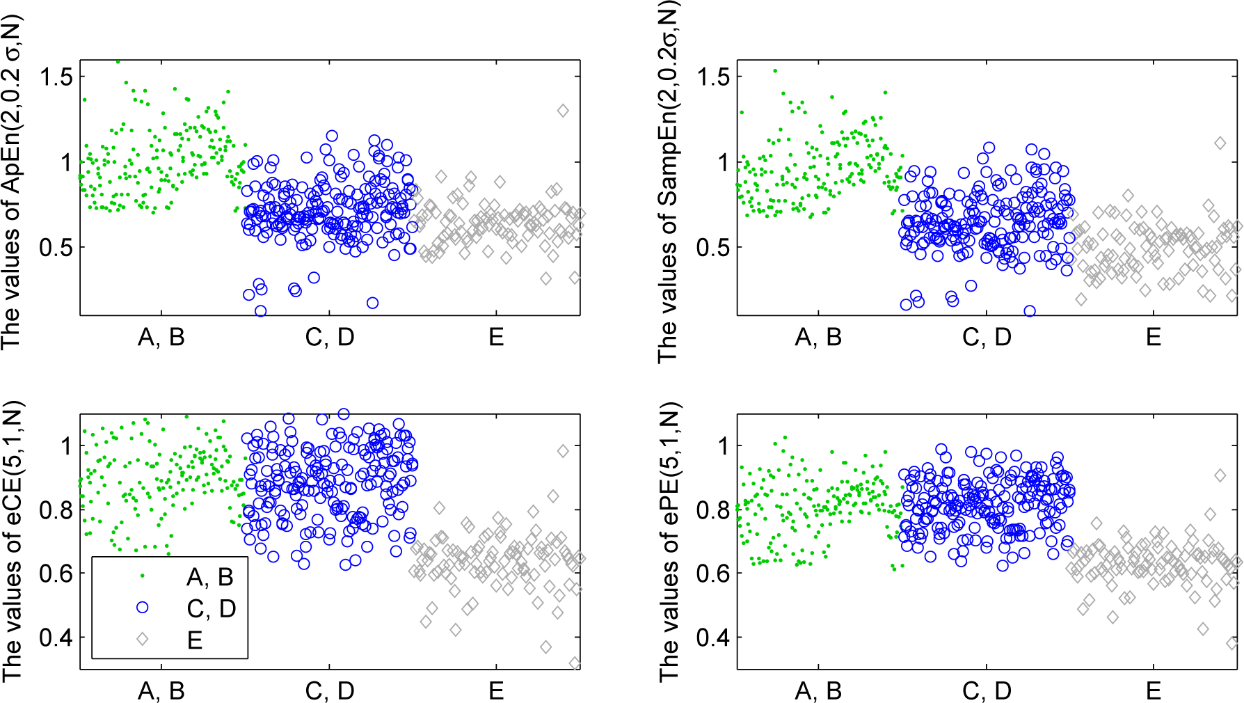
Example 5. In this example we illustrate the ability of ApEn, SampEn, ePE and eCE to discriminate between different complexities of EEG recordings from the Bonn EEG Database (available online at [56]). There are five groups of datasets [57]:

• (A) surface EEG recorded from healthy subjects with open eyes,
• (B) surface EEG recorded from healthy subjects with closed eyes,
• (C) intracranial EEG recorded from subjects with epilepsy during a seizure-free period from hippocampal formation of the opposite hemisphere of the brain,
• (D) intracranial EEG recorded from subjects with epilepsy during a seizure-free period from within the epileptogenic zone,
• (E) intracranial EEG recorded from subjects with epilepsy during a seizure period.

Each group contains 100 one-channel EEG recordings of 23.6 s duration recorded at a sampling rate of 173.61 Hz, and the recordings are free from artifacts; we refer to [57] for more details. For simplicity, we further refer to the recordings from the group A as “recordings A”, the recordings from the group B as “recordings B”, etc.

In Figure 8 one can see that ApEn and SampEn separate the recordings A and B from the recordings C, D and E, whereas ePE and eCE separate the recordings E from the recordings A, B, C and D.

Therefore it is a natural idea to present the values of ePE and eCE versus the values of ApEn and SampEn for each recording. Indeed, in Figure 9 one can see a good separation between the recordings A and B, the recordings C and D, and the recordings E.

We have found also that varying the delay τ can be used for separation between the groups of recordings when computing ePE and eCE. For example, in Figure 10 one can see that the delay τ = 1 provides a separation of the recordings A and B from other recordings, whereas the delay τ = 3 provides a separation of the recordings E from other recordings. The natural idea now is to present the values of ePE and eCE versus themselves for different delays τ. In Figure 11 one can see a good separation between the recordings A and B, the recordings C and D, and the recordings E.

The results of discrimination are presented only for illustration of discrimination ability of ePE, eCE, ApEn and SampEn, therefore we do not compare the results with other methods (for a review of classification methods applied for the Bonn EEG Database see [58]).

Application of the entropies to the epileptic data from Bonn EEG Database has shown the following:

• It can be useful to apply approximate entropy, sample entropy, empirical permutation entropy and empirical conditional entropy of ordinal patterns together since they reveal different features of the dynamics underlying a time series.
• It can be useful to apply empirical permutation entropy and empirical conditional entropy of ordinal patterns for different delays τ since they reveal different features of the dynamics underlying a time series.

3. Ordinal-Patterns-Based Segmentation of EEG and Clustering of EEG Segments

Complexity measures (including those considered in the previous section) are usually only interpretable for stationary time series [1,32,60] and may be unreliable when stationarity fails. (Roughly speaking, a time series is stationary if parameters of this time series do not change over time. See Section 3.1 in [59] for a rigorous definition and details.) Meanwhile, most of real-world time series are non-stationary [59]. A time point where some characteristic of a time series changes is called a change-point. The detection of change-points is a typical problem of time series analysis [59,61–64]; in particular it provides a segmentation of time series into stationary segments. In this section we suggest an ordinal-patterns-based method for change-point detection. Note that methods for change-point detection are usually introduced for stochastic processes; then time series are considered as particular realizations of stochastic processes and ordinal patterns are a special kind of statistic over these realizations. In this paper we only explain the idea of ordinal-patterns-based change-point detection and present our approach in an “intuitive” way. Therefore we omit some theoretical discussions that will appear in [55] and define all the concepts immediately for time series, which may be useful for applications. According to the results of our experiments, the here suggested ordinal-patterns-based method provides much better detection of change-points than the first ordinal-patterns-based method introduced in [30,31]. The performance of our method is comparable but a bit worse than performance of the classical method described in [65]; however, our method requires less a priori information about the time series. The theoretical justification and comparison with other methods for change-point detection will appear in forthcoming publications and, in particular, in [55].

We describe the general idea of ordinal-patterns-based change-point detection (Section 3.1) and introduce a statistic for detecting change-points in time series (Section 3.2). In this paper we use segmentation for revealing the segments of time series corresponding to certain states of the underlying system. For this we combine ordinal-patterns-based segmentation with classification of the obtained segments by means of clustering (grouping of objects in such a way that objects from the same group are in certain sense more similar than objects from different groups) of time series. We sketch the idea of ordinal-patterns-based clustering in Section 3.3. Finally, we apply ordinal-patterns-based segmentation and clustering to EEG time series in Section 3.4.

3.1. The Idea of Ordinal-Patterns-Based Change-Point Detection

The approach described below can be generalized to an arbitrary τ ∈ N, but to simplify the notation, in this section we fix the delay τ = 1. For further discussion we need the following definition.

Definition 7. A real-valued time series${(x_i)}_{i=0}^N$ has the sequence${(\pi )}_{i=d}^N$ of ordinal patterns of order d if the vector (x_i−d, x_i−d+1,…, x_i) has the ordinal pattern π_i for i = d, d + 1,…, N.

The idea of the ordinal-patterns-based change-point detection is to search for change-points in the sequence of ordinal patterns of a time series instead of searching for change-points in the time series itself. For doing this, we should assume further that all change-points in the time series are structural in the sense of the following definition.

Definition 8. Let${(x_i)}_{i=0}^N$ be a time series with a single change-point t^∗ ∈ {0, 1,…, N} (i.e., ${(x_i)}_{i=0}^N$ is non-stationary and t^∗ splits it into two stationary segments). We say that t^∗ is a structural change-point if the sequence${({\pi }_i)}_{i=d}^N$ of ordinal patterns of order d is also non-stationary.

The assumption that change-points in a time series are structural seems to be realistic in many cases. An indicator of a structural change-point is provided by frequencies of ordinal patterns. Given t ∈ {d + 1, d + 2,…, N − d}, denote distributions of relative frequencies of ordinal patterns of order d before and after the moment t by p¹(t) and p²(t) respectively, where ${\mathbf{p}}^k(t)={({\mathit{p}}_j^k(t))}_{j=0}^{(d+1)!-1}$ for k = 1, 2. If there is a structural change-point at t = t^∗, then it holds p¹(t^∗), p²(t^∗); on the contrary, for a stationary time series it holds

$${\mathbf{p}}^1(t)\approx {\mathbf{p}}^2(t)$$

(11)

for all t ∈ {T_min, T_min + 1,…, N − T_min}, where T_min = 5(d + 1)! is the length of a time series required for a reliable estimation of the relative frequencies of ordinal patterns according to (6).

The first method of ordinal-patterns-based change-point detection introduced in [30,31] is, roughly speaking, based on using (11). Here we suggest another approach described in the following subsection.

3.2. Change-Point Detection Using the CEofOP Statistic

We begin with introducing a statistic based on the empirical conditional entropy of ordinal patterns (Definition 4) that allows to estimate a structural change-point in a time series. Let us denote here the empirical conditional entropy of ordinal patterns of a time series ${(x_i)}_{i=0}^N$ for order d ∈ ℕ and delay τ = 1 by eCE $(d,{(x_i)}_{i=0}^N)$.

Definition 9. The CEofOP (“Conditional-Entropy-of-Ordinal-Patterns-based”) statistic of a time series${(x_i)}_{i=0}^N$ at time point t ∈ {d, d + 1, …, N − 1} for order d ∈ ℕ is given by

$$\text{CEofOP}(t;d)=(N-2d)\text{eCE}(d,{(x_i)}_{i=0}^N)-(t-d)\text{eCE}(d,{(x_i)}_{i=0}^t)-(N-t-d)\text{eCE}(d,{(x_i)}_{i=t}^N).$$

(12)

Remark 3. We can also rewrite CEofOP in an explicit form using (7):

$$\begin{array}{c}\text{CEofOP}(t;d)=-(N-2d){\displaystyle \sum _{j=0}^{(d+1)!-1}{\displaystyle \sum _{l=0}^{(d+1)!-1}{p}_j^0(t)q_{j,l}^0(t)\ln q_{j,l}^0(t)}}\\ +(t-d){\displaystyle \sum _{j=0}^{(d+1)!-1}{\displaystyle \sum _{l=0}^{(d+1)!-1}{p}_j^1(t)q_{j,l}^1(t)\ln q_{j,l}^1(t)}}\\ +(N-t-d){\displaystyle \sum _{j=0}^{(d+1)!-1}{\displaystyle \sum _{l=0}^{(d+1)!-1}{p}_j^2(t)q_{j,l}^2(t)\ln q_{j,l}^2(t)},}\end{array}$$

(13)

(with 0 ln 0 := 0), where$p_j^k(t)=\frac{\#\{i\in I^k|{\pi }_i=j\}}{\#\{i\in I^k\}}$, $q_{j,l}^k(t)=\frac{\#\{i\in I^k|{\pi }_i=j,{\pi }_{i+1}=l\}}{\#\{i\in I^k|{\pi }_i=j\}}$ for k = 0, 1, 2, and I⁰(t) = {d, d + 1, …, N − 1}, I¹(t) = {d, d + 1, …, t}, I²(t) = {t + d, t + d + 1, …, N − 1}.

The calculation of the CEofOP statistic by (12) requires a reliable estimation of eCE. For this according to (9), the length of a time series should be no smaller than T_min = (d + 1)!(d + 1). Therefore we recommend to consider CEofOP(t; d) only for

$$N>2T_{min}=2(d+1)!(d+1)$$

(14)

and for t ∈ {T_min, T_min + 1,…, N − T_min}, d ∈ ℕ.

If a structural change occurs at some point t^∗, then CEofOP (t; d) tends to attain its maximum at t = t^∗. This happens because the conditional entropy is concave (not only for ordinal patterns but in general, see Section 2.1.3 in [66]), i.e., for all t = T_min, T_min + 1,…, N − T_min it holds

$$\text{eCE}(d,{(x_i)}_{i=0}^N)\ge \frac{t-d}{N-2d}\text{eCE}(d,{(x_i)}_{i=0}^t)+\frac{N-t-d}{N-2d}\text{eCE}(d,{(x_i)}_{i=t}^N).$$

(15)

Thus the CEofOP statistic provides the following estimate of a single change-point t^∗:

$$\widehat{t*}=\underset{t=T_{min,}{T}_{min}+1,\dots ,N-T_{min}}{\arg max}\text{CEofOP}(t;d).$$

(16)

Remark 4. Note that if a time series${(x_i)}_{i=0}^N$ is stationary, then for N being sufficiently large, (15) holds with equality for all t = T_min, T_min + 1, …, N − T_min (see [55] for the proof). This fact is important for detecting change-points.

In the following example we illustrate the estimation of a change-point by the CEofOP statistic.

Example 6. Consider a time series${(x_i)}_{i=0}^N$ given by

$$x_i=\{\begin{array}{ll}\sin \frac{\pi }{2}i,\hfill & i<\gamma N\hfill \\ \sin \frac{\pi }{2}(2i+1),\hfill & i\ge \gamma N\hfill \end{array}$$

(17)

for N ∈ ℕ, i = 0, 1,…, N, and γ ∈ (0, 1) such that γN ∈ ℕ. This time series has a structural change-point t^∗ = γN; a part of the time series containing the change-point is shown in Figure 12.

Consider the corresponding sequence${({\pi }_i)}_{i=d}^N$ of ordinal patterns of order d = 1 (recall that there are two ordinal patterns of order d = 1, “increasing” and “decreasing”, see Definition 2). The sequence${({\pi }_i)}_{i=d}^N$ is a realization of a piecewise stationary Markov chain, the probabilities of ordinal patterns are equal to$\frac{1}{2}$both before and after the change, while the transition probabilities (i.e., probabilities qj_,l that the ordinal pattern l succeeds the ordinal pattern j) are given by the matrices

$$\left(\begin{array}{cc}\frac{1}{2}& \frac{1}{2}\\ \frac{1}{2}& \frac{1}{2}\end{array}\right)\mathit{\text{and}}\left(\begin{array}{cc}0& 1\\ 1& 0\end{array}\right)$$

Let t = θN ∈ ℕ for θ ∈ (0, 1), then from the general representation (13) of CEofOP it follows that

$$\text{CEofOP}(\theta N;1)=\{\begin{array}{ll}\frac{\gamma }{2}\ln \frac{2-\gamma }{\gamma }-\ln (2-\gamma )+\frac{2-\theta -\gamma }{2}\ln \frac{2-\theta -\gamma }{1-\theta }+\frac{\gamma -\theta }{2}\ln \frac{\gamma -\theta }{1-\theta }N,\hfill & \theta <\gamma \hfill \\ \frac{\gamma }{2}\ln \frac{2-\gamma }{\theta }-\ln (2-\gamma )+\frac{2\theta -\gamma }{2}\ln \frac{2\theta -\gamma }{1-\theta }+(1-\theta )\ln 2)N,\hfill & \theta \ge \gamma \hfill \end{array}.$$

An easy computation shows that CEofOP(θN; 1) has a unique maximum at θ = γ, which provides a detection of the change-point. In particular, for$\gamma =\frac{1}{2}$ we obtain:

$$\text{CEofOP}(\theta N;1)=\{\begin{array}{ll}\left(\ln 2-\frac{3}{4}\ln 3+\frac{3-2\theta }{4}\ln \frac{3-2\theta }{2-2\theta }+\frac{1-2\theta }{4}\ln \frac{1-2\theta }{2-2\theta }\right)N,\hfill & \theta <\frac{1}{2}\hfill \\ \left((2-2\theta )\ln 2-\frac{3}{4}\ln 3-\theta \ln \theta +\frac{4\theta -1}{4}\ln (4\theta -1)\right)N,\hfill & \theta \ge \frac{1}{2}\hfill \end{array}.$$

Figure 13 shows that CEofOP(θN; 1) attains a distinct maximum at$\theta =\frac{1}{2}$ (shown by the vertical line).

Now we describe how the CEofOP statistic solves two classical problems of change-point detection [61]:

Problem 1. (at most one change): Given at most one change-point t^∗ ∈ ℕ, one needs to find an estimate $\widehat{t*}\in \mathbb{N}$ or conclude that no change has occurred.

Problem 2. (multiple change-points): Given N_st ∈ ℕ stationary segments bounded by the change-points $t_1^{*},t_2^{*},\dots ,t_{N_{st}-1}^{*}\in \mathrm{\mathbb{N}}$, one calculates an estimate ${\widehat{N}}_{\text{st}}\in \mathrm{\mathbb{N}}$ of N_st and estimates $\widehat{t_1^{*}},\widehat{t_2^{*}},\dots ,{\widehat{t_{\widehat{N}}^{*}}}_{{}_{\text{st}-1}}\in \mathrm{\mathbb{N}}$ change-points.

To solve Problem 1 we need to verify whether $\widehat{t*}$ is actually a change-point. This is a classical problem of change-point detection (see Section 1.1.2.2 in [59]); to solve it, we compare the value of CEofOP $(\widehat{t*};d)$ with a certain threshold h: if CEofOP $(\widehat{t*};d)\ge h$ then one decides that there is a change-point in $\widehat{t*}$, otherwise it is concluded that no change has occurred. We compute the threshold h using block bootstrapping from the sequence of ordinal patterns (see [63,64] for a comprehensive description of the block bootstrapping; since this approach is rather often used we do not go into details). The solution of Problem 1 using the CEofOP statistic is described in

Algorithm 1. Detecting at most one structural change-point using the CEofOP statistic.

(Appendix A.1).

To detect multiple change-points (Problem 2) we use an algorithm consisting of two main steps:

Step 1: preliminary estimation of change-points using the binary segmentation procedure [67]. The idea of the binary segmentation is simple: the single change-point detection procedure is applied to the original time series; if a change-point is detected, then it splits the time series into two segments. This procedure is repeated iteratively for the obtained segments until all of them either do not contain change-points or are shorter than 2T_min.

Step 2: verification of change-points and rejection of the false ones (the idea of this step as an improvement of the binary segmentation procedure is suggested in [65]).

The details of these two steps are displayed in

Algorithm 2. Detecting multiple structural change-points using the CEofOP statistic.

(Appendix A.2).

3.3. Ordinal-Pattern-Distributions Clustering

In this subsection, we consider classification of segments of time series with respect to the ordinal pattern distributions.

Definition 10. A clustering of time series segments such that every segment is represented by the distribution of relative frequencies of ordinal patterns is called ordinal-pattern-distributions (OPD) clustering.

Given an M-dimensional time series for M ∈ ℕ, a distribution of relative frequencies of ordinal patterns is characterized by a vector $\mathbf{p}={(p_l)}_{l=0}^{M(d+1)!-1}$, where pj_{+(m−1)(d+1)!} represents the relative frequency of the ordinal pattern j in the m-th component of the time series for j = 0, 1, …, (d + 1)! − 1, m = 1, 2,…, M.

In the first papers devoted to OPD clustering [31,68], the authors split time series into short segments of fixed length and then cluster these segments. Instead, we segment time series by means of the change-point detection via the CEofOP statistic and then cluster the obtained segments that are pseudo-stationary in the sense of having no structural change-points. Our approach is motivated by the criticism of segmenting time series without taking into account their structure (see, for instance, Section 7.3.1 in [62]).

To cluster the vectors representing the distributions of ordinal patterns, we use the k-means algorithm [69] with the squared Hellinger distance. The squared Hellinger distance between the distributions of frequencies of ordinal patterns in the i-th and k-th segments of a time series is defined by

$${\rho }_H({\mathbf{p}}^i,{\mathbf{p}}^k)=\frac{1}{2}{\displaystyle \sum _{j=0}^{(d+1)!-1}{\left(\sqrt{p_j^i}-\sqrt{p_j^k}\right)}^2.}$$

Using the squared Hellinger distance for the ordinal-patterns-based clustering was first suggested in [68]; for the justification of this choice we refer to [55].

3.4. An Application of Ordinal-Patterns-Based Segmentation and Ordinal-Pattern-Distributions Clustering to Sleep EEG

In this subsection we employ ordinal-patterns-based segmentation and OPD clustering to sleep stage discrimination, which is a relevant problem in biomedical research [70,71]. To investigate sleep stages, one measures electrical activity of brain by means of EEG. According to the classification in [72], there are six stages of human state during the night:

• the waking state (W);
• two stages of light sleep (S1, S2);
• two stages of deep sleep (S3, S4);
• rapid eye movement (REM) sleep.

Note that according to the modern classification stage S4 is not distinguished from S3 [70].

Construction of a generally recognized automatic procedure for sleep stage discrimination is problematic due to the complex nature of EEG signal; thus discrimination of sleep EEG is mainly carried out manually by experts [70]. They assign a sleep stage (W, REM, S1–S4) to every 30 s epoch of the EEG recording [70]; the result is often visualized by a hypnogram.

Example 7. We consider the dataset described in [73] and provided by [74]. It consists of eight whole-night recordings with manually scored hypnograms (four recordings contain EEG monitored during 24 h, for them we consider only the sleep related parts). Further we refer to the recordings according to their names in the dataset (see

Table 2. Agreement between the manual scoring and the ordinal-patterns-based discrimination of sleep EEG.

Recording	Amount of sleep-related epochs	Correctly identified epochs
sc4002	1050	73.6%
sc4012	1150	73.7%
sc4102	1050	83.8%
sc4112	750	79.2%
st7022	944	61.2%
st7052	1032	81.3%
st7121	1027	80.7%
st7132	852	68.9%
Overall	7855	75.4%

for the list of the names). Each recording contains two EEG time series (recorded from the Fpz-Cz and Pz-Oz locations) sampled at 100 Hz.

The ordinal-patterns-based discrimination of sleep EEG consists of the following steps:

• EEG time series are filtered to the band 1 Hz to 45 Hz (with the Butterworth filter of order 5).
• The ordinal-patterns-based segmentation procedure (described by

  Algorithm 3. Ordinal-patterns-based segmentation of multivariate time series.

  in Appendix A.3) is employed for d = 4, which is the maximal order satisfying 2(d + 1)!(d + 1) < N (see (14)) for N = 3000 corresponding to the epoch length of 30 s.
• OPD clustering (as described in Section 3.3, for d = 4) is applied to the segments of all recordings. The number of clusters 8 is chosen, the transition-state segments (see Algorithm 3) are considered as unclassified. We deliberately choose the number of clusters larger than the number of sleep stages since for different persons EEG may be significantly different (especially in the waking state). Therefore, we analyze the obtained clusters and group them into larger classes:

• class “AWAKE”: three clusters;
• class “LIGHT SLEEP”: three clusters (one of these clusters may be associated with stage S1 and two others with stage S2, but we do not distinguish between S1 and S2 since the amount of the epochs corresponding to S1 is small);
• class “DEEP SLEEP”: one cluster (the manual scoring was done according to the old classification [72], while the modern classification [70] does not distinguish stages S3 and S4);
• class “REM”: one cluster.

Figure 14 illustrates the outcome of the ordinal-patterns-based discrimination of sleep EEG in comparison with the hypnogram.

Table 3. Amount of 30 s epochs from the class specified by the column with the manual score specified by the row (for all eight recordings from the dataset [74]).

		Results of ordinal-patterns-based discrimination
Manual score		AWAKE	LIGHT SLEEP	DEEP SLEEP	REM	unclassified
	W	440	165	0	103	3
	S1, S2	110	3234	227	635	19
	S3, S4	0	404	880	10	5
	REM	0	244	0	1365	0
	Unclassified	3	6	1	1	0

presents the correspondence between the results of ordinal-patterns-based discrimination against manual scoring. Amounts of correctly identified epochs are shown in bold. The share of correctly identified epochs for every recording is shown in Table 2.

As one can see from Table 2 the overall agreement between the manual scoring and the suggested ordinal-patterns-based method for sleep EEG discrimination in Example 7 is 75.4%. This is comparable with the results for the same dataset reported by researchers that use different discrimination methods. In particular, in the studies [75] and [76], the authors obtain agreement with the manual scoring for 74.5% and 81.5% of the epochs, respectively. In contrast to the methods suggested in [75,76], the ordinal-patterns-based discrimination is based on completely data-driven procedures of ordinal-patterns-based segmentation and OPD clustering, and does not use any expert knowledge about the data. This fact emphasizes the potential of ordinal-patterns-based segmentation and OPD clustering and encourages further research in this direction.

4. Summary and Conclusions

We have discussed the applicability and performance of three empirical measures based on the distribution of ordinal patterns in time series. These are the empirical permutation entropy (ePE), the empirical conditional entropy of ordinal patterns (eCE), and the robust empirical permutation entropy (rePE). Whereas the ePE is well established and eCE is recently introduced [15], the rePE is a new concept proposed for dealing with noisy data.

We have pointed out that from the viewpoint of computer resources (computational time and memory requirements) the algorithms for computing ePE and eCE, introduced in [15,37], are better than the algorithms for computing ApEn and SampEn introduced in [54]. This is interesting in the case of considering large time series. We have demonstrated on the examples of the logistic and the tent family that rePE could be a robust alternative to ePE in the case of observational noise. Therefore, a further investigation of rePE seems to be useful. Further, the comparison of the entropies was done on the base of EEG recordings from the Bonn EEG Database (available online at [56]). Here it was discussed how good the considered quantifiers separate data of three groups: group 1 consisting of healthy subjects, group 2 consisting of subjects with epilepsy in a seizure-free period, and group 3 consisting of subjects with epilepsy in a seizure period. We have illustrated that plotting the values of ApEn and SampEn versus the values of ePE and eCE provides a good separation between the three groups, as well as plotting the values of ePE and eCE versus themselves for different delays. We therefore conclude that the combined use of ApEn, SampEn, ePE and eCE or the combined use of ePE and eCE seems to be useful for discrimination purposes.

We have suggested a method for classifying time series on the basis of investigating their ordinal pattern distributions. The method consists of two steps: segmentation of time series into pseudo-stationary segments and clustering of the obtained segments. We have performed the segmentation of time series on the basis of change-point analysis providing the boundaries of segments. As change-points, we have considered time points where the ordinal structure of a time series was changing, as proposed in [30]. In order to identify such points we have introduced the CEofOP (“Conditional-Entropy-of-Ordinal-Patterns-based”) statistic, which is based on eCE. For finding all relevant change-points, we have used the binary segmentation procedure [67] in combination with block bootstrapping [63,64]. After segmenting the time series as described, the obtained segments were clustered on the basis of their ordinal pattern distributions by means of a commonly-used cluster algorithm (k-means clustering with the squared Hellinger distance). The method was applied to the discrimination of sleep EEG data. Here we have obtained good results for considering eight clusters. The obtained clusters could be very well assigned to one of the following four groups: “AWAKE”, “LIGHT SLEEP”, “DEEP SLEEP”, and “REM”. This is somewhat surprising because no information on the structure of data related to special sleep stages was used, but shows some potential of the method in sleep stage discrimination.

We have demonstrated the potential of ePE and eCE for the discrimination of states of a system based on time series analysis, but would also like to emphasize that for these purposes a combined use of different entropy concepts, ordinal and non-ordinal ones, can be useful. For this, a better knowledge of the relationship and of the differences of such concepts would be important and should be addressed in further research.

References

- Bandt, C.; Pompe, B. Permutation entropy—A natural complexity measure for time series. Phys. Rev. E 2002, 88. [Google Scholar] [CrossRef]
- Li, X.; Ouyang, G.; Richards, D.A. Predictability analysis of absence seizures with permutation entropy. Epilepsy Res. 2007, 77, 70–74. [Google Scholar]
- Cao, Y.; Tung, W.W.; Gao, J.B.; Protopopescu, V.A.; Hively, L.M. Detecting dynamical changes in time series using the permutation entropy. Phys. Rev. E 2004, 70. [Google Scholar] [CrossRef]
- Keller, K.; Lauffer, H. Symbolic analysis of high-dimensional time series. Int. J. Bifurc. Chaos 2003, 13, 2657–2668. [Google Scholar]
- Ouyang, G.; Dang, C.; Richards, D.A.; Li, X. Ordinal pattern based similarity analysis for EEG recordings. Clin. Neurophysiol. 2010, 121, 694–703. [Google Scholar]
- Olofsen, E.; Sleigh, J.W.; Dahan, A. Permutation entropy of the electroencephalogram: A measure of anaesthetic drug effect. Br. J. Anaesth. 2008, 101, 810–821. [Google Scholar]
- Li, D.; Li, X.; Liang, Z.; Voss, L.J.; Sleigh, J.W. Multiscale permutation entropy analysis of EEG recordings during sevoflurane anesthesia. J. Neural Eng. 2010, 7. [Google Scholar] [CrossRef]
- Nicolaou, N.; Georgiou, J. The use of permutation entropy to characterize sleep electroencephalograms. Clin. EEG Neurosci. 2011, 42, 24–28. [Google Scholar]
- Graff, B.; Graff, G.; Kaczkowska, A. Entropy Measures of Heart Rate Variability for Short ECG Datasets in Patients with Congestive Heart Failure. Acta Phys. Polonica B Proc. Suppl. 2012, 5, 153–158. [Google Scholar]
- Parlitz, U.; Berg, S.; Luther, S.; Schirdewan, A.; Kurths, J.; Wessel, N. Classifying cardiac biosignals using ordinal pattern statistics and symbolic dynamics. Comput. Biol. Med. 2012, 42, 319–327. [Google Scholar]
- Frank, B.; Pompe, B.; Schneider, U.; Hoyer, D. Permutation entropy improves fetal behavioural state classification based on heart rate analysis from biomagnetic recordings in near term fetuses. Med. Biol. Eng. Comput. 2006, 44, 179–187. [Google Scholar]
- Bian, C.; Qin, C.; Ma, Q.D.Y.; Shen, Q. Modified permutation-entropy analysis of heartbeat dynamics. Phys. Rev. E 2012, 85. [Google Scholar] [CrossRef]
- Amigó, J.M.; Keller, K. Permutation entropy: One concept, two approaches. Eur. Phys. J. Spec. Top. 2013, 222, 263–273. [Google Scholar]
- Amigó, J.M. Permutation Complexity in Dynamical Systems; Springer-Verlag: Berlin and Heidelberg, Germany, 2010. [Google Scholar]
- Unakafov, A.M.; Keller, K. Conditional entropy of ordinal patterns. Physica D 2013, 269, 94–102. [Google Scholar]
- Acharya, U.R.; Joseph, K.P.; Kannathal, N.; Lim, C.M.; Suri, J.S. Heart rate variability: A review. Med. Biol. Eng. Comput. 2006, 44, 1031–1051. [Google Scholar]
- Bruhn, J.; Röpcke, H.; Hoeft, A. Approximate entropy as an electroencephalographic measure of anesthetic drug effect during desflurane anesthesia. Anesthesiology 2000, 92, 715–726. [Google Scholar]
- Bruhn, J.; Röpcke, H.; Rehberg, B.; Bouillon, T.; Hoeft, A. Electroencephalogram approximate entropy correctly classifies the occurrence of burst suppression pattern as increasing anesthetic drug effect. Anesthesiology 2000, 93, 981–985. [Google Scholar]
- Jordan, D.; Stockmanns, G.; Kochs, E.F.; Pilge, S.; Schneider, G. Electroencephalographic order pattern analysis for the separation of consciousness and unconsciousness: An analysis of approximate entropy, Permutation Entropy, recurrence rate, and phase coupling of order recurrence plots. Anesthesiology 2008, 109, 1014–1022. [Google Scholar]
- Acharya, U.R.; Faust, O.; Kannathal, N.; Chua, T.; Laxminarayan, S. Non-linear analysis of EEG signals at various sleep stages. Comput. Methods Programs Biomed. 2005, 80, 37–45. [Google Scholar]
- Burioka, N.; Miyata, M.; Cornélissen, G.; Halberg, F.; Takeshima, T.; Kaplan, D.T.; Suyama, H.; Endo, M.; Maegaki, Y.; Nomura, T.; et al. Approximate entropy in the electroencephalogram during wake and sleep. Clin. EEG Neurosci. 2005, 36, 21–24. [Google Scholar]
- Kannathal, N.; Choo, M.L.; Acharya, U.R.; Sadasivan, P.K. Entropies for detection of epilepsy in EEG. Comput. Methods Programs Biomed. 2005, 80, 187–194. [Google Scholar]
- Ocak, H. Automatic detection of epileptic seizures in EEG using discrete wavelet transform and approximate entropy. Expert Syst. Appl. 2009, 36, 2027–2036. [Google Scholar]
- Richman, J.S.; Moorman, J.R. Physiological time-series analysis using approximate entropy and sample entropy. Am. J. Physiol.-Heart Circ. Physiol. 2000, 278, 2039–2049. [Google Scholar]
- Yentes, J.M.; Hunt, N.; Schmid, K.K.; Kaipust, J.P.; McGrath, D.; Stergiou, N. The Appropriate use of approximate entropy and sample entropy with short data sets. Ann. Biomed. Eng. 2013, 41, 349–365. [Google Scholar]
- Lake, D.E.; Richman, J.S.; Griffin, M.P.; Moorman, J.R. Sample entropy analysis of neonatal heart rate variability. Am. J. Physiol.-Regul. Integr. Comp. Physiol. 2002, 283, R789–R797. [Google Scholar]
- Abásolo, D.; Hornero, R.; Espino, P.; Alvarez, D.; Poza, J. Entropy analysis of the EEG background activity in Alzheimer’s disease patients. Physiol. Meas. 2006, 27. [Google Scholar] [CrossRef]
- Jouny, C.C.; Bergey, G.K. Characterization of early partial seizure onset: Frequency, complexity and entropy. Clin. Neurophysiol. 2012, 123, 658–669. [Google Scholar]
- Chen, W.; Zhuang, J.; Yu, W.; Wang, Z. Measuring complexity using FuzzyEn, ApEn, and SampEn. Med. Eng. Phys. 2009, 31, 61–68. [Google Scholar]
- Sinn, M.; Ghodsi, A.; Keller, K. Detecting change-points in time series by kernel mean matching of ordinal pattern distributions. Proceedings of the 28th Conference on Uncertainty in Artificial Intelligence, Catalina Island, CA, USA, 15–17 August 2012; pp. 786–794.
- Sinn, M.; Keller, K.; Chen, B. Segmentation and classification of time series using ordinal pattern distributions. Eur. Phys. J. Spec. Top. 2013, 222, 587–598. [Google Scholar]
- Pincus, S.M. Approximate entropy as a measure of system complexity. Proc. Natl. Acad. Sci. 1991, 88, 2297–2301. [Google Scholar]
- Grassberger, P.; Procaccia, I. Estimation of the Kolmogorov entropy from a chaotic signal. Phys. Rev. A 1983, 28, 2591–2593. [Google Scholar]
- Eckmann, J.-P.; Ruelle, D. Ergodic theory of chaos and strange attractors. Rev. Mod. Phys. 1985, 57, 617–656. [Google Scholar]
- Walters, P. An Introduction to Ergodic Theory; Springer: New York, NY, USA, 2000. [Google Scholar]
- Broer, H.; Takens, F. Dynamical Systems and Chaos; Springer: New York, NY, USA, 2010. [Google Scholar]
- Unakafova, V.A. Investigating measures of complexity for dynamical systems and for time series. Ph.D. Thesis, draft version, University of Lubeck, Lubeck, Germany, 2015. [Google Scholar]
- Pincus, S.M. Approximate entropy (ApEn) as a complexity measure. Chaos 1995, 5, 110–117. [Google Scholar]
- Keller, K.; Unakafov, A.M.; Unakafova, V.A. On the relation of KS entropy and permutation entropy. Physica D 2012, 241, 1477–1481. [Google Scholar]
- Keller, K.; Emonds, J.; Sinn, M. Time series from the ordinal viewpoint. Stoch. Dyn. 2007, 2, 247–272. [Google Scholar]
- Amigó, J.M.; Zambrano, S.; Sanjuán, M.A.F. Combinatorial detection of determinism in noisy time series. Europhys. Lett. 2008, 83. [Google Scholar] [CrossRef]
- Riedl, M.; Müller, A.; Wessel, N. Practical considerations of permutation entropy. Eur. Phys. J. Spec. Top. 2013, 222, 249–262. [Google Scholar]
- Li, J.; Yan, J.; Liu, X.; Ouyang, G. Using permutation entropy to measure the changes in EEG signals during absence seizures. Entropy 2014, 16, 3049–3061. [Google Scholar]
- The European Epilepsy Database. Available online: http://epilepsy-database.eu/ accessed on 19 September 2014.
- Bandt, C.; Keller, G.; Pompe, B. Entropy of interval maps via permutations. Nonlinearity 2002, 15, 1595–1602. [Google Scholar]
- Choe, H.C. Computational Ergodic Theory; Springer: New York, NY, USA, 2005. [Google Scholar]
- Sprott, J.C. Chaos and Time-Series Analysis; Oxford University Press: Oxford, UK, 2003. [Google Scholar]
- Zanin, M.; Zunino, L.; Rosso, O.A.; Papo, D. Permutation entropy and its main biomedical and econophysics applications: A review. Entropy 2012, 14, 1553–1577. [Google Scholar]
- Morabito, F.C.; Labate, D.; La Foresta, F.; Bramanti, A.; Morabito, G.; Palamara, I. Multivariate multi-scale permutation entropy for complexity analysis of Alzheimer’s disease EEG. Entropy 2012, 14, 1186–1202. [Google Scholar]
- Unakafova, V.A. Fast Permutation Entropy. MATLAB Central File Exchange. Available online: http://www.mathworks.com/matlabcentral/fileexchange/44161-fast-permutation-entropy accessed on 12 August 2014.
- Lee, K. Fast Approximate Entropy. MATLAB Central File Exchange. Available online: http://www.mathworks.com/matlabcentral/fileexchange/32427-fast-approximate-entropy/content/ApEn.m accessed on 12 August 2014.
- Lee, K. Fast Sample Entropy. MATLAB Central File Exchange. Available online: http://www.mathworks.com/matlabcentral/fileexchange/35784-sample-entropy accessed on 12 August 2014.
- Unakafova, V.A.; Keller, K. Efficiently measuring complexity on the basis of real-world data. Entropy 2013, 15, 4392–4415. [Google Scholar]
- Pan, Y.-H.; Wang, Y.-H.; Liang, S.-F.; Lee, K.-T. Fast computation of sample entropy and approximate entropy in biomedicine. Comput. Methods Programs Biomed. 2011, 104, 382–396. [Google Scholar]
- Unakafov, A.M. Ordinal-patterns-based segmentation and discrimination of time series with applications to EEG data. Ph.D. Thesis, draft version, University of Lubeck, Lubeck, Germany, 2015. [Google Scholar]
- Bonn EEG Database. Available online: http://epileptologie-bonn.de accessed on 12 August 2014.
- Andrzejak, R.G.; Lehnertz, K.; Mormann, F.; Rieke, C.; David, P.; Egler, C.E. Indications of nonlinear deterministic and finite-dimensional structures in time series of brain electrical activity: Dependence on recording region and brain state. Phys. Rev. E 2001, 64. [Google Scholar] [CrossRef]
- Tzallas, A.T.; Tsipouras, M.G.; Fotiadis, D.I. Epileptic seizure detection in EEGs using time–frequency analysis. IEEE Trans. Inf. Technol. Biomed. 2009, 13, 703–710. [Google Scholar]
- Basseville, M.; Nikiforov, I.V. Detection of Abrupt Changes: Theory and Application; Prentice-Hall, Inc.: Upper Saddle River, NJ, USA, 1993. [Google Scholar]
- Richman, J.S.; Lake, D.E.; Moorman, J.R. Sample Entropy. Methods Enzymol. 2004, 384, 172–184. [Google Scholar]
- Carlstein, E.; Muller, H.G.; Siegmund, D. Change-Point Problems; Institute of Mathematical Statistics: Hayward, CA, USA, 1994. [Google Scholar]
- Brodsky, B.E.; Darkhovsky, B.S. Non-Parametric Statistical Diagnosis. Problems and Methods; Kluwer Academic Publishers: Dordrecht, The Netherlands, 2000. [Google Scholar]
- Polansky, A.M. Detecting change-points in Markov chains. Comput. Stat. Data Anal. 2007, 51, 6013–6026. [Google Scholar]
- Kim, A.Y.; Marzban, C.; Percival, D.B.; Stuetzle, W. Using labeled data to evaluate change detectors in a multivariate streaming environment. Signal Process. 2009, 89, 2529–2536. [Google Scholar]
- Brodsky, B.E.; Darkhovsky, B.S.; Kaplan, A.Y.; Shishkin, S.L. A nonparametric method for the segmentation of the EEG. Comput. Methods Programs Biomed. 1999, 60, 93–106. [Google Scholar]
- Han, T.S.; Kobayashi, K. Mathematics of Information and Coding. Transl. from the Japanese by J. Suzuki.; American Mathematical Society: Providence, RI, USA, 2002. [Google Scholar]
- Vostrikova, L.Y. Detecting disorder in multidimensional random processes. Sov. Math. Dokl. 1981, 24, 55–59. [Google Scholar]
- Brandmaier, A.M. Permutation Distribution Clustering and Structural Equation Model Trees. Ph.D. Thesis, University of Saarland, Saarbrucken, Germany, 2012. [Google Scholar]
- Abonyi, J.; Feil, B. Cluster Analysis for Data Mining and System Identification; Springer: Berlin, Germany, 2007. [Google Scholar]
- Silber, M.H.; Ancoli-Israel, S.; Bonnet, M.H.; Chokroverty, S.; Grigg-Damberger, M.M.; Hirshkowitz, M.; Kapen, S.; Keenan, S.A.; Kryger, M.H.; Penzel, T.; et al. The visual scoring of sleep in adults. J. Clin. Sleep Med. 2007, 3, 121–131. [Google Scholar]
- Libenson, M.H. Practical Approach to Electroencephalography; Elsevier Health Sciences: Philadelphia, PA, USA, 2012. [Google Scholar]
- Rechtschaffen, A.; Kales, A. A Manual of Standardized Terminology, Techniques and Scoring System for Sleep Stages of Human Subjects; Public Health Service US Government Printing Office: Washington, DC, USA, 1968. [Google Scholar]
- Kemp, B.; Zwinderman, A.H.; Tuk, B.; Kamphuisen, H.A.C.; Oberyé, J.J.L. Analysis of a sleep-dependent neuronal feedback loop: The slow-wave microcontinuity of the EEG. IEEE-BME 2000, 47, 1185–1194. [Google Scholar]
- Goldberger, A.L.; Amaral, L.A.N.; Glass, L.; Hausdorff, J.M.; Ivanov, P.C.; Mark, R.G.; Mietus, J.E.; Moody, G.B.; Peng, C.-K.; Stanley, H.E. PhysioBank, PhysioToolkit, and PhysioNet: Components of a new research resource for complex physiologic signals. Circulation 2000, 101, e215–e220. [Google Scholar]
- Berthomier, C.; Drouot, X.; Herman-Stoïca, M.; Berthomier, P.; Prado, J.; Bokar-Thire, D.; Benoit, O.; Mattout, J.; d’Ortho, M.-P. Automatic analysis of single-channel sleep EEG: Validation in healthy individuals. Sleep 2007, 30, 1587–1595. [Google Scholar]
- Ronzhina, M.; Janoušek, O.; Kolářová, J.; Nováková, M.; Honzík, P.; Provazník, I. Sleep scoring using artificial neural networks. Sleep Med. Rev. 2012, 16, 251–263. [Google Scholar]
Figure 1.
The ordinal patterns of order d = 2.
Figure 2.
Empirical permutation entropy of EEG data with epileptic seizure.
Figure 3.
Empirical permutation entropy and 0.1-robust empirical permutation entropy of a time series generated by the logistic map; σ stands for the standard deviation of added centered Gaussian white noise.
Figure 4.
Empirical permutation entropy and 0.1-robust empirical permutation entropy of a time series generated by the tent map; σ stands for the standard deviation of added centered Gaussian white noise.
Figure 5.
Comparison of the computational times, measured by the MATLAB function “cputime”, of the approximate entropy, sample entropy, empirical permutation entropy and empirical conditional entropy of ordinal patterns computed with the MATLAB scripts from [51,52], [50] (“PE.m”) and [37] (“CE.m”), correspondingly.
Figure 6.
Approximate entropy, sample entropy, empirical permutation entropy and empirical conditional entropy of ordinal patterns of a time series generated by the β-transformation for β = 11 with dependence on the length N and order d.
Figure 7.
The values of approximate entropy, sample entropy, empirical permutation entropy and empirical conditional entropy of ordinal patterns of a time series generated by the beta-transformation with dependence on the parameter β.
Figure 8.
The values of the entropies of the recordings from the groups A and B, C and D, and E; N = 4097.
Figure 9.
The values of empirical permutation entropy and empirical conditional entropy of ordinal patterns versus the values of approximate entropy and sample entropy; N = 4097.
Figure 10.
Empirical permutation entropy and empirical conditional entropy of ordinal patterns of the recordings A and B, C and D, and E, N = 4097.
Figure 11.
The values of ePE(5, 1, N) versus the values of ePE(5, 3, N) and the values of eCE(5, 1, N) versus the values of eCE(5, 3, N), N = 4097.
Figure 12.
Part of the time series given by (17) with the change-point marked by the red vertical line.
Figure 13.
The CEofOP statistic for the time series given by (17).
Figure 14.
Hypnogram (bold curve) and the results of ordinal-patterns-based discrimination of sleep EEG (white color corresponds to class AWAKE, light gray to LIGHT SLEEP, gray to DEEP SLEEP, dark gray to REM, red to unclassified segments) for recording st7121 from the dataset [74].