Sliding-Mode Synchronization Control for Uncertain Fractional-Order Chaotic Systems with Time Delay

Abstract

Specifically setting a time delay fractional financial system as the study object, this paper proposes a single controller method to eliminate the impact of model uncertainty and external disturbances on the system. The proposed method is based on the stability theory of Lyapunov sliding-mode adaptive control and fractional-order linear systems. The controller can fit the system state within the sliding-mode surface so as to realize synchronization of fractional-order chaotic systems. Analysis results demonstrate that the proposed single integral, sliding-mode control method can control the time delay fractional power system to realize chaotic synchronization, with strong robustness to external disturbance. The controller is simple in structure. The proposed method was also validated by numerical simulation.

1. Introduction

Recent years have seen a great deal of research on chaos control, in which many studies have focused specifically on fractional-order chaotic systems. Fractional differential equations not only provide a novel mathematical tool, but further, more successful mathematical models of systems [1,2]. As research regarding chaotic systems has continually intensified, an increasing number of control and synchronization methods specific to chaotic systems have been proposed, verified, and applied effectively [3]. An integer order chaotic system is the result of idealized processing of an actual chaotic system. Fractional-order chaotic systems show enhanced universal application and practicability, however [4]. Generally, stability analysis of integer-order chaotic system controllers adopts Lyapunov stability theory; for stability analysis of a fractional-order system, fractional-order system stability theory is more common, or a combination of both theories [5].

Some synchronous control methods have already been proposed for fractional-order chaotic systems [6], including the drive response method, sliding-mode control method, Lyapunov equation method, self-adaption control method, active control method, nonlinear feedback control method, and generalized synchronization method [7–12]. The sliding-mode adaptive robust control, for one, is not only characterized by quick responsiveness, excellent dynamic characteristics, robustness, and insensitiveness to external changes, but is able to control uncertainty in the system, among other attractive advantages. One notable recent study [13] adopted a sliding-mode control to realize the synchronization of a three dimensional fractional-order chaotic system. The control system, however, was quite simple and did not account for unknown parameters which may occur during real world application, nor external disturbances to the system or impact of time delay on system synchronization. Recently, Zhang et al. [14] developed a single-state adaptive-feedback controller containing a novel fractional integral sliding surface to synchronize a class of fractional-order chaotic systems based on sliding mode variable structure control theory and adaptive control technique. Tian et al. [15] applied the sliding mode control strategy to stabilize a class of fractional-order chaotic systems with input nonlinearity. Toopchi et al. [16] proposed an adaptive integral sliding mode control scheme for synchronization of hyper chaotic Zhou systems. Another study [17] adopted a method to build corresponding response system according to the driving system, performing adaptive estimation of uncertain items considering the effects of uncertain factors to design a nonlinear adaptive controller. The controller did not require knowledge of the upper boundary of uncertainties, was simple in structure, and showed strong robustness to uncertainties including system disturbances; however, the method is not applicable to synchronization of fractional-order chaotic systems, and its response system is dependent on the drive system structure.

The purpose of this study is the design of a synchronization method of sliding-mode adaptive robust control, with a single controller, applicable to external disturbances and uncertainties in fractional-order chaotic systems with time delay. The proposed method utilizes the sliding-mode adaptive synchronization method of integer-order chaotic systems, specifically according to relevant disadvantages shown in previous research [15–17]. The effectiveness of the method was verified by numerical simulation results and in contrast to some results from reference [18].

2. Results and Discussion

2.1. Definitions and Lemma

The most frequently used definitions for the general fractional calculus are Riemann-Liouville definition, Caputo definition and Grunwald-Letnikov definition [15,19,20].

Definition 1. The αth order Riemann-Liouville fractional integration is given by:

$${}_{t_0}{I}_t^{a}f(t)=\frac{1}{\mathrm{\Gamma }(a)}{\displaystyle {\int }_{t_0}^t\frac{f(\tau )}{{(t-\tau )}^{1-a}}d\tau }$$

(1)

where Γ(·) is the Gamma function.

Definition 2. For n – 1 < α ≤ n, n ∈ R, the Riemann-Liouville fractional derivative definition of order α is defined as:

$${}_{t_0}{D}_t^{a}f(t)=\frac{d^{a}f(t)}{d{t}^a}=\frac{1}{\mathrm{\Gamma }(n-a)}\frac{d^n}{d{t}^n}{\displaystyle {\int }_{t_0}^t\frac{f(\tau )}{{(t-\tau )}^{a-n+1}}d\tau =\frac{d^n}{d{t}^n}{I}^{n-a}f(t)}$$

(2)

Definition 3. The Grunwald-Letnikov fractional derivative definition of order α is written as:

$${}_{t_0}{D}_t^{a}f(t)=\underset{h\to 0}{\lim }\frac{1}{h^a}{\displaystyle \sum _{j=0}^{\infty }{(-1)}^j\left(\begin{array}{l}a\\ j\end{array}\right)f(t-jh)}$$

(3)

Lemma 1. (Barbalat’s Lemma [21]) If ε: R → R is a uniformly continuous function for t ≥ 0, and if the limit of the integral$\underset{t\to \infty }{\lim }{\displaystyle {\int }_0^t\epsilon (\tau )}d\tau$ exist and is finite, then$\underset{t\to \infty }{\lim }\epsilon (t)=0$.

2.2. Numerical Method for Solving Fractional Differential Equations

The PC (Predictor, Corrector) method which was proposed by Diethelm et al. [22] is generally used to solve fractional differential equations (FDE). Let us consider the following differential equations:

$${}_{t_0}D{}_t^{a}y(t)=r(y(t),t),0\le t\le T$$

(4)

and:

$$y^{(k)}(0)=y_0^{(k)},k=0,1,2,\cdots ,m-1$$

(5)

where:

$${}_{t_0}{D}_t^{a}y(t)=\{\begin{array}{ll}\frac{1}{\mathrm{\Gamma }(m-a)}{\displaystyle {\int }_0^t\frac{f^{(m)}(\tau )}{{(t-\tau )}^{a-m+1}}d\tau }& m-1<a<m\\ \frac{d^{a}y(t)}{d{t}^a}& a=m\end{array}$$

(6)

and m is the first integer larger than the a. The solution of the Equation (4) is equivalent to the Volterra integral equation:

$$y(t)={\displaystyle \sum _{k=0}^{[a]-1}{y}_0^{(k)}\frac{t^k}{k!}}+\frac{1}{\mathrm{\Gamma }(a)}{\displaystyle {\int }_0^t{(t-\lambda )}^{a-1}r(y(\lambda ),\lambda )d\lambda }$$

(7)

let:

$$h=T/N,t_n=nh,n=0,1,2\cdots ,N$$

(8)

Then Equation (8) can be discretized as follows:

$$y_h(t_{n+1})={\displaystyle \sum _{k=0}^{[a]-1}{y}_0^{(k)}\frac{t_{n+1}^k}{k!}}+\frac{h^a}{\mathrm{\Gamma }(a+2)}r(y_h^p(t_{n+1}),t_{n+1})+\frac{h^a}{\mathrm{\Gamma }(a+2)}{\displaystyle \sum _{j=0}^n{p}_{j,n+1}r(y_h(t_j),t_j)}$$

(9)

where predicted value $y_h^p(t_{n+1})$ is determined by:

$$y_h^p(t_{n+1})={\displaystyle \sum _{k=0}^{[a]-1}{y}_0^{(k)}\frac{t_{n+1}^k}{k!}}+\frac{h^a}{\mathrm{\Gamma }(a)}{\displaystyle \sum _{j=0}^n{q}_{j,n+1}r(y_h(t_j),t_j)}$$

(10)

and:

$$p_{j,n+1}=\{\begin{array}{ll}{n}^{a+1}-(n-a){(n+1)}^a& j=0\\ {(n+2-j)}^{a+1}+{(n-j)}^{a+1}-2{(n-j+1)}^{a+1}& 1\le j\le n\\ 1& j=n+1\end{array}$$

(11)

Hence, for approximating the Equation (6), the predictor formula is given by:

$$q_{j,n+1}=\frac{h^a}{a}({(n+1-j)}^a-{(n-j)}^a),n>0$$

(12)

In this method, the error is:

$$e=\underset{j=0,1,\mathrm{2...},N}{\max }|X(t_j)-X_h(t_j)|=O\left(h^{\min \{2,1+a\}}\right)$$

(13)

Thus, we can obtain the numerical solution of a fractional order system by using the above mentioned algorithm.

2.3. Sliding Surface and Single Controller

Here, we select the 3D fractional financial system expressed as follows:

$$\begin{array}{l}{D}_t^{q_1}{x}_1=x_3+\left[x_2\left(t-\tau \right)-a\right]x_1\\ D_t^{q_2}{x}_2=1-b{x}_2-{\left[x_1\left(t-\tau \right)\right]}^2\\ D_t^{q_3}{x}_3=-x_1\left(t-\tau \right)-c{x}_3\end{array}$$

(14)

where $D_t^q=d^q/d{t}^q$ is the Caputo differential operator, 0 < q < 1, and x = (x₁, x₂, x₃)^T is the state vector of the system.

System (14) is the driving system. The response system without control is:

$$\begin{array}{l}{D}_t^{q_1}{y}_1=y_3+\left[y_2\left(t-\tau \right)-a\right]y_1\\ D_t^{q_2}{y}_2=1-b{y}_2-{\left[y_1\left(t-\tau \right)\right]}^2\\ D_t^{q_3}{y}_3=-y_1\left(t-\tau \right)-c{y}_3\end{array}$$

(15)

The error system can be derived from System (14) and System (15):

$$\begin{array}{l}{D}_t^{q_1}{e}_1=e_3+y_1{y}_2\left(t-\tau \right)-x_1{x}_2\left(t-\tau \right)-a{e}_1\\ D_t^{q_2}{e}_2=-b{e}_2-\left[x_1\left(t-\tau \right)+y_1\left(t-\tau \right)\right]e_1\left(t-\tau \right)\\ D_t^{q_3}{e}_3=-e_1\left(t-\tau \right)-c{e}_3\end{array}$$

(16)

The formula above can be modified as follows:

$$\begin{array}{l}{D}_t^{q_1}{e}_1=g_1\left(e_1,e_2,e_3\right)\\ D_t^{q_2}{e}_2=g_2\left(e_1,e_2,e_3\right)\\ D_t^{q_3}{e}_3=g_3\left(e_1,e_2,e_3\right)\end{array}$$

(17)

Uncertain items of the error system ∆ f(y, t) are integration of model perturbation, external disturbance, and non-modeled sections. An unknown but always existing constant ρ is defined; all ρ must satisfy the following equation:

$$\Vert \mathrm{\Delta }\Vert \le \rho <\infty$$

(18)

where U is a synchronous controller. By designing a reasonable single controller u(t) ∈ Rⁿ, the error system becomes stable, gradually, so as to realize the synchronization between the driving system and response system. The following must be satisfied:

$$\underset{t\to \infty }{\lim }\Vert e\left(t\right)\Vert =\underset{t\to \infty }{\lim }\Vert y\left(t\right)-x\left(t\right)\Vert =0$$

(19)

The error system can be modified as:

$$\begin{array}{l}{D}_t^{q_1}{e}_1=g_1\left(e_1,e_2,e_3\right)+\mathrm{\Delta }f\left(y,t\right)+U\\ D_t^{q_2}{e}_2=g_2\left(e_1,e_2,e_3\right)\\ D_t^{q_3}{e}_3=g_3\left(e_1,e_2,e_3\right)\end{array}$$

(20)

As a conjecture, if Formulas (14) and (16) are smooth and continuous within the neighborhood region of e₁ = 0, the following subsystem is defined:

$$\begin{array}{l}{D}_t^{q_2}{e}_2=g_2\left(0,e_2,e_3\right)\\ D_t^{q_3}{e}_3=g_3\left(0,e_2,e_3\right)\end{array}$$

(21)

For all e₂, e_3, e₂ = 0, e₃ = 0, is consistent exponential stability.

The following controller forms are considered:

$$u\left(t\right)=u_{eq}\left(t\right)+u_d\left(t\right)$$

(22)

where u_eq(t) is equivalent control system, and u_d(t) is the system’s approach rate.

To ensure the system stays at the equilibrium point, (system synchronization,) sliding-mode surface s was designed as follows:

$$s=D_t^{q-1}{e}_1+{\displaystyle {\int }_0^{t}a{e}_1\left(\tau \right)d\tau }$$

(23)

If the sliding manifold meets s = 0 and $\dot{s}=0$, equivalent control u_eq(t) can be obtained:

$$u_{eq}\left(t\right)=s\dot{s}=-e_3+e_2\left(t-\tau \right)$$

(24)

In order to realize the path curve of the system as it reaches a given sliding manifold, the approach rate u_d(t) must satisfy:

$$u_d\left(t\right)=k\mathrm{sgn}\left(s\right)k<0$$

(25)

Theorem 1. Consider the sliding-mode dynamics (20), the system is asymptotically stable.

Proof: According to the continuous frequency distributed model of fractional integrator [23–25], the fractional-order sliding-mode dynamics (20) is exactly equivalent to the following infinite dimensional ordinary differential equations:

$$\begin{array}{l}\frac{\partial z_1(\omega ,t)}{\partial t}=-\omega z_1(\omega ,t)+D_t^{q_1}{e}_1\\ e_1={\displaystyle {\int }_0^{\infty }{\mu }_1(\omega )}{z}_1(\omega ,t)d\omega \\ \frac{\partial z_2(\omega ,t)}{\partial t}=-\omega z_2(\omega ,t)+D_t^{q_2}{e}_2\\ e_2={\displaystyle {\int }_0^{\infty }{\mu }_2(\omega )}{z}_2(\omega ,t)d\omega \\ \frac{\partial z_3(\omega ,t)}{\partial t}=-\omega z_3(\omega ,t)+D_t^{q_3}{e}_3\\ e_3={\displaystyle {\int }_0^{\infty }{\mu }_3(\omega )}{z}_3(\omega ,t)d\omega \end{array}$$

(26)

where μ_i(ω) = ((sin(q_iπ))/π) ω^−q_i > 0, i = 1, 2, 3. In above model, z₁(ω,t), z₂(ω,t), z₃(ω,t) are the true state variables, while x(t), y(t), z(t) are the pseudo state variables [26,27]. Then, Lyapunov’s stability theory in [28] can be applied to prove the asymptotic stability of the above system. Selecting a positive definite Lyapunov function:

$$V_1(t)=\frac{1}{2}{\displaystyle \sum _{i=1}^3{\displaystyle {\int }_0^{\infty }{\mu }_i(\omega )z_i^2(\omega ,t)d\omega }}$$

(27)

Taking the derivative of V₁(t) with respect to time, it yields:

$$\begin{array}{l}{\dot{V}}_1(t)=\frac{1}{2}{\displaystyle \sum _{i=1}^3{\displaystyle {\int }_0^{\infty }{\mu }_i(\omega )\frac{\partial z_i^2(\omega ,t)}{\partial t}d\omega }}={\displaystyle \sum _{i=1}^3{\displaystyle {\int }_0^{\infty }{\mu }_i(\omega )z_i(\omega ,t)\frac{\partial z_i(\omega ,t)}{\partial t}d\omega }}\\ ={\displaystyle {\int }_0^{\infty }{\mu }_1(\omega )z_1(\omega ,t)\left[-\omega z_1(\omega ,t)+D_t^{q_1}{e}_1\right]d\omega }\\ +{\displaystyle {\int }_0^{\infty }{\mu }_2(\omega )z_2(\omega ,t)\left[-\omega z_2(\omega ,t)+D_t^{q_2}{e}_2\right]d\omega }\\ +{\displaystyle {\int }_0^{\infty }{\mu }_3(\omega )z_3(\omega ,t)\left[-\omega z_3(\omega ,t)+D_t^{q_3}{e}_3\right]d\omega }\\ =-{\displaystyle \sum _{i=1}^3{\displaystyle {\int }_0^{\infty }\omega {\mu }_i(\omega )z_i^2(\omega ,t)d\omega }}+e_1{D}_t^{q_1}{e}_1+e_2{D}_t^{q_2}{e}_2+e_3{D}_t^{q_3}{e}_3\end{array}$$

(28)

It has been proven that in case of idling mode motion in the system, the sliding-mode surface s meets the following conditions:

$$\begin{array}{c}s=D_t^{q_1-1}{e}_1+{\displaystyle {\int }_0^{t}a{e}_1\left(\tau \right)d\tau }=0\\ \dot{s}=D_t^{q_1}{e}_1+a{e}_1=0\end{array}$$

(29)

The following can be derived:

$$D_t^{q_1}{e}_1=-a{e}_1$$

(30)

If e₁ = 0, then the 2D sub-system $D_t^{q_2}{e}_2=-b{e}_2$, $D_t^{q_3}{e}_3=-c{e}_3$, Then, we have:

$$\begin{array}{l}{\dot{V}}_1(t)=-{\displaystyle \sum _{i=1}^3{\displaystyle {\int }_0^{\infty }\omega {\mu }_i(\omega )z_i^2(\omega ,t)d\omega }}+e_1{D}_t^{q_1}{e}_1+e_2{D}_t^{q_2}{e}_2+e_3{D}_t^{q_3}{e}_3\\ =-{\displaystyle \sum _{i=1}^3{\displaystyle {\int }_0^{\infty }\omega {\mu }_i(\omega )z_i^2(\omega ,t)d\omega }}-a{e}_1^2-b{e}_2^2-c{e}_3^2\end{array}$$

(31)

Since μ_i(ω) > 0, a are non-negative constants, so according to the analysis results of reference [28], we have ${\dot{V}}_1(t)<0$, which implies that the fractional-order sliding-mode dynamics (20) is asymptotically stable. Therefore, the proof is completed. □

Theorem 2. For a controlled error system starting from an arbitrary value, when t → ∞, the trajectory converges to zero ($\underset{t\to \infty }{\lim }{e}_i=0\left(i=1,2,3\right)$). Under the effects of the sliding-mode adaptive controller, the fractional-order driven system and response will realize a gradual synchronization.

It has been proven that in case of sliding mode motion in the system, the sliding-mode surface s meets the following conditions:

$$\begin{array}{l}s=D_t^{q_1-1}{e}_1+{\displaystyle {\int }_0^{t}a{e}_1\left(\tau \right)d\tau }=0\\ \dot{s}=D_t^{q_1}{e}_1+a{e}_1=0\end{array}$$

(32)

The following can be derived:

$$D_t^{q_1}{e}_1=-a{e}_1$$

(33)

Obviously, a > 0. Error e gradually becomes stable. As discussed above, $\underset{t\to \infty }{\lim }{e}_2=0,\underset{t\to \infty }{\lim }{e}_3=0$:

$$\underset{t\to \infty }{\lim }{e}_i=0(i=1,2,3)$$

(34)

The following proves that the error system satisfies the sliding condition s = 0 starting from arbitrary initial conditions. The Lyapunov function is $V=s^2/2$.

The following can be derived:

$$\begin{array}{l}\dot{V}=s\dot{s}=\left(D_t^{q_1}{e}_1+a{e}_1\right)s\\ =\left(e_3+e_2\left(t-\tau \right)-a{e}_1+\mathrm{\Delta }+u\left(t\right)+a{e}_1\right)s\\ =\left(e_3+e_2\left(t-\tau \right)+\mathrm{\Delta }-e_3+e_2\left(t-\tau \right)+k\mathrm{sgn}\left(s\right)\right)s\\ =\left(\mathrm{\Delta }+k\mathrm{sgn}\left(s\right)\right)s\\ \le \left(\rho +k\mathrm{sgn}\left(s\right)\right)|s|\\ \le 0,k\le -\rho \end{array}$$

As long as a proper k value is set and the error system is in line with Lyapunov stability theory after disturbance, the synchronization control method is effective. The error system is also shown here to meet sliding-mode conditions starting from arbitrary initial conditions. Because Formula (34) was established on the sliding-mode surface, the error system can remain at the equilibrium point. In other words, synchronization was maintained between the driving system and controlled response system.

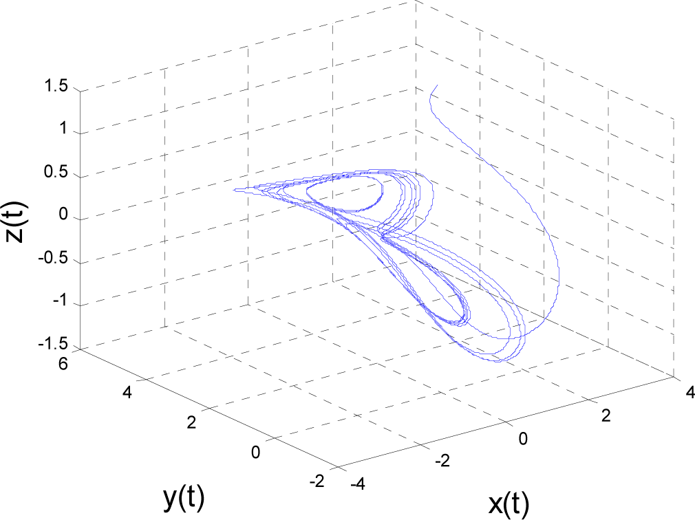
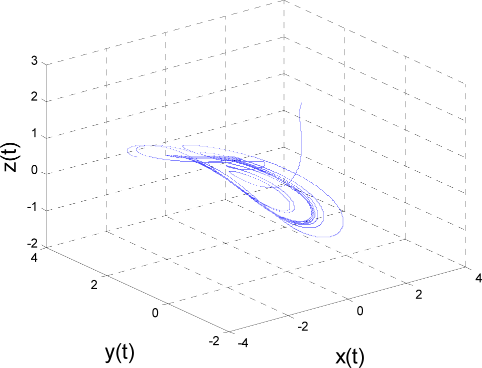
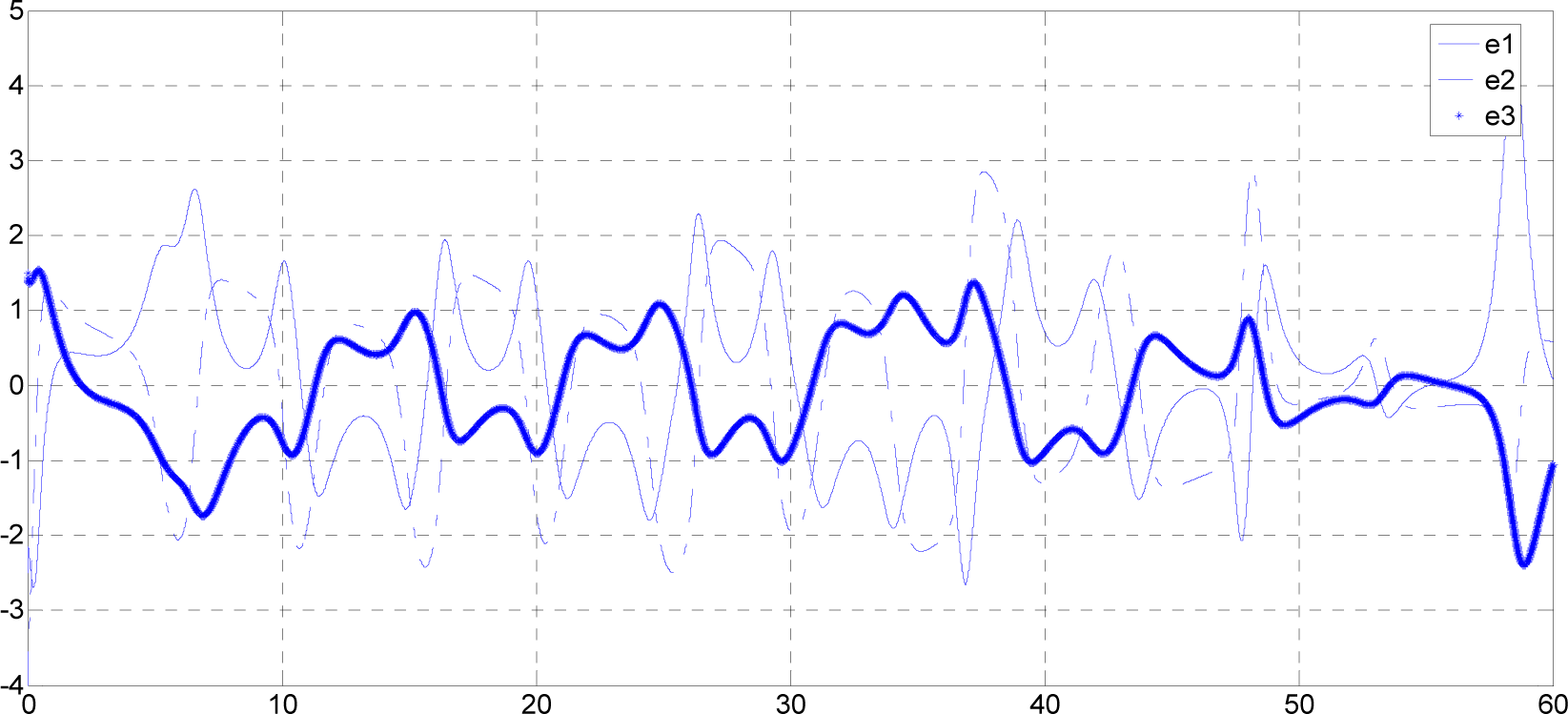
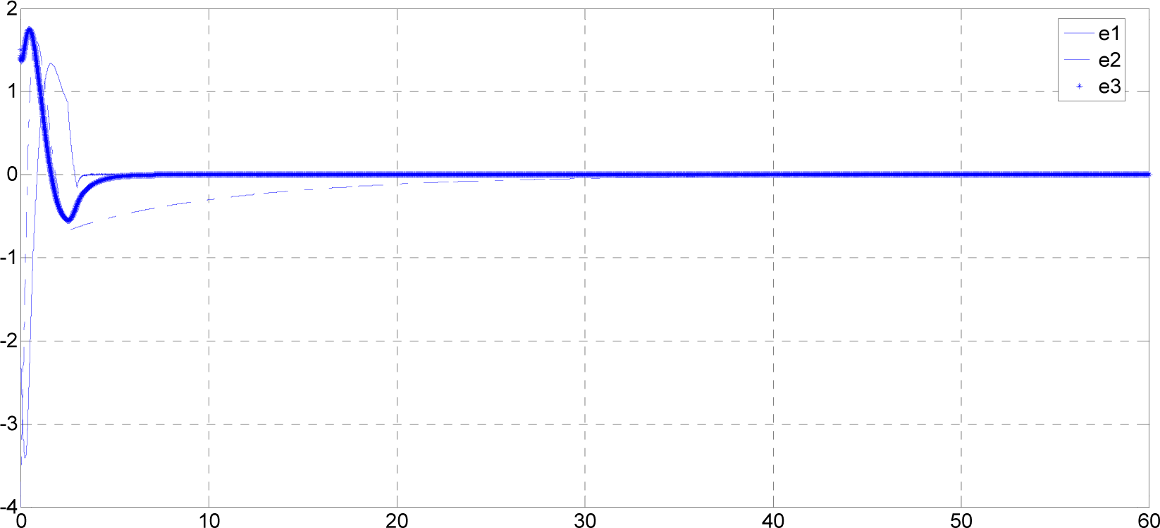
3. Experimental Section

In order to fully legitimize the proposed theory, we performed numerical validation of fractional order-chaos in a financial system.

The driving system is:

$$\begin{array}{l}{D}_t^{0.88}{x}_1=x_3+\left[x_2\left(t-0.06\right)-1\right]x_1\\ D_t^{0.98}{x}_2=1-0.1x_2-{\left[x_1\left(t-0.06\right)\right]}^2\\ D_t^{0.96}{x}_3=-x_1\left(t-0.06\right)-1.2x_3\end{array}$$

(35)

The response system is:

$$\begin{array}{l}{D}_t^{0.88}{y}_1=y_3+\left[y_2\left(t-0.06\right)-1\right]y_1+\mathrm{\Delta }f\left(y,t\right)+U\\ D_t^{0.98}{y}_2=1-0.1y_2-{\left[y_1\left(t-0.06\right)\right]}^2\\ D_t^{0.96}{y}_3=-y_1\left(t-0.06\right)-1.2y_3\end{array}$$

(36)

where the model uncertainty, external disturbance and sector nonlinear input are given by:

$$\mathrm{\Delta }f\left(y,t\right)=0.1\sin (2\pi y_1)$$

(37)

The error system is:

$$\begin{array}{l}{D}_t^{0.88}{e}_1=e_3+y_1{y}_2\left(t-0.06\right)-x_1{x}_2\left(t-0.06\right)-e_1+\mathrm{\Delta }f\left(y,t\right)+U\\ D_t^{0.98}{e}_2=-0.1e_2-\left[x_1\left(t-0.06\right)+y_1\left(t-0.06\right)\right]e_1\left(t-0.06\right)\\ D_t^{0.96}{e}_3=-e_1\left(t-0.06\right)-1.2e_3\end{array}$$

(38)

If e₁ = 0, then the 2d subsystem $D_t^{0.98}{e}_2=-0.1e_2$, $D_t^{0.96}{e}_3=-1.2e_3$, thus $\underset{t\to \infty }{\lim }{e}_2=0,\underset{t\to \infty }{\lim }{e}_3=0$. According to the theorem specified above, under the effect of the single controller, the driving system will maintain synchronization with the response system. Numerical simulation was executed by combining the fractional frequency approximation method and s function in MATLAB. The control law is selected as:

$$u=-e_3+e_2\left(t-\tau \right)-\mathrm{sgn}\left(s\right)$$

(39)

According to the initialization method in [29,30], the initial conditions for fractional differential equations with order between 0 and 1 are constant function of time, so the initial conditions for systems (35) and (36) can be chosen randomly as:

$$\begin{array}{l}{x}_1(t)=x_1(0^{+})=3\\ y_1(t)=y_1(0^{+})=4\\ z_1(t)=z_1(0^{+})=1\\ x_2(t)=x_2(0^{+})=0.5\\ y_2(t)=y_2(0^{+})=0\\ z_2(t)=z_2(0^{+})=2.5\end{array}$$

(40)

With the above fractional orders and initial conditions, systems (35) and (36) possesses a chaotic behavior, as shown in Figures 1 and 2. To observe the control effect of controller, the state trajectories of Equation (38) without control are firstly given in Figure 3. When the controller is activated, we can obtain the desired time responses of system (38), shown in Figure 4. It is not difficult to see that all state trajectories converge to zero asymptotically, which implies that a class of uncertain fractional-order chaotic systems (38) with sector nonlinear input can be stabilized. Reference [18] has the same synchronization time as this paper, but in this paper there is less codes by contrast. Figures 1 and 2 show chaotic attractor images of the driving system and response system, respectively.

4. Conclusions

Based on Lyapunov stability theory and sliding-mode adaptive control method, using a time-delay fractional financial system as an example, this paper proposed a sliding-mode adaptive synchronous control method. The proposed method replaces the common linear sliding-mode control with an integral sliding-mode control. The synchronous control method is applicable to the single controller as-designed, and is altogether applicable to synchronization control of fractional-order chaotic systems.

The proposed method focuses on practicability. Its single controller implies low cost, as well. It is robust against noise, reduces buffeting generated during the control process, and demonstrates favorable control capability for time delay systems. The proposed method is an example of integer-order adaptive synchronization of chaotic systems successfully translated to fractional-order chaotic systems, with certain theoretical and practical significance. Numerical simulation results verified the proposed method’s effectiveness, robustness, and successful control of the study system. Furthermore, the method is easily implemented in engineering applications.

References

1. Wang, D.F.; Zhang, J.Y.; Wang, X.Y. Robust Modified Projective Synchronization of Fractional-Order Chaotic Systems with Parameters Perturbation and External Disturbance. Chin. Phys. B 2013, 22, 100504–100510. [Google Scholar]
2. Yuan, L.G.; Yang, Q.G. Parameter Identification and Synchronization of Fractional-Order Chaotic Systems. Commun. Nonlinear Sci 2012, 17, 305–316. [Google Scholar]
3. Kinzel, W.; Englert, A.; Kanter, I. On Chaos Synchronization and Secure Communication. Philos. Trans. R. Soc. A 2010, 368, 379–389. [Google Scholar]
4. Cui, Z.H.; Cai, X.J.; Zcug, J.C. A New Stochastic Algorithm to Direct Orbits of Chaotic Systems. Int. J. Comput. Appl. Tech 2012, 43, 366–371. [Google Scholar]
5. Chen, L.P.; Qu, J.F.; Chai, Y.; Wu, R.C.; Qi, G.Y. Synchronization of a Class of Fractional-Order Chaotic Neural Networks. Entropy 2013, 15, 3265–3276. [Google Scholar]
6. Zhou, P.; Bai, R.J. The Adaptive Synchronization of Fractional-Order Chaotic System with Fractional-Order (1<q<2) via Linear Parameter Update Law. Nonlinear Dyn 2015, 80, 753–765. [Google Scholar]
7. Mahmoud, G.M.; Mahmoud, E.E. Lag Synchronization of Hyperchaotic Complex Nonlinear Systems. Nonlinear Dyn 2012, 67, 1613–1622. [Google Scholar]
8. Yang, C.C. Synchronization of Rotating Pendulum via Self-learning Terminal Sliding-mode Control Subject to Input Nonlinearity. Nonlinear Dyn 2013, 72, 695–705. [Google Scholar]
9. Abooee, A.; Haeri, M. Stabilisation of Commensurate Fractional-Order Polytopic Non-linear Differential Inclusion Subject to Input Non-linearity and Unknown Disturbances. IET Control Theory Appl 2013, 7, 1624–1633. [Google Scholar]
10. Agrawal, S.K.; Das, S. Projective Synchronization between Different Fractional-Order Hyperchaotic Systems with Uncertain Parameters Using Proposed Modified Adaptive Projective Synchronization Technique. Math. Meth. Appl. Sci 2014, 37, 1232–1239. [Google Scholar]
11. Ma, J.; Qin, H.X.; Song, X.L.; Chu, R.T. Pattern Selection in Neuronal Network Driven by Electric Autapses with Diversity in Time Delays. Int. J. Mod. Phys. B 2015, 29, 1450239. [Google Scholar]
12. Ma, W.; Li, C.; Wu, Y.; Wu, Y. Adaptive Synchronization of Fractional Neural Networks with Unknown Parameters and Time Delays. Entropy 2014, 16, 6286–6299. [Google Scholar]
13. Cao, H.F.; Zhang, R.X. Adaptive Synchronization of Fractional-Order Chaotic System via Sliding-Mode Control. Acta Phys. Sin 2011, 60, 050510. [Google Scholar]
14. Zhang, R.X.; Yang, S. Adaptive Synchronization of Fractional-Order Chaotic Systems via a Single Driving Variable. Nonlinear Dyn 2012, 66, 831–837. [Google Scholar]
15. Tian, X.; Fei, S. Robust Control of a Class of Uncertain Fractional-Order Chaotic Systems with Input Nonlinearity via an Adaptive Sliding Mode Technique. Entropy 2014, 16, 729–746. [Google Scholar]
16. Toopchi, Y.; Wang, J. Chaos Control and Synchronization of a Hyperchaotic Zhou System by Integral Sliding Mode control. Entropy 2014, 16, 6539–6552. [Google Scholar]
17. Deng, W.; Fang, J.; Wu, Z.J. Adaptive Modified Function Projective Synchronization of a Class of Chaotic Systems with Uncerntainties. Acta Phys. Sin 2012, 61, 14050. [Google Scholar]
18. Xin, B.G.; Chen, T. Projective Synchronization of N-Dimensional Chaotic Fractional-Order Systems via Linear State Error Feedback Control. Discrete Dyn. Nat. Soc 2012, 2012, 191063. [Google Scholar]
19. Sabatier, J.; Merveillaut, M.; Malti, R.; Oustaloup, A. On a Representation of Fractional Order Systems: Interests for the Initial Condition Problem, Proceeding 3rd IFAC Workshop on Fractional Differentiation and its Applications, Ankara, Turkey, 5–7 November 2008; p. 1.
20. Sabatier, J.; Merveillaut, M.; Malti, R.; Oustaloup, A. How to Impose Physically Coherent Initial Conditions to a Fractional System. Comm. Nonlinear Sci. Numer. Simulat 2010, 15, 1318–1326. [Google Scholar]
21. Khalil, H.K. Nonlinear Systems; Prentice Hall: Upper Saddle River, NJ, USA, 2002. [Google Scholar]
22. Diethelm, K.; Ford, N. A Predictor-Corrector Approach for the Numerical Solution of Fractional Differential Equations. Nonlinear Dyn 2002, 29, 3–22. [Google Scholar]
23. Trigeassou, J.C.; Maamri, N.; Sabatier, J.; Oustaloup, A. State Variables and Transients of Fractional Order Differential Systems. Comput. Math. Appl 2012, 64, 3117–3140. [Google Scholar]
24. Trigeassou, J.C.; Maamri, N.; Sabatier, J.; Oustaloup, A. Transients of Fractional-Order Integrator and Andderivatives Signal. Image Video Process 2012, 6, 359–372. [Google Scholar]
25. Trigeassou, J.C.; Maamri, N. Initial Conditions and Initialization of Linear Fractional Differential Equations. Signal Process 2011, 91, 427–436. [Google Scholar]
26. Sabatier, J.; Farges, C.; Oustaloup, A. On Fractional Systems State Space Description. J. Vib. Contr 2014, 20, 1076–1084. [Google Scholar]
27. Sabatier, J.; Farges, C.; Merveillaut, M.; Fenetau, L. On observability and Pseudo State Estimation of Fractional Order Systems. Eur. J. Control 2012, 18, 260–271. [Google Scholar]
28. Trigeassou, J.C.; Maamri, N.; Sabatier, J.; Oustaloup, A. A Lyapunov Approach to the Stability of Fractional Differential Equations. Signal Process 2011, 91, 437–445. [Google Scholar]
29. Sabatier, J.; Farges, C. Long Memory Models: A First Solution to the Infinite Energy Storage Ability of Linear Time Invariant Fractional Models, Proceedings of 19th World Congress of the International Federation of Automatic Control, Cape Town, South Africa, 24–29 August 2014; pp. 24–29.
30. Sabatier, J.; Agrawal, O.P.; Tenreiro Machado, J.A. (Eds.) Advances in Fractional Calculus: Theoretical Developments and Applications in Physics and Engineering; Springer: Heidelberg, Germany, 2007.
Figure 1. Fractional-order chaotic attractors of drive system with time delay.
Entropy 17 04202f1
Figure 2. Fractional-order chaotic attractors of response system with time delay.
Entropy 17 04202f2
Figure 3. Error system of chaos system without controller.
Entropy 17 04202f3
Figure 4. Error system of chaos system with controller.
Entropy 17 04202f4
Figure 5. Control effort in suppression while the control law (39) is used.
Entropy 17 04202f5