Article

New Hyperbolic Function Solutions for Some Nonlinear Partial Differential Equation Arising in Mathematical Physics

by
Haci Mehmet Baskonus
1,* and
Hasan Bulut
2
1
Department of Computer Engineering, Tunceli University, Tunceli, 62100, Turkey
2
Department of Mathematics, University of Firat, Elazig, 23119, Turkey
*
Author to whom correspondence should be addressed.
Entropy 2015, 17(6), 4255-4270; https://doi.org/10.3390/e17064255
Submission received: 20 May 2015 / Revised: 15 June 2015 / Accepted: 17 June 2015 / Published: 19 June 2015
(This article belongs to the Section Complexity)

Abstract

:
In this study, we investigate some new analytical solutions to the (1 + 1)-dimensional nonlinear Dispersive Modified Benjamin–Bona–Mahony equation and the (2 + 1)-dimensional cubic Klein–Gordon equation by using the generalized Kudryashov method. After we submitted the general properties of the generalized Kudryashov method in Section 2, we applied this method to these problems to obtain some new analytical solutions, such as rational function solutions, exponential function solutions and hyperbolic function solutions in Section 3. Afterwards, we draw two- and three-dimensional surfaces of analytical solutions by using Wolfram Mathematica 9.

1. Introduction

The nonlinear partial differential equations (NLPDEs) going on to attract attention in the last 20 years have been dense and have wide historical application areas. They have a fundamental role in various applications fields such as science, engineering, and information theory, which is very important in entropy and applied sciences. Moreover, they have always been used to explain many natural phenomena from population, climate changes, and earthquakes to chemical structures of atoms and so on. Much better understanding of such natural phenomena are possible with the help of analytical investigations obtained by using various methods such as trial equation method, modified trial equation method, the Sine-Cosine and the exp-function methods, the tanh method, the exp-function method [17], the transformed rational function method [8], the multiple exp-function method [9], which can yield three wave solutions in (3 + 1)-dimensions and resonant soliton solutions, Cole–Hopf transformation method and Bäcklund transformation method [1013].
When it comes to classification of this study, we submit the general structure of the new generalized Kudryashov method (GKM) in Section 2. Then, in Section 3, we successfully apply the GKM to obtain some new analytical solutions to the (1 + 1)-dimensional nonlinear Dispersive Modified Benjamin–Bona–Mahony equation (DMBBME) [14] defined by:
u t + u x α u 2 u x + u x x x = 0 ,
in which αis constant and the (2 + 1)-dimensional nonlinear cubic Klein–Gordon equation (cKGE) [15] defined by:
u x x + u y y u t t + α u + β u 3 = 0 ,
where αand β are non-zero and constants.
The first studies on the (1 + 1)-dimensional nonlinear DMBBME have been conducted by Benjamin, Bona and Mahony (1972) as an improvement of the Korteweg–de Vries equation for modeling long surface gravity waves of small amplitude, propagating uni-directionally in (1 + 1)-dimensions [16]. It can characterize the hydromagnetic waves in cold plasma, acoustic waves in inharmonic crystals and acoustic gravity waves in compressible fluids [14,17,18].
The (1 + 1)-dimensional nonlinear cKGE is a different version of the Schrödinger equation [19]. Furthermore, this equation represents the quantum amplitude for finding a point particle in various places and the relativistic wave function [19].
Rudolf Clausius introduced “Entropy” in 1865 as a state function in thermodynamics [20,21]. Some leading researchers such as Ludwig Boltzmann, Josiah W. Gibbs, and James C. Maxwell have given physical and geometrical interpretations of entropy [20,21].
The inspiring quotations noted by Pynchon were submitted to the literature in 1966. Being in the inspiring quotations noted by Pynchon, entropy has been investigated by many researchers as a concept in many scientific fields. A lot of physical problems are described by using the general structures of entropy and partial differential equations. In this sense, Parsani et al. have investigated the entropy concept for the three-dimensional compressible Navier–Stokes equations [22]. Zhao et al. studied crowd macro state detection using entropy model [23]. Volker Elling introduced a paper entitled “Relative entropy and compressible potential flow” to the literature in 2015 [24]. Chen et al. observed the analysis of entropy generation in nanofluid [25]. Lv et al. published a manuscript entitled Entropy-Bounded Discontinuous Galerkin Scheme for Euler Equations in 2015 [26]. Broadbridge has researched the entropy diagnostics for fourth order partial differential equations in conservation form [27].

2. General Structure of the Method

It would be useful to remember the general structure of GKM [2831]. Therefore, we consider the following NLPDEs
P ( u , u t , u x , u x x , u x x x , ) = 0 .
Step 1. First of all, we must consider the travelling wave transformation of Equation (3) as following:
u ( x , t ) = u ( ρ ) , ρ = k x w t ,
in which k and w are arbitrary constants and not zero. Taking necessary derivations of Equation (4), Equation (3) converts into a nonlinear ordinary differential equation (NLODE) as the following:
N ( u , u , u , u , ) = 0 ,
in which u = u ( ρ ) = d u ( ρ ) d ρ.
Step 2. Let’s consider trial function of analytical solution for Equation (5) as following:
u ( ρ ) = i = 0 N a i Q i ( ρ ) j = 0 M b j Q j ( ρ ) = A [ Q ( ρ ) ] B [ Q ( ρ ) ] ,
where Q is Q = 1 1 e ρ and the function Q is a special solution which is the general Riccati equation [12,28] defined by
Q ( ρ ) = Q ρ ( ρ ) = Q 2 ( ρ ) Q ( ρ ) .
Studies on existence of solutions of Equation (7) characterized by Riccati differential equation have already been submitted to the literature [32]. Taking into consideration Equation (7), we obtain
u ( ρ ) = A Q B A B Q B 2 = Q [ A B A B B 2 ] = ( Q 2 Q ) [ A B A B B 2 ] , u ( ρ ) = Q 2 Q B 2 [ ( 2 Q 1 ) ( A B A B ) + Q 2 Q B [ B ( A B A B ) 2 B A B + 2 A ( B ) 2 ] ] ,
u ( ρ ) = ( Q 2 Q ) 3 [ ( A B A B 3 A B 3 B A ) B + 6 B ( A B + B A ) B 3 6 A ( B ) 3 B 4 ] + 3 ( Q 2 Q ) 2 ( 2 Q 1 ) [ B ( A B A B ) 2 B A B + 2 A ( B ) 2 B 3 ] + ( Q 2 Q ) ( 6 Q 2 6 Q + 1 ) [ A B A B B 2 ] .
Step 3. Under the terms of the proposed method, we suppose that analytical solution of Equation (5) can be written as following:
u ( ρ ) = a 0 + a 1 Q ( ρ ) + a 2 Q 2 ( ρ ) + + a N Q N ( ρ ) + b 0 + b 1 Q ( ρ ) + b 2 Q 2 ( ρ ) + + b M Q M ( ρ ) + .
To calculate the values of Mand N in Equation (10), being the pole order for the general solution of Equation (5), we consider the principle of balance between highest order derivations and highest order power nonlinear terms in Equation (5). Then, we can take some values for Mand Nto obtain new analytical solutions to the Equation (5).
Step 4. Replacing Equation (6) into Equation (5), it provides us a polynomial R ( Q ) of Q . establishing the coefficients of R ( Q ) to zero, we acquire a system of algebraic equations. Solving this system by using various computer programs such as Maple, Matlap and Mathematica, we can find the values of k , w , a 0 , a 1 , a 2 , , a N and b 0 , b 1 , b 2 , , b M . In this way, we attain the travelling wave solutions to Equation (5).

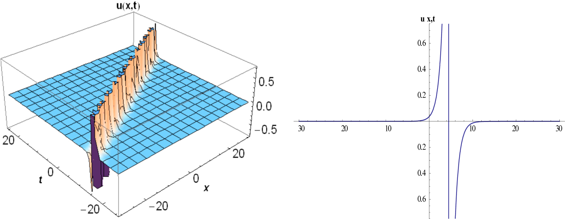
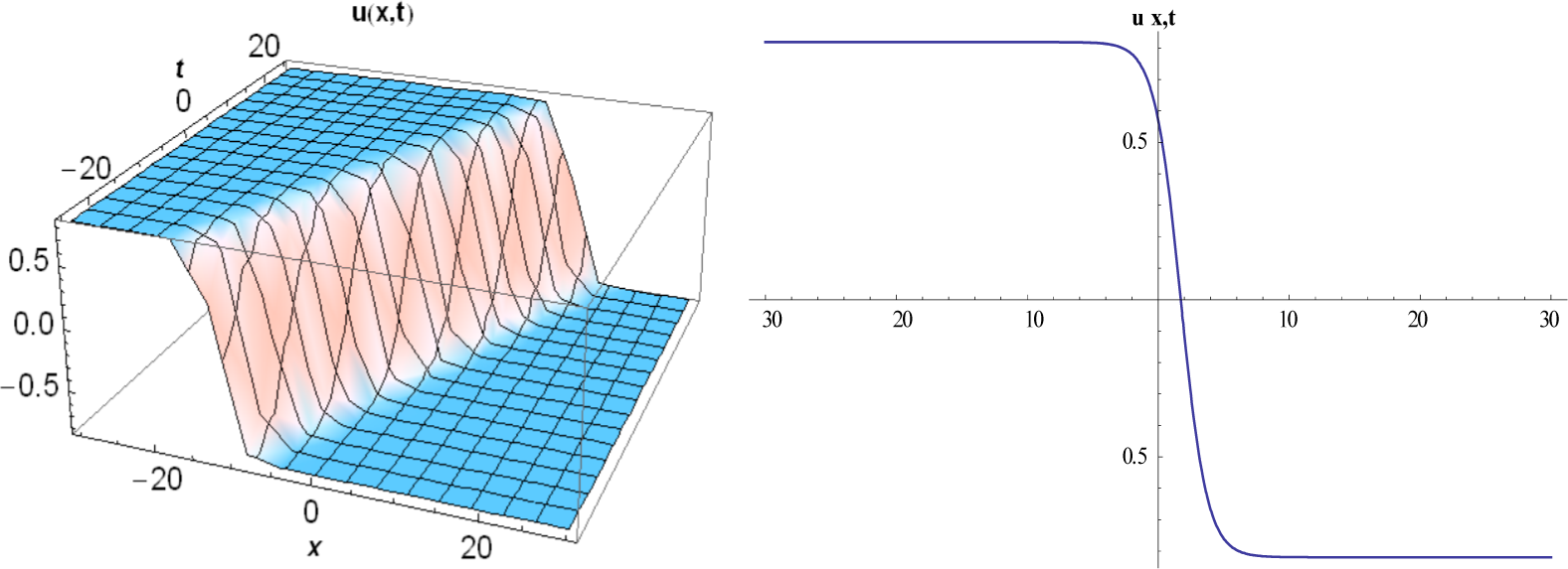
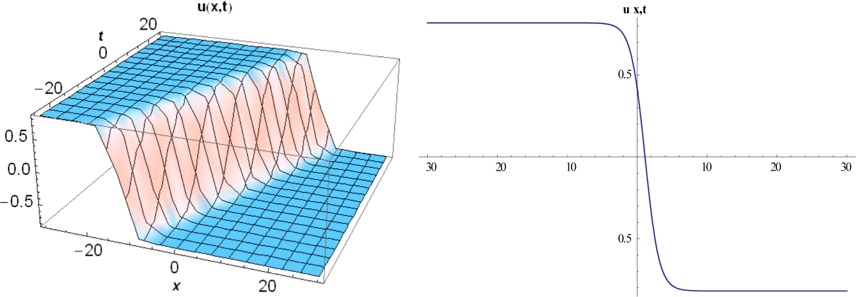
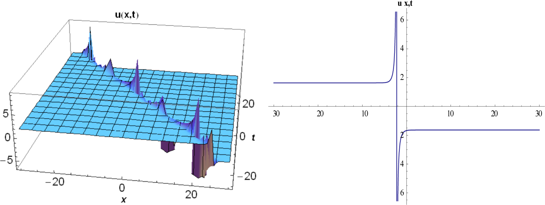
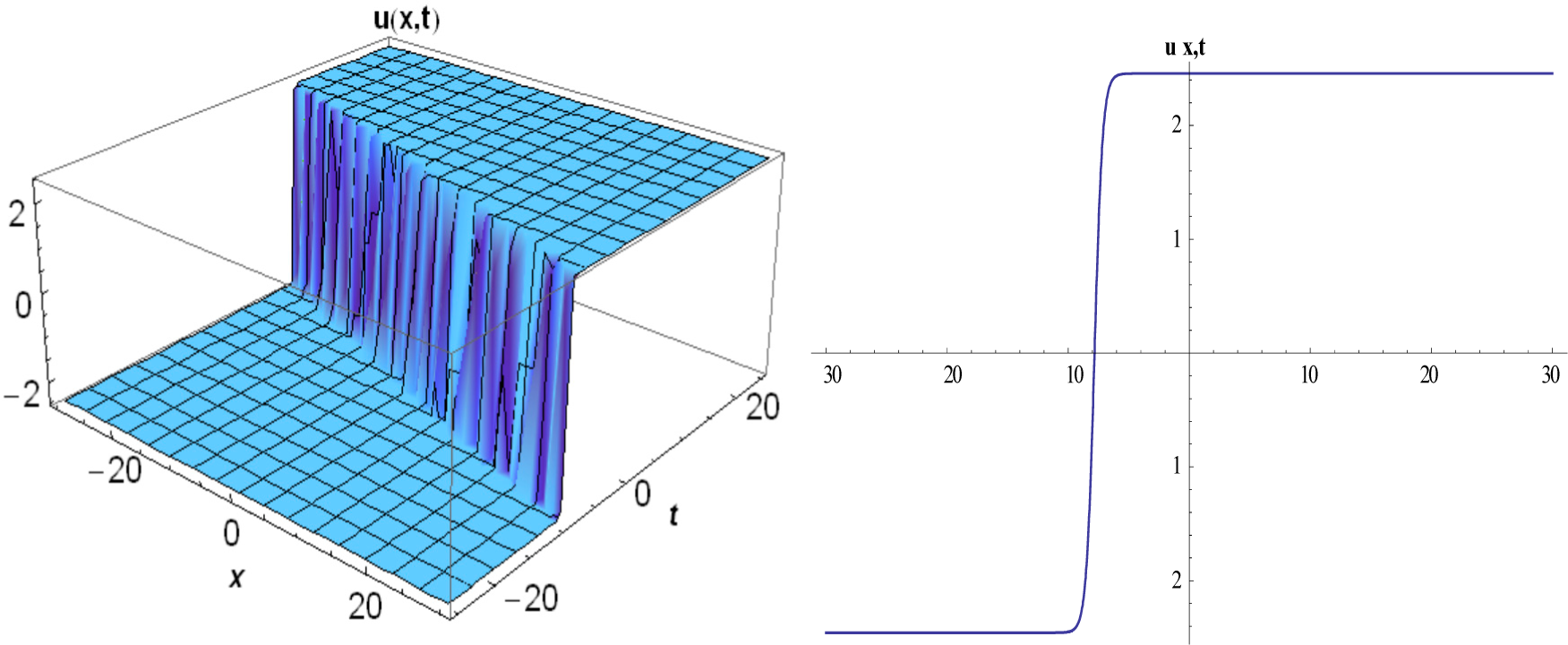
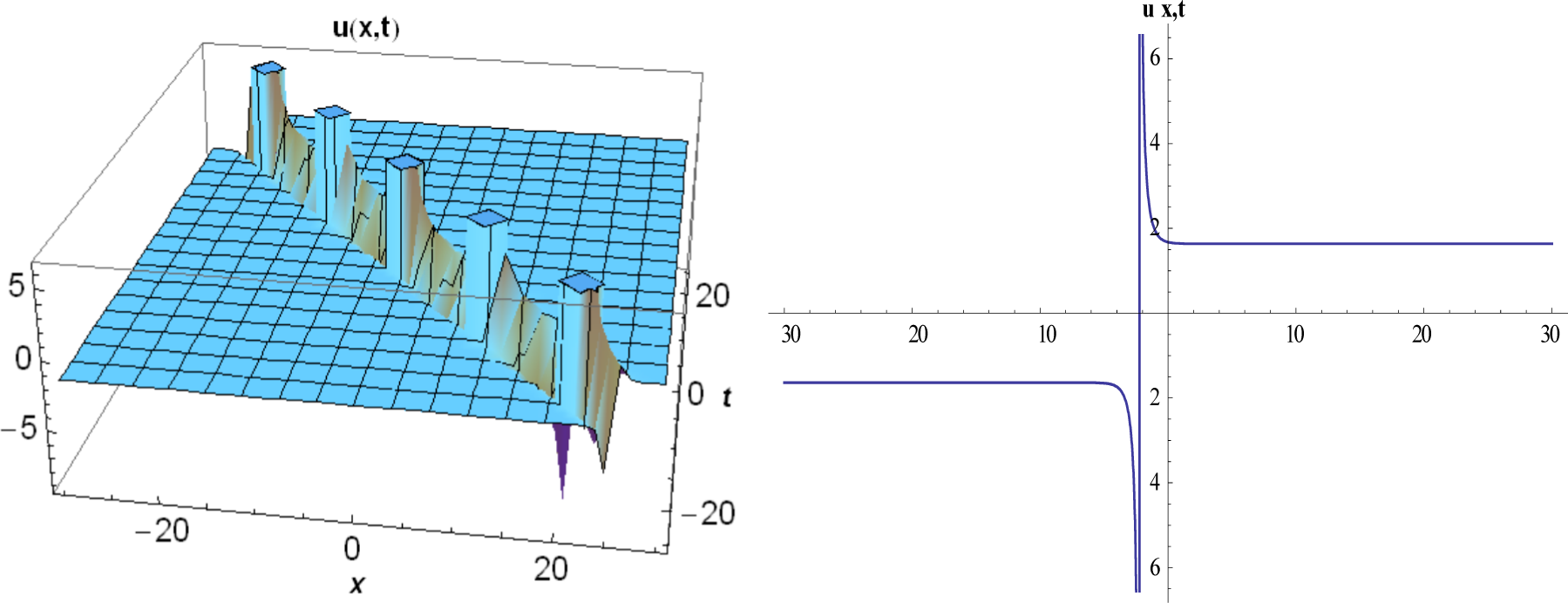
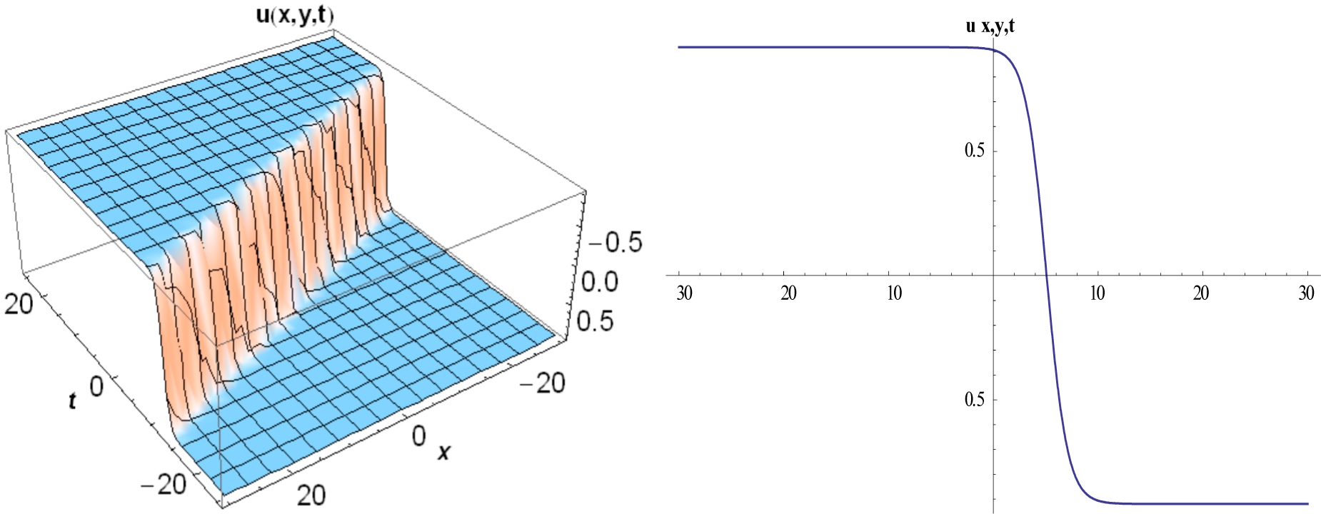
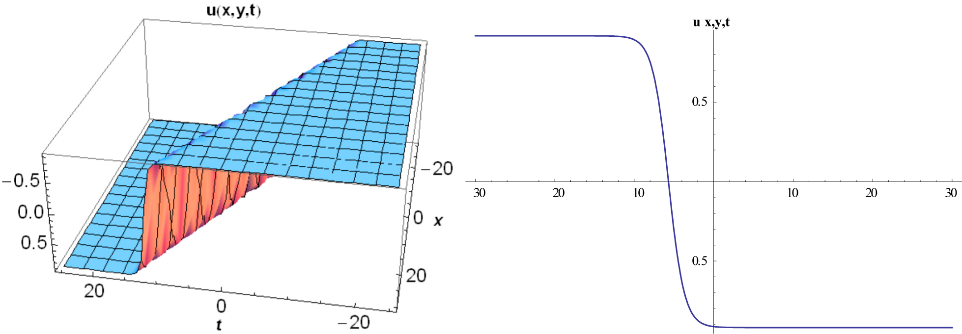
3. Implementation of Method Proposed

In this section, we have obtained the analytical solutions of the (1 + 1) dimensional nonlinear DMBBME and the (2 + 1)-dimensional nonlinear DMBBME cKGE by using GKM.
Example 1. Let’s consider the travelling wave solutions for the (1 + 1)-dimensional nonlinear DMBBME and we perform the travelling wave transformation u ( x , t ) = u ( η ) , η = x w t . When it comes to convert NLPDE into NLODE, we can get by carrying out the travelling wave transformation u ( x , t ) = u ( η ) to the Equation (1) as following:
u t = w u , u x = u , 3 u x 3 = u ,
being wis constant and not zero. Substituting Equation (11) into the Equation (1) by integrating with respect to η, we can find the NLODE for the (1 + 1)-dimensional nonlinear DMBBME:
3 u + 3 ( 1 w ) u α u 3 = 0 .
When we rearrange Equation (6) and Equation (9), with the help of balance principle, we obtain the term for suitability
N = M + 1 .
This resolution procedure is applied and we obtain results as follows:
Case 1: If we take M = 1 and N = 2 for Equation (6), then, we write following equalities:
u ( η ) = i = 0 2 a i Q i ( ρ ) j = 0 1 b j Q j ( ρ ) = a 0 + a 1 Q + a 2 Q 2 b 0 + b 1 Q
u ( η ) = ( Q 2 Q ) [ A B A B B 2 ] ,
and
u ( η ) = Q 2 Q B 2 [ ( 2 Q 1 ) ( A B A B ) + Q 2 Q B [ B ( A B A B ) 2 B A B + 2 A ( B ) 2 ] ]
where a 2 0 , b 1 0. When we use Equations (14) and (16) in Equation (12), we get a system of algebraic equations. By solving this system with the help of Wolfram Mathematica 9, we obtain the following coefficients;
a 0 = 0 , a 1 = 6 b 1 α , a 2 = 6 b 1 α , b 0 = b 1 2 , b 1 = b 1 , w = 2 ,
a 0 = 0 , a 1 = 6 b 1 α , a 2 = 6 b 1 α , b 0 = b 1 2 , b 1 = b 1 , w = 2 .
Substituting Equation (17) and Equation (18) into Equation (14) along with Q, we obtain the hyperbolic function solutions of the (1 + 1)-dimensional nonlinear DMBBME as following, respectively;
u 1 ( x , t ) = 6 α c o s e c h [ 2 t x ] ,
and
u 2 ( x , t ) = 6 α c o s e c h [ 2 t x ] .
Remark 1. The hyperbolic function solutions Equation (19) and Equation (20) obtained by using GKM are new analytical solutions when we compare it with the solutions obtained by Khan et al. [14]. These hyperbolic function solutions have been checked up whether they have verified the (1 + 1)-dimensional nonlinear DMBBME by Wolfram Mathematica 9.
Meanwhile, when the general properties of hyperbolic functions are considered, they can be written as complex trigonometric function solutions:
u 1 ( x , t ) = 6 α i c s c [ ( 2 t x ) i ] , u 2 ( x , t ) = 6 α i c s c [ ( 2 t x ) i ] .
To the best of our knowledge, the application of GKM in Equation (1) has not been submitted in the literature before. Figure 1, being the surfaces of complex trigonometric function solution Equation (19), was drawn by the same computer program. Of course, it is possible to see different surfaces of solutions according to various values of parameters.
Case 2: If we take M = 2 and N = 3 for Equation (6), then, we can write following equalities:
u ( η ) = i = 0 5 a i Q i ( ρ ) j = 0 2 b j Q j ( ρ ) = a 0 + a 1 Q + a 2 Q 2 + a 3 Q 3 b 0 + b 1 Q + b 2 Q 2 ,
u ( η ) = ( Q 2 Q ) [ A B A B B 2 ] ,
and
u ( η ) = Q 2 Q B 2 [ ( 2 Q 1 ) ( A B A B ) + Q 2 Q B [ B ( A B A B ) 2 B A B + 2 A ( B ) 2 ] ]
in which a 3 0 , b 2 0. When we use Equations (21) and (23) in Equation (12), we get a system of algebraic equations for Equation (12). By solving this system with the help of Wolfram Mathematica 9, we obtain the following coefficients:
Case 2.1:
a 0 = a 0 , a 1 = 4 α a 0 6 α b 1 2 + 8 a 0 b 2 α 6 α 2 α , a 3 = 0 , b 0 = a 0 2 α 3 , b 1 = b 1 , b 2 = b 2 , w = 1 2 , a 2 = 6 α ( b 1 + b 2 ) + 6 α b 1 2 + 8 a 0 b 2 α 6 α 2 α ,
Case 2.2:
a 0 = a 0 , a 1 = 2 a 0 b 1 3 2 α , a 2 = 3 ( 2 b 1 b 2 ) 2 α , a 3 = 6 b 2 α , b 0 = a 0 2 α 3 , b 1 = b 1 , b 2 = b 2 , w = 1 2 ,
Case 2.3:
a 0 = a 0 , a 1 = 2 a 0 + b 1 3 2 α , a 2 = 3 ( 2 b 1 + b 2 ) 2 α , a 3 = 6 b 2 α , b 0 = a 0 2 α 3 , b 1 = b 1 , b 2 = b 2 , w = 1 2 ,
Case 2.4:
a 0 = a 0 , a 1 = b 1 6 α , a 2 = 2 a 0 + 2 b 1 6 α , a 3 = 4 a 0 2 b 1 6 α , b 0 = a 0 α 3 , b 1 = b 1 , b 2 = 2 b 1 + 2 a 0 2 α 3 , w = 1 ,
Case 2.5:
a 0 = a 0 , a 1 = b 1 6 α , a 2 = 2 a 0 2 b 1 6 α , a 3 = 4 a 0 + 2 b 1 6 α , b 0 = a 0 α 6 , b 1 = b 1 , b 2 = 2 3 ( 3 b 1 + a 0 6 α ) , w = 1 ,
Case 2.6:
a 0 = a 0 , a 1 = 3 a 0 , a 2 = 3 a 0 , a 3 = 2 a 0 , b 0 = a 0 2 α 3 3 b 1 = a 0 2 α 3 , b 2 = a 0 2 α 3 , w = 7 2 ,
Case 2.7:
a 0 = a 0 , a 1 = 3 a 0 , a 2 = 3 a 0 , a 3 = 2 a 0 , b 0 = a 0 2 α 3 3 , b 1 = a 0 2 α 3 , b 2 = a 0 2 α 3 , w = 7 2 ,
Case 2.8:
a 0 = a 0 , a 1 = 0 , a 2 = 2 a 0 , a 3 = 4 a 0 , b 0 = a 0 α 6 , b 1 = 0 , b 2 = 2 a 0 2 α 3 , w = 1 ,
Case 2.9:
a 0 = a 0 , a 1 = 0 , a 2 = 2 a 0 , a 3 = 4 a 0 , b 0 = a 0 α 6 , b 1 = 0 , b 2 = 2 a 0 2 α 3 , w = 1 .
Substituting Equations (24)(32) into Equation (14) along with Q, we can obtain some new analytical solutions to the (1 + 1)-dimensional nonlinear DMBBME as the following, respectively.
For Case 2.1, we can find the rational exponential function solution to Equation (1) as following:
u 3 ( x , t ) = 6 α a 0 ( e t e 2 x ) 3 6 α e t ( b 1 + b 2 ) + 3 e x + t 2 6 α b 1 2 + 8 α a 0 b 2 6 α 2 α a 0 6 α ( e x + e t 2 ) 2 6 α e x + t 2 6 α e t ( b 1 + b 2 ) ,
For Case 2.2 and Case 2.3, we can obtain another hyperbolic function solution to Equation (1):
u 4 ( x , t ) = 3 2 α tanh ( 1 4 ( t 2 x ) ) ,
For Case 2.4 and Case 2.5, another rational exponential function solution to Equation (1) is found in the following manner:
u 5 ( x , t ) = 6 ( 1 + e 2 x + 2 t ) ( a 0 α ( 3 + e x + t ) b 1 6 ) α ( 1 + e 2 x + 2 t ) ( a 0 6 α ( 3 + e x + t ) 6 b 1 ) ,
For Case 2.6 and Case 2.7, we can attain new complex trigonometric function solution to Equation (1):
u 6 ( x , t ) = 3 3 2 α [ i tan ( 3 4 ( 7 t + 2 x ) i ) ] ,
For Case 2.8 and Case 2.9, we can get another new complex trigonometric function solution to Equation (1):
u 7 ( x , t ) = 6 α [ i cot ( x i + t i ) ] .
Remark 2. Travelling wave solutions, Equations (33) and (35)(37), obtained by using GKM are new analytical solutions to the (1 + 1)-dimensional nonlinear DMBBME and analytical solution, Equation (34), is the same as the solution of Khan et al. [14]. We have checked up whether they have verified the (1 + 1)-dimensional nonlinear DMBBME with the help of Wolfram Mathematica 9. Then, Figures 26 were drawn by the same program. To the best of our knowledge, the application of GKM to Equation (1) has not been submitted to the literature before.
Example 2. Let us consider the (2 + 1)-dimensional nonlinear cKGE defined by:
u x x + u y y u t t + α u + β u 3 = 0 , α < 0 , β 0 ,
in which α , β coefficients are constants and not zero [15]. When it comes to convert Equation (38) into NLODE, we can perform the travelling wave transformation:
u ( x , y , t ) = u ( η ) , η = k ( x + y c t ) , 2 u x 2 = k 2 u , 2 u y 2 = k 2 u , 2 u t 2 = k 2 c 2 u ,
in which k and c are constants and not zero. Substituting Equation (39) into Equation (38), we find the NLODE for the (2 + 1)-dimensional nonlinear cKGE:
( 2 c 2 ) k 2 u + α u + β u 3 = 0 .
When we rearrange Equation (6) and Equation (9), we obtain a relationship between Nand M with the help of balance principle as following;
N = M + 1 .
Case 1: If we take M = 1 and N = 2 for Equation (6), then, we can write following equalities;
u ( η ) = i = 0 2 a i Q i ( ρ ) j = 0 1 b j Q j ( ρ ) = a 0 + a 1 Q + a 2 Q 2 b 0 + b 1 Q ,
u ( η ) = ( Q 2 Q ) [ A B A B B 2 ] ,
and
u ( η ) = Q 2 Q B 2 [ ( 2 Q 1 ) ( A B A B ) + Q 2 Q B [ B ( A B A B ) 2 B A B + 2 A ( B ) 2 ] ]
in which a 2 0 , b 1 0 and are constants. When we use Equations (42) and (44) in Equation (40), we find a system of algebraic equations. Solving system of algebraic equations using Wolfram Mathematica 9, it gives us the following coefficients:
Case 1.1.
a 0 = b 0 α β , a 1 = α ( 2 b 0 + b 1 ) β , a 2 = 2 α b 1 β , b 0 = b 0 , b 1 = b 1 , c = 2 2 α ,
Case 1.2.
a 0 = b 0 α β , a 1 = α ( 2 b 0 + b 1 ) β , a 2 = 2 α b 1 β , b 0 = b 0 , b 1 = b 1 , c = 2 2 α ,
Case 1.3.
a 0 = b 0 α β , a 1 = α ( 2 b 0 + b 1 ) β , a 2 = 0 , b 0 = b 0 , b 1 = b 1 , c = 2 2 α ,
Case 1.4.
a 0 = b 0 α β , a 1 = α ( 2 b 0 + b 1 ) β , a 2 = 0 , b 0 = b 0 , b 1 = b 1 , c = 2 2 α ,
Case 1.5.
a 0 = b 0 α β , a 1 = α ( 2 b 0 + b 1 ) β , a 2 = 2 b 1 α β , b 0 = b 0 , b 1 = b 1 , c = 2 2 α ,
Case 1.6.
a 0 = b 0 α β , a 1 = α ( 2 b 0 + b 1 ) β , a 2 = 2 b 1 α β , b 0 = b 0 , b 1 = b 1 , c = 2 2 α .
First of all, substituting Equation (45) and Equation (46) into Equation (42) along with Q, we attain the hyperbolic function solution for the (2 + 1)-dimensional nonlinear cKGE:
u 1 ( x , y , t ) = α β tanh ( x + y t 2 2 α 2 ) .
Secondly, substituting Equation (47) and Equation (48) in Equation (42) along with Q, we obtain the new rational function solution for the (2 + 1)-dimensional nonlinear cKGE:
u 2 ( x , y , t ) = b 0 α e x + y ( b 0 + b 1 ) α e t 2 2 α b 0 β e x + y ( b 0 + b 1 ) β e t 2 2 α .
Finally, when we use Equation (49) and Equation (50) in Equation (42) along with Q, we obtain the new complex trigonometric function solution for Equation (2):
u 3 ( x , y , t ) = α β [ i tan ( 1 2 i ( x + y + t 2 2 α ) ) ] .
Remark 3. The travelling wave solution, Equation (51), obtained using GKM, is the same as the solution found by Khan et al. [15]. The analytical solutions, Equations (52) and (53), obtained using GKM, are new rational function solution and complex trigonometric function solution for the (2 + 1)-dimensional nonlinear cKGE. We have checked up whether these analytical solutions, Equations (51)(53), have verified the (2 + 1)-dimensional nonlinear cKGE with the same computer program. Figures 79 were drawn by the same computer program. To the best of our knowledge, analytical solutions, Equations (52) and (53), have not been submitted to the literature before.

4. Conclusions

In this present manuscript, we have applied the GKM to the (1 + 1)-dimensional nonlinear DMBBME and the (2 + 1)-dimensional nonlinear cKGE. Then, we obtained some new analytical solutions, such as complex trigonometric function, trigonometric function, and hyperbolic function solutions. We have proven that they have been verified Equation (1) and Equation (2) by using Wolfram Mathematica 9.
Under the terms of this information, it has been observed that GKM has been a powerful tool to obtain the analytical solutions of such differential equations. We think that this method can also be conducted on other nonlinear partial differential equations.

5. Discussions and Comparisons

Ma and Fuchssteiner have already submitted to the literature a study including systematical approaches to travelling wave solutions including analytical function solutions such as tangent hyperbolic function, rational function and trigonometric function solutions of general Riccati equation [12].
We have obtained the tangent hyperbolic function solution u 4 ( x , t ), hyperbolic function solutions such as u 1 ( x , t ) and u 2 ( x , t ) , exponential rational function solutions such as u 3 ( x , t ) and u 5 ( x , t ) and complex trigonometric function solutions such as u 6 ( x , t ) and u 7 ( x , t )for the (1 + 1)-dimensional nonlinear DMBBME by using GKM, which is a special case of the transformed rational function method [8].
Moreover, we have achieved the tangent hyperbolic function solution u 1 ( x , y , t ), exponential rational function solution u 2 ( x , y , t )and complex trigonometric function solution u 3 ( x , y , t )for the (2 + 1)-dimensional nonlinear cKGE by the same method.
Another powerful side of this method is that it has many solution formats found by considering the balance rule. We have considered only two cases in this paper. If we take other values of Nand M , of course, it is possible to obtain more analytical solutions for such differential equations. This is not finite.
When it comes to general properties of these equations, as in Section 3, we have converted both problems into homogeneous nonlinear second order ordinary differential equations, such as Equations (12) and (40) in this paper. Uniqueness and existence of nonlinear second order ordinary differential equations, which are Equations (12) and (40), have already been submitted to the literature by Baxley [33].
Some authors have studied the general properties of the Generalized Benjamin–Bona–Mahony equation such as existence, uniqueness for periodic solutions and the stability of travelling wave solutions. Olver has investigated the conservation laws of the Benjamin–Bona–Mahony equation [34]. Johnson has studied the stability of periodic solutions of the generalized Benjamin–Bona–Mahony equation [35]. Zeng has worked on existence and stability of solitary-wave solutions of equations of Benjamin–Bona–Mahony type [36]. Medeiros et al. have submitted an article titled Existence and Uniqueness for Periodic Solutions of the Benjamin–Bona–Mahony Equation [37].
The normal forms and global existence of solutions of nonlinear cKGE have already been submitted to the literature by Moriyama [38]. Selberg and Tesfahun have investigated unconditional uniqueness for the Dirac–Klein–Gordon equations in two space dimensions [39].

Acknowledgments

The authors would like to thank the reviewers for their comments that help improve the manuscript.

Author Contributions

All authors have read and approved the final manuscript.

Conflicts of Interest

The authors declare no conflict of interest.

References

  1. Liu, C.S. Trial Equation Method and its Applications to Nonlinear Evolution Equations. Acta Phys. Sin. 2005, 54, 2505–2509. [Google Scholar]
  2. Liu, C.S. A New Trial Equation Method its Applications, Communications in Theoretical Physics. Commun. Theor. Phys. 2006, 45, 395–397. [Google Scholar]
  3. Liu, C.S. Trial Equation Method for Nonlinear Evolution Equations with Rank Inhomogeneous: Mathematical Discussions and Applications. Commun. Theor. Phys. 2006, 45, 219–223. [Google Scholar]
  4. Bulut, H.; Baskonus, H.M.; Pandir, Y. The Modified Trial Equation Method for Fractional Wave Equation and Time-Fractional Generalized Burgers Equation. Abstr. Appl. Anal. 2013, 2013, 636802. [Google Scholar]
  5. Zayed, E.M.E.; Abdelaziz, M.A.M. Exact Solutions for the Nonlinear Schrödinger Equation with Variable Coefficients Using the Generalized Extended Tanh-Function, the Sine-Cosine and the Exp-function Methods. Appl. Math. Comput. 2011, 218, 2259–2268. [Google Scholar]
  6. Wazwaz, A. M. The Tanh Method: Solitons and Periodic Solutions for Dodd–Bullough–Mikhailov and Tzitzeica–Dodd–Bullough Equations. Chaos Solitons Fractals 2005, 25, 55–56. [Google Scholar]
  7. Khan, K.; Ali Akbar, M. Traveling Wave Solutions of the (2 + 1)-Dimensional Zoomeron Equation and the Burgers Equations via the MSE Method and the Exp-function Method. Ain Shams Eng. J. 2014, 5, 247–256. [Google Scholar]
  8. Ma, W.X.; Lee, J.H. A Transformed Rational Function Method and Exact Solutions to the 3 + 1 Dimensional Jimbo–Miwa Equation. Chaos Solitons Fractals 2009, 42, 1356–1363. [Google Scholar]
  9. Ma, W.X.; Huang, T.W.; Zhang, Y. A Multiple Exp-function Method for Nonlinear Differential Equations and its Application. Phys. Scr. 2010, 82, 065003. [Google Scholar]
  10. Ma, W.X.; Zhu, Z.N. Solving the (3+1)-Dimensional Generalized KP and BKP Equations by the Multiple Exp-function Algorithm. Appl. Math. Comput. 2012, 218, 11871–11879. [Google Scholar]
  11. Ma, W.X. Generalized Bilinear Differential Equations. Stud. Nonlinear Sci. 2011, 2, 140–144. [Google Scholar]
  12. Ma, W.X.; Fuchssteiner, B. Explicit and Exact Solutions to a Kolmogorov–Petrovskii–Piskunov Equation. Int. J. Nonlinear Mech. 1996, 31, 329–338. [Google Scholar]
  13. Ma, W.X.; Wu, H.Y.; He, J.S. Partial Differential Equations Possessing Frobenius Integrable Decompositions. Phys. Lett. A 2007, 364, 29–32. [Google Scholar]
  14. Khan, K.; Ali Akbar, M.; Rayhanul Islam,, S.M. Exact Solutions for (1 + 1)-Dimensional Nonlinear Dispersive Modified Benjamin–Bona–Mahony Equation and Coupled Klein–Gordon Equations. SpringerPlus 2014, 3. [Google Scholar] [CrossRef]
  15. Khan, K.; Ali Akbar, M. Exact Solutions of the (2+1)-Dimensional Cubic Klein–Gordon Equation and the (3+1)-Dimensional Zakharov–Kuznetsov Equation Using the Modified Simple Equation Method. J. Assn. Arab Univ. Basic Appl. Sci. 2014, 15, 74–81. [Google Scholar]
  16. Benjamin–Bona–Mahony Equation. Available online: http://en.wikipedia.org/wiki/Benjamin%E2%80%93Bona%E2%80%93Mahony_equation accessed on 1 February 2015.
  17. Yusufoglu, E. New Solitary Solutions for the MBBM Equations Using Exp-function Method. Phys. Lett. 2008, 372, 442–446. [Google Scholar]
  18. Eme, Z.; Al-Joudi, S. Applications of an Extended (G’/G)-Expansion Method to Find Exact Solutions of Nonlinear PDEs in Mathematical Physics. Math. Probl. Eng. 2010, 2010, 768573. [Google Scholar]
  19. Klein–Gordon Equation. Available online: https://en.wikipedia.org/wiki/Klein%E2%80%93Gordon_equation accessed on 1 February 2015.
  20. Evans, L.C. Entropy and Partial Differential Equations. 2004. Available online: https://math.berkeley.edu/~evans/entropy.and.PDE.pdf accessed on 19 June 2015.
  21. Jüngel, A. Entropy Dissipation Methods for Nonlınear Partial Differentıal Equations; Lecture Notes; Spring School: Bielefeld, March 2012. Available online: http://www.asc.tuwien.ac.at/~juengel/scripts/Bielefeld1203.pdf accessed on 19 June 2015.
  22. Parsani, M.; Carpenter, M.H.; Nielsen, E.J. Entropy Stable Wall Boundary Conditions for the Three-Dimensional Compressible Navier–Stokes Equations. J. Comput. Phys. 2015, 292, 88–113. [Google Scholar]
  23. Zhao, Y.; Yuan, M.; Su, G.; Chen, T. Crowd Macro State Detection Using Entropy Model. Physica A 2015, 431, 84–93. [Google Scholar]
  24. Elling, V. Relative Entropy and Compressible Potential Flow. Acta. Math. Sci. 2015, 35, 763–776. [Google Scholar]
  25. Chen, S.; Yang, B.; Xiao, X.; Zheng, C. Analysis of Entropy Generation in Double-Diffusive Natural Convection of Nano fluid. Int. J. Heat Mass Tran. 2015, 87, 447–463. [Google Scholar]
  26. Lv, Y.; Ihme, M. Entropy-Bounded Discontinuous Galerkin Scheme for Euler Equations. J. Comput. Phys. 2015, 295, 715–739. [Google Scholar]
  27. Broadbridge, P. Entropy Diagnostics for Fourth Order Partial Differential Equations in Conservation Form. Entropy 2008, 10, 365–379. [Google Scholar]
  28. Kudryashov, N.A. One Method for Finding Exact Solutions of Nonlinear Differential Equations. Commun. Nonlinear Sci. Numer. Simul. 2012, 17, 2248–2253. [Google Scholar]
  29. Lee, J.; Sakthivel, R. Exact Travelling Wave Solutions for some Important Nonlinear Physical Models. Pramana 2013, 80, 757–769. [Google Scholar]
  30. Ryabov, P.N.; Sinelshchikov, D.I.; Kochanov, M.B. Application of the Kudryashov Method for Finding Exact Solutions of the High Order Nonlinear Evolution Equations. Appl. Math. Comput. 2011, 218, 3965–3972. [Google Scholar]
  31. Demiray, S.T.; Pandir, Y.; Bulut, H. Generalized Kudryashov Method for Time-Fractional Differential Equations. Abstr. Appl. Anal. 2014, 2014, 901540. [Google Scholar]
  32. Çimen, T. On the Existence of Solutions Characterized by Riccati Equations to Infinite-Time Horizon Nonlinear Optimal Control Problems. Proceeding of The 18th IFAC World Congress, Milano, Italy, 28 August–2 September 2011; pp. 9616–9626.
  33. Baxley, J.V. Existence Theorems for Nonlinear Second Order Boundary Value Problems. J. Differ. Equ. 1990, 85, 125–150. [Google Scholar]
  34. Olver, P.J. Euler Operators Conservation Laws of the BBM Equation. Math. Proc. Camb. Phil. Soc. 1979, 85, 143–160. [Google Scholar]
  35. Johnson, M.A. On the Stability of Periodic Solutions of the Generalized Benjamin–Bona–Mahony Equation. Physica D 2010, 239, 1892–1908. [Google Scholar]
  36. Zeng, L. Existence and Stability of Solitary-Wave Solutions of Equations of Benjamin–Bona–Mahony Type. J. Differ. Equ. 2003, 188, 1–32. [Google Scholar]
  37. Medeiros, L.A.; Perla Menzala, G. Existence and Uniqueness for Periodic Solutions of the Benjamin–Bona–Mahony Equation. SIAM J. Math. Anal. 1977, 8, 792–799. [Google Scholar]
  38. Moriyama, K. Normal Forms and Global Existence of Solutions to a Class of Cubic Nonlinear Klein–Gordon Equations in one Space Dimension. Differ. Integr. Equ. 1997, 10, 499–520. [Google Scholar]
  39. Selberg, S.; Tesfahun, A. Unconditional Uniqueness in the Charge Class for the Dirac–Klein–Gordon Equations in two Space Dimensions. Nonlinear Differ. Equ. Appl. 2013, 20, 1055–1063. [Google Scholar]
Figure 1. The 3D and 2D graphs of the hyperbolic function solution Equation (19) by considering the values 30 < x < 30 , α = 5 , 25 < t < 25 , for 3D graphics and t = 5for 2D graphics.
Entropy 17 04255f1
Figure 2. The 3D and 2D graphs of the analytical solution Equation (33) by considering the values α = 5 , a 0 = 2 , b 1 = 3 , b 2 = 7 , 30 < x < 30 , 25 < t < 25 , for 3D graphics and t = 5 for 2D graphics.
Entropy 17 04255f2
Figure 3. The 3D and 2D graphs of the analytical solution Equation (34) by considering the values α = 5 , 30 < x < 30 , 25 < t < 25 , for 3D graphics and t = 5 for 2D graphics.
Entropy 17 04255f3
Figure 4. The 3D and 2D graphs of the analytical solution Equation (35) by considering the values α = 5 , a 0 = 2 , b 1 = 3 , 30 < x < 30 , 25 < t < 25 , for 3D graphics and t = 5 for 2D graphics.
Entropy 17 04255f4
Figure 5. The 3D and 2D graphs of the analytical solution Equation (36) by considering the values α = 5 , 30 < x < 30 , 25 < t < 25 , for 3D graphics and t = 5 for 2D graphics.
Entropy 17 04255f5
Figure 6. The 3D and 2D graphs of the analytical solution Equation (37) by considering the values α = 5 , 30 < x < 30 , 25 < t < 25 , for 3D graphics and t = 5 for 2D graphics.
Entropy 17 04255f6
Figure 7. The 3D and 2D graphs of the analytical solution Equation (51) by considering the values 30 < x < 30 , 25 < t < 25 , α = 5 , β = 7 , y = 3 / 5 , for 3D graphics and t = 5 for 2D surface.
Entropy 17 04255f7
Figure 8. The 3D and 2D graphs of the rational function solution Equation (52) by considering the values 30 < x < 30 , 25 < t < 25 , α = 5 , β = 7 , y = 3 / 5 , b 0 = 3 , b 1 = 2 for 3D graphics and t = 5 for 2D graphics.
Entropy 17 04255f8
Figure 9. The 3D and 2D graphs of the analytical solution Equation (53) by considering the values 30 < x < 30 , 25 < t < 25 , α = 5 , β = 7 , y = 3 / 5 , for 3D graphics and t = 5 for 2D surface.
Entropy 17 04255f9

