Spectral Embedded Deep Clustering
by
 ,
,
Yuichiro Wada
1, 
Shugo Miyamoto
2,
Takumi Nakagama
3,
Léo Andéol
4,5,
Wataru Kumagai
5 and
Takafumi Kanamori
3,5,* 1
Graduate School of Information Science, Nagoya University, Furo-cho, Chikusa-ku, Nagoya 464-8601, Japan
2
Department of Systems Innovation, School of Engineering, The University of Tokyo, Hongo Campus, Eng. Bldg. No. 3, 2F, 7-3-1 Hongo, Bunkyo-ku, Tokyo 113-8656, Japan
3
Department of Mathematical and Computing Science, School of Computing, Tokyo Institute of Technology, 2-12-1 Ookayama, Meguro-ku, Tokyo 152-8552, Japan
4
Computer Science Department, Sorbonne Université, 4 place Jussieu, 75005 Paris, France
5
RIKEN AIP, Nihonbashi 1-chome Mitsui Building, 15th floor, 1-4-1 Nihonbashi, Chuo-ku, Tokyo 103-0027, Japan
*
Author to whom correspondence should be addressed.
Entropy 2019, 21(8), 795; https://doi.org/10.3390/e21080795
Submission received: 13 June 2019
/
Revised: 4 August 2019
/
Accepted: 12 August 2019
/
Published: 15 August 2019
Abstract
:We propose a new clustering method based on a deep neural network. Given an unlabeled dataset and the number of clusters, our method directly groups the dataset into the given number of clusters in the original space. We use a conditional discrete probability distribution defined by a deep neural network as a statistical model. Our strategy is first to estimate the cluster labels of unlabeled data points selected from a high-density region, and then to conduct semi-supervised learning to train the model by using the estimated cluster labels and the remaining unlabeled data points. Lastly, by using the trained model, we obtain the estimated cluster labels of all given unlabeled data points. The advantage of our method is that it does not require key conditions. Existing clustering methods with deep neural networks assume that the cluster balance of a given dataset is uniform. Moreover, it also can be applied to various data domains as long as the data is expressed by a feature vector. In addition, it is observed that our method is robust against outliers. Therefore, the proposed method is expected to perform, on average, better than previous methods. We conducted numerical experiments on five commonly used datasets to confirm the effectiveness of the proposed method.
1. Introduction
Clustering is one of the oldest machine-learning fields, where the objective is, given data points, to group them into clusters according to some measure. Many clustering methods have been proposed for a long while [1], and been applied to real-world problems [2].
The best known classical methods are k-means [3] and Gaussian Mixture Model (GMM) clustering [4]. Though those methods are computationally efficient, they can only model convex shapes and are thus applicable in limited cases. The kernel k-means [5], kernel GMM clustering [6] and Spectral Clustering (SC) [7] can capture more complicated shapes than k-means and GMM but are difficult to scale up to large datasets. In recent years, due to technological progress, we can acquire many types of data such as images, texts, and genomes in large numbers. Thus, the demand of advanced efficient clustering methods grows even stronger [8].
Thanks to the development of deep neural networks, we can now handle large datasets with complicated shapes [9]. Consequently, the studies of clustering using deep neural networks has been proposed. One major direction in the studies is to combine deep AutoEncoders (AE) [10] with classical clustering methods. This AE is used to obtain a clustering friendly low dimensional representation. Another major direction is directly grouping a given unlabeled dataset into the clusters in the original input space by employing a deep neural network to model the distribution of cluster labels.
With both directions, there exist popular methods. We summarize their applicable data domain and well performing condition in Table 1. For examples, CatGAN (Categorical Generative Adversarial Networks) learns discriminative neural network classifiers that maximize mutual information between the input data points and the cluster labels, while enforcing the robustness of the classifiers to data points produced by adversarial generative models. Since maximizing mutual information implicitly encourages the cluster-balance distribution of the model to be uniform, CatGAN performs well under the condition of the uniform cluster balance. JULE (Joint Unsupervised LEarning) learns a clustering friendly low dimensional representation for image datasets by using a convolutional neural network [11]. The assigned cluster labels and low dimensional representation are jointly optimized by updating a similarity matrix of the representations, where n is the number of data points. Thus, memory space must be secured to conduct the method.
As we can see in Table 1, most of their key conditions are not always realistic since the details of given unlabeled datasets are unknown and their size is large in typical machine-learning scenarios. On the other hand, SpectralNet does not require key condition. It only requires the following two fundamental assumptions: the smoothness and manifold assumptions [18]. Please note that the other methods in Table 1 also require the two assumptions. As for the weakness of SpectralNet, it is not robust against outliers. In the learning process, it learns the pairwise similarities over all data points. Therefore, the existence of outliers disturbs the method learning the similarities precisely, and thus returns inaccurate clustering results.
In this paper, we propose a deep clustering method named Spectral Embedded Deep Clustering (SEDC). Given an unlabeled dataset and the number of clusters, SEDC directly groups the dataset into the given number clusters in the input space. Our statistical model is the conditional discrete probability distribution, which is defined by a fully connected deep neural network. SEDC does not require key condition except the smoothness and manifold assumptions, and it can be applied to various data domains. Moreover, throughout our numerical experiments, we observed that our method was more robust against outliers than SpectralNet.
The procedure of SEDC is composed of two stages. In the first stage, we conduct SC only on the unlabeled data points selected from high-density region by using the geodesic metric to estimate the cluster labels. This special type of SC is named as Selective Geodesic Spectral Clustering (SGSC), which we propose for assisting SEDC as well. Thereafter, we conduct semi-supervised learning to train the model by using the estimated cluster labels and the remaining unlabeled data points. Please note that in this semi-supervised learning, we treat the estimated cluster labels of the selected unlabeled data points as the given true cluster labels. At last, by using the trained model, we obtain the estimated cluster labels of all given unlabeled data points.
2. Related Works
In this section, we first introduce the existing clustering studies based on deep neural networks. As mentioned in Section 1, there are two major directions in recent studies, i.e., the deep-AE-based clustering and the direct deep clustering. We then introduce the two techniques related to our proposed method, i.e., SC and Virtual Adversarial Training (VAT).
2.1. Existing Clustering Methods Using Deep Neural Network
In deep-AE-based clustering, the AE and a classical clustering method such as k-means are combined. The combination strategies are either sequential [19,20] or simultaneous [12,13,14]. In the sequential way, deeply embedded representations of the given dataset are obtained by the deep AE, and then a classical clustering method is applied to the embedded set. In the simultaneous way, the deep representations and their cluster labels are learned jointly by optimizing a single objective function.
As examples of the simultaneous way, we introduce [12,14] here. The method of [12] is named Deep Embedded Clustering (DEC). DEC trains a deep neural network by iteratively minimizing the Kullback–Leibler (KL) divergence between a centroid-based probability distribution and an auxiliary target distribution. The deep network is used as the AE. They reported the clustering performance of DEC depended on the initial embedded representations and cluster centroids obtained by the AE and k-means. The method of [14] is named Variational Deep Embedding (VaDE). The approach relies on a Variational AutoEncoder (VAE) [21] that uses a Gaussian mixture prior. VaDE trains its deep neural network by minimizing the reconstruction error, while enforcing that the low dimensional representations follow the Gaussian mixture model.
Regarding the direct deep clustering, we introduce [15,17]. The method of [15] is named Information Maximizing Self-Augmented Training (IMSAT). It is based on data augmentation, where a deep neural network is trained to maximize the mutual information while regularizing the network so that the cluster label assignment of original data will be consistent with the assignment of augmented data. The method of [17] is named SpectralNet. This method is proposed to overcome the scalability and generalization of SC. It uses two deep neural networks. The first network learns the similarities among all given data points. This network is known as Siamese net [22]. Then, the second network learns a dimension reduction mapping which preserves the similarities obtained by the first net. After both are trained, the dimensionality reduced data points obtained by the second network are grouped into clusters by k-means.
2.2. Related Techniques with Proposed Method
SEDC handles the following clustering problem: given a set of unlabeled data points () and the number of clusters C, group into C clusters. In SEDC, the estimated cluster label of is obtained by the trained conditional discrete probability distributional classifier. This classifier is denoted by where , and y are a set of parameters, a feature vector and a cluster label, respectively. The cluster label y ranges . In addition, the classifier is defined by a fully connected deep neural network whose last layer is the soft-max function. SC and VAT, explained below, take an important role in SEDC: see the detail in Section 3.
2.2.1. Spectral Clustering
SC [7,23] is a popular classical clustering algorithm. We here introduce the commonly used framework of SC, which is used also in SEDC algorithm. It first embeds the data points in the eigenspace of the Laplacian matrix derived from the pairwise similarities over all given data points. Then, SC applies k-means on the representation to obtain the cluster labels. The SC algorithm is outlined below.
Given dataset , define the weighted undirected graph G which comprises a set of vertices and a set of undirected edges E defined by -nearest neighbor (-NN) based on a metric d. Suppose that each edge has a non-negative symmetric weight .
Denote the affinity matrix on G by , where , and is the diagonal matrix whose entries are given by .
Given the number of clusters C, compute the largest C eigenvectors of the eigenproblem . Let be the matrix containing the vectors as columns. Thereafter, re-normalize each row of to have unit length.
Cluster n rows of as points in by conducting k-means (k ). Let and be the estimated labels of and the set of centroids obtained by k-means, respectively.
The above procedure can be noted as . The weight w is often defined by the following similarity function:
2.2.2. Virtual Adversarial Training
VAT [26] is a regularization method based on local perturbation. It forces the statistical model follow the smoothness assumption. VAT is known to empirically perform better than other local perturbation methods such as random perturbation [27] and adversarial training [28] in both semi-supervised and supervised learning scenarios. It can be employed also in unsupervised learning scenarios [15,29] since VAT only requires the unlabeled data points.
VAT first defines the adversarial point with given as follows:
where is -perturbation to a virtual adversarial direction:
In Equation (3), is the estimated parameter at t-th iteration, and is Kullback–Leibler divergence [30]. Then, VAT minimizes the following with respect to :
3. Proposed Method
As we already mentioned in the end of Section 1 and the beginning of Section 2.2, given an unlabeled dataset () and the number of clusters C, our proposed deep clustering named SEDC groups into C clusters. Since this grouping is achieved by obtaining the estimated cluster labels of , our goal can be replaced by estimating the cluster labels up to permutation of labels. In SEDC, the estimated cluster label of each is defined by , where is the trained set of parameters. The training scheme of the classifier is as follows: we firstly only estimate the cluster labels of selected unlabeled data points by using only (this part is done by SGSC algorithm.), and then conduct semi-supervised learning to train the classifier. Regarding with this semi-supervised learning, we use the estimated cluster labels of selected unlabeled data points and the remaining unlabeled data points, which are treated as the given true cluster labels and unlabeled data points respectively.
In this section, we first introduce SGSC. Thereafter, we present our main method SEDC.
3.1. Selective Geodesic Spectral Clustering
Using SGSC, the clustering problem is converted into a semi-supervised learning problem as shown below. In SGSC, firstly some unlabeled data points are selected from high-density regions in the original dataset. Then, the SC is used to the selected unlabeled data points with the geodesic metric. As a result, we obtain cluster labels on the selected points. Since the points are picked up from the high-density regions, the locations of selected points are stable and robust against outliers [31]. The geodesic metric is approximated by the graph shortest path distances on the graph. The reason to employ the geodesic metric is that the metric is known to be useful to capture the structure of the data manifolds especially when the number of given data points is large [32]. Here, the number of selected data points is a hyperparameter in SGSC. Suppose that the hyperparameters are tuned appropriately, Then, the set of the selected data points with their estimated cluster labels can roughly approximate the manifolds represented by the full original dataset even when the dataset has complicated manifolds inluding outliers.
Throughout numerical experiments on five datasets in later section, the following two are confirmed. Firstly, the estimation accuracy of cluster labels with selected points by SGSC can stay high. Then, secondly, due to the highly accurate estimation by SGSC, it can help the clustering by SEDC to be successful on several types of datasets on average.
We will refer to the selected data points as hub data points. Let be the set of hub data points. The hub dataset H is formally defined below.
Definition 1.
Let be the given unlabeled dataset. On the graph , let be the set of adjacent nodes of . For a natural number h, the hub set H is defined as the collection of nodes that ranked in the top-h cardinality of in .
Algorithm 1 and Figure 1 show the pseudo code of SGSC and the mechanism of SGSC, respectively. The detail of this algorithm is explained below.
| Algorithm 1: |
|
- Line 1: Given an unlabeled dataset , the undirected graph is constructed in the -nearest neighbor (-NN) manner with the Euclidean metric. is used not only for defining the hub set H but also for approximating the geodesic distance on the manifolds shaped by . We consider as a hyperparameter.
- Line 2: Given the number of hub points h and , the algorithm defines the hub set H based on Definition 1. Outliers can be excluded from H by setting h appropriately. In this algorithm, h is considered to be a hyperparameter.
- Line 4: Given the number of clusters C, we estimate the conditional discrete probability distribution for each , where y is the cluster label ranging . The estimated is denoted as . This estimation relies on conducting SC with metric only on H. The definition of the weight w in this SC follows Equation (1). The key to succeed the estimation is to employ the combination of a different number of neighbors from and the geodesic metric to a SC. Typically, given data points that are dense in the input space, the combination of a small number of neighbors and the Euclidean metric makes a SC perform well. However, we consider H, which is sparse in the input space. Therefore, we employ the combination. We consider as a hyperparameter as well. Following [34], we compute by using the outputs and of . Please note that can be considered to be the probability that belongs to the cluster j, where is the low dimensional representation of according to the property of SC [23]. As for , we set to it.
Remark 2.
Though we say we estimate the “cluster labels” of hub data points by SGSC, it actually outputs the estimated conditional probability distributions with hub data points. The reason is that throughout our preliminary experiments, we observed that employing of line 5 made SEDC perform better than employing the one-hot vector. This one-hot vector, for instance, can be defined by using the estimated cluster labels which is one of the outputs of .
3.2. Spectral Embedded Deep Clustering
SEDC is a deep clustering method for clustering. Given an unlabeled dataset and the number of clusters C, it groups into C clusters. As mentioned in the beginning of this section, this method employs the conditional discrete probability distribution as the statistical model, which is defined by a fully connected deep neural network. By using the trained model, we obtain the estimated cluster label of each . This method does not require an additional condition except two fundamental assumptions: the smoothness and manifold assumptions. Therefore, among the methods of Table 1, only SpectralNet is comparable to SEDC in this point. In addition, our method can be applied to various data domains once the raw data is transformed to the feature vector. Furthermore, empirically speaking, the performance of SEDC can be robust against outliers due to the robustness of SGSC against them. The pseudo code of SEDC is shown in Algorithm 2. The explanation is below.
The procedure of SEDC is composed of two stages. In the first stage, we estimate the conditional discrete probability distributions with hub data points. In the second stage, by treating as the given true distributions of hub data points, we conduct semi-supervised learning where and the remaining unlabeled data points are used, to train the statistical model . After this training, SEDC returns the estimated cluster labels of each by , where is the trained set of parameters and . The estimated cluster labels of is denoted by . Note that the estimated cluster labels of hub data points might be updated at the end of SEDC procedure.
In the second stage, we conduct semi-supervised learning to train the statistical model using . Recall that the model is defined by the deep neural network whose last layer is soft-max function. The number of neurons of the first and last layer are the dimension of feature vector D and the number of clusters C, respectively. In this semi-supervised learning, we minimize the following loss with respect to :
where and are hyperparameters that range over positive numbers. In Equation (8), the first and second terms express VAT loss of Equation (4) and the pseudo empirical loss with estimated cluster probabilities of hub data points, respectively. The third term is the conditional Shannon entropy [30] averaged over , and it is defined as follows:
| Algorithm 2: |
|
We use the Adam optimizer [35] for the minimization. After minimizing Equation (8), we estimate the labels of by using the trained parameter . Let denote the estimated cluster labels of . The labels are computed as follows: .
As mentioned in Section 2.2, the minimization of the VAT loss encourages to follow the smoothness assumption. In addition, that of entropy loss helps the model to follow the cluster assumption [18]. The cluster assumption says that true decision boundary is not located in regions of the input space that are densely populated with data points. The entropy loss is commonly used in many studies [15,26,36,37]. Please note that the entropy loss is defined only by using the unlabeled data points, like VAT loss. With regard to the pseudo empirical loss, we can consider other candidates such as the cross entropy. The reason we chose the KL-divergence is that we observed that the KL-divergence made SEDC perform better than other candidates in our preliminary experiments.
3.3. Computational and Space Complexity of SEDC
The procedure of SEDC is composed of two stages. The first stage (line 1 of Algorithm 2) is conducting SGSC algorithm. The second stage (line 2 of Algorithm 2) is training the model by optimizing Equation (8). Therefore, total computational complexity of SEDC is the summation of the total computational complexity of SGSC and the complexity consumed in the mini-batch training. In the following, we analyze the computational complexity consumed in each line of Algorithm 1: see this summary in Table 2. Suppose that . In line 1 of the algorithm, we consume to construct -NN graph [38], where D is the dimension of feature vector. Then, in the line 2, we consume because we sort the nodes of the graph in descending order of degree for defining the hub set H. Then, in the line 3, we consume for computing the graph shortest path distances between the data points in H: see algorithm 1 of [32]. Thereafter, in the line 4, we consume for solving the eigenvector problem of the Laplacian matrix.
As for the memory complexity, since the dominant factors are to save -NN graph and the model, SEDC needs where is the set of parameters in a deep neural network.
4. Numerical Experiments
In this section, we show the results of our numerical experiments. First, we show how accurately SGSC can estimate the labels of hub data points on five datasets. Then, we show the clustering results on the same five datasets by SEDC. With regards to the clustering experiments, we compare our proposed method with five popular methods: k-means [3], SC [7], DEC [12], IMSAT [15] and SpectralNet [17].
4.1. Datasets and Evaluation Metric
We conducted experiments on five datasets. Two of them are real-world datasets named MNIST [41] and Reuters-10k [42]. The other three are synthetic datasets named FC, TM, and TR. A summary of the dataset statistics is described in Table 3.
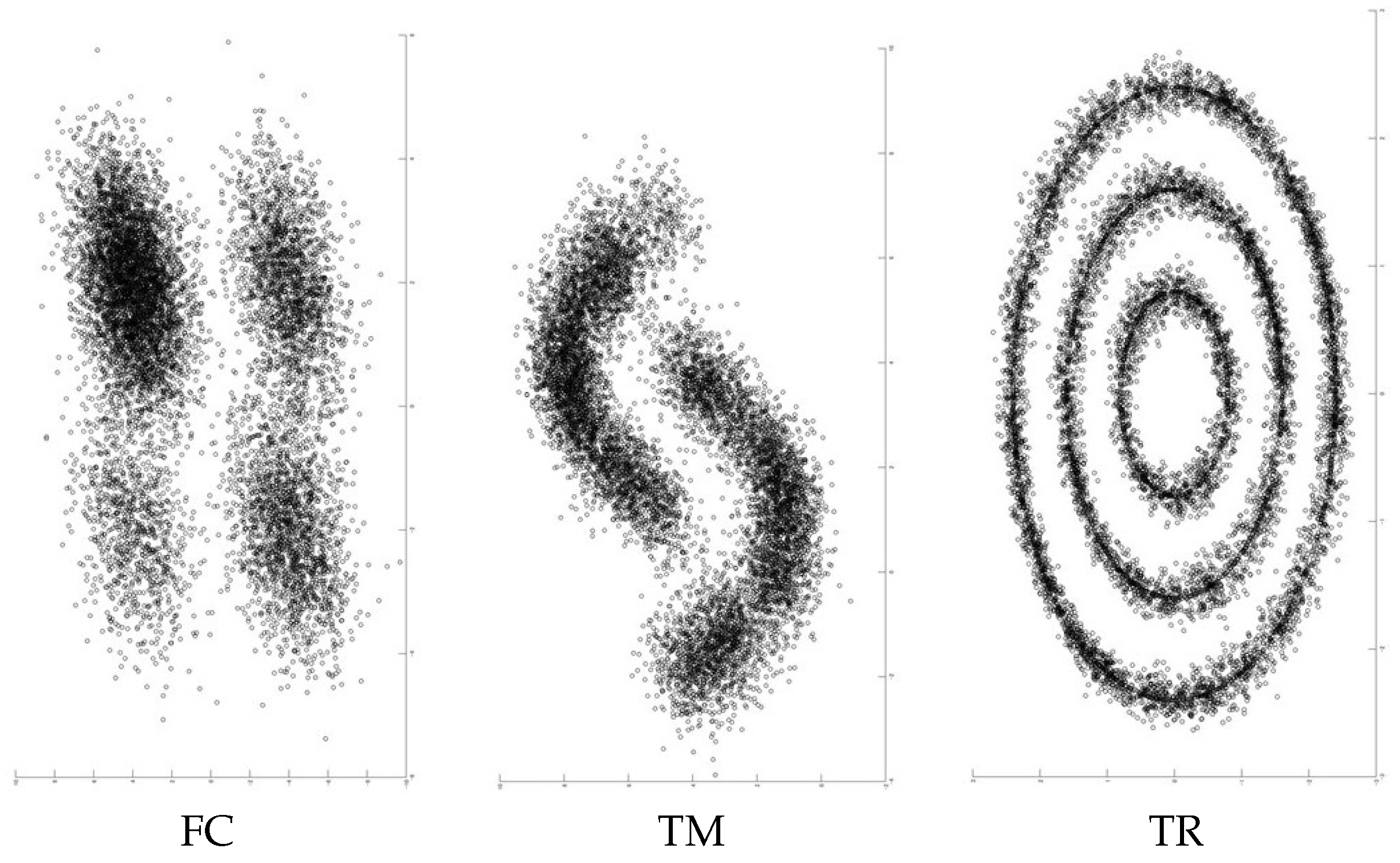
MNIST is a collection of 28 × 28 gray-scale images of handwritten digits. It is composed of 60,000 training and 10,000 test sets. The digits are transformed to 784-dimensional feature vectors. Then, they are centered, and the size is normalized. In this experiment, we use all 70,000 data points. Reuters-10k is a dataset of English news stories labeled with a category tree [42]. Following [12], we used the same four root labels. The news stories are transformed to feature vectors by computing the TF-IDF features on the 2000 most frequent words. This dataset contains 685,071 documents. In this experiment, random subsets of 10,000 samples from the full dataset are drawn. As for the synthetic datasets, we show the generated examples in Figure 2. An example of FC is the left picture in the figure. This dataset is composed of simple four clusters with some outliers. The cluster balance is biased. The ratio of biggest cluster is to the dataset, then and . The four clusters are close to each other. An example of TM is middle picture in the table. This dataset includes some outliers and its decision boundary is non-linear. The cluster balance is uniform. The example of TR is the right picture in Table Figure 2. This dataset is composed of three concentric rings. The ratio of outer ring to the whole size is , and the middle and inner ones are and , respectively.
Regarding the evaluation metric, since we are in unsupervised learning scenario, we adopt the standard metric for evaluating clustering performance [12,15], which measures how close the estimated cluster labels are to the ground truth. For an unlabeled dataset , let and be its true cluster label set and estimated cluster label set, respectively. The number of data points is denoted by n. Suppose that the both true and estimated cluster labels and take the same range, i.e., . The clustering accuracy (ACC) is then defined by
where ranges over all permutations of cluster labels, and is the indicator function given by
The optimal assignment of can be computed using the Kuhn–Munkres algorithm [43].
4.2. Performance Evaluation of SGSC
We here show how accurately SGSC could estimate the cluster labels of five datasets in Table 3. Strictly speaking, SGSC of Algorithm 1 has five hyperparameters, which are , of Equation (1), , h and . In this experiment, we nevertheless do not consider and as the hyperparameters. The reason is, when median heuristics and were employed to and respectively, SGSC performed well throughout all datasets of Table 3 in our preliminary experiments. Thus, we consider the rest three as the hyperparameters.
Generally speaking, in unsupervised learning, it is difficult to tune hyperparameters because we cannot conduct cross-validation. However, by using the idea of transfer learning, we can ease the difficulty. Following [15], we tune the three aforementioned hyperparameters. Let be the triplet . The best one is denoted by . Now, is defined as follows:
where is i-th source domain. is the best hyperparameter for the . is the clustering accuracy of Equation (9) when the hyperparameter is selected for . The dataset on which we want to compute the clusters will be referred to as target domain. The source domain of each given dataset is shown in Table 4. USPS [44] is a dataset of handwritten digit. The number of clusters is ten. 20news [15] is a dataset of newsgroup documents, which is partitioned nearly evenly across 20 different newsgroups. The source domain of FC is FC, TM, and TR. Please note that FC, TM, and TR used as sources have slightly different generating rules compared to target ones. The same things goes for the target TM and TR datasets. By using these source domains, we tune the hyperparameters.
As for the ranges of candidates with three hyperparameters, we define , and . By conducting tuning technique of Equation (11) on each source domain, we obtained the best hyperparameters for given datasets of Table 3 as follows: The best ones for MNIST, Reuters-10k, FC, TM, and TR are , , , and respectively. For an example, when , we obtained the accuracy matrix for both MNIST and USPS shown in Table 5. According to this table, the best pair of USPS is transferred to MNIST. Finally, based on the above best pair of hyperparameters, we conduct SGSC on each target dataset. The results are shown in Table 6.
4.3. Performance Evaluation of SEDC
We here show how accurately SEDC can cluster the five given datasets of Table 3, and how to proceed in implementing it. Across all the datasets, we define the network structure of by D-1200-1200-C, where D and C are the dimension of feature vector and the number of clusters, respectively. We used ReLU [45] for all the activation functions, and employed batch normalization technique [46] on each layer. For the Adam optimizer, we set the learning rate to 0.002. Following [47], we initialized the bias term and the weights of directed edges in the deep neural network as follows: each weight is initialized by the value of a Gaussian distribution with a mean of 0, and standard deviation of , where is the number of input neurons. We set the to -- for weight matrices from the input to the output. The all bias terms were initialized to 0. The number of epochs is fixed to 25, and each epoch is made by 100 iterations. As for the mini-batch with Equation (8), in each iteration, we sample and data points from the pseudo labeled dataset and the unlabeled dataset, respectively. The pseudo labeled samples are used for approximating the second term of Equation (8), and both pseudo labeled and unlabeled samples are used for approximating the first and third terms of Equation (8). Moreover, in VAT, we set to ten in Equation (5). The radius is defined by the same way as [15]: see Remark 1.
With respect to the selection of hyperparameters in SEDC, since we have already finished to tune and h in the previous section, we only focus on the remaining hyperparameters and . The tuning tactic is also based on Equation (11), and the source domains of Table 4 are used for the tuning. The ranges of candidates are defined by as follows: , . After the tuning, we obtained as the best ones for all datasets. By using the tuned hyperparameters and computing the SEDC, we get the results shown in Table 7.
As we can see in Table 7, our method averagely performs better than other methods. One of the reason is that we do not require key conditions to SEDC. For an example, IMSAT does not perform well for datasets with non-uniform cluster balance such as TR. In addition to the wide applicability, another reason lies on the robustness against outliers. When we see the performance of SEDC on FC which includes outliers, the method is more robust against outliers compared to SpectralNet. In fact, SpectralNet suffered from the two datasets which include outliers. Please note that the hyperparameter tuning of SEDC hugely contributes to the robustness. On the other hand, if we see some columns of Table 7 such as MNIST and Reuters-10k, SEDC does not outperform IMSAT. The clustering accuracy of IMSAT with MNIST is known to be one of the best results among several deep clustering methods [48]. In addition to VAT regularization, the almost perfect prior knowledge of cluster balance with MNIST seems to greatly help IMSAT achieve such the result. Though our method employs similar objective function with IMSAT, since we use the estimated cluster labels, the estimation error degraded the performance of SEDC. As for Reuters-10k, we can list two reasons why SEDC does not outperform IMSAT well. The first one is that the number of given data points is not enough since the geodesic metric is approximated by the graph shortest path distance in SEDC. In fact, we observed that by using 20,000 unlabeled data points with Reuters, the clustering accuracy of SEDC and IMSAT were 0.739 (0.06) and 0.696 (0.05), respectively. The accuracy was the average of seven times experiments. The second one is that the source domain of Reuters-10k might be not appropriate since the cluster balances of 20new and Reuters are uniform and non-uniform, respectively.
In Table 8, we show the corresponding mean runtime and standard deviation of Table 7. As we can expect, k-means is the fastest clustering method among the six. The runtime of SC is quite long especially when the size of dataset is large. The most heavy computation is in solving the eigenvalue problem. IMSAT is the second slowest method in the six. Since this method require the k-NN graph for defining the adaptive radius with VAT: see Remark 1, this computation is dominant in the whole procedure. In addition to the time of graph construction, relatively larger number of epochs (50 epochs) for training the deep neural network also affected the total runtime. DEC is the fastest method among the deep clustering methods. After the pre-training, DEC simply trains the deep neural network by using mini-batches until the convergence. Please note that the shown runtimes of DEC do not include the runtimes consumed on the pre-training. If we combine the runtime of that pre-training with shown ones, the total runtimes of DEC will be much longer: see Section 4.3 of [12]. SpectralNet also computes k-NN graph. Therefore, the dominant part of computation is the graph construction. In addition to this constructing time, since the number of epochs for training the two deep neural networks are not large, the total runtime of SpectralNet is relatively fast among the four deep clustering methods. Regarding with SEDC, as we already mentioned in Section 3.3, the dominant part is computing k-NN graph. In addition to this computing, since we set 25 epochs to the training, the total runtimes is medium.
5. Conclusions and Future Work
In this paper, we propose a deep clustering method named SEDC. Given an unlabeled dataset and the number of clusters, the method groups the dataset into the given number clusters. Regarding its advantages, it does not require an additional condition except two fundamental assumptions: smoothness and manifolds assumptions. In this point, only SpectralNet of Table 1 is comparable. In addition, SEDC also can be applied to various data domains since it does not have preferred data domains, as long as raw data is transformed to feature vectors. Furthermore, the performance of SEDC can be robust against existence of outliers unlike SpectralNet. According to these advantages, our proposed method can be expected to averagely perform better than previous deep clustering methods. As a result, this expectation is empirically confirmed by conducting numerical experiments on five commonly used datasets: see Table 7. Therefore, we think our method can be a competitive candidate for users in some practical clustering scenarios where prior knowledge of the given unlabeled dataset is limited.
However, there are two main drawbacks. On the one hand, since the method needs hyperparameter tuning, if we do not have appropriate labeled source domains to learn them from and transfer, then it may fail. On the other hand, since the method requires the number of clusters, it does not work for datasets where nothing is known on the number of clusters such as genome datasets.
Finally, we discuss about our two future works. The first one is to invent a more noise-robust semi-supervised learning framework and then apply it to SEDC instead of Equation (8). Since some of the estimated cluster labels by SGSC are not perfectly accurate, we need to invent such the framework to stabilize the performance of SEDC. The second one is to modify our method for handling structured data, i.e., graph data or sequential data.
Author Contributions
Conceptualization, Y.W., T.N., L.A., W.K., and T.K.; Methodology, Y.W., L.A., W.K., and T.K.; Software, Y.W., S.M., T.N., and L.A.; Validation, Y.W., S.M., T.N., L.A., W.K., and T.K.; Formal Analysis, Y.W., L.A., W.K., and T.K.; Investigation, Y.W., S.M., T.N., L.A., W.K., and T.K.; Resources, Y.W., S.M., T.N., and L.A.; Data Curation, Y.W., S.M., T.N., and L.A.; Writing―Original Draft Preparation, Y.W., L.A., W.K., and T.K.; Writing―Review & Editing, Y.W., L.A., W.K., and T.K.; Visualization, Y.W., and L.A.; Supervision, T.K.; Project Administration, Y.W. and T.K.; Funding Acquisition, W.K., and T.K.
Funding
WK was partially supported by JSPS KAKENHI Grant Number 17K12653. TK was partially supported by JSPS KAKENHI Grant Number15H01678, 15H03636, 16K00044, and 19H04071.
Acknowledgments
We would deeply like to thank the members of Takafumi Kanamori laboratory in Tokyo Institute of Technology, the members of Masahiko Sakai laboratory in Nagoya University and all the secretaries for the progressive discussion and much support.
Conflicts of Interest
The authors declare no conflict of interest.
References
- Berkhin, P. A survey of clustering data mining techniques. In Grouping Multidimensional Data; Springer: Berlin/Heidelberg, Germany, 2006; pp. 25–71. [Google Scholar]
- Xu, R.; Wunsch, D.C. Survey of clustering algorithms. IEEE Trans. Neural Netw. 2005, 16, 645–678. [Google Scholar] [CrossRef] [PubMed]
- MacQueen, J. Some methods for classification and analysis of multivariate observations. In Proceedings of the Fifth Berkeley Symposium on Mathematical Statistics and Probability, Oakland, CA, USA, 21 June–18 July 1965 and 27 December 1965–7 January 1966; Volume 1, pp. 281–297. [Google Scholar]
- Day, N.E. Estimating the components of a mixture of normal distributions. Biometrika 1969, 56, 463–474. [Google Scholar] [CrossRef]
- Girolami, M. Mercer kernel-based clustering in feature space. IEEE Trans. Neural Netw. 2002, 13, 780–784. [Google Scholar] [CrossRef] [PubMed]
- Wang, J.; Lee, J.; Zhang, C. Kernel trick embedded Gaussian mixture model. In Proceedings of the International Conference on Algorithmic Learning Theory, Sapporo, Japan, 17–19 October 2003; pp. 159–174. [Google Scholar]
- Ng, A.Y.; Jordan, M.I.; Weiss, Y. On spectral clustering: Analysis and an algorithm. In Advances in Neural Information Processing Systems, Proceedings of the Neural Information Processing Systems, NIPS 2002, Vancouver, BC, Canada, 9–14 December 2002; MIT Press: Cambridge, MA, USA, 2002; pp. 849–856. [Google Scholar]
- Jain, A.K. Data clustering: 50 years beyond K-means. Pattern Recognit. Lett. 2010, 31, 651–666. [Google Scholar] [CrossRef]
- LeCun, Y.; Bengio, Y.; Hinton, G. Deep learning. Nature 2015, 521, 436–444. [Google Scholar] [CrossRef] [PubMed]
- Hinton, G.E.; Salakhutdinov, R.R. Reducing the dimensionality of data with neural networks. Science 2006, 313, 504–507. [Google Scholar] [CrossRef]
- Krizhevsky, A.; Sutskever, I.; Hinton, G.E. Imagenet classification with deep convolutional neural networks. In Advances in Neural Information Processing Systems, Proceedings of the NIPS 2012: Neural Information Processing Systems Conference, Lake Tahoe, NV, USA, 3–6 December 2012; MIT Press: Cambridge, MA, USA, 2012; pp. 1097–1105. [Google Scholar]
- Xie, J.; Girshick, R.; Farhadi, A. Unsupervised deep embedding for clustering analysis. In Proceedings of the International Conference on Machine Learning, New York, NY, USA, 19–24 June 2016; pp. 478–487. [Google Scholar]
- Yang, J.; Parikh, D.; Batra, D. Joint unsupervised learning of deep representations and image clusters. In Proceedings of the IEEE Conference on Computer Vision and Pattern Recognition, Las Vegas, NV, USA, 27–30 June 2016; pp. 5147–5156. [Google Scholar]
- Jiang, Z.; Zheng, Y.; Tan, H.; Tang, B.; Zhou, H. Variational deep embedding: An unsupervised and generative approach to clustering. arXiv 2016, arXiv:1611.05148. [Google Scholar]
- Hu, W.; Miyato, T.; Tokui, S.; Matsumoto, E.; Sugiyama, M. Learning Discrete Representations via Information Maximizing Self-Augmented Training. In Proceedings of the International Conference on Machine Learning, Sydney, Australia, 6–11 August 2017; pp. 1558–1567. [Google Scholar]
- Springenberg, J.T. Unsupervised and semi-supervised learning with categorical generative adversarial networks. arXiv 2015, arXiv:1511.06390. [Google Scholar]
- Shaham, U.; Stanton, K.; Li, H.; Nadler, B.; Basri, R.; Kluger, Y. SpectralNet: Spectral Clustering using Deep Neural Networks. arXiv 2018, arXiv:1801.01587. [Google Scholar]
- Chapelle, O.; Zien, A. Semi-Supervised Classification by Low Density Separation. In Proceedings of the AISTATS, Bridgetown, Barbados, 6–8 January 2005; pp. 57–64. [Google Scholar]
- Tian, F.; Gao, B.; Cui, Q.; Chen, E.; Liu, T.Y. Learning deep representations for graph clustering. In Proceedings of the Twenty-Eighth AAAI Conference on Artificial Intelligence, Québec City, QC, Canada, 27–31 July 2014. [Google Scholar]
- Huang, P.; Huang, Y.; Wang, W.; Wang, L. Deep embedding network for clustering. In Proceedings of the 2014 22nd International Conference on Pattern Recognition, Stockholm, Sweden, 24–28 August 2014; pp. 1532–1537. [Google Scholar]
- Kingma, D.P.; Welling, M. Auto-encoding variational bayes. arXiv 2013, arXiv:1312.6114. [Google Scholar]
- Shaham, U.; Lederman, R.R. Learning by coincidence: Siamese networks and common variable learning. Pattern Recognit. 2018, 74, 52–63. [Google Scholar] [CrossRef]
- Von Luxburg, U. A tutorial on spectral clustering. Stat. Comput. 2007, 17, 395–416. [Google Scholar] [CrossRef]
- Scholkopf, B.; Smola, A.J. Learning with Kernels: Support Vector Machines, Regularization, Optimization, and Beyond; MIT Press: Cambridge, MA, USA, 2001. [Google Scholar]
- Arthur, D.; Vassilvitskii, S. k-means++: The advantages of careful seeding. In Proceedings of the Eighteenth Annual ACM-SIAM Symposium on Discrete Algorithms, New Orleans, LA, 7–9 January 2007; pp. 1027–1035. [Google Scholar]
- Miyato, T.; Maeda, S.i.; Ishii, S.; Koyama, M. Virtual adversarial training: A regularization method for supervised and semi-supervised learning. IEEE Trans. Pattern Anal. Mach. Intell. 2018, 41, 1979–1993. [Google Scholar] [CrossRef] [PubMed]
- Bachman, P.; Alsharif, O.; Precup, D. Learning with pseudo-ensembles. In Advances in Neural Information Processing Systems, Proceedings of the NIPS 2014: Neural Information Processing Systems Conference, Montreal, QC, Canada, 8–13 December 2014; MIT Press: Cambridge, MA, USA, 2014; pp. 3365–3373. [Google Scholar]
- Goodfellow, I.J.; Shlens, J.; Szegedy, C. Explaining and harnessing adversarial examples. arXiv 2014, arXiv:1412.6572. [Google Scholar]
- Tao, Y.; Takagi, K.; Nakata, K. RDEC: Integrating Regularization into Deep Embedded Clustering for Imbalanced Datasets. In Proceedings of the Asian Conference on Machine Learning, Beijing, China, 14–16 November 2018; pp. 49–64. [Google Scholar]
- Cover, T.M.; Thomas, J.A. Elements of Information Theory; John Wiley & Sons: Hoboken, NJ, USA, 2012. [Google Scholar]
- Dasgupta, S.; Kpotufe, S. Optimal rates for k-NN density and mode estimation. In Advances in Neural Information Processing Systems, Proceedings of the NIPS 2014: Neural Information Processing Systems Conference, Montreal, QC, Canada, 8–13 December 2014; MIT Press: Cambridge, MA, USA, 2014; pp. 2555–2563. [Google Scholar]
- Moscovich, A.; Jaffe, A.; Nadler, B. Minimax-optimal semi-supervised regression on unknown manifolds. arXiv 2016, arXiv:1611.02221. [Google Scholar]
- Har-Peled, S. Computing the k Nearest-Neighbors for all Vertices via Dijkstra. arXiv 2016, arXiv:1607.07818. [Google Scholar]
- Maaten, L.v.d.; Hinton, G. Visualizing data using t-SNE. J. Mach. Learn. Res. 2008, 9, 2579–2605. [Google Scholar]
- Kingma, D.P.; Ba, J. Adam: A method for stochastic optimization. arXiv 2014, arXiv:1412.6980. [Google Scholar]
- Grandvalet, Y.; Bengio, Y. Semi-supervised learning by entropy minimization. In Advances in Neural Information Processing Systems, Proceedings of the 19th Annual Conference on Neural Information Processing Systems, Vancouver, BC, Canada, 5–8 December 2005; MIT Press: Cambridge, MA, USA, 2005; pp. 529–536. [Google Scholar]
- Krause, A.; Perona, P.; Gomes, R.G. Discriminative clustering by regularized information maximization. In Advances in Neural Information Processing Systems, Proceedings of the 24th Annual Conference on Neural Information Processing Systems, Vancouver, BC, Canada, 6–9 December 2010; MIT Press: Cambridge, MA, USA, 2010; pp. 775–783. [Google Scholar]
- Dong, W.; Moses, C.; Li, K. Efficient k-nearest neighbor graph construction for generic similarity measures. In Proceedings of the 20th International Conference on World Wide Web, Hyderabad, India, 28 March–1 April 2011; pp. 577–586. [Google Scholar]
- Wang, D.; Shi, L.; Cao, J. Fast algorithm for approximate k-nearest neighbor graph construction. In Proceedings of the 2013 IEEE 13th International Conference on Data Mining Workshops, Dallas, TX, USA, 7–10 December 2013; pp. 349–356. [Google Scholar]
- Zhang, Y.M.; Huang, K.; Geng, G.; Liu, C.L. Fast kNN graph construction with locality sensitive hashing. In Proceedings of the Joint European Conference on Machine Learning and Knowledge Discovery in Databases, Prague, Czech Republic, 23–27 September 2013; pp. 660–674. [Google Scholar]
- LeCun, Y.; Bottou, L.; Bengio, Y.; Haffner, P. Gradient-based learning applied to document recognition. Proc. IEEE 1998, 86, 2278–2324. [Google Scholar] [CrossRef] [Green Version]
- Lewis, D.D.; Yang, Y.; Rose, T.G.; Li, F. Rcv1: A new benchmark collection for text categorization research. J. Mach. Learn. Res. 2004, 5, 361–397. [Google Scholar]
- Kuhn, H.W. The Hungarian method for the assignment problem. Nav. Res. Logist. Q. 1955, 2, 83–97. [Google Scholar] [CrossRef] [Green Version]
- Hastie, T.; Tibshirani, R.; Friedman, J. The Elements of Statistical Learning; Springer: New York, NY, USA, 2008. [Google Scholar]
- Nair, V.; Hinton, G.E. Rectified linear units improve restricted boltzmann machines. In Proceedings of the 27th International Conference on Machine Learning (ICML-10), Haifa, Israel, 21–24 June 2010; pp. 807–814. [Google Scholar]
- Ioffe, S.; Szegedy, C. Batch normalization: Accelerating deep network training by reducing internal covariate shift. arXiv 2015, arXiv:1502.03167. [Google Scholar]
- He, K.; Zhang, X.; Ren, S.; Sun, J. Delving deep into rectifiers: Surpassing human-level performance on imagenet classification. In Proceedings of the IEEE International Conference on Computer Vision, Santiago, Chile, 7–13 December 2015; pp. 1026–1034. [Google Scholar]
- Min, E.; Guo, X.; Liu, Q.; Zhang, G.; Cui, J.; Long, J. A survey of clustering with deep learning: From the perspective of network architecture. IEEE Access 2018, 6, 39501–39514. [Google Scholar] [CrossRef]
Figure 1.
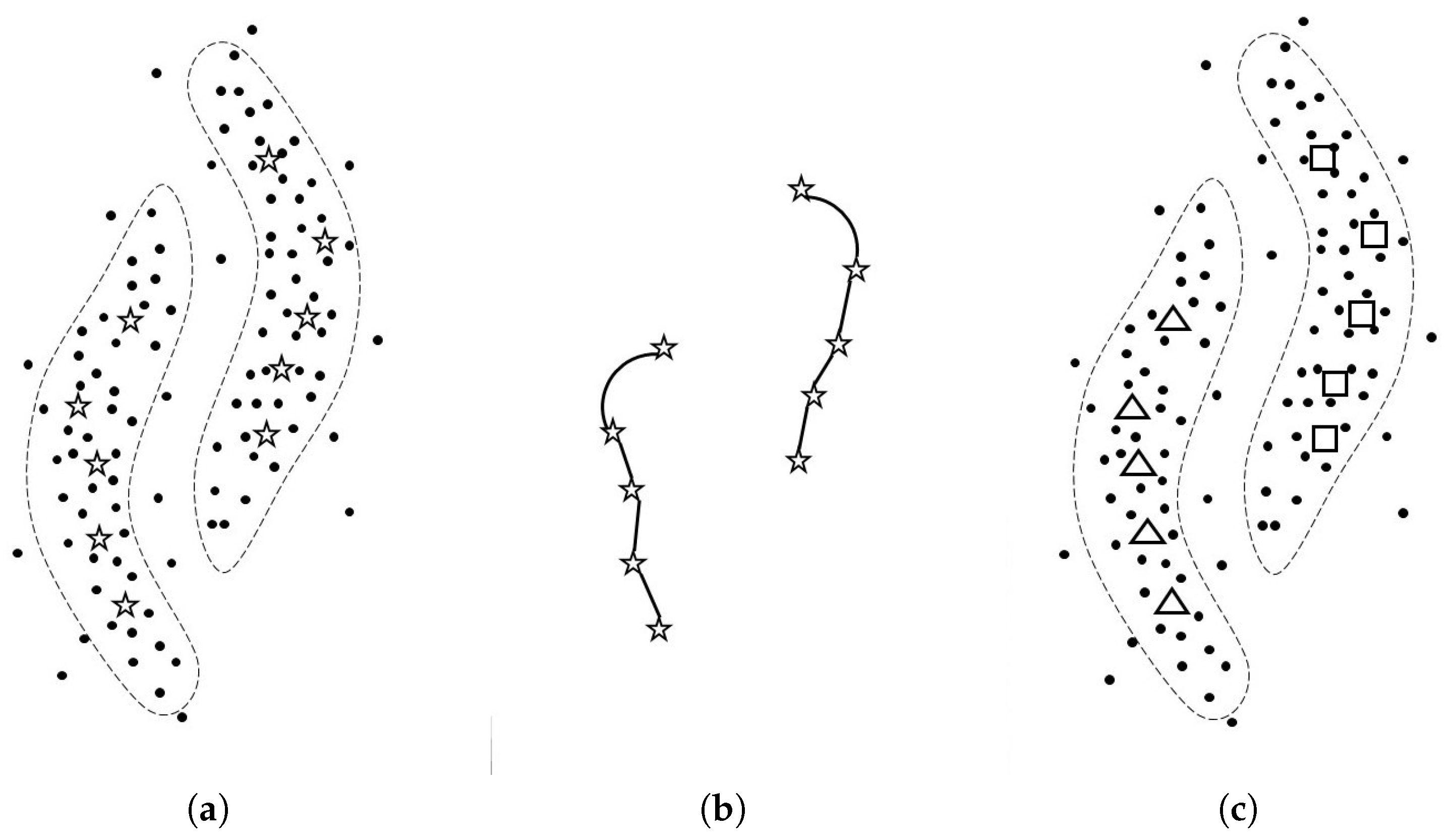
This figure explains how SGSC works. (a): Given unlabeled data points, in line 2 of Algorithm 1, SGSC computes the hub data points. The hub data points are expressed by star symbols, and the number of hub data points h is ten in this case; (b): In line 4 of the algorithm, SGSC focuses only on the hub data points, then conducts SC with the geodesic metric on those hub points, where we set one to ; (c): As the results, we obtain the cluster labels of hub points. The triangle and square symbols mean different labels. Please note that an actual output of SGSC is the estimated conditional discrete probability distributions with hub data points, but we can obtain the estimated cluster labels from the distributions.
Figure 1.
This figure explains how SGSC works. (a): Given unlabeled data points, in line 2 of Algorithm 1, SGSC computes the hub data points. The hub data points are expressed by star symbols, and the number of hub data points h is ten in this case; (b): In line 4 of the algorithm, SGSC focuses only on the hub data points, then conducts SC with the geodesic metric on those hub points, where we set one to ; (c): As the results, we obtain the cluster labels of hub points. The triangle and square symbols mean different labels. Please note that an actual output of SGSC is the estimated conditional discrete probability distributions with hub data points, but we can obtain the estimated cluster labels from the distributions.

Figure 2.
The generated examples of three commonly used synthetic datasets. The left, middle and right pictures correspond the examples of four clusters (FC), two moons (TM) and three rings (TR), respectively.
Figure 2.
The generated examples of three commonly used synthetic datasets. The left, middle and right pictures correspond the examples of four clusters (FC), two moons (TM) and three rings (TR), respectively.


Table 1.
Summary of popular deep clustering methods. Three AE-based methods and four direct methods are presented, including our method SEDC. A method has a preferred domain when it is specialized for a certain type of data. Please note that all methods require the smoothness and manifold assumptions. Some methods require additional key conditions except the above two assumptions. Empty spaces mean “None”. All methods below require the number of clusters as one of their inputs.
| AE-Based Methods | Preferred Domain | Key Condition |
|---|---|---|
| DEC [12] | AE acquires good representation. | |
| JULE [13] | Image | Size of dataset is not large. |
| VaDE [14] | The representation follows GMM. | |
| Direct Methods | Preferred Domain | Key Condition |
| IMSAT [15] | Cluster balance is uniform. | |
| CatGAN [16] | Cluster balance is uniform. | |
| SpectralNet [17] | ||
| SEDC |
Table 2.
The computational complexity of each line of Algorithm 1 (SGSC algorithm), where and are the dimension of the feature vector, the number of given unlabeled data points, the number of hub data points and the number of neighbors, respectively.
Table 2.
The computational complexity of each line of Algorithm 1 (SGSC algorithm), where and are the dimension of the feature vector, the number of given unlabeled data points, the number of hub data points and the number of neighbors, respectively.
| Corresponding Line of Algorithm 1 | Line 1 | Line 2 | Line 3 | Line 4 |
|---|---|---|---|---|
| Theoretical computational complexity |
Table 3.
Summary of dataset statistics. #Points is the number of data points used for the training of each clustering method. #Clusters is the given number of clusters. Dimension is the dimension of given feature vector. %Largest cluster means the percentage of the largest cluster size to each size of dataset.
| Dataset | #Points | #Clusters | Dimension | %Largest cluster |
|---|---|---|---|---|
| MNIST | 70,000 | 10 | 784 | 11% |
| Reuters-10k | 10,000 | 4 | 2000 | 43% |
| FC | 10,000 | 4 | 2 | 50% |
| TM | 10,000 | 2 | 2 | 50% |
| TR | 10,000 | 3 | 2 | 50% |
Table 4.
The source domain is a dataset we can use to tune our hyperparameters. Dimension means the dimension of feature vector with source dataset. #Points means the number of data points with source dataset. The target domain is a dataset which we want to cluster using knowledge from the source.
Table 4.
The source domain is a dataset we can use to tune our hyperparameters. Dimension means the dimension of feature vector with source dataset. #Points means the number of data points with source dataset. The target domain is a dataset which we want to cluster using knowledge from the source.
| Source Domain | Dimension | #Points | Target Domain |
|---|---|---|---|
| USPS | 256 | MNIST | |
| 20news | 2000 | Reuters-10k | |
| (FC, TM, TR) | (2, 2, 2) | (, , ) | FC |
| (FC, TM, TR) | (2, 2, 2) | (, , ) | TM |
| (FC, TM, TR) | (2, 2, 2) | (, , ) | TR |
Table 5.
The accuracy of estimated labels with hub data points for both MNIST and USPS is shown. The labels are estimated by SGSC. and h mean the number of neighbors and the number of hub data points, respectively. Each accuracy is computed by the output of SGSC using corresponding the pair . Another number of neighbors used in the SGSC is fixed to ten. The bold font below means the best accuracy for each dataset. Please note that since we use all data points of both MNIST and USPS for the estimation, no standard deviation is shown.
| Dataset | 5 | 10 | 15 | 20 | 25 | ||
|---|---|---|---|---|---|---|---|
| h | |||||||
| Target: | 200 | 0.88 | 0.78 | 0.76 | 0.75 | 0.79 | |
| 300 | 0.45 | 0.92 | 0.91 | 0.90 | 0.89 | ||
| MNIST | 400 | 0.79 | 0.83 | 0.86 | 0.90 | 0.88 | |
| 500 | 0.39 | 0.88 | 0.86 | 0.86 | 0.89 | ||
| Source: | 200 | 0.59 | 0.49 | 0.51 | 0.44 | 0.46 | |
| 300 | 0.49 | 0.65 | 0.49 | 0.52 | 0.48 | ||
| USPS | 400 | 0.65 | 0.61 | 0.63 | 0.48 | 0.50 | |
| 500 | 0.68 | 0.69 | 0.64 | 0.65 | 0.53 | ||
Table 6.
The mean accuracy and standard deviation obtained by SGSC using best hyperparameters are shown. These numbers are averaged number over seven times experiments. Since we use all samples of MNIST for the estimation, no standard deviation is shown.
Table 6.
The mean accuracy and standard deviation obtained by SGSC using best hyperparameters are shown. These numbers are averaged number over seven times experiments. Since we use all samples of MNIST for the estimation, no standard deviation is shown.
| MNIST | Reuters-10k | FC | TM | TR |
|---|---|---|---|---|
| 0.88 | 0.78 (0.06) | 0.94 (0.04) | 0.98 (0.01) | 0.97 (0.02) |
Table 7.
The mean clustering accuracy (ACC) of Equation (9) and standard deviation are shown. Five popular clustering methods and our proposed method were tested on five datasets. For each method, Average means the averaged ACC over the five datasets. The experiments were conducted seven times on each pair of method and dataset. For each dataset, the bold font means the highest accuracy among six methods.
| Method | MNIST | Reuters-10k | FC | TM | TR | Average |
|---|---|---|---|---|---|---|
| k-means | 0.53 | 0.53 (0.04) | 0.60 (0.05) | 0.64 (0.04) | 0.35 (0.03) | 0.53 |
| SC | 0.72 | 0.62 (0.03) | 0.80 (0.04) | 0.85 (0.03) | 0.96 (0.03) | 0.79 |
| IMSAT | 0.98 | 0.71 (0.05) | 0.70 (0.04) | 0.66 (0.05) | 0.34 (0.01) | 0.68 |
| DEC | 0.84 | 0.72 (0.05) | 0.72 (0.04) | 0.67 (0.03) | 0.48 (0.04) | 0.69 |
| SpectralNet | 0.83 | 0.67 (0.03) | 0.79 (0.03) | 0.87 (0.02) | 0.99 (0.01) | 0.83 |
| SEDC | 0.89 | 0.73 (0.05) | 0.95 (0.03) | 0.96 (0.02) | 0.99 (0.00) | 0.90 |
Table 8.
The corresponding mean runtime (seconds) and standard deviation of Table 7 are shown. Five popular clustering methods and our proposed method were tested on five datasets. For each method, Average means the averaged runtimes over the five datasets. The experiments were conducted seven times on each pair of method and dataset. Please note that the runtimes of SC, IMSAT, SpectralNet, and SEDC do not include the runtimes of hyperparameter tuning. As for DEC, the runtime does not include the runtime of pre-training. The bold font means the fastest runtime among six methods.
| Method | MNIST | Reuters-10k | FC | TM | TR | Average |
|---|---|---|---|---|---|---|
| k-means | 136 | 30 (2.3) | 0.04 (0.0) | 0.05 (0.0) | 0.03 (0.0) | 33.2 |
| SC | 96,362 | 473 (5.7) | 417 (4.3) | 408 (5.1) | 413 (4.9) | 19,614 |
| IMSAT | 5097 | 749 (8.2) | 429 (5.0) | 424 (4.7) | 428 (3.8) | 1425 |
| DEC | 1274 | 258 (3.1) | 121 (4.9) | 135 (5.2) | 153 (6.6) | 388 |
| SpectralNet | 2239 | 232 (2.4) | 122 (2.0) | 110 (2.3) | 117 (2.5) | 564 |
| SEDC | 3466 | 440 (4.4) | 226 (1.9) | 233 (3.0) | 237 (3.4) | 920 |
© 2019 by the authors. Licensee MDPI, Basel, Switzerland. This article is an open access article distributed under the terms and conditions of the Creative Commons Attribution (CC BY) license (http://creativecommons.org/licenses/by/4.0/).
Share and Cite
MDPI and ACS Style
Wada, Y.; Miyamoto, S.; Nakagama, T.; Andéol, L.; Kumagai, W.; Kanamori, T. Spectral Embedded Deep Clustering. Entropy 2019, 21, 795. https://doi.org/10.3390/e21080795
AMA Style
Wada Y, Miyamoto S, Nakagama T, Andéol L, Kumagai W, Kanamori T. Spectral Embedded Deep Clustering. Entropy. 2019; 21(8):795. https://doi.org/10.3390/e21080795
Chicago/Turabian StyleWada, Yuichiro, Shugo Miyamoto, Takumi Nakagama, Léo Andéol, Wataru Kumagai, and Takafumi Kanamori. 2019. "Spectral Embedded Deep Clustering" Entropy 21, no. 8: 795. https://doi.org/10.3390/e21080795
Note that from the first issue of 2016, this journal uses article numbers instead of page numbers. See further details here.