Statistical Features in High-Frequency Bands of Interictal iEEG Work Efficiently in Identifying the Seizure Onset Zone in Patients with Focal Epilepsy

 ,
,  , , ,
, , ,  and
and 
Abstract
:1. Introduction
- We propose 12 feature extraction methods, consisting of nine statistical and three entropy measure features that are important to characterize epileptic signals. Several studies of epilepsy used these statistical features to characterize normal and epileptic brain activities [7,8,9,10], which provide evidence to support the use of statistical features. To the best of our knowledge, this is the first time an investigation has been carried out to detect the SOZ electrodes based on statistical methods using HFCs (ripple and fast ripple bands).
- A data-driven grid search method using MI scores is developed to optimize bands and features jointly. The joint selection of appropriate bands and features related to epileptic activities may improve the performance of the proposed computer-aided solution and this joint selection has not been reported in previous SOZ detection studies.
- We compared different designs with SVM and standard state-of-the-art LightGBM classifiers and selected an optimal method to provide a graphical representation for epileptologists to identify the possible SOZ channels. The SOZ detection was performed based on the scoring for each segment of channels estimated using the LightGBM algorithm.
2. Data and Methods
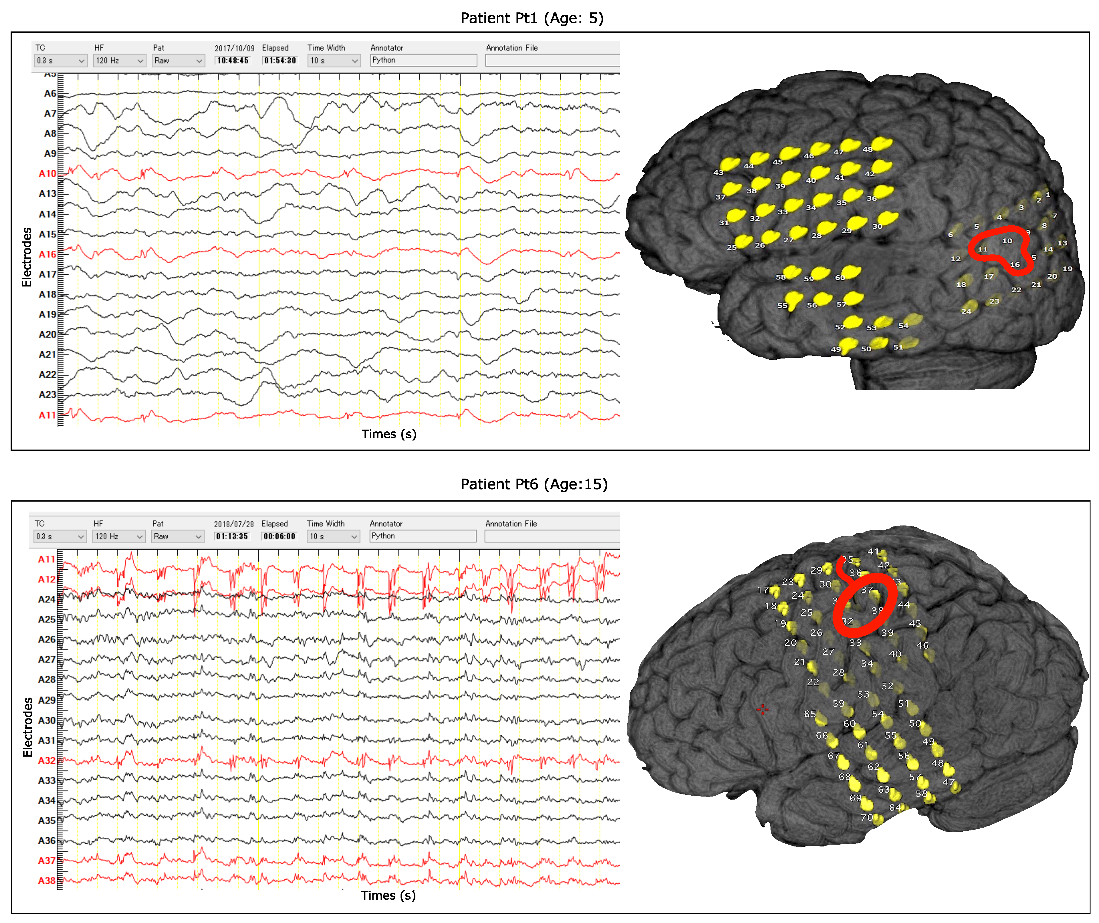
2.1. Dataset
2.2. Segmentations and Filter Bank Analysis
2.3. Feature Extraction Methods
2.3.1. Coefficient of Variation
2.3.2. Fluctuation Index
2.3.3. Variance
2.3.4. Root Mean Square
2.3.5. Difference Absolute Standard Deviation
2.3.6. Mean Absolute Value
2.3.7. Modified Mean Absolute Value
2.3.8. Modified Mean Absolute Value 2
2.3.9. Log Detector
2.3.10. Permutation Entropy
2.3.11. Spectral Entropy
2.4. Feature Concatenation
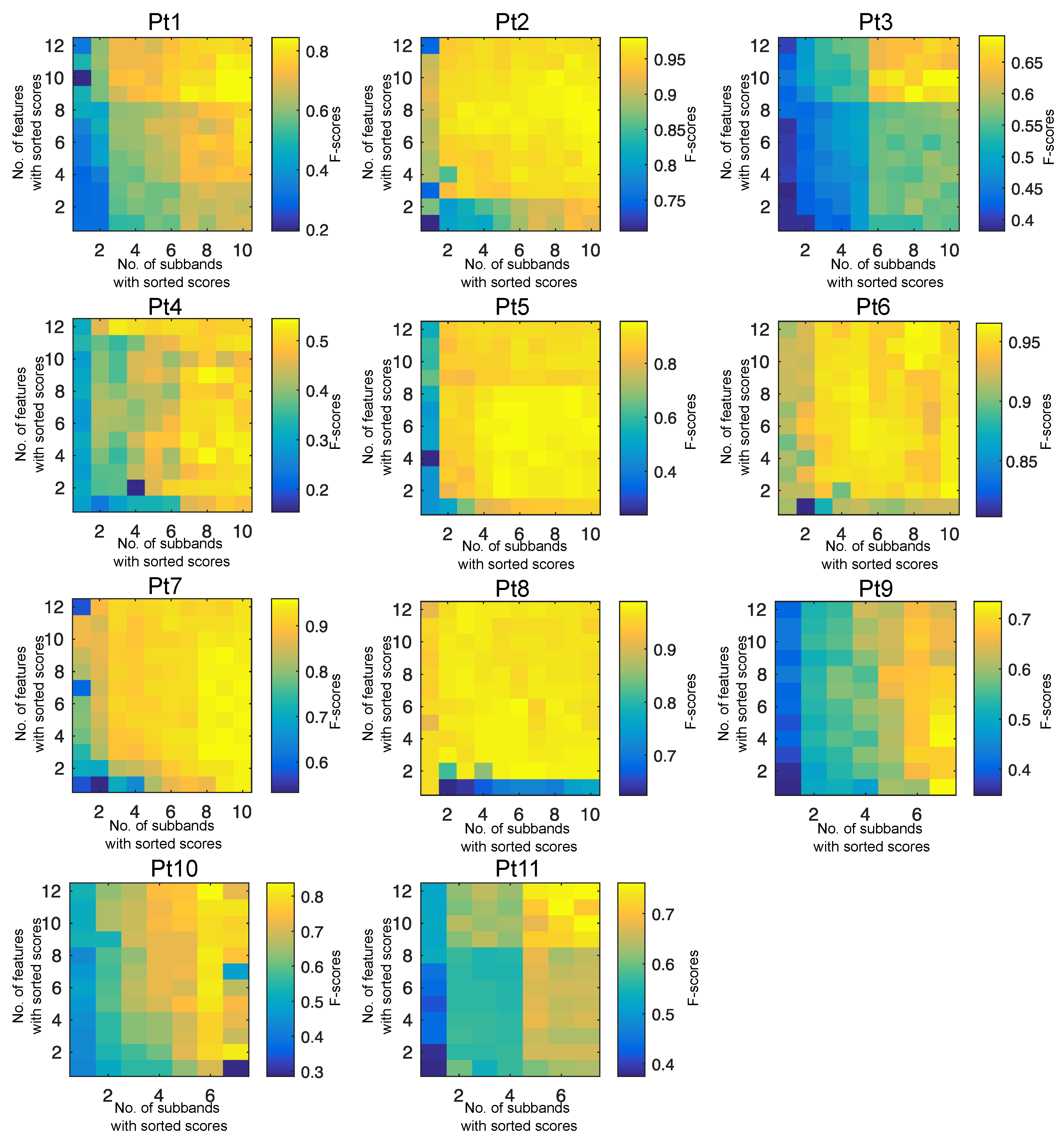
2.5. Subband and Feature Selection Method
2.5.1. Subband Scoring
2.5.2. Feature Scoring
2.6. Classifiers
2.6.1. Support Vector Machine
2.6.2. LightGBM
2.7. Evaluation
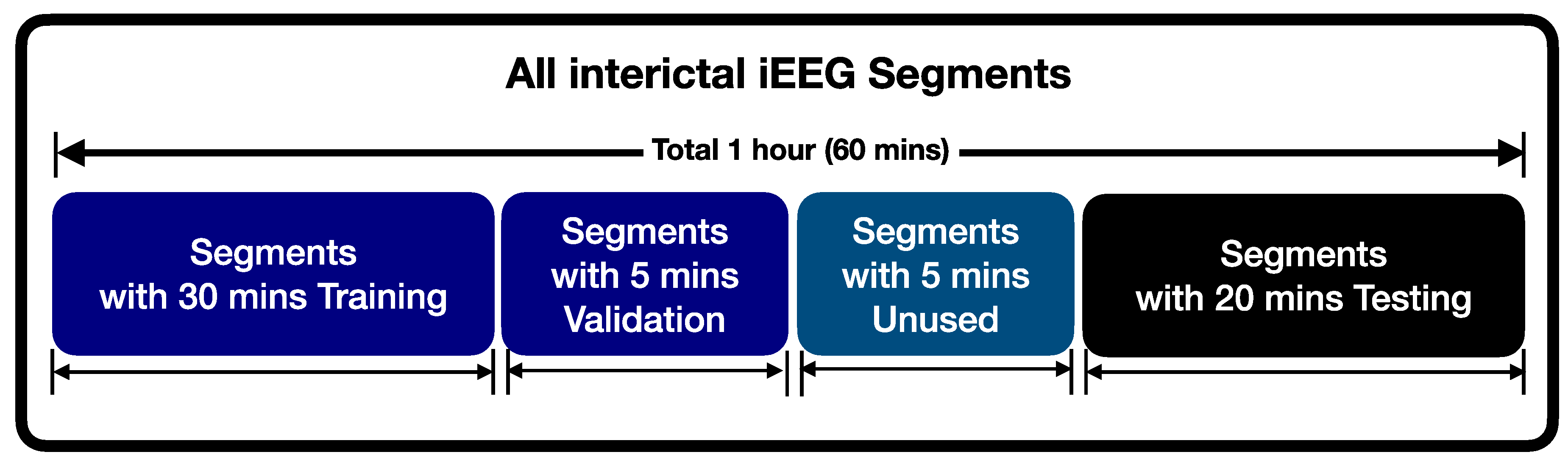
2.7.1. Division of iEEG Time Series for Training and Testing
2.7.2. Segment-Wise Performance Measurement
2.7.3. Channel-Wise Performance Measurement
3. Results
- Filter bank Feature Extraction Method (FbFM): The multi-channel interictal iEEG signals were split into 20 s segments. The N bandpass filters were implemented using a third-order Butterworth filter to decompose each segment of the high-frequency components (ripple and fast ripple) in iEEG. The different types of statistical feature extraction methods were applied to each subband to extract features. An SVM and LightGBM with the ADASYN method were used to score each electrode for identifying possible SOZ channels.
- FbFM with Subband and Feature Selection (FBFM/Sb/FS): In this case, subbanding and feature extraction were applied in the same way as the above (FbFM) method. A data-driven grid search method using scores was proposed to select both epileptic-related bands and prominent features. The ADASYN approach, SVM and LightGBM were also used to score channels.
3.1. Selection of Optimal Features and Subbands
3.2. Results for Detected Segments
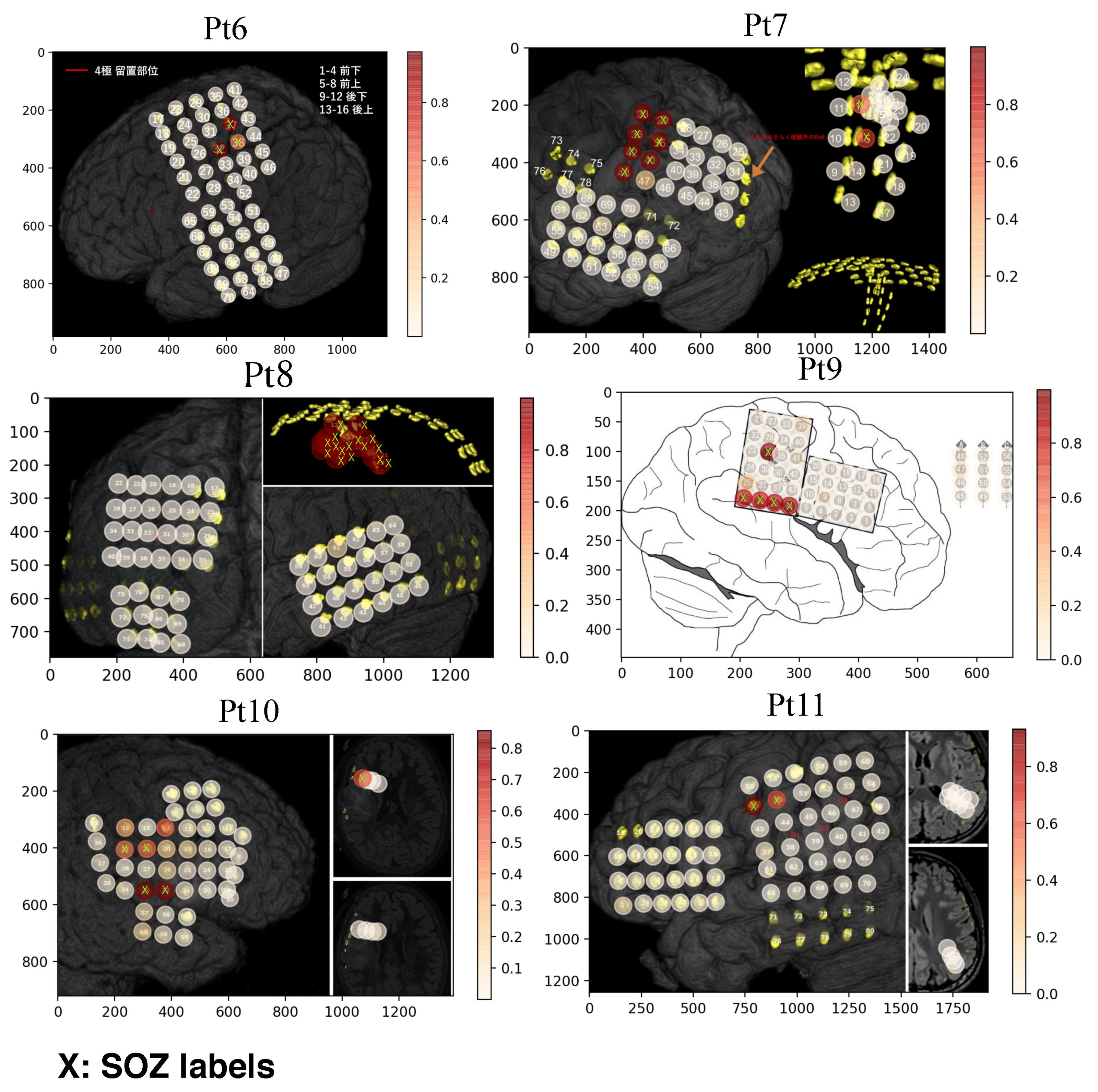
3.3. Results for Localizing SOZ channels
3.4. Comparison Between Patient-Dependent and -Independent Designs
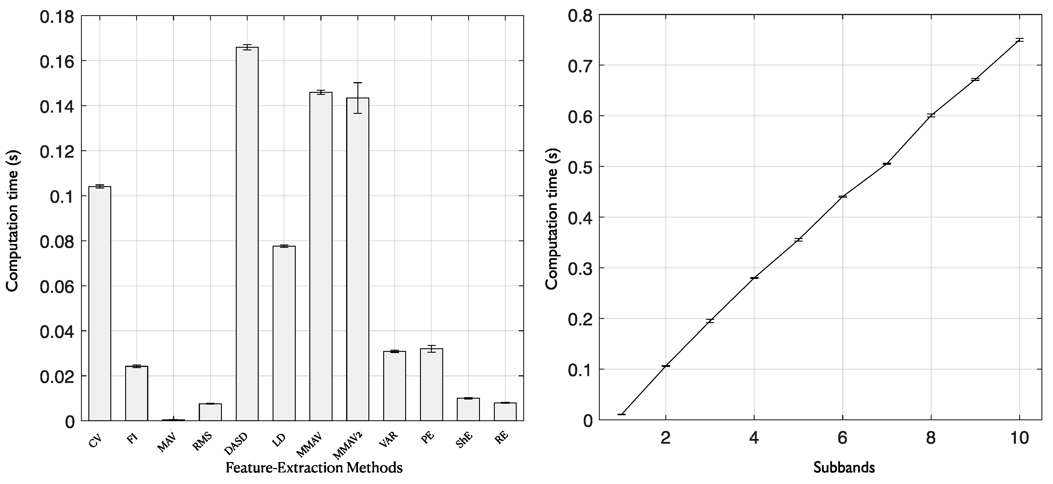
3.5. Computational Cost Analysis
4. Discussion
5. Conclusions
Author Contributions
Funding
Conflicts of Interest
References
- Fisher, R.S.; Acevedo, C.; Arzimanoglou, A.; Bogacz, A.; Cross, J.H.; Elger, C.E.; Engel, J.; Forsgren, L.; French, J.A.; Glynn, M.; et al. ILAE Official Report: A Practical Clinical Definition of Epilepsy. Epilepsia 2014, 55, 475–482. [Google Scholar] [CrossRef] [Green Version]
- Pati, S.; Alexopoulos, A. Pharmacoresistant epilepsy: From Pathogenesis to Current and Emerging Therapies. Clevel. Clin. J. Med. 2010, 77, 457–467. [Google Scholar] [CrossRef] [PubMed] [Green Version]
- Yaffe, R.B.; Borger, P.; Megevand, P.; Groppe, D.M.; Kramer, M.A.; Chu, C.J.; Santaniello, S.; Meisel, C.; Mehta, A.D.; Sarma, S.V. Physiology of Functional and Effective Networks in Epilepsy. Clin. Neurophysiol. 2015, 126, 227–236. [Google Scholar] [CrossRef] [PubMed]
- Ngugi, A.; Kariuki, S.; Bottomley, C.; Kleinschmidt, I.; Sander, J.; Newton, C. Incidence of Epilepsy. Neurology 2011, 77, 1005–1012. [Google Scholar] [CrossRef] [PubMed]
- Van Mierlo, P.; Papadopoulou, M.; Carrette, E.; Boon, P.; Vandenberghe, S.; Vonck, K.; Marinazzo, D. Functional Brain Connectivity from EEG in Epilepsy: Seizure Prediction and Epileptogenic Focus Localization. Prog. Neurobiol. 2014, 121, 19–35. [Google Scholar] [CrossRef]
- Lüders, H.O.; Najm, I.; Nair, D.; Widdess-Walsh, P.; Bingman, W. The Epileptogenic Zone: General Principles. Epileptic Disord. 2006, 8, 1–9. [Google Scholar]
- Gotman, J. Automatic Recognition of Epileptic Eeizures in the EEG. Electroencephalogr. Clin. Neurophysiol. 1982, 54, 530–540. [Google Scholar] [CrossRef]
- Khan, Y.; Gotman, J. Wavelet Based Automatic Seizure Detection in intracerebral Electroencephalogram. Clin. Neurophysiol. 2003, 114, 898–908. [Google Scholar] [CrossRef]
- Li, S.; Zhou, W.; Yuan, Q.; Geng, S.; Cai, D. Feature Extraction and Recognition of Ictal EEG using EMD and SVM. Comput. Biol. Med. 2013, 43, 807–816. [Google Scholar] [CrossRef]
- Hassan, K.M.; Islam, M.R.; Tanaka, T.; Molla, M.K.I. Epileptic Seizure Detection from EEG Signals Using Multiband Features with Feedforward Neural Network. In Proceedings of the International Conference on Cyberworlds (CW), Kyoto, Japan, 2–4 October 2019; pp. 231–238. [Google Scholar]
- Sharma, R.; Pachori, R.B.; Gautam, S. Empirical Mode Decomposition based Classification of Focal and Non-focal EEG Signals. In Proceedings of the International Conference on Medical Biometrics, Shenzhen, China, 30 May–1 June 2014; pp. 135–140. [Google Scholar]
- Sharma, R.; Pachori, R.B.; Acharya, U.R. Application of Entropy Measures on Intrinsic Mode Functions for the Automated Identification of Focal Electroencephalogram Signals. Entropy 2015, 2, 669–691. [Google Scholar] [CrossRef]
- Arunkumar, N.; Ramkumar, K.; Venkatraman, V.; Abdulhay, E.; Fernandes, S.L.; Kadry, S.; Segal, S. Classification of Focal and Non Focal EEG using Entropies. Pattern Recognit. Lett. 2017, 94, 112–117. [Google Scholar]
- Itakura, T.; Tanaka, T. Epileptic Focus Localization based on Bivariate Empirical Mode Decomposition and Entropy. In Proceedings of the Asia-Pacific Signal and Information Processing Association Annual Summit and Conference (APSIPA ASC), Kuala Lumpur, Malaysia, 12–15 December 2017; pp. 1426–1429. [Google Scholar]
- Sriraam, N.; Raghu, S. Classification of Focal and Non Focal Epileptic Seizures using Multi-features and SVM Classifier. J. Med Syst. 2017, 41, 160. [Google Scholar] [CrossRef]
- Akter, M.S.; Islam, M.R.; Iimura, Y.; Sugano, H.; Fukumori, K.; Wang, D.; Tanaka, T.; Cichocki, A. Multiband Entropy–based Feature–extraction Method for Automatic Identification of Epileptic Focus based on High-frequency Components in Interictal iEEG. Sci. Rep. 2020, 10, 1–17. [Google Scholar] [CrossRef] [PubMed]
- Akter, M.S.; Islam, M.R.; Fukumori, K.; Iimura, Y.; Sugano, H.; Tanaka, T. Automatic Detection of Epileptic Focus in Ripple and Fast Ripple Bands of Interictal iEEG based on Multi–band Analysis. In Proceedings of the International Conference on Artificial Intelligence in Information and Communication (ICAIIC), Fukuoka, Japan, 19–21 February 2020; pp. 490–493. [Google Scholar]
- Sharma, R.; Kumar, M.; Pachori, R.B.; Acharya, U.R. Decision Support System for Focal EEG Signals using Tunable–Q Wavelet Transform. J. Comput. Sci. 2017, 20, 52–60. [Google Scholar] [CrossRef]
- Gupta, V.; Priya, T.; Yadav, A.K.; Pachori, R.B.; Rajendra Acharya, U. Automated Detection of Focal EEG Signals using Features Extracted from Flexible Analytic Wavelet Transform. Pattern Recognit. Lett. 2017, 94, 180–188. [Google Scholar] [CrossRef]
- Bhattacharyya, A.; Sharma, M.; Pachori, R.B.; Sircar, P.; Acharya, U.R. A Novel Approach for Automated Detection of Focal EEG Signals using Empirical Wavelet Transform. Neural Comput. Appl. 2018, 29, 47–57. [Google Scholar] [CrossRef]
- Gupta, V.; Pachori, R.B. Classification of Focal EEG Signals using FBSE based Flexible Time-frequency Coverage Wavelet Transform. Biomed. Signal Process. Control. 2020, 62, 102124. [Google Scholar] [CrossRef]
- Acharya, U.R.; Hagiwara, Y.; Deshpande, S.N.; Suren, S.; Koh, J.E.W.; Oh, S.L.; Arunkumar, N.; Ciaccio, E.J.; Lim, C.M. Characterization of Focal EEG Signals: A Review. Future Gener. Comput. Syst. 2019, 91, 290–299. [Google Scholar] [CrossRef]
- Medvedev, A.; Agoureeva, G.; Murro, A. A Long Short-term Memory Neural Network for the Detection of Epileptiform Spikes and High Frequency Oscillations. Sci. Rep. 2019, 9, 1–10. [Google Scholar] [CrossRef] [Green Version]
- Jrad, N.; Kachenoura, A.; Merlet, I.; Bartolomei, F.; Nica, A.; Biraben, A.; Wendling, F. Automatic Detection and Classification of High–Frequency Oscillations in Depth-EEG Signals. IEEE Trans. Biomed. Eng. 2017, 64, 2230–2240. [Google Scholar] [CrossRef]
- Zuo, R.; Wei, J.; Li, X.; Li, C.; Zhao, C.; Ren, Z.; Liang, Y.; Geng, X.; Jiang, C.; Yang, X.; et al. Automated Detection of High-Frequency Oscillations in Epilepsy Based on a Convolutional Neural Network. Front. Comput. Neurosci. 2019, 13, 6. [Google Scholar] [CrossRef] [PubMed] [Green Version]
- Jacobs, J.; LeVan, P.; Chander, R.; Hall, J.; Dubeau, F.; Gotman, J. Interictal High–frequency Oscillations (80–500 Hz) are an Indicator of Seizure Onset Areas Independent of Spikes in the Human Epileptic Brain. Epilepsia 2008, 49, 1893–1907. [Google Scholar] [CrossRef] [PubMed] [Green Version]
- Dümpelmann, M.; Jacobs, J.; Kerber, K.; Schulze-Bonhage, A. Automatic 80–250 Hz “Ripple” High Frequency Oscillation Detection in Invasive Subdural Grid and Strip Recordings in Epilepsy by a Radial Basis Function Neural Network. Clin. Neurophysiol. 2012, 123, 1721–1731. [Google Scholar] [CrossRef] [PubMed]
- Kerber, K.; Dümpelmann, M.; Schelter, B.; Van, P.L.; Korinthenberg, R.; Schulze-Bonhage, A.; Jacobs, J. Differentiation of Specific Ripple Patterns Helps to Identify Epileptogenic Areas for Surgical Procedures. Clin. Neurophysiol. 2014, 125, 1339–1345. [Google Scholar] [CrossRef] [PubMed]
- Staba, R.J.; Wilson, C.L.; Bragin, A.; Fried, I.; Engel, J. Quantitative Analysis of High–Frequency Oscillations (80–500 Hz) Recorded in Human Epileptic Hippocampus and Entorhinal Cortex. J. Neurophysiol. 2002, 88, 1743–1752. [Google Scholar] [CrossRef] [PubMed]
- Gardner, A.B.; Worrell, G.A.; Marsh, E.; Dlugos, D.; Litt, B. Human and Automated Detection of High-frequency Oscillations in Clinical intracranial EEG Recordings. Clin. Neurophysiol. 2007, 118, 1134–1143. [Google Scholar] [CrossRef] [Green Version]
- Jiang, C.; Li, X.; Yan, J.; Yu, T.; Wang, X.; Ren, Z.; Li, D.; Liu, C.; Du, W.; Zhou, X.; et al. Determining the Quantitative Threshold of High–Frequency Oscillation Distribution to Delineate the Epileptogenic Zone by Automated Detection. Front. Neurol. 2018, 9, 889. [Google Scholar] [CrossRef] [Green Version]
- Matsumoto, A.; Brinkmann, B.H.; Matthew Stead, S.; Matsumoto, J.; Kucewicz, M.T.; Marsh, W.R.; Meyer, F.; Worrell, G. Pathological and Physiological High–frequency Oscillations in Focal Human Epilepsy. J. Neurophysiol. 2013, 110, 1958–1964. [Google Scholar] [CrossRef] [Green Version]
- Birot, G.; Kachenoura, A.; Albera, L.; Bénar, C.; Wendling, F. Automatic Detection of Fast Ripples. J. Neurosci. Methods 2013, 213, 236–249. [Google Scholar] [CrossRef] [Green Version]
- Navarrete, M.; Alvarado-Rojas, C.; Le Van Quyen, M.; Valderrama, M. RIPPLELAB: A Comprehensive Application for the Detection, Analysis and Classification of High Frequency Oscillations in Electroencephalographic Signals. PLoS ONE 2016, 11, e0158276. [Google Scholar] [CrossRef]
- Varatharajah, Y.; Berry, B.; Cimbalnik, J.; Kremen, V.; Gompel, J.V.; Stead, M.; Brinkmann, B.; Iyer, R.; Worrell, G. Integrating Artificial Intelligence with Real-time intracranial EEG Monitoring to Automate Interictal Identification of Seizure Onset Zones in Focal Epilepsy. J. Neural Eng. 2018, 15, 046035. [Google Scholar] [CrossRef] [PubMed]
- Yentes, J.M.; Hunt, N.; Schmid, K.K.; Kaipust, J.P.; McGrath, D.; Stergiou, N. The Appropriate Use of Approximate Entropy and Sample Entropy with Short Data Sets. Ann. Biomed. Eng. 2013, 41, 349–365. [Google Scholar] [CrossRef] [PubMed]
- Mayer, C.C.; Bachler, M.; Hörtenhuber, M.; Stocker, C.; Holzinger, A.; Wassertheurer, S. Selection of Entropy-measure Parameters for Knowledge Discovery in Heart Rate Variability Data. BMC Bioinform. 2014, 15, S2. [Google Scholar] [CrossRef] [PubMed] [Green Version]
- Tonini, C.; Beghi, E.; Berg, A.T.; Bogliun, G.; Giordano, L.; Newton, R.W.; Tetto, A.; Vitelli, E.; Vitezic, D.; Wiebe, S. Predictors of epilepsy surgery outcome: A meta-analysis. Epilepsy Res. 2004, 62, 75–87. [Google Scholar] [CrossRef] [PubMed]
- Blu, I.; Thom, M.; Aronica, E.; Armstrong, D.D.; Vinters, H.V.; Palmini, A.; Jacques, T.S.; Avanzini, G.; Barkovich, A.J.; Battaglia, G.; et al. The Clinico-pathological Spectrum of Focal Cortical Dysplasias: A Consensus Classification Proposed by an Ad Hoc Task Force of the ILAE Diagnostic Methods Commission. Epilepsia 2011, 52, 158–174. [Google Scholar]
- Islam, M.R.; Tanaka, T.; Molla, M.K.I. Multiband Tangent Space Mapping and Feature Selection for Classification of EEG During Motor Imagery. J. Neural Eng. 2018, 15, 046021. [Google Scholar] [CrossRef] [PubMed]
- Ang, K.K.; Chin, Z.Y.; Wang, C.; Guan, C.; Zhang, H. Filter Bank Common Spatial Pattern Algorithm on BCI Competition IV Datasets 2a and 2b. Front. Neurosci. 2012, 6, 39. [Google Scholar] [CrossRef] [Green Version]
- Ariyanto, M.; Caesarendra, W.; Mustaqim, K.A.; Irfan, M.; Pakpahan, J.A.; Setiawan, J.D.; Winoto, A.R. Finger Movement Pattern Recognition Method Using Artificial Neural Network based on Electromyography (EMG) Sensor. In Proceedings of the International Conference on Automation, Cognitive Science, Optics, Micro Electro-Mechanical System, and Information Technology (ICACOMIT), Bandung, Indonesia, 29–30 October 2015; pp. 12–17. [Google Scholar]
- Lu, Y.; Wang, H.; Qi, Y.; Xi, H. Evaluation of classification performance in human lower limb jump phases of signal correlation information and LSTM models. Biomed. Signal Process. Control 2021, 64, 102279. [Google Scholar] [CrossRef]
- Liu, Y.; Zhou, W.; Yuan, Q.; Chen, S. Automatic Seizure Detection Using Wavelet Transform and SVM in Long-Term Intracranial EEG. IEEE Trans. Neural Syst. Rehabil. Eng. 2012, 20, 749–755. [Google Scholar]
- Yoo, J.; Yan, L.; El-Damak, D.; Altaf, M.A.B.; Shoeb, A.H.; Chandrakasan, A.P. An 8-Channel Scalable EEG Acquisition SoC With Patient-Specific Seizure Classification and Recording Processor. IEEE J. Solid-State Circuits 2013, 48, 214–228. [Google Scholar] [CrossRef]
- Alam, S.M.S.; Bhuiyan, M.I.H. Detection of Epileptic Seizures Using Chaotic and Statistical Features in the EMD Domain. In Proceedings of the Annual IEEE India Conference, Hyderabad, India, 16–18 December 2011; pp. 1–4. [Google Scholar]
- Wang, L.; Xue, W.; Li, Y.; Luo, M.; Huang, J.; Cui, W.; Huang, C. Automatic Epileptic Seizure Detection in EEG Signals Using Multi–Domain Feature Extraction and Nonlinear Analysis. Entropy 2017, 6, 222. [Google Scholar] [CrossRef]
- Chaibi, S.; Sakka, Z.; Lajnef, T.; Samet, M.; Kachouri, A. Automated Detection and Classification of High Frequency Oscillations (HFOs) in Human intracereberal EEG. Biomed. Signal Process. Control 2013, 8, 927–934. [Google Scholar] [CrossRef]
- Kim, K.S.; Choi, H.H.; Moon, C.S.; Mun, C.W. Comparison of k-nearest Neighbor, Quadratic Discriminant and Linear Discriminant Analysis in Classification of Electromyogram Signals based on the Wrist–motion Directions. Curr. Appl. Phys. 2011, 11, 740–745. [Google Scholar] [CrossRef]
- Too, J.; Abdullah, A.R.; Saad, N.M. Classification of Hand Movements based on Discrete Wavelet Transform and Enhanced Feature Extraction. Int. J. Adv. Comput. Sci. Appl. 2019, 10, 83–89. [Google Scholar] [CrossRef]
- Das, T.; Ghosh, A.; Guha, S.; Basak, P. Classification of EEG Signals for Prediction of Seizure using Multi-Feature Extraction. In Proceedings of the 1st International Conference on Electronics, Materials Engineering and Nano-Technology (IEMENTech), Kolkata, India, 28–29 April 2017; pp. 1–4. [Google Scholar]
- Hasan, M.K.; Ahamed, M.A.; Ahmad, M.; Rashid, M.A. Prediction of Epileptic Seizure by Analysing Time Series EEG Signal Using k-NN Classifier. Appl. Bionics Biomech. 2017, 2017, 12. [Google Scholar] [CrossRef] [Green Version]
- Shi, W.T.; Lyu, Z.J.; Tang, S.T.; Chia, T.L.; Yang, C.Y. A Bionic Hand Controlled by Hand Gesture Recognition based on Surface EMG Signals: A preliminary study. Biocybern. Biomed. Eng. 2018, 38, 126–135. [Google Scholar] [CrossRef]
- Tkach, D.; Huang, H.; Kuiken, T.A. Study of Stability of Time-domain Features for Electromyographic Pattern Recognition. J. Neuroeng. Rehabil. 2010, 7, 21. [Google Scholar] [CrossRef] [Green Version]
- Bandt, C.; Pompe, B. Permutation Entropy: A Natural Complexity Measure for Time Series. Phys. Rev. Lett. 2002, 88, 174102. [Google Scholar] [CrossRef]
- Zanin, M.; Zunino, L.; Rosso, O.A.; Papo, D. Permutation Entropy and Its Main Biomedical and Econophysics Applications: A Review. Entropy 2012, 14, 1553–1577. [Google Scholar] [CrossRef]
- Vanluchene, A.L.; Vereecke, H.; Thas, O.; Mortier, E.P.; Shafer, S.L.; Struys, M.M. Spectral Entropy as an Electroencephalographic Measure of Anesthetic Drug Effecta Comparison with Bispectral Index and Processed Midlatency Auditory Evoked Response. Anesthesiol. J. Am. Soc. Anesthesiol. 2004, 101, 34–42. [Google Scholar]
- Blanco, S.; Garay, A.; Coulombie, D. Comparison of Frequency Bands Using Spectral Entropy for Epileptic Seizure Prediction. ISRN Neurol. 2013, 2013, 287327. [Google Scholar] [CrossRef] [PubMed] [Green Version]
- Mirzaei, A.; Ayatollahi, A.; Gifani, P.; Salehi, L. EEG Analysis based on Wavelet–spectral Entropy for Epileptic Seizures Detection. In Proceedings of the 3rd International Conference on Biomedical Engineering and Informatics, Yantai, China, 16–18 October 2010; Volume 2, pp. 878–882. [Google Scholar]
- Pohjalainen, J.; Räsänen, O.; Kadioglu, S. Feature Selection Methods and Their Combinations in High-dimensional Classification of Speaker Likability, Intelligibility and Personality Traits. Comput. Speech Lang. 2015, 29, 145–171. [Google Scholar] [CrossRef]
- Yang, C.; Duraiswami, R.; Davis, L.S. Efficient kernel machines using the improved fast Gauss transform. Adv. Neural Inf. Process. Syst. 2005, 17, 1561–1568. [Google Scholar]
- Jiang, W.; Tengfei, Z.; Taiyong, L. Detecting Epileptic Seizures in EEG Signals with Complementary Ensemble Empirical Mode Decomposition and Extreme Gradient Boosting. Entropy 2020, 22, 140. [Google Scholar]
- Ke, G.; Meng, Q.; Finley, T.; Wang, T.; Chen, W.; Ma, W.; Ye, Q.; Liu, T.Y. Lightgbm: A Highly Efficient Gradient Boosting Decision Tree. Adv. Neural Inf. Process. Syst. 2017, 30, 3146–3154. [Google Scholar]
- Bergmeir, C.; Benítez, J.M. On the use of cross-validation for time series predictor evaluation. Inf. Sci. 2012, 191, 192–213. [Google Scholar] [CrossRef]
- Tashman, L.J. Out-of-sample tests of forecasting accuracy: An analysis and review. Int. J. Forecast. 2000, 16, 437–450. [Google Scholar] [CrossRef]
- Varma, S.; Simon, R. Bias in error estimation when using cross-validation for model selection. BMC Bioinform. 2006, 7, 91. [Google Scholar] [CrossRef] [Green Version]
- He, H.; Bai, Y.; Garcia, E.A.; Li, S. ADASYN: Adaptive Synthetic Sampling Approach for Imbalanced Learning. In Proceedings of the IEEE International Joint Conference on Neural Networks (IEEE World Congress on Computational Intelligence), Hong Kong, China, 1–8 June 2008; pp. 1322–1328. [Google Scholar]
- Wang, S.; Minku, L.L.; Yao, X. A Systematic Study of Online Class Imbalance Learning with Concept Drift. IEEE Trans. Neural Netw. Learn. Syst. 2018, 29, 4802–4821. [Google Scholar] [CrossRef]
- He, H.; Garcia, E.A. Learning from Imbalanced Data. IEEE Trans. Knowl. Data Eng. 2009, 21, 1263–1284. [Google Scholar]
- Fawcett, T. An Introduction to ROC Analysis. Pattern Recognit. Lett. 2006, 27, 861–874. [Google Scholar] [CrossRef]
- Pan, S.J.; Yang, Q. A Survey on Transfer Learning. IEEE Trans. Knowl. Data Eng. 2010, 22, 1345–1359. [Google Scholar] [CrossRef]
- Sharma, R.; Pachori, R.B.; Acharya, U.R. An Integrated Index for the Identification of Focal Electroencephalogram Signals Using Discrete Wavelet Transform and Entropy Measures. Entropy 2015, 17, 5218–5240. [Google Scholar] [CrossRef] [Green Version]
- Andrzejak, R.G.; Schindler, K.; Rummel, C. Nonrandomness, Nonlinear Dependence, and Nonstationarity of Electroencephalographic Recordings from Epilepsy Patients. Phys. Rev. E 2012, 86, 046206. [Google Scholar] [CrossRef] [PubMed] [Green Version]
- Bajaj, V.; Pachori, R.B. Epileptic Seizure Detection Based on the Instantaneous Area of Analytic Intrinsic Mode Functions of EEG Signals. Biomed. Eng. Lett. 2013, 3, 17–21. [Google Scholar] [CrossRef]
- Zhou, M.; Tian, C.; Cao, R.; Wang, B.; Niu, Y.; Hu, T.; Guo, H.; Xiang, J. Epileptic Seizure Detection Based on EEG Signals and CNN. Front. Neuroinformatics 2018, 12, 95. [Google Scholar] [CrossRef] [Green Version]
- You, Y.; Chen, W.; Li, M.; Zhang, T.; Jiang, Y.; Zheng, X. Automatic Focal and Non-focal EEG Detection using Entropy-based Features from Flexible Analytic Wavelet Transform. Biomed. Signal Process. Control 2020, 57, 101761. [Google Scholar] [CrossRef]
- Lai, D.; Zhang, X.; Ma, K.; Chen, Z.; Chen, W.; Zhang, H.; Yuan, H.; Ding, L. Automated Detection of High Frequency Oscillations in Intracranial EEG Using the Combination of Short-Time Energy and Convolutional Neural Networks. IEEE Access 2019, 7, 82501–82511. [Google Scholar] [CrossRef]
- Acharya, U.R.; Oh, S.L.; Hagiwara, Y.; Tan, J.H.; Adeli, H. Deep Convolutional Neural Network for the Automated Detection and Diagnosis of Seizure Using EEG Signals. Comput. Biol. Med. 2018, 100, 270–278. [Google Scholar] [CrossRef]
- Yuan, Q.; Zhou, W.; Zhang, L.; Zhang, F.; Xu, F.; Leng, Y.; Wei, D.; Chen, M. Epileptic Seizure Detection based on Imbalanced Classification and Wavelet Packet Transform. Seizure 2017, 50, 99–108. [Google Scholar] [CrossRef]


| Patients ID | Age and Sex | Lesion Site | Location | Pathology | Sampling Frequency | No. of Electrodes | No. of SOZ Electrodes | Follow up | Engel |
|---|---|---|---|---|---|---|---|---|---|
| Pt1 | 5/F | Lt dorsal superior temporal gyrus | Cortical surface | Type 2B | 2 KHz | 60 | 3 | 3 years | IA |
| Pt2 | 39/F | Lt dorsal superior frontal gyrus | Bottom of sulcus | Type 2B | 2 KHz | 50 | 10 | 3 years | IA |
| Pt3 | 5/M | Lt cingulate gyrus | Bottom of sulcus | Type 2B | 2 KHz | 42 | 6 | 3.5 years | IA |
| Pt4 | 6/M | Rt dorsal middle frontal gyrus | Cortical surface | Type 2B | 2 KHz | 36 | 3 | 3.5 years | IA |
| Pt5 | 20/M | Rt middle frontal gyrus | Cortical surface | Type 2A | 2 KHz | 60 | 6 | 4.5 years | IIIA |
| Pt6 | 15/M | Lt superior parietal lobule | Cortical surface | Type 2B | 2 KHz | 70 | 7 | 5 years | IA |
| Pt7 | 32/M | Lt superior parietal lobule | Bottom of sulcus | Type 2B | 2 KHz | 70 | 10 | 5 years | IA |
| Pt8 | 25/M | Lt angular gyrus | Bottom of sulcus | Type 2A | 2 KHz | 76 | 16 | 5 years | IA |
| Pt9 | 38/F | Rt supramarginal gyrus | Surface and vertical cortex | Type 2B | 1 KHz | 56 | 5 | 5.5 years | IIA |
| Pt10 | 14/F | Rt inferior frontal gyrus | Cortical surface | Type 2B | 1 KHz | 60 | 10 | 5.5 years | IC |
| Pt11 | 13/M | Lt angular gyrus | Surface and vertical cortex | Type 2B | 1 KHz | 68 | 2 | 5 years | IA |
| Methods | Evaluation Matrics | Patient ID | |||||||||||
|---|---|---|---|---|---|---|---|---|---|---|---|---|---|
| Pt1 | Pt2 | Pt3 | Pt4 | Pt5 | Pt6 | Pt7 | Pt8 | Pt9 | Pt10 | Pt11 | Avg | ||
| Sen | 62.77 | 84.00 | 58.61 | 34.44 | 67.50 | 90.48 | 75.50 | 92.60 | 70.66 | 47.66 | 86.66 | 70.08 | |
| FbFM | Spe | 99.32 | 94.87 | 87.92 | 93.78 | 97.62 | 94.47 | 97.88 | 99.53 | 91.53 | 91.80 | 97.14 | 95.08 |
| with SVM | score | 0.71 | 0.82 | 0.50 | 0.33 | 0.71 | 0.75 | 0.80 | 0.95 | 0.55 | 0.51 | 0.62 | 0.67 |
| Sen | 73.33 | 99.39 | 81.94 | 77.78 | 69.44 | 90.95 | 81.83 | 97.81 | 69.33 | 53.16 | 89.16 | 80.42 | |
| FbFM/Sb/FS | Spe | 99.39 | 96.42 | 87.59 | 93.08 | 97.78 | 96.24 | 97.41 | 99.72 | 95.98 | 95.43 | 98.36 | 96.13 |
| with SVM | score | 0.79 | 0.93 | 0.63 | 0.61 | 0.73 | 0.80 | 0.82 | 0.98 | 0.66 | 0.60 | 0.73 | 0.76 |
| Sen | 78.33 | 99.33 | 67.50 | 76.67 | 86.11 | 90.00 | 83.33 | 92.70 | 88.66 | 74.5 | 83.33 | 83.68 | |
| FbFM | Spe | 98.62 | 97.16 | 85.60 | 91.11 | 97.59 | 99.80 | 97.16 | 99.52 | 93.36 | 95.8 | 99.06 | 95.89 |
| with LGBM | score | 0.76 | 0.94 | 0.53 | 0.55 | 0.82 | 0.94 | 0.83 | 0.95 | 0.69 | 0.76 | 0.77 | 0.78 |
| Sen | 82.78 | 99.83 | 67.77 | 81.11 | 90.83 | 90.24 | 83.83 | 99.69 | 89.33 | 76.83 | 80.33 | 85.73 | |
| FbFM/Sb/FS | Spe | 99.44 | 98.92 | 90.09 | 93.48 | 98.20 | 99.77 | 98.78 | 99.69 | 98.20 | 96.33 | 99.67 | 97.50 |
| with LGBM | score | 0.86 | 0.98 | 0.60 | 0.64 | 0.88 | 0.95 | 0.88 | 0.99 | 0.86 | 0.79 | 0.84 | 0.84 |
| Patient ID | AUC | |
|---|---|---|
| Dependent | Independent | |
| Pt1 | 1.00 | 0.77 |
| Pt2 | 1.00 | 0.72 |
| Pt3 | 0.97 | 0.64 |
| Pt4 | 0.98 | 0.55 |
| Pt5 | 1.00 | 0.66 |
| Pt6 | 1.00 | 0.63 |
| Pt7 | 0.99 | 0.77 |
| Pt8 | 1.00 | 0.65 |
| Pt9 | 1.00 | 0.58 |
| Pt10 | 0.99 | 0.55 |
| Pt11 | 1.00 | 0.98 |
| Mean | 0.99 | 0.68 |
| Studies | Ref | Dataset | Methods | Bands | Goal | Performance |
|---|---|---|---|---|---|---|
| LFC | Sharma et al. [12] | Bern Barcelona | -EMD 6 entropy -based features -LS-SVM | -Lower bands (0.5–150 Hz) | Epileptic focus detection | ACC: 88% |
| Arunkumar N. et al. [13] | Bern Barcelona | 3 entropy -based features -NBC, SVM, k-NN, RBF NNge, BFDT | -Lower bands (0.5–150 Hz) | Epileptic focus detection | ACC: 98.0%; Sen: 100%; SPE: 96.0% | |
| Itakura et al. [14] | Bern Barcelona | -BEMD 6 entropy -based features -LS SVM | -Lower bands (0.5–150 Hz) | Epileptic focus detection | ACC: 86.0% | |
| Varatharajah et al. [35] | Mayo Clinic | -PAC, HFOs, IEDs -SVM | -Lower bands (0.1–30 Hz) -Partial ripple bands (65–115 Hz) | SOZ detection | For cross-validation of mixed data AUC: 0.79 and For leave one patient out cross-validation AUC: 0.73 | |
| Yang Y. et al. [76] | Bern Barcelona | -FAWT -2 entropy -based features -GRNN, SVM, LS-SVM, k-NN fKNN | -Lower bands (0.5–150 Hz) | Epileptic focus detection | ACC: 94.80% | |
| HFO | Jrad et al. [24] | Rennes University Hospital | -Gabor transformation -Energy-based feature -SVM | -Ripple (120–250 Hz) -Fast ripple bands (250–600 Hz) | HFOs detection | Ripple-HFOs (Sen: 81.1% and FDR: 30.2%) and Fast ripple-HFOs (Sen: 74.6% and FDR: 6.3%) |
| Zuo et al. [25] | Xuanwu Hospital | -Deep CNN -Time–frequency map | -Ripple (80–250 Hz) -Fast ripple bands (250–500 Hz) | HFOs detection | Ripple-HFOs (Sen: 77.0% and SPE: 72.3%) and Fast ripple-HFOs (Sen: 83.2% and SPE: 79.3%) | |
| Lai et al. [77] | West China Hospital | -CNN method | -Ripple (80–250 Hz) -Fast ripple bands (250–500 Hz) | HFOs detection | Ripple-HFOs (Sen: 82.2% and FDR: 12.6%) and Fast ripple-HFOs (Sen: 93.4% and FDR: 8.0%) | |
| HFC | Akter et al. [16] | Juntendo Hospital | -Multiband -Eight types of entropy -Feature selection -SVM | -Ripple and fast ripple bands (100–600 Hz) -Eight patients −2 kHz | SOZ detection | Segment Detection (Sen: 52.7%; Spe: 90.75%) and SOZ detection (AUC = 0.86) Com. time: 56.51 s |
| Proposed | Juntendo Hospital | -Multiband -12 types of features -Joint bands and feature selection -LightGBM | -Ripple and fast ripple bands (100–600 Hz) and bands (100–450 Hz) -Eleven patients −2 kHz and 1 kHz | SOZ detection | Segment detection (Sen: 85.73%; Spe: 97.50%) and SOZ detection (AUC = 0.99) Com. time: 0.8 s |
Publisher’s Note: MDPI stays neutral with regard to jurisdictional claims in published maps and institutional affiliations. |
© 2020 by the authors. Licensee MDPI, Basel, Switzerland. This article is an open access article distributed under the terms and conditions of the Creative Commons Attribution (CC BY) license (http://creativecommons.org/licenses/by/4.0/).
Share and Cite
Akter, M.S.; Islam, M.R.; Tanaka, T.; Iimura, Y.; Mitsuhashi, T.; Sugano, H.; Wang, D.; Molla, M.K.I. Statistical Features in High-Frequency Bands of Interictal iEEG Work Efficiently in Identifying the Seizure Onset Zone in Patients with Focal Epilepsy. Entropy 2020, 22, 1415. https://doi.org/10.3390/e22121415
Akter MS, Islam MR, Tanaka T, Iimura Y, Mitsuhashi T, Sugano H, Wang D, Molla MKI. Statistical Features in High-Frequency Bands of Interictal iEEG Work Efficiently in Identifying the Seizure Onset Zone in Patients with Focal Epilepsy. Entropy. 2020; 22(12):1415. https://doi.org/10.3390/e22121415
Chicago/Turabian StyleAkter, Most. Sheuli, Md. Rabiul Islam, Toshihisa Tanaka, Yasushi Iimura, Takumi Mitsuhashi, Hidenori Sugano, Duo Wang, and Md. Khademul Islam Molla. 2020. "Statistical Features in High-Frequency Bands of Interictal iEEG Work Efficiently in Identifying the Seizure Onset Zone in Patients with Focal Epilepsy" Entropy 22, no. 12: 1415. https://doi.org/10.3390/e22121415