The Human Development Index as Isoelastic GDP: Evidence from China and Pakistan


Warrington College of Business, University of Florida, Gainesville, FL 32611-7150, USA
Economies 2018, 6(2), 32; https://doi.org/10.3390/economies6020032
Submission received: 19 November 2017
/
Revised: 2 April 2018
/
Accepted: 16 April 2018
/
Published: 21 May 2018
Abstract
:Gross domestic product (GDP) is shown to possess three new desiderata. First, GDP is almost perfectly correlated over time with the first principal component of its three classical indicators. Second, this principal component is in a class of weighted indexes ancillary to GDP. Each ancillary index informs policy as to allocation of resources over the three GDP indicators. Third, a country-specific power of GDP almost perfectly predicts the United Nation’s Human Development Index (HDI). These findings are brought by principal components and regression analyses of time series supplied by the World Bank and the United Nations. Axiomatic HDI computation is carried out without survey sampling, probabilistic inference, significance testing, or even HDI data.
Keywords:
societal data theory; country specificity; internal consistency of GDP indicators; latent population distributions; latent 2-level principal-components analysis; Nt-weighted versus weighted GDP indicatorsJEL Classifications:
C22; C38; C43; E21; E51; F50; F620; F630; I311. The Keynesian Construct
This paper views GDP’s three classic constituents as separate time-varying indicators. Household expenditure and domestic savings were introduced as elements of GDP during the Great Depression in 1936 by John Maynard Keynes in his General Theory of Employment, Interest and Money (Keynes 1936). In 1940, Keynes added government expenditure to GDP in How to Pay for the War (Keynes 1940). “Shortly before his death on 21 April 1946, Keynes persuaded the powers at the University of Cambridge to create a new Department of Applied Economics. […] the Cambridge department along with Harvard University’s Development Advisory Service would together […] incubate the first set of ideas around what GDP would look like, and then help to export them to the four corners of the world.” (Masood 2016, p. 32). American planners then used the Keynesian GDP formula to measure the effect of American aid and to manage European economies. In 1999, overlooking the fact that GDP was “Made in Cambridge” (Masood 2016, pp. 31–37), the United States Commerce Department proclaimed the GDP formula as the US government’s greatest invention of the 20th century.
The severest criticism of GDP has been that it does not measure well-being. “[…] after the end of World War II, […] Amartya Sen and Mahbub ul Haq would openly revolt against the idea of organizing economies according to GDP. And Haq […] would lead the design of the United Nations’ Human Development Index, which has so far come closest to dethroning GDP” (Masood 2016, p. 41). In 1989, Haq’s UN team settled on life expectancy, education, and per capita income as the components of the HDI. The last component was insisted on by the “formidable Sen”, who resolved the measurement of life expectancy and education in years and income in dollars (Masood 2016, pp. 93–95). However, “The HDI, for all its successes, had no discernable impact on the dominance of GDP as the world’s principal and most sought-after measure of economic well-being” (Masood 2016, p. 101).
Despite GDP’s dominance of global economic measurement, the Organization for Economic Cooperation and Development biennially releases a report “that describes some of the essential aspects of life that shape people’s well-being in OECD and partner countries. It is based on a multidimensional framework covering 11 dimensions of current well-being […] Each edition considers how people’s well-being is changing over time and how it is distributed among different population groups…” (OECD 2017).
In 2008, French president Nicholas Sarkozy railed, “For years people whose lives were becoming more and more difficult were being told that living standards were rising. How could they not feel deceived?” (Stiglitz et al. 2010, p. viii). “Mismeasuring Our Lives […] argues for a ‘dashboard’ of indicators that together paint a more accurate picture of a society’s well-being. […] the report makes clear to its readers that HDI […] was ‘the simplest representation’ of a broader human development approach that sparked a global revolution in how we measure well-being” (Masood 2016, p. 159).
In Spain, Marchante, Ortega, and Sánchez found that an augmented HDI regionally converged over 1980–2001, whereas regional disparities in per capita income remained constant (Marchante et al. 2006). The HDI measures a nation’s health and educational results rather than expenditures, along with its standard of living calibrated by gross per capita income. The Sarkozy report (Stiglitz et al. 2010, pp. 28–31) suggests that standard-of-living calibration should include net domestic product and net national disposable income and exclude defensive expenditures on, say, prisons and commuting to work (cf. Nordhaus and Tobin 1972).
Resting on Marchante, Ortega, and Sánchez (Marchante et al. 2006), the OECD, and the Sarkozy report (Stiglitz et al. 2010), Ferrara and Nisticò (2013) constructed a well-being index containing another augmented HDI, along with indicators measuring equal opportunity in the labor market, competitiveness, and quality of the socio-institutional context. They found that regional convergence in Italy over 2004–2010 ordered as: their augmented HDI alone, their entire well-being index, and per-capita GDP. These authors also used principal components analysis to generate an index of well-being that differed regionally from per capita GDP (Ferrara and Nisticò 2015).
Due to the dominance of GDP across the world’s economies, this paper analyses its internal consistency and relation to HDI, which is the most established indicator in Stiglitz, Sen, and Fitoussi’s “dashboard” of well-being indicators (Stiglitz et al. 2010). Section 2 and Section 3 describe GDP and The United Nation’s Human Development Index. A societal data theory in Section 4 derives the first principal component of the Keynesian GDP indicators, poses HDI as an isoelastic power function of this principal component, and shows how this component can be perfectly correlated with GDP. Section 5 demonstrates the internal consistency of the GDP indicators and confirms that HDI is an isoelastic power function of GDP. Section 6 emphasizes the added value of latent principal components analysis of sequential human populations.
2. GDP
GDP comprises classic macro indicators, described by the World Bank as follows (http://beta.data.worldbank.org):
Household final consumption expenditure (current US$): Household final consumption expenditure (formerly private consumption) is the market value of all goods and services, including durable products (such as cars, washing machines, and home computers), purchased by households. It excludes purchases of dwellings but includes imputed rent for owner-occupied dwellings. It also includes payments and fees to governments to obtain permits and licenses. Here, household consumption expenditure includes the expenditures of nonprofit institutions serving households, even when reported separately by the country. Data are in current U.S. dollars.
Gross domestic savings (current US$): Gross domestic savings are calculated as GDP less final consumption expenditure (total consumption). Data are in current U.S. dollars.
General government final consumption expenditure (current US$): General government final consumption expenditure (formerly general government consumption) includes all current government expenditures for purchases of goods and services (including compensation of employees). It also includes most expenditures on national defense and security, but excludes government military expenditures that are part of government capital formation. Data are in current U.S. dollars.
3. HDI
The HDI comprises macro indicators that are described by the United Nations Development Program (http://hdr.undp.org/en/data):
The HDI is a summary measure of average achievement in key dimensions of human development: a long and healthy life, being knowledgeable, and having a decent standard of living. The HDI is the geometric mean of normalized indices for each of the three dimensions.
The health dimension is assessed by life expectancy at birth, the education dimension is measured by mean of years of schooling for adults aged 25 years and more and expected years of schooling for children of school entering age. The standard of living dimension is measured by gross national income per capita. The HDI uses the logarithm of income to reflect the diminishing importance of income with increasing GNI. The scores for the three HDI dimension indices are then aggregated into a composite index using their geometric mean.
The normalized [0, 1] scale for health and education (in years) and standard of living (in logarithm-of-dollar-units) is obtained as follows:
Minimum and maximum values (goalposts) are set in order to transform the indicators expressed in different units into indices on a scale of 0 to 1. These goalposts act as the “natural zeros” and “aspirational targets,” respectively, from which component indicators are standardized. Having defined the minimum and maximum values, each dimension index is calculated as the ratio of actual value less minimum value to maximum value less minimum value.
For the education dimension, this ratio is first applied to each of the two indicators, and then the arithmetic mean of the two resulting indices is taken. Because each dimension index is a proxy for capabilities in the corresponding dimension, the transformation function from income to capabilities is likely to be concave—that is, each additional dollar of income has a smaller effect on expanding capabilities. Thus, for income, the natural logarithm of the actual, minimum, and maximum values is used.
4. A Societal Data Theory
4.1. Indicator Weighting
The theory here postulates latent population distributions akin to those in Coombs’ theory of psychological data (Coombs 1950, 1964). Each of the three GDP indicators in Section 2 is posited to take an unobservable distribution over individual-time points in a particular nation. Internally consistent GDP indexes are then constructed for China and Pakistan from a latent 2-level principal-components analysis implied by axioms 1 and 2 in Section 4.2. This approach derives optimal indicator weights from the postulated individual-time points in each country. It differs from standard GDP calculation, which equally weights the indicators in Section 2 by an arithmetic summation. It also differs from other indexes, which weight their indicators to maximize the prediction of external criteria.
4.2. Latent 2-Level Principal Components Analysis
This section treats latent individual-time points on the real line, with individuals nested within successive years for a given nation (Bechtel 2017; Johnston 1984, pp. 536–44).
Existence Axiom 1.
A nation’s GDP indicator Gtj (j = 1, 2, 3) in year t is the mean t.j of Nt dollar denominated impacts tij on individuals i = 1,…, Nt, where Nt is population size in t = 1990,…, 2015.
The impacts tij constitute ∑tNt latent individual-time points.
Homogeneity Axiom 2.
The 3 × 3 within-year covariance matrix of the vector (ti1 ti2 ti3) over i = 1,…, Nt and t = 1990,…, 2015 is ω times its 3 × 3 between-year covariance matrix, where ω is an unknown positive scalar.
Corollary 1.
The covariance matrix of the vector (ti1 ti2 ti3) is (1 + ω) times its between-year covariance matrix.
Corollary 2.
Individual ti’s latent score on the first principal component of variables ti1, ti2, and ti3 is ti = a1ti1 + a2ti2 + a3ti3, where the vector (a1 a2 a3) is the first eigenvector of the covariance matrix of (ti1 ti2 ti3) (Bechtel 2017; Johnston 1984, pp. 536–44).
Lemma 1.
If a12 + a22 + a32 = 1, then the variance of over i = 1,…, Nt and t = 1990,…, 2015 equals the first eigenvalue λ of the covariance matrix of (ti1 ti2 ti3).
Lemma 2.
= b + w, where b, with variance λ(1 + ω)−1, replicates the yearly mean t. = ∑iti/Nt = a1t.1 + a2t.2 + a3t.3 over i = 1,…, Nt for t = 1990,…, 2015.
The within-year vector w = − b, with variance ωλ(1 + ω)−1, contains unknowable deviations ti − t. for i = 1,…, Nt over t = 1990,…, 2015. However, the between-year vector b, which replicates the mean t. of Nt individual-time points ti for t = 1990,…, 2015, is observable.
Lemma 3.
Substituting Gtj for t.j (from axiom 1) into lemma 2, the yearly GDP index is Gt = t. = a1Gt1 + a2Gt2 + a3Gt3 for t = 1990,…, 2015.
Corollary 3.
An Nt-weighted principal components analysis of the dollar-denominated matrix (Gtj) has first principal component G = b, which replicates Gt over i = 1,…, Nt for t = 1990,…, 2015.
Note that the ∑tNt values in the latent vector b and its manifest principal component G have variance λ(1 + ω)−1.
Finally, the following lemma reveals the relationship between our yearly GDP index Gt and other linear combinations of the Keynesian indicators Gt1, Gt2, and Gt3:
Lemma 4.
If Nt-weighted indicators Gt1, Gt2, and Gt3 in Section 2 were perfectly correlated over time, then all their linear combinations would be perfectly correlated over time: In particular, G and Nt-weighted GDPt = Gt1 + Gt2 + Gt3 would be perfectly correlated over time.
Lemma 4 provides insights into our findings in Section 5.3 and Section 5.4. Its implications are developed further in Section 6.
4.3. HDI as Isoelastic G
Definition 1.
Ht on the interval [0, 1] is a nation’s HDI in year t = 1990,…, 2015 (cf. Section 3).
Definition 2.
The Nt-weighted variable H replicates Ht over i = 1,…, Nt for t = 1990,…, 2015.
Isoelasticity Axiom 3.
H = α Gβ over i = 1,…, Nt for t = 1990,…, 2015.
In economics, consumer demand and producer supply for a specific product are analogues of H, price is an analogue of G, and β is an analogue of product-specific price elasticity (Johnston 1984, Appendix A-2; Samuelson and Nordhaus 1985, pp. 379–86). In psychophysics, a value of G in dollars is analogous to physical stimulus intensity, the value taken by H is analogous to sensory intensity, and β is a modality-specific stimulus effect (Luce 1959a, pp. 86–87; 1959b, pp. 42–44; Luce and Galanter 1963, pp. 273–83, 291–95). The power function in axiom 3 is negatively accelerated for β < 1, which accords with the well-known diminishing marginal utility of money (Samuelson and Nordhaus 1985, pp. 411–14).
Corollary 4.
lnH = lnα + βlnG over i = 1,…, Nt for t = 1990,…, 2015, where ln is the natural logarithm.
Corollary 4 enables the computation of country-specific elasticity β of H with respect to G.
5. Results
5.1. Internal Consistency and Country Specificity of G
The manifest principal component G in corollary 3 has maximum variance among all linear combinations of population-weighted GDP indicators whose squared coefficients sum to one. This conditional maximum variance equals the first eigenvalue of the population-weighted covariance matrix of the three indicators in Section 2. This first eigenvalue, divided by the sum of the three eigenvalues of this covariance matrix, gives the proportion of variance in all three GDP indicators due to G (Johnston 1984, pp. 536–38). A second measure of internal consistency is given by the Kaiser-Meyer-Olkin Measure of Sampling Adequacy (MSA). MSA also measures the proportion of common variance among the three classic GDP indicators in Section 2. It is computed here as a population parameter because no sampling, and hence no significance testing, is done.
The eigenvalues and eigenvectors of Chinese and Pakistani covariance matrices are exhibited in Table 1 and Table 2. They are produced from the first Stata command (Stata Corp 2011) in the Appendix A. The second Stata command computes the MSA parameter, and the third command gives G.
China. The second line in Table 1 shows that principal component G accounts for 99.86% of the variance in the three GDP indicators in Section 2. China’s MSA is 1.00. These two measures demonstrate that the three classic indicators possess almost perfect internal consistency in measuring the Keynesian construct for the Chinese economy.
The eigenvector in the second line of Table 2 contains the optimal national weights for GDP’s three indicators in China (cf. Section 4.1). Table 2 shows that gross domestic savings most heavily weights the Chinese G.
Pakistan. A principal-components analysis of the 26 × 4 Pakistani spreadsheet shows that 99.82% of the variance in its GDP indicators is attributable to G. Pakistan’s MSA is also 1.00. Again, these three classic indicators give almost perfect internal consistency for the construct G in Pakistan. However, the eigenvector in the third line of Table 2 shows a very different profile for these indicators in Pakistan than in China. Pakistani national weights reveal that G is primarily driven by household consumption, with gross domestic savings having a near zero weight in G (cf. Section 4.1).
5.2. H as Isoelastic G
Corollary 4 predicts the regression of lnH on lnG to be perfectly linear with slope β. This slope is the percent change in H produced by a one percent change in G (Johnston 1984, Appendix 2). Table 3 shows that this elasticity is 0.1088% in China and 0.1553% in Pakistan. The R2s in each country demonstrate near perfect linearity of lnH on lnG as predicted by corollary 4. This cross-national linearity suggests the use of isoelastic G as a measure of H.
5.3. Linearity of G and Nt-Weighted GDPt
Lemma 4 implies that the internal consistency of Nt-weighted indicators Gt1, Gt2, and Gt3 governs the correlation between G and Nt-weighted GDPt = Gt1 + Gt2 + Gt3. Table 4 shows that near perfect indicator correlations in China produce a correlation of 1.0000 between G and Nt-weighted GDPt. The slightly lower Pakistani correlation 0.9997 is due to the somewhat lower indicator correlations in Pakistan.
The two correlations in the last line of Table 4 support the use of additive GDP in computing the elasticity of a nation’s HDI with respect to its gross domestic product. This substitution of Nt-weighted GDPt for principal component G in axiom 3 is confirmed in Section 5.4.
5.4. Isoelasticity of H and Nt-Weighted GDPt
As is expected from Table 4, Table 5 confirms that Nt-weighted GDPt returns almost identical elasticities and R2s as those given by G in Table 3.
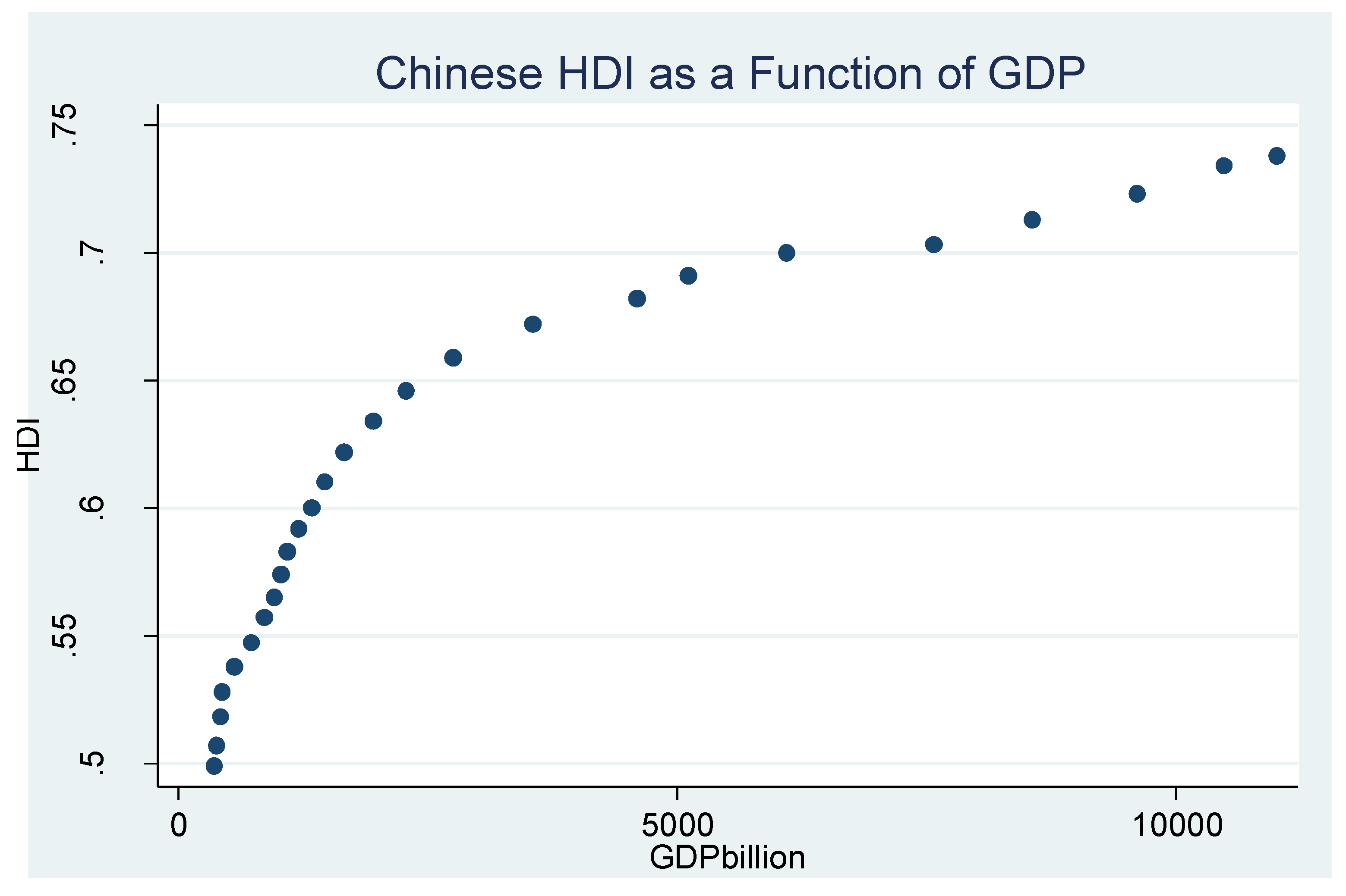
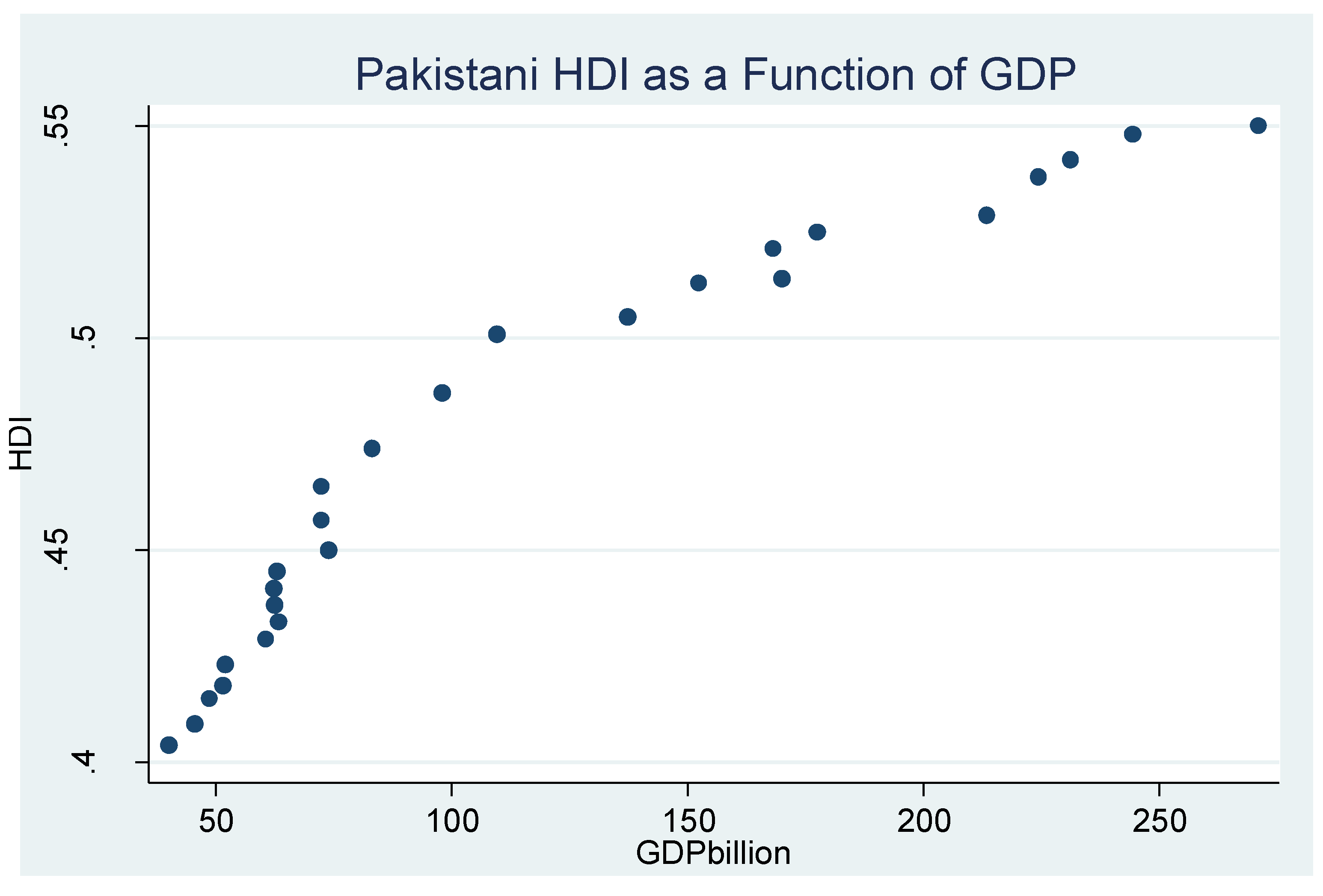
The elasticities in Table 5, like those in Table 3, demonstrate a sharply diminishing marginal utility for money in both Chinese and Pakistani societies. These tables support axiom 3, which posits H as an isoelastic power function of G. There is little change in H beyond its sizable increases driven by initial increments in G. This phenomenon is graphed in Figure 1 and Figure 2. The more precise Chinese function in Figure 1 is due to the higher indicator correlations for China in Table 4.
6. Conclusions
The present paper discovers three new properties of the gross domestic product in very different Asian economies:
First, Table 4 exhibits very high correlations over time among GDP indicators in China and Pakistan. Lemma 4 shows that this level of internal consistency implies near perfect correlations among all linear combinations of these indicators. Table 4 confirms, in particular, that Keynesian additive GDP is almost perfectly correlated over time with the first principal component G of the GDP indicators.
Second, this principal component G is in a class of weighted indexes ancillary to GDP. Each ancillary index informs policy as to allocation of resources over the three GDP indicators. The differential weighting of indexes like Gt is country specific, as is shown in Table 2 for China and Pakistan. The International Monetary Fund (IMF), especially sensitive to China’s global effects, noted that Chinese government policy is now “designated to accelerate the transformation of the Chinese economic model, improve livelihoods, and raise domestic consumption” (Singh et al. 2013). The generalized principal components analysis in Table 2 confirms the needed reallocation of Chinese GDP from gross domestic savings to household consumption. This finding illustrates how weighted indexes like Gt = a1Gt1 + a2Gt2 + a3Gt3 can inform governments about their GDP allocation. It also raises new questions as to which weighting of Gt1, Gt2, and Gt3 is most informative to policy. The latent 2-level principal components analysis in Section 4.2 selects Gt = a1Gt1 + a2Gt2 + a3Gt3 in Lemma 3, where a1, a2, and a3 are exhibited in Table 2 for China and Pakistan. This optimal internal weighting (a1, a2, a3) differs from that of an index that weights Gt1, Gt2, and Gt3 to maximize the prediction of external criteria. Nonetheless, alternative policy guidance is given by an external index that also has near perfect time-series correlation with unweighted GDPt = Gt1 + Gt2 + Gt3.
Third, a country-specific power of GDP almost perfectly predicts HDI. This finding is brought by regression analyses of time-series supplied by the World Bank and the United Nations. It is concluded that axiomatic HDI computation can be carried out in China and Pakistan without survey sampling, probabilistic inference, significance testing, or even HDI data.
Finally, the open problem of sustained GDP growth has been studied by the Leeds UK Steady State Economy Conference (O’Neill et al. 2010), the United Nations Division for Sustainable Development (Costanza et al. 2012), and the Annual Forum of The Progressive Economy Initiative (Journal for a Progressive Economy 2015). This problem has also been addressed by the Sarkozy report, which ends with the admonition that “no limited set of figures can pretend to forecast the sustainable or unsustainable character of a highly complex system” (Stiglitz et al. 2010, p. 136). Alperovitz envisions the present “political, ecological, and economic” system to be “the prehistory of transformative and fundamental systemic change. … Sustainability requires … a transformative vision beyond both corporate capitalism and traditional state socialism.” (Alperovitz 2017) (Italics mine).
Acknowledgments
This article is dedicated to the memory of Clyde Coombs who introduced the author to latent population distributions. The author thanks the editors and reviewers for their guidance and suggestions, which have improved the content and presentation of this work.
Conflicts of Interest
The author declares no conflict of interest.
Appendix A. Axiomatic Computation of Population Parameters
Axiomatic computation (rather than estimation) of population parameters is carried out on the three time-series of GDP indicators supplied by the World Bank (http://beta.data.worldbank.org). The findings in Table 1 and Table 2 are brought by the latent 2-level principal components analysis in Section 4.2.
The first of the following Stata commands (Stata Corp 2011) lists the three dollar-denominated GDP indicators in Section 2:
- pca hhspend savings govspend [fweight = popt], covariance
- estat kmo
- predict G
This first command operates on a 26 × 4 spreadsheet with rows labeled 1990 through 2015 and columns labeled population, household expenditure, gross domestic savings, and government expenditure. popt is population size, calibrated in millions, over 26 successive populations in years 1990 through 2015. The optional qualifier [fweight = popt] popt weights variables hhspend, savings, and govspend, expanding them to run over i = 1,…, popt for t = 1990,…, 2015. The option covariance calls for a principal components analysis of the covariance matrix of these three expanded variables, which are all measured in billions of current US dollars.
The second command computes the Kaiser-Meyer-Olkin parameter, which measures the common variance among the GDP indicators in Section 2.
The third command gives the first principal component G of hhspend, savings, and govspend. G is also measured in billions of current US dollars.
References
- Alperovitz, Gar. 2017. Principles of a Pluralist Commonwealth. The Next System Project. Available online: http://thenextsystem.org/principles/ (accessed on 15 March 2018).
- Bechtel, Gordon. 2017. New Unidimensional Indexes for China. Mathematical and Computational Applications 22: 13. [Google Scholar] [CrossRef]
- Coombs, Clyde H. 1950. Psychological scaling without a unit of measurement. Psychological Review 57: 145–58. [Google Scholar] [CrossRef] [PubMed]
- Coombs, Clyde H. 1964. A Theory of Data. New York: John Wiley & Sons. [Google Scholar]
- Costanza, Robert, Gar Alperovitz, Herman Daly, Joshua Farley, Carol Franco, Tim Jackson, Ida Kubiszewski, Juliet Schor, and Peter Victor. 2012. Building a Sustainable and Desirable Economy-in-Society-in-Nature. New York: United Nations Division for Sustainable Development. [Google Scholar]
- Ferrara, Antonella Rita, and Rosanna Nisticò. 2013. Well-being indicators and convergence across Italian regions. Applied Research in Quality of Life 8: 15–44. [Google Scholar] [CrossRef]
- Ferrara, Antonella Rita, and Rosanna Nisticò. 2015. Regional well-being indicators and dispersion from a multidimensional perspective: Evidence from Italy. The Annals of Regional Science 55: 373–420. [Google Scholar] [CrossRef]
- Johnston, John. 1984. Econometric Methods, 3rd ed. New York: McGraw-Hill. [Google Scholar]
- Journal for a Progressive Economy. 2015. Sustainable Growth: The Challenge of Transition. Annual Forum, June 2015. Brussels: The Progressive Economy Initiative. [Google Scholar]
- Keynes, John Maynard. 1936. The General Theory of Employment, Interest and Money. New York: Harcourt, Brace & World. [Google Scholar]
- Keynes, John Maynard. 1940. How to Pay for the War. London: Macmillan. [Google Scholar]
- Luce, Robert Duncan. 1959a. On the Possible Psychophysical Laws. Psychological Review 66: 81–95. [Google Scholar] [CrossRef]
- Luce, Robert Duncan. 1959b. Individual Choice Behavior: A Theoretical Analysis. New York: John Wiley & Sons. [Google Scholar]
- Luce, Robert Duncan, and Eugene Galanter. 1963. Psychophysical Scaling. In Handbook of Mathematical Psychology. Edited by Robert Duncan Luce, Robert R. Bush and Eugene Galanter. New York: John Wiley & Sons, vol. 1, pp. 245–307. [Google Scholar]
- Marchante, Andrés J., Bienvenido Ortega, and José Sánchez. 2006. The evolution of well-being in Spain (1980–2001): A regional analysis. Social Indicators Research 76: 283–316. [Google Scholar] [CrossRef]
- Masood, Ehsan. 2016. The Great Invention: The Story of GDP and the Making and Unmaking of the Modern World. New York: Pegasus Books Ltd. [Google Scholar]
- Nordhaus, William, and James Tobin. 1972. Is Growth Obsolete? In Economic Research: Retrospect and Prospect, Economic Growth. Edited by William Nordhaus and James Tobin. Cambridge: NBER, vol. 5, pp. 1–80. Available online: http://www.nber.org/chapters/c7620.pdf (accessed on 15 March 2018).
- OECD. 2017. How’s Life? 2017: Measuring Well-Being. Paris: OECD Publishing, Available online: http://dx.doi.org/10.1787/how_life-2017-en (accessed on 4 February 2018).
- O’Neill, Dan, Rob Dietz, and Nigel Jones, eds. 2010. Enough Is Enough: Ideas for a Sustainable Economy in a World of Finite Resources. The Report of the Steady State Economy Conference. Leeds: Center for the Advancement of the Steady State Economy and Economic Justice for All. [Google Scholar]
- Samuelson, Paul A., and William Nordhaus. 1985. Economics, 12th ed. New York: McGraw-Hill. [Google Scholar]
- Singh, Anoop, Malhar Nabar, and Papa M. N’Diaye, eds. 2013. China’s Economy in Transition: From External to Internal Rebalancing. Washington, DC: International Monetary Fund, Available online: http://www.elibrary.imf.org/page/chinatransition (accessed on 25 October 2017).
- Stata Corp. 2011. Stata Statistical Software, Release 12. College Station: Stata Corp LP. [Google Scholar]
- Stiglitz, Joseph E., Amartya Sen, and Jean-Paul Fitoussi. 2010. Mismeasuring Our Lives: Why GDP Doesn’t Add up: The Report of the Commission on the Measurement of Economic Performance and Social Progress. New York: New Press. [Google Scholar]
Figure 1.
Human Development Index (HDI) is in [0, 1] and GDP is in billions of dollars.

Figure 2.
HDI is in [0, 1] and GDP is in billions of dollars.


Table 1.
Eigenvalues for G.
| Principal Components | 1 | 2 | 3 |
|---|---|---|---|
| Chinese eigenvalues | 4,783,248 | 6795 | 98 |
| Pakistani eigenvalues | 3841 | 6 | 1 |
Note. The proportions of indicator variance accounted for by the first principal components are 0.9986 in China and 0.9982 in Pakistan. Each proportion equals the first eigenvalue divided by the sum of that nation’s three eigenvalues.
Table 2.
First eigenvectors for G.
| Nation | Household Consumption | Gross Domestic Savings | Government Consumption |
|---|---|---|---|
| China | 0.5712 | 0.7939 | 0.2087 |
| Pakistan | 0.9898 | 0.0700 | 0.1245 |
Note. The squared scoring coefficients in each row sum to one.
Table 3.
Regressions of lnH on lnG.
| Nation | Slope (Elasticity) | R2 |
|---|---|---|
| China | 0.1088 | 0.9818 |
| Pakistan | 0.1553 | 0.9717 |
Table 4.
Correlations of Nt-weighted indicators, G, and Nt-weighted GDPt.
| Indicator | China | Pakistan | ||
|---|---|---|---|---|
| Gt2 | Gt3 | Gt2 | Gt3 | |
| Gt1 | 0.9968 | 0.9996 | 0.8836 | 0.9859 |
| Gt2 | 0.9977 | 0.8367 | ||
| r(G, GDP) = 1.0000 | r(G, GDP) = 0.9997 | |||
Table 5.
Regressions of lnH on ln{Nt-weighted GDPt}.
| Nation | Slope (Elasticity) | R2 |
|---|---|---|
| China | 0.1102 | 0.9818 |
| Pakistan | 0.1662 | 0.9718 |
© 2018 by the author. Licensee MDPI, Basel, Switzerland. This article is an open access article distributed under the terms and conditions of the Creative Commons Attribution (CC BY) license (http://creativecommons.org/licenses/by/4.0/).
Share and Cite
MDPI and ACS Style
Bechtel, G. The Human Development Index as Isoelastic GDP: Evidence from China and Pakistan. Economies 2018, 6, 32. https://doi.org/10.3390/economies6020032
AMA Style
Bechtel G. The Human Development Index as Isoelastic GDP: Evidence from China and Pakistan. Economies. 2018; 6(2):32. https://doi.org/10.3390/economies6020032
Chicago/Turabian StyleBechtel, Gordon. 2018. "The Human Development Index as Isoelastic GDP: Evidence from China and Pakistan" Economies 6, no. 2: 32. https://doi.org/10.3390/economies6020032
Note that from the first issue of 2016, this journal uses article numbers instead of page numbers. See further details here.