A New Quota Approach to Electoral Disproportionality


1
PRESAD Research Group, BORDA Research Unit, IMUVa, Departamento de Economía Aplicada, Universidad de Valladolid, 47011 Valladolid, Spain
2
PRESAD Research Group, Unidad Académica de Matemáticas, Universidad Autónoma de Zacatecas, Zacatecas 98000, Mexico
3
Departamento de Matemática Aplicada, Universidad de Granada, 18071 Granada, Spain
*
Author to whom correspondence should be addressed.
Economies 2019, 7(1), 17; https://doi.org/10.3390/economies7010017
Submission received: 10 January 2019
/
Revised: 22 February 2019
/
Accepted: 26 February 2019
/
Published: 5 March 2019
(This article belongs to the Special Issue Public Choice)
Abstract
:In this paper electoral disproportionality is split into two types: (1) Forced or unavoidable, due to the very nature of the apportionment problem; and (2) non-forced. While disproportionality indexes proposed in the literature do not distinguish between such components, we design an index, called “quota index”, just measuring avoidable disproportionality. Unlike the previous indexes, the new one can be zero in real situations. Furthermore, this index presents an interesting interpretation concerning transfers of seats. Properties of the quota index and relationships with some usual disproportionality indexes are analyzed. Finally, an empirical approach is undertaken for different countries and elections.
1. Introduction
Electoral systems are mechanisms by which votes become seats in a parliament. In order to reflect the overall distribution of voters’ preferences, some of these systems advocate for proportional representation, so that political parties will receive percentages of seats corresponding to their respective percentages of votes. Since a seat cannot be divided, it is impossible to assign exactly the obtained vote shares in seat terms. This apportionment problem generates something known as electoral disproportionality. Consequently, some parties are overrepresented while others become underrepresented. Even more, disproportionality may increase, due to the existence of many districts and electoral thresholds.
There is not an agreement about an instrument to determine such distortions generated during the process of translating votes into seats and many efforts have been made to measure them. Disproportionality indexes are usually employed to this aim and there exists a wide literature on this approach.
A survey compilation of indexes resulting from the application of different techniques is presented by Taagepera and Grofman (2003) (see also Taagepera 2007; Karpov 2008; Chessa and Fragnelli 2012; Goldenberg and Fisher 2017). These authors also develop an interesting analysis of the properties that they fulfill. From a computational point of view, Ocaña and Oñate (2011) presents a software for calculating nine disproportionality indexes. On the other hand, Koppel and Diskin (2009) and Boyssou et al. (2016) propose axiomatizations for some indexes measuring disproportionality. Finally, relationships among some disproportionality indexes appear in Borisyuk et al. (2004) and Bolun (2012).
All the proposed indexes measure deviations (in some way) from exact proportionality, which is not affordable in practice. Balinski and Young (2001, pp. 79–83) deals with a more realistic requirement concerning the apportionment problem: No party’s representation should deviate from its quota (number of seats that should be received by the parties in exact proportionality) by more than one unit. In other words, no party should get less than its quota rounded down, nor more than its quota rounded up. This property is called “staying within the quota” or “verification of the quota rule”. Taking into account that usually the quota is not an integer number, votes-seats disproportionality could be non-forced (if the quota rule is not satisfied), or forced, otherwise.
This paper presents a new index that just measures non-forced disproportionality, avoiding that inherent to the fact that exact proportionality is unfeasible, as pointed out. Remarkably, this index is zero if and only if the quota condition is satisfied. Even more, from this index, it is possible to obtain the minimum number of seats that would be necessary to transfer from some parties to others, so that the distribution of parliament seats will satisfy the quota condition.
The paper has the following structure: Section 2 introduces the notation and basic concepts, paying particular attention to the quota. Section 3 presents some of the most used disproportionality indexes, namely: The maximum deviation, Loosemore-Hanby and Gallagher indexes. Section 4 introduces a new index, which will be called “quota index”. Section 5 shows the properties that the last index verifies and some relationships with the previous disproportionality indexes. In Section 6 the aforementioned indexes are computed for different elections in Spain, Sweden and Germany, and comparisons among them are established. In Section 7, some conclusions are presented. Finally, technical proofs, electoral results and data resources are left in Appendix A, Appendix B and Appendix C, respectively.
2. Notation and Basic Concepts
Let be the number of voters, the number of parties and the number of seats to be distributed; is the vector whose components are the votes obtained by each party, so that ; on the other hand, is the vector whose components are the seats assigned to each party, where ; finally, we denote by and the proportion of votes and seats that party receives. Thus, and are the vote and seat shares, respectively, for each party .
A party is overrepresented when , and underrepresented when . Any of these inequalities represents a distortion with respect to the voters’ real preferences.
The quota (or “fair share”) is the number of seats that the party should receive in exact proportionality after obtaining votes. That is, the quota for party results .
In terms of the quota, a party is underrepresented if and overrepresented if . Since , if a party is underrepresented, at least another one will be overrepresented.
The lower quota is the closest integer number that does not exceed ; it will be denoted by . Likewise, the upper quota is the smallest integer number bigger than or equal to ; it will be denoted by . In other terms, the lower quota is obtained by rounding down and the upper quota by rounding up .
Usually, for each party, quotas are fractional numbers and hence Otherwise, if is an integer number, then . The interval whose extremes are lower and upper quotas will be called quota interval.
An apportionment satisfies the quota rule if the number of seats assigned to each party differs from its quota less than one, this is: or equivalently, for each .
On the other hand we will say that a party is overrepresented with respect to the upper quota if and is underrepresented with respect to the lower quota if Obviously, these are more restrictive requirements for parties than being merely overrepresented or underrepresented.
3. Some Indexes of Electoral Disproportionality and Their Relationship
The literature on indexes is devoted to measuring the quality of an electoral system, in some way. One of the most important issues in this context is electoral disproportionality, which could be defined as the deviation level of vote and seat shares of the participating parties in an election.
In order to determine electoral disproportionality various indexes have been proposed. As aforementioned, compilations of these indexes have been made by different authors (Taagepera and Grofman 2003; Karpov 2008). Among them, the maximum deviation index, the Loosemore-Hanby index proposed by Loosemore and Hanby (1971) and the least squares index, presented by Gallagher (1991), are some of the most frequently used ones.
3.1. Maximum Deviation Index
This index measures the maximum difference between vote and seat shares in absolute terms. The mathematical expression for this index is:
As it can be observed, the maximum deviation index only provides information of one party that can be either the most underrepresented or overrepresented one, regardless of the deviation sizes of the other parties.
3.2. Loosemore-Hanby Index
This index adds all the deviations generated during the allocation, meaning the sum of absolute values of the differences between the vote and seat shares. Mathematically the index is defined as
The sum of absolute values of the differences between the vote and seat shares for overrepresented parties coincides with the same sum for underrepresented ones. Hence, the total sum appearing in is divided by two in order to obtain the seat share that has not been distributed in a completely proportional way.
3.3. Gallagher Index
The least squares index is also known as Gallagher index, and it is defined as the square root of the sum of the squared differences between vote and seat shares of every party divided by two. Formally:
This index takes into account both big and small deviations in the proportion of assigned seats and obtained votes. However, small differences have less influence than big differences. Consequently, this index is less sensitive than the previous one to the appearance of small parties.
3.4. Relationship among Disproportionality Indexes
Obviously, if and only if there exists exact proportionality, i.e., the percentage of votes equals that of seats for each party. Some further relations among these indexes can be established. It is straightforward that if and only if there exists either just one overrepresented or just one underrepresented party. On the other hand, if there are at least two overrepresented parties jointly with another two underrepresented ones, it is straightforward that .
On the other hand, Borisyuk et al. (2004) proved that . Besides, it is easy to check that if and only if there is exactly one overrepresented party jointly with just one underrepresented party. In both cases, also reaches the same value.
Finally, taking into account the aforementioned relationships concerning the considered indexes we can assert that, if there are at least two overrepresented parties jointly with another two underrepresented ones, then .
4. The Quota Index
All the aforementioned indexes measure deviations between vote and seat shares, and hence, in an implicit way, they take into account the quota as a point of reference. For example, the Loosemore-Hanby index can be expressed in quota terms as
Note that if and only if for all the parties (this is also true for the previously considered indexes). However, as the seats are indivisible, this situation requires all to be integer numbers, and this is extremely unlikely. Therefore, exact proportionality becomes almost impossible in real elections.
On the other hand, in terms of seat transference can be understood as the proportion of seats that we need to transfer from overrepresented parties to underrepresented ones in order to achieve exact proportionality. However, this is merely a theoretical value because, again, such exact proportionality would require the seats to be divided.
This is the reason why we have focused our attention not in exact apportionments, but in those staying within the quota, which is a more plausible condition. These considerations do not mean that we advocate for apportionment methods verifying the quota rule, as the largest remainders (a.k.a. Hamilton) rule. That is, regardless of the used method, our aim is measuring post hoc deviations from the quota interval.
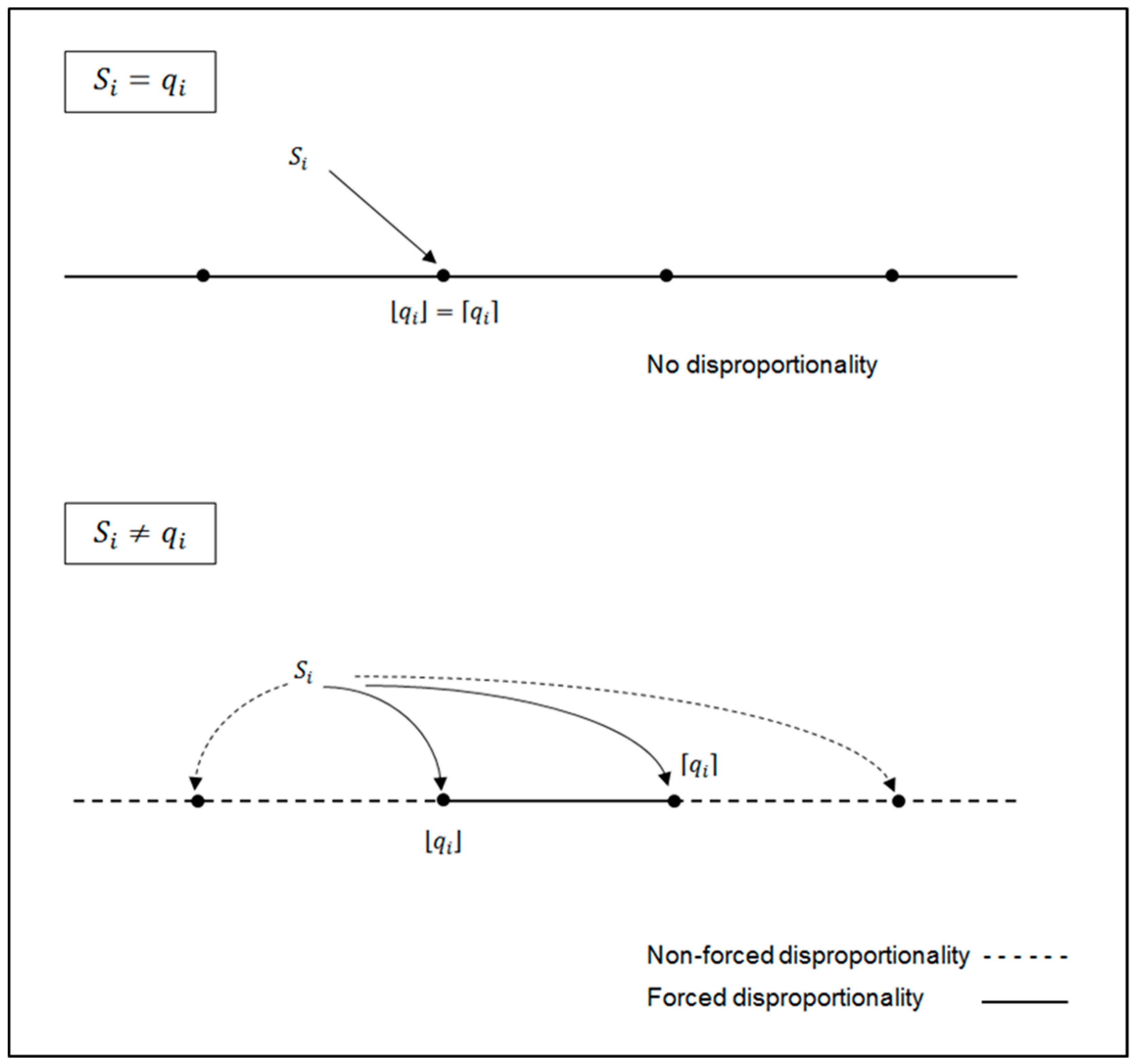
If the quota is not an integer number for some party, depending on the value of two kinds of disproportionality can be considered. We will say that in an allocation of seats, there exists non-forced disproportionality if some party does not verify the quota condition (i.e., it is overrepresented with respect to the upper quota or underrepresented with respect to the lower quota). Otherwise, the quota rule is satisfied for all the parties and we will talk about forced disproportionality, unavoidable due to the nature of the apportionment problem. Such considerations are illustrated in Figure 1.
These ideas have been taken into account in our proposal, in which we only measure non-forced disproportionality (i.e., beyond de quota interval): That is, only distances of overrepresented parties from their upper quotas or underrepresented parties from their lower quotas are considered. In this way, we have defined an index, called quota index, as
The value of is between zero and one. The zero value corresponds to any distribution that verifies the quota rule, while the maximum disproportionality will be reached when all the seats are assigned to parties with no votes. It is worth noting that, while Loosemore-Hanby and the other aforementioned indexes are zero if and only if the apportionment is exact, can be zero without this requirement. But, obviously, is also zero if there exists exact proportionality.
Moreover, our index has an interesting interpretation in transference terms: The quota index is the minimum proportion of seats in a parliament of seats that we would need to transfer from overrepresented parties with respect to the upper quota to others underrepresented (or from overrepresented parties to others underrepresented with respect to the lower quota), for the quota rule to be verified. And will be exactly the minimum number of seats that would have to be transferred from some parties to others for the distribution to verify the quota condition at a global level. This fact will be illustrated in Section 6 concerning 2016 Spanish elections.
5. Quota Index Analysis and Relationships with Other Indexes
Karpov (2008), Taagepera and Grofman (2003) and Taagepera (2007) propose some reasonable properties and analyze their fulfillment for several disproportionality indexes, the maximum deviation, the Loosemore-Hanby index and the Gallagher indexes among them. In this section, after showing the difference of perspectives between the above-mentioned indexes and the new one, we will test for the most relevant properties appearing in the literature.
In what follows, we will formulate the above-mentioned disproportionality indexes in terms of the quota. In Section 4 we have shown that:
In a similar way, it is easy to check that:
and
These expressions are intended to establish in an easy way their relationships with the quota index. It will be also used in further computations.
5.1. Quota Index and Disproportionality Indexes: Difference of Scopes
In Section 4, disproportionality has been split into two types. As shown in the previous expressions, traditional approaches to this issue measure the distances from quotas, and hence they take into account both forced and non-forced disproportionality. On the other hand, the quota index just measures distances to the quota interval, and therefore just consider non-forced disproportionality. In other words, usual disproportionality indexes contemplate underrepresented on overrepresented parties, while the quota index just considers those over the upper quota or below the lower quota.
The following example illustrates these aspects.
Example 1.
Consider parties A and B, and let the number of seats to allocate. Suppose thatandare the number of seats and the respective quota of the party A. Also consider thatandare the number of seats and the quota of the party B, respectively. Then, we obtain:
However, as the quota rule is verified,Notice that with these data all the appearing disproportionality is forced (unavoidable).
5.2. Disproportionality Indexes Properties and Quota Index
- Anonymity: Any permutation of party labels does not change the value of the index.
- Principle of transfers: If we transfer a seat from an overrepresented party to an underrepresented one, then the value of the index should not increase.
- Independence from split: Suppose there are many parties with equal vote and seat shares, and these parties are grouped into one. Then, the value of the index calculated for all the parties in the group should be equal to the value of the index for the group considered as a whole.
- Scale invariance (homogeneity): The index should not depend on any proportional change in the number of votes or seats
- Zero normalization: This property is satisfied if, when for all then the value of the index is 0.
Next, we will check the fulfillment of the previous properties by .
Proposition 1.
The indexsatisfies anonymity, principle of transfers and zero normalization.
(The proof can be found in Appendix A).
Now, Example 2 shows that does not satisfy the property of independence from split.
Example 2.
Suppose nine parties whose quotas and assigned seats appear in Table 1, where
Calculating separatelyfor all the appearing parties, we obtain:
Now, in Table 2,is calculated for parties with equal percentage of seats and quotas as unique coalitions:
And hence
Table 3 shows the properties that , , and satisfy or do not (Karpov (2008) and Taagepera and Grofman (2003) for the three first indexes). A “+” sign means that the index satisfies the property and “−” means that it does not. Occasionally, these signs may appear enclosed into parentheses to point out that the corresponding property is or not satisfied under specific circumstances.
Parentheses appearing in the column relative to the Principle of Transfers in Table 3 mean that , and may violate the principle of transfers in some situations, as shown in Example 3.
Example 3.
Consider partiesand, and. Suppose thatand. That is,is overrepresented andis underrepresented. In this situation:
Now, if we transfer a seat fromto
Note that, in this example, after the seat transference the overrepresented party becomes underrepresented, and vice versa.
However, it is easy to check that , and satisfy a weaker Principle of Transfers establishing that, if a seat is transferred from an overrepresented party verifying to an underrepresented one that satisfies , then the value of these indexes should not increase. In particular, this situation happens when a seat is transferred from an overrepresented party with respect to the upper quota to an underrepresented one with respect to the lower quota. Concerning different versions of the Principle of Transfers in electoral disproportionality and their connection with the original Dalton’s Principle in more general inequality contexts, see Taagepera and Grofman (2003), Van Puyenbroeck (2008) and Goldenberg and Fisher (2017).
On the other hand, the parentheses appearing in the column relative to Scale Invariance in Table 3 means that violates this property just with proportional changes in the number of seats, but not in the number of votes, as shown in Example 4.
Example 4.
Consider again partiesand, and. Suppose thatand. Note that in this situation the quota rule is satisfied and henceIf we multiply by 10 the number of seats, that is,, we obtainand. Now, the quota rule is not verified and.
However, this fact should not be considered as a drawback of the index because the first situation cannot be improved by transferring seats in any way, while in the second situation if we transferseats from party A to B, the quota rule is verified. Even more, in this case the apportionment becomes exact.
Concerning this issue, Boyssou et al. (2016) assert that although the homogeneity with respect the number of seats “seems rather reasonable for large parliaments, a good disproportionality index should perhaps be sensitive to the size of the parliament, at least for small parliaments”.
Obviously, proportional changes in the number of votes (maintaining the number of seats to allocate) do not affect the quota and consequently neither the value of .
Some other properties can be considered for a disproportionality index (Taagepera and Grofman 2003; Taagepera 2007), among them:
- Informationally complete (makes use of all and )
- Uses data for all parties uniformly
- Does not depend on the number of parties
- Varies between 0 and 1 (or 100%)
As shown by the previous authors, these properties are satisfied by the disproportionality indexes considered along this paper, except the first one by . On the other hand, it is straightforward that also verifies all of them.
5.3. Relationships among and Disproportionality Indexes
The relationships existing among different disproportionality indexes have been shown in various ways (Borisyuk et al. 2004; Bolun 2012). In the present paper some relationships that the quota index has with the disproportionality indexes appearing above will be analyzed.
Proposition 2.
The value of the quota index is always minor than or equal to the Loosemore-Hanby index:
(The proof can be found in Appendix A).
Proposition 3.
The values of the quota and the maximum deviation indexes verify the following inequality:
(The proof can be found in Appendix A).
Obviously, if there exists exact proportionality. If not, other relations can be established. It is obvious that if and only if are integer numbers for all the overrepresented parties and the maximum of the expression of is reached for these ones, or are integer numbers for all the underrepresented parties and the maximum is reached for them. As these situations are extremely unlikely, in general .
On the other hand, it is straightforward that if and only if there exists either just one overrepresented party with respect to the upper quota and, in addition, its quota is an integer number or just one underrepresented party with respect to the lower quota and, in addition, its quota is an integer.
Finally, it is easy to check that if there is just one overrepresented party whose quota is an integer number and, in addition, there is exactly one underrepresented party. In both cases, also reaches the same value. Otherwise both inequalities might appear between and . For example, in any allocation verifying the quota with no exact proportionality, . But if the quota condition is not satisfied, the inequality might be reversed and, in fact, is unlikely (see results in Section 6).
5.4. Discussion about Indexes
It can be observed that, as appearing in Table 3, none of the indexes considered along the paper is optimal. This situation is somehow analogous (in another context) to those in Social Choice theory, where is well known that there do not exist perfect voting systems nor apportionment methods, as proven by Arrow and Balinski-Young theorems, respectively.
In fact, it is possible to find examples where all the considered indexes present some weaknesses, as will be shown in what follows.
In an electoral situation where there exist non integer quotas (in fact, this is the most usual case), it is impossible to achieve exact proportionality, but it is always possible to find an apportionment verifying . It is a simple question of adjustment of each in its quota interval, so that, at the end of the process . In such a situation, there are several possibilities of seat distribution staying within the quota, and this fact might be considered as a criticism, as shown in Example 5.
Example 5.
Consider parties A and B, and let the number of seats to allocate. Suppose thatandIn this situation there are two possibilities of seat distribution staying within the quota:,and,. Hence,.
However, the second allocation is less compelling than the first one, because the most voted party obtains the least representation. In other terms, there exists a lack of vote/seat monotonicity in the last apportionment.
Now, notice that for the first allocation, we have, while for the second allocation,. Consequently, these indexes point out the first allotment as better than the second one.
Nonetheless, Example 6 illustrates that the lack of monotonicity might not be captured (even more, it can be inversely reflected) when the usual disproportionality indexes are used.
Example 6.
Suppose eight parties whose quotas and assigned seats (in two different apportionments) appear in Table 4, where.
The first seat distribution is intentionally arbitrary (in fact, it cannot be obtained by any divisor or quotient method). However, the second distribution is obtained by any divisor method in the parametric family (Balinski and Victoriano 1999) between Webster (Sainte-Laguë) and Jefferson (D’Hondt).
After some computations, the obtained values for quota and maximum deviation indexes in both allotments areandThe first apportionment presents two pair of parties,and, where, in each of them, the most voted is the least represented. However, in this example, unlike the previous one, Loosemore-Hanby and Gallagher do no detect this lack of monotonicity. Even worse, they work in the opposite way to that expected:and
6. Implementation of the Quota Index in Some Countries and Elections
We first study in depth the case of Spain along the last 25 years, paying special attention to the transfer analysis in the 2016 elections, as well as to the overall correlation of the disproportionality indexes previously calculated.
Afterwards, we merely calculate the considered indexes for another two countries, Sweden and Germany, jointly with some comments on the results.
As a caveat, we note that slight (and hence negligible) differences might appear in the results, due to the treatment (grouped or not) of small parties without representation.
All electoral data resources appear in Appendix C.
6.1. Spain (1993–2016)
In Spain there exists a party list proportional representation system. The Spanish Chamber of Deputies has 350 members chosen in 52 districts. An exclusion threshold of 3% of the valid votes in each district is applied. All these elements have not been modified from 1977. Disproportionality partially occurs in Spain because population/representation shares are not balanced among districts. Furthermore, due to the small size of districts, some parties whose votes are scattered all over the country may obtain significantly fewer seats than other parties with a similar number of votes, if geographically concentrated. Other causes of disproportionality in Spain are the use of the D’Hondt rule, intended to favor larger parties.
Table 5 shows the values of maximum deviation, Loosemore-Hanby, Gallagher and the quota indexes for the eight most recent elections in Spain.
In all analyzed elections, is bigger than (as theoretically proven), while is the smallest (hence, in particular, in all the cases). Remarkably, the quota rule never is globally satisfied, given that always .
Focusing our attention in 2016, it can be observed that all the obtained values have decreased from those corresponding to the previous elections. An important fact that can partially explain this issue is that IU, a left-wing party, traditionally penalized by vote dispersion, formed a coalition with the emergent party Podemos.
Following with the last Spanish elections, it is worth noting that and This value corresponds to the number of seats to be transferred from some parties to others in order to achieve exact proportionality. This is a theoretical value because seats cannot be divided. On the other hand, , and hence , which means that this is the minimum number of seats to be transferred for the apportionment to verify the quota. This is a feasible goal. Concretely, in order to achieve this aim, 20 seats belonging to PP and 5 more seats from PSOE should be transferred to C’s (14), PACMA (4) and Podemos-IU-EQUO (2). The remaining 5 seats should be moved, one by one, to any other unrepresented party (see Appendix B for details).
Despite the fact that solely measures non-forced disproportionality and the remaining indexes are disproportionality ones, in what follows a correlation analysis among them is undertaken in order to explore their relationships. Table 6 shows the results coming from data appearing in Table 5.
The highest correlation value appears between and . This fact relies on the formal expression of which is somehow inspired by that of , although the first one only measures avoidable (beyond the quota interval) disproportionality. Hence, both indexes have different interpretations, as aforementioned. On the other hand, and .
6.2. Other Countries
As aforementioned, we next calculate the considered disproportionality indexes for another two countries, Sweden (proportional system) and Germany (mixed-member system).
6.2.1. Sweden (1998–2014)
Sweden is ranked in the third position worldwide according to the 2017 democratic index developed by The Economist Intelligence Unit (www.eiu.com). The Swedish Parliament (Riksdag) is composed of 349 seats elected under a proportional system. 310 of them belong to fixed constituency seats and the remaining 39 are adjustment seats. Any particular party must receive at least 4% of the national votes to be assigned a seat. Fixed seats are allocated among the parties using a method known as the adjusted odd numbers method (or modified Sainte-Laguë).
The purpose of the 39 adjustment seats is to make sure that the distribution of seats among the parties over the whole country should be as proportional in relation to the number of votes as possible. The whole country is viewed as it was a single constituency and is then compared with the distribution of votes in the 29 constituencies. The adjustment seats are allocated first according to party and then according to the constituency (see www.riksdagen.se for details).
Table 7 shows the values of the and indices in all the Swedish Riksdag elections held from 1998 to 2014.
It can be observed, as in the previously studied case, that is always between and . Notice also that now the obtained results are lower than those for Spain. In fact, the Swedish electoral system produces a high proportionality unless one or several political parties have a percentage of votes just a little below the electoral threshold (4%). Concretely, this situation happened in 2006 and 2014 because the Sweden Democrats and the Feminist Initiative parties obtained 2.9% and 3.1% of the national votes, respectively.
6.2.2. Germany (1976–2017)
Germany’s electoral system is a combination of “first-past-the-post” election of constituency candidates (first votes) and proportional representation on the basis of votes for the parties’ States (Länder) lists (second votes). Hence, it is a mixed-member electoral system.
Concretely, half of the Members of the German Parliament (Bundestag) are elected directly from Germany’s 299 constituencies, the other half via party lists in Germany’s sixteen Länder. Accordingly, each voter casts two votes in the elections to the German Bundestag. The first vote, allowing voters to elect their local representatives to the Bundestag, decides which candidates are sent to Parliament from the constituencies. The second vote is cast for a party list. The 598 seats are distributed among the parties that have gained more than 5% of the second votes or at least three constituency seats. Each party receives the minimum between the number of seats obtained on the basis of the first votes and those corresponding to the second votes. The Sainte-Laguë/Schepers method is used to convert the votes into seats
In some circumstances, Parliament’s size may increase during the process of allocating the seats, due to what are known as “overhang seats” and additional “balance seats” in order to maintain proportionality (see www.bundestag.de for further details).
Table 8 shows the values of the and indices in the German Bundestag elections held from 1976 to the most recent in 2017.
Notice that, again, the values of are always between those of and . Paying attention to the historical sequence of data, the magnitude of the results obtained in 2013 is shocking. This high disproportionality arose because, in this year, parties that did not overcome the electoral threshold represented approximately 16% of the votes.
7. Conclusions
In this paper, the quota index () has been introduced and analyzed. It is worth mentioning that this index is zero if and only if the quota rule is satisfied by all the parties, i.e., when only forced (i.e., unavoidable) disproportionality arises.
Remarkably, in our approach, can occur even if the apportionment is not exact (in fact, exact proportionality is almost impossible, due to the very nature of the apportionment problem). Moreover, corresponds to the minimum percentage of seats that is necessary to transfer among parties for the quota rule to be verified. From this value it is possible to obtain the minimum number of seats (being an integer number) that it would be necessary to transfer from some parties to others, so that the seat distribution of the parliament will satisfy the quota condition.
After an electoral process, it is usual for the main party to be overrepresented. If the underrepresentation is distributed among all the other parties and none of them stays below its lower quota, then will represent the surplus of the winning party calculated from its upper quota. Notice also that, contrary to other well-known disproportionality indexes, the existence of many small parties with a quota less than the unit and without seat representation do not increase the value of .
We have proven that the quota index verifies some compelling properties appearing in the literature. In particular, it is worth noting that gain an advantage over some of the most relevant disproportionality indexes (maximum deviation, Loosemore-Hanby and Gallagher) when the principle of transfers is considered. On the other hand, we have checked that the quota index is not homogenous with respect to the number of seats, although it has been justified that this fact can make sense in our context.
Finally, quantitative relationships have been established among the quota and the aforementioned disproportionality indexes and all of them have been calculated for several elections in Spain, Sweden and Germany. The obtained results show that there exists a high correlation among the Loosemore-Hanby and quota indexes, but a major argument to use the last one is its interpretability in terms of seat transfer.
Author Contributions
All the authors have equally participated in the research aspects of the work reported.
Funding
We are grateful for the financial support of the Spanish Ministerio de Economía y Competitividad (project ECO2016-77900-P).
Acknowledgments
The authors acknowledge and appreciate the comments of two anonymous referees.
Conflicts of Interest
The authors declare no conflict of interest.
Appendix A. Proofs of the Propositions
Proposition 1.
The indexsatisfies anonymity, principle of transfers and zero normalization.
Proof:
- Anonymity
Given that the value of is the maximum of two arguments:
this property is immediate since it relies on commutative property for real numbers.
- Principle of transfers
Consider and , number of seats assigned and quota for an overrepresented party , respectively. Let and be the number of seats assigned and the quota for an underrepresented party , respectively. When a seat is transferred from to , the following cases can happen:
- (1)
- If party continues being overrepresented, then
- (2)
- If party becomes underrepresented, then
In such scenarios we can find any of these situations:
- (a)
- If party continues being underrepresented, then
- (b)
- If party becomes overrepresented, then
Taking this into account, if a seat is transferred from an overrepresented party to an underrepresented one does not increase its value in any of the arguments of the maximum appearing in its expression.
- Zero normalization
If for all then and . Furthermore, we know that , because . Given that the number of assigned seats is an integer number and , is also an integer number, and then . Therefore:
Proposition 2.
The value of the quota index is always minor than or equal to the Loosemore-Hanby index:
Proof:
As aforementioned in Section 4, the Loosemore-Hanby index can be expressed in terms of the quota as
On one hand, given that the sum of the terms corresponding to overrepresented parties is equal to that corresponding to underrepresented ones, we obtain
On the other hand,
Thus, the maximum of the two terms appearing in the definition of is less than or equal to . □
Proposition 3.
The value of the quota indexes and the maximum deviation verify the following inequality:
Proof:
Taking into account that
we consider two cases:
- (a)
- If is reached for underrepresented party , then Therefore:where the last inequality takes into account that . Dividing both extreme members by , we have
- (b)
- If is reached for a party that is overrepresented, then Therefore:where the last inequality takes into account that . Dividing both extreme members by , we have
In consequence, . □
Appendix B.

Table A1.
Spanish Electoral Results (2016).
| Parties | Votes | Quotas | Seats |
|---|---|---|---|
| PP | 7906.185 | 116.48 | 137 |
| PSOE | 5424.709 | 79.92 | 85 |
| PODEMOS-IU-EQUO | 3201.170 | 47.16 | 45 |
| C’s | 3123.769 | 46.02 | 32 |
| ECP | 848.526 | 12.50 | 12 |
| PODEMOS-COMPROMÍS-EUPV | 655.895 | 9.66 | 9 |
| ERC-CATSÍ | 629.294 | 9.27 | 9 |
| CDC | 481.839 | 7.10 | 8 |
| PODEMOS-EN MAREA-ANOVA-EU | 344.143 | 5.07 | 5 |
| EAJ-PNV | 286.215 | 4.22 | 5 |
| EH Bildu | 184.092 | 2.71 | 2 |
| CCa-PNC | 78.080 | 1.15 | 1 |
| PACMA | 284.848 | 4.20 | |
| RECORTES CERO-GRUPO VERDE | 51.742 | 0.76 | |
| UPyD | 50.282 | 0.74 | |
| VOX | 46.781 | 0.69 | |
| BNG-NÓS | 44.902 | 0.66 | |
| PCPE | 26.553 | 0.39 | |
| GBAI | 14.289 | 0.21 | |
| EB | 12.024 | 0.18 | |
| FE de las JONS | 9.862 | 0.15 | |
| SI | 7.413 | 0.11 | |
| SOMVAL | 6.612 | 0.10 | |
| CCD | 6.264 | 0.09 | |
| PH | 3.288 | 0.05 | |
| SAIn | 3.221 | 0.05 | |
| P-LIB | 3.103 | 0.05 | |
| CENTRO MODERADO | 2.986 | 0.04 | |
| CCD-CI | 2.668 | 0.04 | |
| UPL | 2.307 | 0.03 | |
| PCOE | 1.812 | 0.03 | |
| AND | 1.695 | 0.02 | |
| JXC | 1.184 | 0.02 | |
| IZAR | 854 | 0.01 | |
| CILUS | 847 | 0.01 | |
| PFyV | 838 | 0.01 | |
| PxC | 722 | 0.01 | |
| MAS | 718 | 0.01 | |
| UNIDAD DEL PUEBLO | 684 | 0.01 | |
| PREPAL | 640 | 0.01 | |
| Ln | 617 | 0.01 | |
| REPO | 569 | 0.01 | |
| INDEPENDIENTES-FIA | 556 | 0.01 | |
| IMC | 351 | 0.01 | |
| FME | 338 | 0.00 | |
| PUEDE | 330 | 0.00 | |
| ENTABAN | 257 | 0.00 | |
| FE | 254 | 0.00 | |
| ALCD | 210 | 0.00 | |
| HRTS-Ln | 82 | 0.00 | |
| UDT | 54 | 0.00 | |
| Total | 23,756.674 | 350 | 350 |
Source: Ministry of Interior (Spain).
Appendix C. Electoral Data Resources
Sweden: www.electionresources.org/se/.
References
- Balinski, Michael, and Victoriano Ramírez. 1999. Parametric methods of apportionment, rounding and production. Mathematical Social Sciences 37: 107–22. [Google Scholar] [CrossRef]
- Balinski, Michael, and H. Peyton Young. 2001. Fair Representation: Meeting the Ideal of One Man, One Vote. Washington, DC: Brookings Institution Press. [Google Scholar]
- Bolun, Ion. 2012. Comparison of indices of disproportionality in PR systems. Computer Science Journal of Moldova 20: 246–71. [Google Scholar]
- Borisyuk, Galina, Colin Rallings, and Michael Thrasher. 2004. Selecting indexes of electoral proportionality: General properties and relationships. Quality and Quantity 38: 51–74. [Google Scholar] [CrossRef]
- Boyssou, Denis, Marchant Thierry, and Marc Pirlot. 2016. Axiomatic Characterization of Some Disproportionality and Malapportionment Indices. Available online: https://editorialexpress.com/cgi-bin/conference/download.cgi?db_name=SCW2016&paper_id=287 (accessed on 7 January 2019).
- Chessa, Michela, and Vito Fragnelli. 2012. A note on Measurement of disproportionality in proportional representations systems. Mathematical and Computer Modelling 55: 1655–60. [Google Scholar] [CrossRef]
- Gallagher, Michael. 1991. Proportionality, disproportionality and electoral systems. Electoral Studies 10: 33–51. [Google Scholar] [CrossRef]
- Goldenberg, Josh, and Stephen D. Fisher. 2017. The Sainte-Laguë index of disproportionality and Dalton’s principle of transfers. Party Politics. [Google Scholar] [CrossRef]
- Karpov, Alexander. 2008. Measurement of Disproportionality in Proportional Representations Systems. Mathematical and Computer Modelling 48: 1421–38. [Google Scholar] [CrossRef]
- Koppel, Moshe, and Abraham Diskin. 2009. Measuring disproportionality, volatility and malapportionment: Axiomatization and solutions. Social Choice and Welfare 33: 281–86. [Google Scholar] [CrossRef]
- Loosemore, John, and Victor J. Hanby. 1971. The theoretical limits of maximum distortion: Some analytic expressions of electoral systems. British Journal of Political Science 1: 467–77. [Google Scholar] [CrossRef]
- Ocaña, Francisco A., and Pablo Oñate. 2011. IndElec: A software for analyzing party systems and electoral systems. Journal of Statistical Software 42: 1–28. [Google Scholar] [CrossRef]
- Taagepera, Rein. 2007. Predicting Party Sizes. The Logic of Simple Electoral Systems. Oxford: Oxford University Press. [Google Scholar]
- Taagepera, Rein, and Bernard Grofman. 2003. Mapping the indices of seats-votes disproportionality and inter-election volatility. Party Politics 9: 659–77. [Google Scholar] [CrossRef]
- Van Puyenbroeck, Tom. 2008. Proportional Representation, Gini Coefficients, and the Principle of Transfers. Journal of Theoretical Politics 20: 498–526. [Google Scholar] [CrossRef]
Figure 1.
Types of disproportionality taking into account the quota rule.

Table 1.
Electoral data for testing independence from split (before grouping).
| Parties | |||||||||
|---|---|---|---|---|---|---|---|---|---|
| Results | A | B | C | D | E | F | G | H | I |
| 1.4 | 1.4 | 0.4 | 0.4 | 0.4 | 0.5 | 0.5 | 0.5 | 0.5 | |
| 3 | 3 | 0 | 0 | 0 | 0 | 0 | 0 | 0 | |
Table 2.
Electoral data for testing independence from split (after grouping).
| Parties Coalitions | |||
|---|---|---|---|
| Results | A + B | C + D + E | F + G + H + I |
| 2.8 | 1.2 | 2 | |
| 6 | 0 | 0 | |
Table 3.
Summary of indexes and properties.
| Index | Anonymity | Transfer Principle | Independence from Split | Scale Invariance | Zero Normalizing |
|---|---|---|---|---|---|
| + | (+) | − | + | + | |
| + | (+) | + | + | + | |
| + | (+) | − | + | + | |
| + | + | − | (−) | + |
Table 4.
Electoral data for testing indexes suitability.
| Results | A | B | C | D | E | F | G | H |
|---|---|---|---|---|---|---|---|---|
| 4.2 | 4.1 | 0.4 | 0.3 | 0.3 | 0.3 | 0.2 | 0.2 | |
| 4 | 5 | 0 | 1 | 0 | 0 | 0 | 0 | |
| 5 | 5 | 0 | 0 | 0 | 0 | 0 | 0 |
Table 5.
Disproportionality indexes for recent Spanish elections (in percentage).
| Index | 1993 | 1996 | 2000 | 2004 | 2008 | 2011 | 2015 | 2016 |
|---|---|---|---|---|---|---|---|---|
| 12.01 | 8.07 | 8.58 | 7.95 | 8.08 | 11.29 | 10.51 | 7.80 | |
| 11.42 | 7.10 | 8.00 | 7.42 | 7.42 | 10.57 | 9.71 | 7.14 | |
| 6.81 | 5.32 | 5.60 | 4.63 | 4.50 | 6.91 | 5.92 | 5.23 | |
| 6.33 | 5.39 | 7.04 | 3.97 | 3.92 | 7.89 | 6.21 | 5.86 | |
| S = 350 | ||||||||
Table 6.
Correlation among indexes for elections in Spain.
| Indexes | ||||
|---|---|---|---|---|
| 1 | ||||
| 0.9990 | 1 | |||
| 0.8991 | 0.9033 | 1 | ||
| 0.7051 | 0.7110 | 0.9311 | 1 |
Table 7.
Disproportionality indexes for recent Swedish elections (in percentage).
| Index | 1998 | 2002 | 2006 | 2010 | 2014 |
|---|---|---|---|---|---|
| 2.52 | 2.92 | 6.67 | 2.07 | 4.04 | |
| 1.72 | 2.01 | 5.44 | 1.72 | 3.15 | |
| 1.27 | 1.58 | 3.17 | 1.25 | 2.64 | |
| 1.12 | 1.44 | 2.67 | 1.42 | 3.13 | |
| S = 349 | |||||
Table 8.
Disproportionality indexes for recent German elections (in percentage).
| Size | Index | 1990 | 1994 | 1998 | 2002 | 2005 | 2009 | 2013 | 2017 |
|---|---|---|---|---|---|---|---|---|---|
| 8.05 | 3.61 | 4.72 | 8.45 | 4.33 | 6.01 | 15.69 | 5.00 | ||
| 7.40 | 3.27 | 4.19 | 8.33 | 3.75 | 5.63 | 15.21 | 4.51 | ||
| 4.62 | 2.22 | 2.75 | 6.15 | 2.28 | 3.14 | 7.83 | 1.95 | ||
| 3.85 | 2.15 | 3.11 | 7.98 | 2.05 | 3.92 | 6.29 | 1.45 | ||
| S | 662 | 672 | 669 | 672 | 614 | 622 | 631 | 709 |
© 2019 by the authors. Licensee MDPI, Basel, Switzerland. This article is an open access article distributed under the terms and conditions of the Creative Commons Attribution (CC BY) license (http://creativecommons.org/licenses/by/4.0/).
Share and Cite
MDPI and ACS Style
Martínez-Panero, M.; Arredondo, V.; Peña, T.; Ramírez, V. A New Quota Approach to Electoral Disproportionality. Economies 2019, 7, 17. https://doi.org/10.3390/economies7010017
AMA Style
Martínez-Panero M, Arredondo V, Peña T, Ramírez V. A New Quota Approach to Electoral Disproportionality. Economies. 2019; 7(1):17. https://doi.org/10.3390/economies7010017
Chicago/Turabian StyleMartínez-Panero, Miguel, Verónica Arredondo, Teresa Peña, and Victoriano Ramírez. 2019. "A New Quota Approach to Electoral Disproportionality" Economies 7, no. 1: 17. https://doi.org/10.3390/economies7010017
Note that from the first issue of 2016, this journal uses article numbers instead of page numbers. See further details here.