A New RBF Neural Network-Based Fault-Tolerant Active Control for Fractional Time-Delayed Systems

Abstract

Recently, intelligent control techniques have received considerable attention. In most studies, the systems’ model is assumed to be without any delay, and the effects of faults and failure in actuators are ignored. However, in real practice, sensor malfunctioning, mounting limitation, and defects in actuators bring about faults, failure, delay, and disturbances. Consequently, applying controllers that do not consider these problems could significantly deteriorate controllers’ performance. In order to address this issue, in the current paper, we propose a new neural network-based fault-tolerant active control for fractional time-delayed systems. The neural network estimator is integrated with active control to compensate for all uncertainties and disturbances. The suggested method’s stability is achieved based on the concept of active control and the Lyapunov stability theorem. Then, a fractional-order memristor system is investigated, and some characteristics of this chaotic system are studied. Lastly, by applying the proposed control scheme, synchronization results of the fractional time-delayed memristor system in the presence of faults and uncertainties are studied. The simulation results suggest the effectiveness of the proposed control technique for uncertain time-delayed nonlinear systems.

1. Introduction

In recent decades, the control and synchronization of nonlinear systems has been the focus of numerous research studies [1,2,3,4,5,6,7,8,9,10,11]. Researchers from different points of view have tried to propose effective methods for controlling various systems [12,13]. In this regard, stabilization, regulation, and synchronization of chaotic systems has always been a hot topic among researchers in the field of control [14,15,16,17].

The superiority of fractional calculus over its integer counterparts has recently made it an attractive tool for modeling in many studies [18,19,20]. The ability to describe the hereditary characteristics of systems, and their memory, makes fractional calculus an advantageous method for modeling systems, processes, and phenomena [21,22]. Consequently, along with the increase in research studies on fractional systems, the design of controls for such systems has been on the rise. Various control techniques, including fuzzy [22], adaptive [23], optimal [24], sliding mode [25], terminal sliding mode [26], model predictive [27], and active control [28], as well as their combination [29], have been proposed for fractional systems.

Uncertainties and disturbances are indispensable in most systems in practice [30]. Indeed, in nonlinear systems, disturbances and uncertainties cannot be directly measured [31,32]. This issue necessitates the application of robust and intelligent controllers for such complex nonlinear systems [33,34]. Hence, to date, various kinds of observers and estimators have been proposed to compensate for uncertainties and unexpected disturbances [35,36,37]. Among all of the proposed disturbance observers, those that are based on neural networks have some fruitful advantages (for further details, see [38,39,40]). To date, RBF neural networks have been used in various engineering fields, including control engineering [41], civil engineering [42], mechatronic engineering [43], petroleum engineering [44], and electrical engineering [45].

Studies on robust control techniques for fractional time-delayed systems are rare. Developing more effective control techniques is essential for achieving more accurate and appropriate results in stabilizing and synchronizing nonlinear delayed systems. This issue motivated the current research. As a novel approach, within the present research, a combination of active control and neural network estimator is suggested, while taking the effects of faults in actuators into account, in order to achieve appropriate control objectives for uncertain nonlinear fractional time-delayed systems. As compared with other controllers for fractional time-delayed systems, the significant advantage of the proposed scheme is its robustness against faults, failures, and disturbances. Additionally, the stability of the proposed technique is proven on the basis of the Lyapunov theorem and the principle of active control. Finally, the proposed control in the current study is applied to time-delayed memristor systems, and its luminous results are demonstrated.

2. Similar Studies on the Control of Fractional Time-Delayed Systems

Due to the differences between the stability of fractional systems and that of classical integer-order ones, it is difficult to generalize the results for the synchronization of time-delayed integer-order systems to time-delayed fractional-order systems [46]. Hence, developing methods for time-delayed fractional-order systems is of crucial importance. Although there are several excellent methods for synchronization of time-delayed integer-order systems in the literature, studies on fractional-order systems with delays are rare, and most of them have significant drawbacks that make their application to real-world systems challenging. In the following paragraph, the most important studies on the control of time-delayed fractional-order systems are presented.

In [47], a developed PID controller was proposed for time-delay fractional-order systems. In [48], a robust sliding-mode control was proposed for uncertain time-delayed fractional-order chaotic systems. Additionally, Wang et al. [46] proposed a control method based on linear stability for the synchronization of time-delayed fractional-order chaotic systems. A modified projective synchronization for different fractional-order chaotic systems with variable time delays was proposed by Behinfaraz et al. [49].

In most of the above-mentioned studies, the robustness of the controller against time-varying uncertainties, disturbances, and faults was completely ignored. Hence, the performance of these methods will be decreased in real-world applications. On the other hand, neural networks have provided promising achievements in dealing with unknown functions. These issues motivate the current study.

3. Preliminaries

Some concepts and preliminaries regarding fractional calculus, the stability of fractional time-delayed systems, and RBF neural networks are presented in this section.

3.1. Fractional Calculus

The Caputo method is used for fractional integrals and derivatives.

Definition 1

[50].The fractional integral of function $f\left(t\right)$ is defined as

$$I^{q}f\left(t\right)=\frac{1}{\mathsf{\Gamma }\left(q\right)}{{\displaystyle \int }}_{t_0}^t{\left(t-\tau \right)}^{q-1}f\left(s\right)ds$$

(1)

where $t\ge t_0$ and $q>1$ is integral order. Moreover, $\mathsf{\Gamma }\left(q\right)$ stands for the Gamma function, and is calculated through the following equation:

$$\mathsf{\Gamma }\left(s\right)={{\displaystyle \int }}_0^{\infty }{t}^{s-1}{e}^{-t}dt$$

(2)

Definition 2

[50].The fractional derivative of function $f\left(t\right)\in C^n\left(\left[t_0,+\infty \right),R\right)$, where the fractional order is more than one, i.e., $q>1,$ is given by

$$D^{q}f\left(t\right)=\frac{1}{\mathsf{\Gamma }\left(n-q\right)}{{\displaystyle \int }}_{t_0}^t\frac{f^{\left(n\right)}\left(s\right)}{{\left(t-s\right)}^{q-n+1}}ds$$

(3)

where $n$ indicates a positive integer constant, for which $n-1\le q<n$. Additionally, for $0<q<1$, the fractional derivative of function $f\left(t\right)$ is

$$D^{q}f\left(t\right)=\frac{1}{\mathsf{\Gamma }\left(1-q\right)}{{\displaystyle \int }}_{t_0}^t\frac{f^{\prime }\left(s\right)}{{\left(t-s\right)}^q}ds$$

(4)

3.2. Stability Conditions for Fractional Time-Delayed Systems

Let a linear fractional time-delayed system be as follows

$$D_t^{q_i}{z}_i\left(t\right)=a_{i1}{z}_1\left(t-{\tau }_{i1}\right)+a_{i2}{z}_2\left(t-{\tau }_{i2}\right)+\cdots +a_{in}{z}_i\left(t-{\tau }_{in}\right)$$

(5)

where $z_i \left(i=1,2,\dots ,n\right)$ denotes the state of the system. $q_i$ and ${\tau }_{ij}>0$ are the fractional derivative and the time delay, respectively. The coefficient matrix of the system is represented by $A=\left[a_{i,j}\right] \in R^{n\times n}$. Taking the Laplace transformation of System (5) results in

$$△S.Z\left(s\right)=b\left(s\right)$$

(6)

where $Z\left(s\right)={\left[Z_1\left(s\right), Z_2\left(s\right), \dots , Z_n\left(s\right)\right]}^T$ stands for the Laplace transform of $z\left(t\right)={\left[z_1\left(t\right), z_2\left(t\right), \dots , z_n\left(t\right)\right]}^T$ and $b\left(s\right)={[b1\left(s\right), b2\left(s\right), \dots , bn\left(s\right)]}^T$ are the vectors of the remaining nonlinear components, in which the characteristic matrix of the system is given by

$$△S=\left[\begin{array}{cccc}{s}^{q_1}-a_{11}{e}^{-{s\tau }_{11}}& -a_{12}{e}^{-{s\tau }_{12}}& \cdots & -a_{1n}{e}^{-{s\tau }_{1n}}\\ -a_{21}{e}^{-{s\tau }_{21}}& s^{q_1}-a_{22}{e}^{-{s\tau }_{22}}& \cdots & -a_{2n}{e}^{-{s\tau }_{2n}}\\ ⋮& ⋮& \ddots & ⋮\\ -a_{n1}{e}^{-{s\tau }_{n1}}& -a_{n2}{e}^{-{s\tau }_{n2}}& \cdots & s^{q_n}-a_{nn}{e}^{-{s\tau }_{nn}}\end{array}\right]$$

(7)

Theorem 1

[51]. In fractional System (5), if the real parts of all the roots of the characteristic equation $det\left(△\left(s\right)\right)=0$ are negative, then as a result, the trivial solution of System (5) will be asymptotically stable.

Corollary 1

[51]. If all eigenvalues λ of the coefficient matrix A fulfill $\left|arg\left(\lambda \right)\right|>q\pi /2,$ then as a result, the trivial solution of System (5) is globally asymptotically stable, and the characteristic equation $\left(det\left(△\left(s\right)\right)=0\right)$ has no purely imaginary roots for any ${\tau }_{ij}>0, i, j=1, 2, \dots , n$.

For the proof of Corollary 1, see Refs. [51,52].

Theorem 2

[53,54].Let a general fractional system (linear or nonlinear) be described as

$$D_t^{q}x\left(t\right)=f\left(t,x\right)$$

(8)

where $f\left(t,x\right)$ satisfies the Lipschitz condition. If there is a positive definite Lyapunov function that fulfills the following condition

$$D_t^{q}V\left(t,x\left(t\right)\right)\le 0$$

(9)

then it can be concluded that the trivial solution of System (8) is asymptotically stable.

Lemma 1

[55].Let $x\left(t\right)\in R^n$ be a continuous differentiable function. For $t\ge 0$, we have

$$D_t^q{x}^T\left(t\right)x\left(t\right)\le 2x^T\left(t\right)D_t^{q}x\left(t\right)$$

(10)

Lemma 2

[56].(Comparison principle) Let a fractional time-delayed differential inequality be as follows

$$\left\{\begin{array}{c}{D}_t^{q}v\left(t\right)\le -av\left(t\right)+bv\left(t-\tau \right)\\ v\left(t\right)=h\left(t\right)\ge 0,t\in \left[-\tau ,0\right]\end{array}\right.$$

(11)

moreover, consider a linear system to be

$$\left\{\begin{array}{c}{D}_t^{q}w\left(t\right)=-aw\left(t\right)+bw\left(t-\tau \right)\\ w\left(t\right)=h\left(t\right)\ge 0,t\in \left[-\tau ,0\right]\end{array}\right.$$

(12)

where functions $v\left(t\right), w\left(t\right) \in R$ are continuous and nonnegative on $\left(0, \infty \right),$ and function $h\left(t\right)\ge 0$ is continuous on $\left[-\tau , 0\right]$. If $a,b>0$, then as a result: $v\left(t \right) \le w\left(t \right), \forall t \in \left[0, \infty \right)$.

Lemma 3

[51].Suppose arbitrary functions $x\left(t \right)={\left[x_1\left(t \right), x_2\left(t \right), \dots , x_n\left(t \right)\right]}^{-T}$ and $y\left(t \right)={\left[y_1\left(t \right), y_2\left(t \right), \dots , y_n\left(t \right)\right]}^T \in R^n$. For all $Q={\left(q_{ij} \right)}_{n\times n}$ it holds that

$$y^T Qx \le q_{max}{y}^{T}y+{\overline{q}}_{max}{x}^{T}x,$$

(13)

in which $q_{max}=\frac{1}{2}{\parallel Q\parallel }_{\infty } , {\overline{q}}_{max}=\frac{1}{2}{\parallel Q\parallel }_1$.

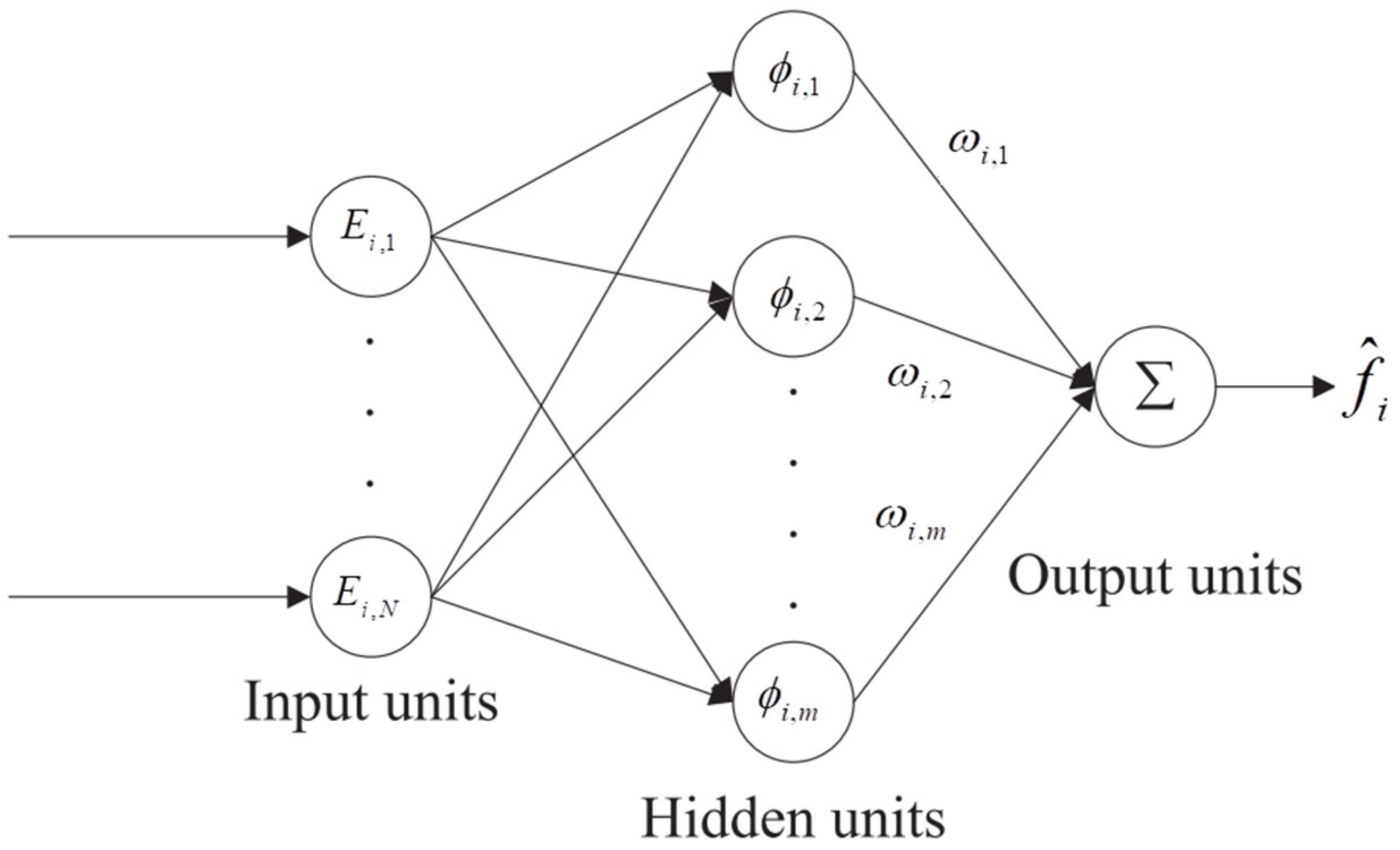
3.3. RBF Neural Network Estimator

RBF neural networks are strong candidates for many uses, such as time series prediction, classification, function approximation, and system control [57,58]. In the current study, the RBF neural network estimates any disturbances and uncertainties, and then its output is used to enhance the performance of the fault-tolerant control. The output of the RBF neural network (${\widehat{f}}_i)$ is calculated as

$${\widehat{f}}_i=f_i^{*}+\epsilon ={\displaystyle \sum }_{j=1}^m{\omega }_{i,j}^{*} {\varphi }_{i,j}\left(E_i\right)+\epsilon =W_i^{*} {\varphi }_i+\epsilon \hspace{1em}\hspace{1em}i=1,2,\dots n_o$$

(14)

$${\varphi }_{i,j}\left(E_i\right)=exp\left(-\frac{{\parallel E_i-c_j\parallel }_2^2}{2b_j^2 }\right)\hspace{1em}\hspace{1em}\hspace{1em}\hspace{1em}j=1,2,\dots ,m,$$

(15)

where the radial basis function’s ideal constant weight is shown by ${\omega }_{i,j}^{*}$, and the number of hidden nodes is represented by $m$. Additionally, $n_o$ denotes the number of outputs, $N$ represents the number of inputs, ${\varphi }_{i,j}$ is the radial basis function of hidden nodes, $\epsilon$ shows the bounded estimation error, $E_i=\left[E_{i,1}, E_{i,2},\dots ,E_{i,N}\right]$ is the input vector of the radial basis function. $b_j$ and $c_j$ indicate the width value and the center of the basis function, respectively [41]. Figure 1 shows the structure of the RBF neural network.

3.4. Problem Formulation

Following the definitions of faults and failures in [59,60,61], their effects on the system can be considered as follows:

$$u_i=u_{ci}+b_i \left(t\right)\left(\left(e_{ii}-1\right)u_{ci}+{\overline{u}}_i\right)\hspace{1em}\hspace{1em}i=1,2, \dots , n$$

(16)

where $u_i$ and $u_{ci}$ denote the actual and desired control input, respectively. Additionally, ${\overline{u}}_i$ is the uncertain fault input. $0 \le e_{ii} \le 1$ represents the effectiveness of the actuator. In addition, $b_i \left(t\right)$ is given by:

$$b_i \left(t \right)=\left\{\begin{array}{cc}0,\hfill & t<t_{0i}\\ 1-e^{-a_i\left(t-t_{0i} \right)}\hfill & t\ge t_{0i}\end{array}\right.$$

(17)

where $a_i>0$ denotes the fault evolution rate; additionally, the time at which the fault occurs is shown by $t_{0i}$. Small and large values of $a_i$ correspond to incipient and abrupt faults, respectively. Using this definition of faults and/or failures results in the following governing equation of the fractional response system:

$$\begin{gathered} D^{q}x=h\left(x\left(t\right),x\left(t-\tau \right)\right)+d+u, \\ u=u_c+\mathit{B} \left(t\right)\left(\left(\mathit{E}-\mathit{I}\right)u_c+\overline{u}\right) \end{gathered}$$

(18)

where $d$ is unknown disturbances and $x={\left[x_1,x_2,\dots ,x_n\right]}^T$, $q={\left[q_1,q_2,\dots ,q_n\right]}^T$ and $d={\left[d_1,d_2,\dots ,d_n\right]}^T$.

Assumption 1.

The bounds of disturbances are assumed to be limited, i.e., there is a positive constant $d_0$ fulfilling $\parallel d\parallel \le d_0$.

Assumption 2.

Since there are limitations on the actuators, control actions and additive fault are constrained, i.e., $\left| u_{ci} \right| \le u_{max}$ and $\left| {\overline{u}}_1 \right|$ ≤ $u_0$.

Let the driving/desired system be as follows:

$$D^{q}y=w\left(y\left(t\right),y\left(t-\tau \right)\right),$$

(19)

where $y={\left[y_1, y_2,\dots ,y_n \right]}^T.$

4. Control Design

Herein, the neural network-based fault-tolerant active control is developed to control and synchronize fractional time-delayed systems. Let us consider the response systems as

$$D_t^{q}x\left(t\right)=h\left(x\left(t\right),x\left(t-\tau \right)\right)+u_c+N_f$$

(20)

where

$$N_f=B \left(t\right)\left( \left( E-I \right)u_c+ \overline{u}\right)+d$$

(21)

Moreover, we define the synchronization error as follows:

$$e=y-x$$

(22)

Defining diagonal matrices $B$ and $B^{\prime }$, respectively, for the response and driving system, we can rewrite the equation of the systems as follows:

$$D_t^{q}x\left(t\right)=B\left(x,t\right)+B^{\prime }\left(x,t-\tau \right)+f\left(x\left(t\right),x\left(t-\tau \right)\right)+N_f+u_c$$

(23)

$$D_t^{q}y\left(t\right)=B\left(y,t\right)+B^{\prime }\left(y,t-\tau \right)+g\left(y\left(t\right),y\left(t-\tau \right)\right)$$

(24)

On the basis of Equations (19) and (20), the nonlinear functions $f\left(x\left(t\right),x\left(t-\tau \right)\right)$ and $g\left(y\left(t\right),y\left(t-\tau \right)\right)$ are as follows:

$$f\left(x\left(t\right),x\left(t-\tau \right)\right)=h\left(x\left(t\right),x\left(t-\tau \right)\right)-B\left(x,t\right)-B^{\prime }\left(x,t-\tau \right)$$

(25)

$$g\left(y\left(t\right),y\left(t-\tau \right)\right)=w\left(y\left(t\right),y\left(t-\tau \right)\right)-B\left(y,t\right)-B^{\prime }\left(y,t-\tau \right)$$

(26)

Based on Equation (22), the error dynamic is given by

$$D_t^{q}e\left(t\right)=Be\left(t\right)+B^{\prime }e\left(t-\tau \right)+g\left(y\left(t\right),y\left(t-\tau \right)\right)-f\left(x\left(t\right),y\left(t-\tau \right)\right)-N_f-u_c$$

(27)

where $e\left(t-\tau \right)=y\left(t-\tau \right)-x\left(t-\tau \right).$ We design the neural network-based fault-tolerant, active control as

$$u_c=-\eta e\left(t\right)-\delta e\left(t-\tau \right)+g\left(y\left(t\right),y\left(t-\tau \right)\right)-f\left(x\left(t\right),y\left(t-\tau \right)\right)-Nsign\left(e\left(t\right)\right)-\widehat{N_f},$$

(28)

where $\eta ={\left[{\eta }_1; {\eta }_2,\cdots ; {\eta }_n\right]}^T$ and $\delta ={\left[{\delta }_1;{\delta }_2,\cdots ; {\delta }_n\right]}^T$ are user-defined parameters that must be selected to satisfy the stability condition of the closed-loop system, which will be given in the following. Additionally, $\widehat{N_f}$ = $\widehat{W}{\varphi }_i$ denotes the estimation of $W^{*}$. The adaptation law is given by

$$\stackrel{·}{{\widehat{W}}_i}=-{\varsigma }_i{e}_i{\varphi }_i$$

(29)

We determine the error of the weight approximation as

$${\tilde{W}}_i= W_i^{*}-{\widehat{W}}_i$$

(30)

where ${\varsigma }_i$ is a used-defined parameter. According to the proposed control, the error dynamic of the synchronization is

$$D_t^{q}e\left(t\right)=Me\left(t\right)+M^{\prime }e\left(t-\tau \right)+Nsign\left(e\left(t\right)\right)+e_d,$$

(31)

where $e_d=\widehat{N_f}-N_f+\epsilon =\widehat{W}{\varphi }_i-W_i^{*}{\varphi }_i+\epsilon$, $\mathrm{M}=B+\eta$ and ${\mathrm{M}}^{\prime }=B^{\prime }+\delta$.

Theorem 3.

Suppose ${\kappa }_{max}$ is the greatest eigenvalue of $M$, $d_{max}=\frac{1}{2}{\parallel M^{\prime }\parallel }_{\infty }$ and $b_{max}=\frac{1}{2}{\parallel M^{\prime }\parallel }_1$. If the user-defined vector $M$ holds the following condition

$$-\left(d_{max}+{\kappa }_{max}\right)>b_{max}>0$$

(32)

as a result, the trajectories of the fractional delayed System (23) will converge to the desired value.

Proof. 

Suppose the following Lyapunov function:

$$V=V_c+\frac{1}{2{\varsigma }_i}{\tilde{W}}_i^2$$

(33)

where $V_c=\frac{1}{2}{e}^T\left(t\right)e\left(t\right)$. The time derivative of the Lyapunov function is as follows:

$$D_t^{q}V=D_t^q{V}_c+\frac{1}{{\varsigma }_i}{D}_t^q{\tilde{W}}_i{\tilde{W}}_i$$

(34)

□

Considering adaption law (29) and Equation (31), we have

$$D_t^{q}V\le D_t^q{V}_c+e_i{\tilde{W}}_i{\varphi }_i=e^T\left(t\right)\left(Me\left(t\right)+M^{\prime }e\left(t-\tau \right)+Nsign\left(e\left(t\right)\right)+\epsilon \right)$$

(35)

Using the RBF neural network, the approximation error ($\epsilon$) is bounded. Based on Lemma 3, we have

$$e^T \left(t\right)M^{\prime }e\left(t-\tau \right)\le d_{max}{e}^T\left(t\right)e\left(t\right)+b_{max}{e}^T \left(t-\tau \right)e\left(t-\tau \right).$$

(36)

By designing parameter $N$ in such a way that $N>\left|\epsilon \right|,$ and substituting Equation (36) to Equation (35), we have

$$\begin{gathered} D_t^{q}V\le e^T\left(t\right)\left(Me\left(t\right)+M^{\prime }e\left(t-\tau \right)\right) \\ \le M{e}^T\left(t\right)e\left(t\right)+d_{max}{e}^T\left(t\right)e\left(t\right)+b_{max}{e}^T \left(t-\tau \right)e\left(t-\tau \right) \\ \le \left(M+d_{max}\right)e^T\left(t\right)e\left(t\right)+b_{max}{e}^T \left(t-\tau \right)e\left(t-\tau \right) \\ \le -R_1{V}_c\left(t\right)+R_2{V}_c\left(t-\tau \right), \end{gathered}$$

(37)

where $R_1=-2\left(M+d_{max}\right)$ and $R_2=2b_{max}$. Now, suppose a linear time-delayed system as follows

$$\left\{\begin{array}{c}{D}_t^{q}w\left(t\right)=-R_{1}w\left(t\right)+R_{2}w\left(t-\tau \right)\\ w\left(t\right)=\varphi \left(t\right)\ge 0,t\in \left[-\tau ,0\right]\end{array}\right.$$

(38)

Following Corollary 1, if the characteristic equation of System (38) does not possess any purely imaginary root, System (27) is asymptotically stable. For Equation (38), the characteristic equation is given by

$$S^q+R_1-R_2{e}^{-s\tau },$$

(39)

Suppose Equation (39) has a purely imaginary root, which is given by

$$s=\omega i=\left|\omega \right|\left(cos\left(\frac{\pi }{2}\right)+i sin\left(\pm \frac{\pi }{2}\right)\right).$$

(40)

Substituting $s=\omega i$ into Equation (40) results in

$${\left(\omega i\right)}^q+R_1-R_2{e}^{-\omega i\tau }=0$$

(41)

Hence, it can be concluded that

$${|{\left(\omega i\right)}^q+R_1|}^2={\left(R_{2}sin\left(\omega \tau \right)\right)}^2+{\left(R_{2}cos\left(\omega \tau \right)\right)}^2$$

(42)

Then, by simple calculation, we have

$${\left|\omega \right|}^{2q}+2R_{1}cos\left(\frac{\alpha \pi }{2}\right){\left|\omega \right|}^q+R_1^2=R_2^2$$

(43)

where $\cos \left(\frac{\alpha \pi }{2}\right)>0, {\left|\omega \right|}^q>0$, and $R_1>0$. If $R_1>R_2$, we can conclude that Equation (39) does not have any real roots. Consequently, the characteristic equation of System (38) will not have any purely imaginary root. Thus, on the basis of Equation (43), Corollary 1, and Lemma 2, the synchronization error (27) becomes zero, and the closed-loop system is asymptotically stable, which wraps up the proof. The pseudocode for the proposed control scheme is presented in Algorithm 1.

Algorithm 1. RBF neural network-based fault-tolerant active control.

For each time step:

1. Receive values of states of driving and response system

2. Calculate the errors of synchronization

3. Update the weights of the RBF neural network based on Equation (29).

4. Calculate the output of neural network ($\widehat{N_f}$) based on Equations (14) and (15) and using the recently obtained wights

5. Calculate the control input based on Equation (28)

6. Apply the obtained control input to the response system

Until the stopping time.

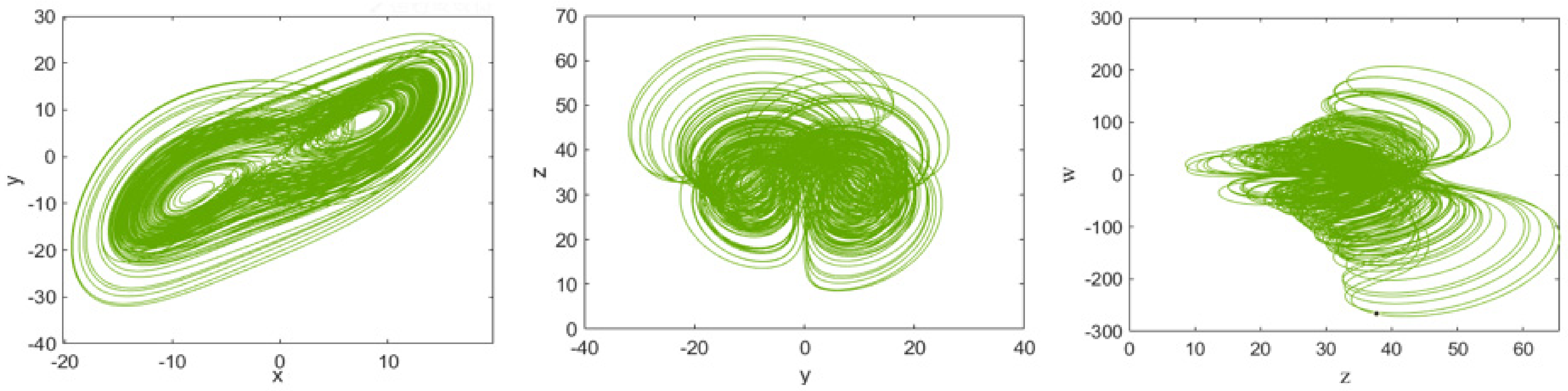
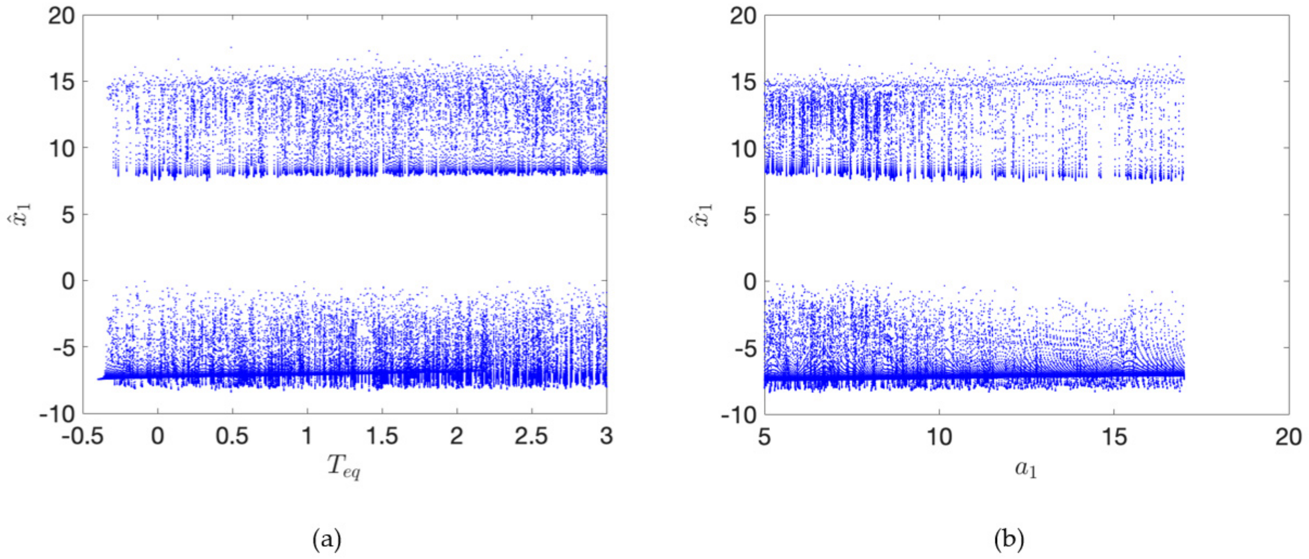
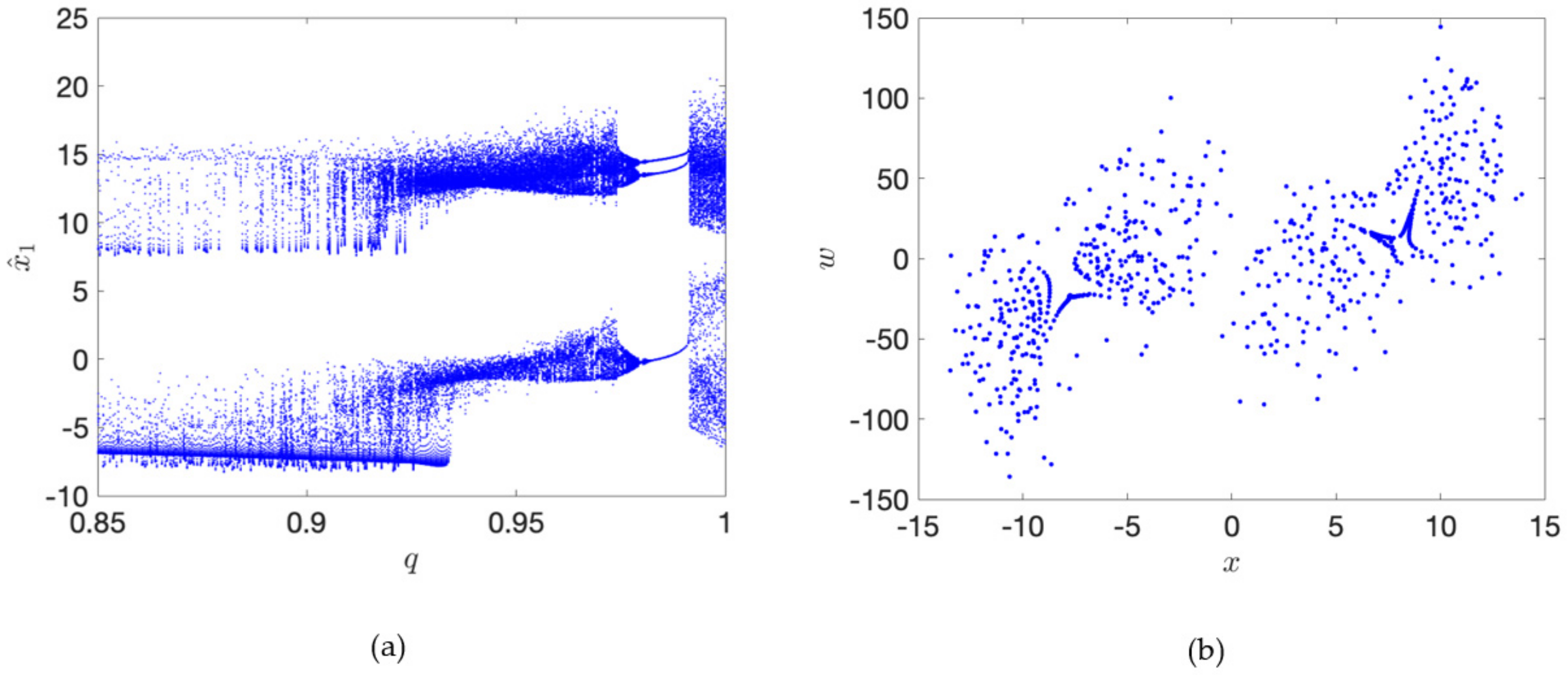
5. Fractional Time-Delayed Memristor System

In [62], a fractional memristor oscillator is presented as

$$\begin{gathered} D^{q}x=a_1\left(y-x\right), \\ {D}^{q}y=a_{2}x-y-xz+a_{3}w-T_{eq}, \\ {D}^{q}z=a_{4}z+xy, \\ {D}^{q}w=a_{5}y+w+a_{6}xM\left(x\right), \end{gathered}$$

(44)

where $0<q<1$ denotes the fractional derivatives. This model is non-dimensional, and consequently, all variables and parameters are dimensionless. Figure 2 displays 2D phase plots of System (44).

Parameter $T_{eq}$ determines the stability conditions of the system, whereas the rest of the parameters are defined as $a_1=10$, $a_2=28$, $a_3=1$, $a_4=-2$, $a_5=27$, and $a_6=-1$, respectively. The Lyapunov exponents for System (44), assuming $T_{eq}=0$, are $L{E}_1=0.667$, $L{E}_2=0.021$, $L{E}_3=0$ and $L{E}_4=-15.517$. The wolf algorithm was considered to compute the Lyapunov spectrum [48]. Figure 3a,b shows the bifurcation diagrams of the fractional System (44) considering a fractional order q = 0.9. The bifurcation diagrams were obtained by plotting the local maxima of state variable $x$ denoted as ${\widehat{x}}_1$. As is evident in Figure 3a, when $-0.5<T_{eq}<3$, chaos is observed. At the same time, chaotic behavior is observed when the parameter $a_1\in \left[5,17\right]$ as shown in Figure 3b. Additionally, in Figure 4a, the bifurcation diagram with respect to the fractional order q is presented. For $0.98<q<0.99,$ a periodic behavior is observed, and then the system gradually reverts to chaos. Additionally, for ($0.84<q<0.98)\cup (0.99<q<1)$ complex behaviors are observed. After that, for $q<0.85,$ the chaotic behavior disappears gradually. Furthermore, the Poincaré map is displayed in Figure 4b considering a plane at $z=30$.

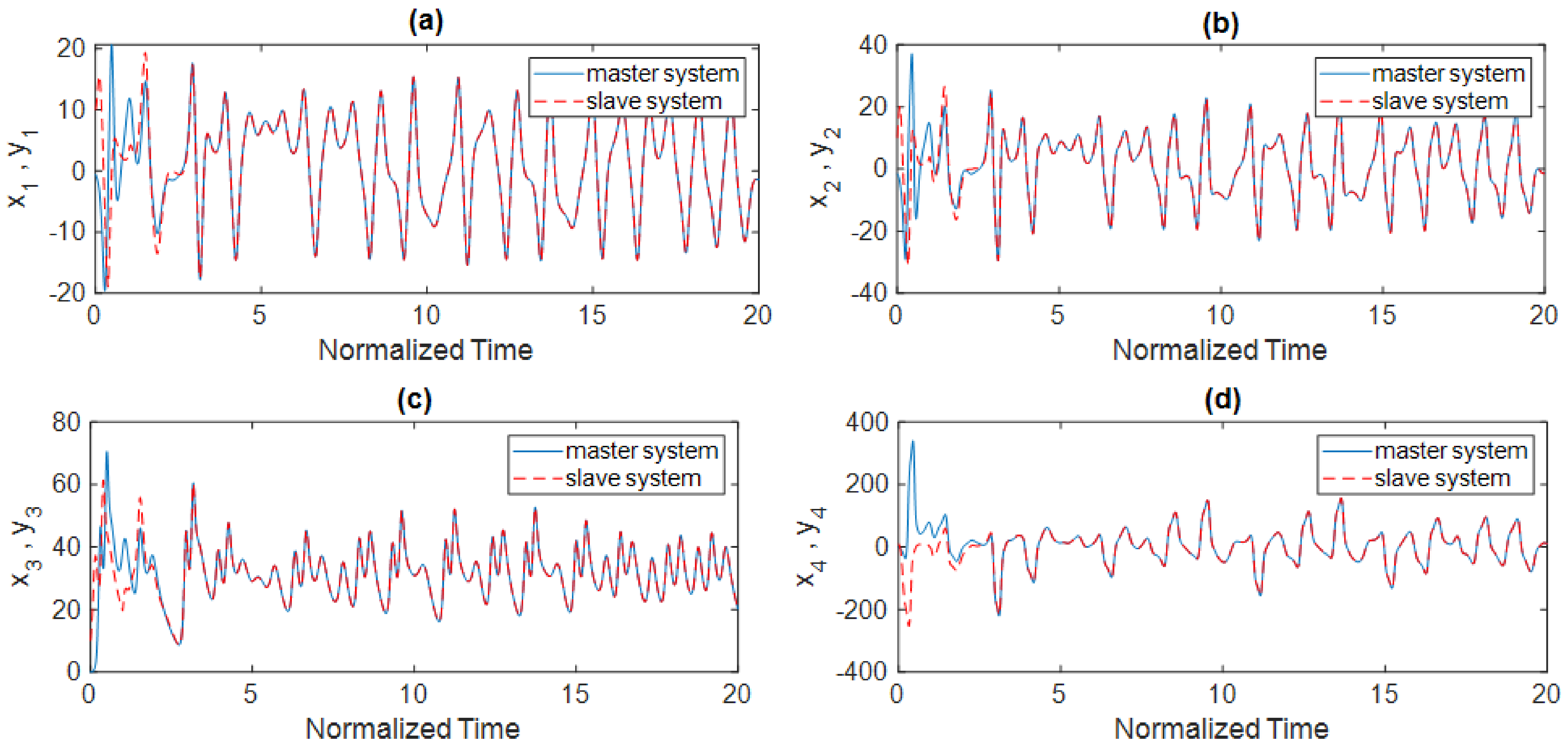
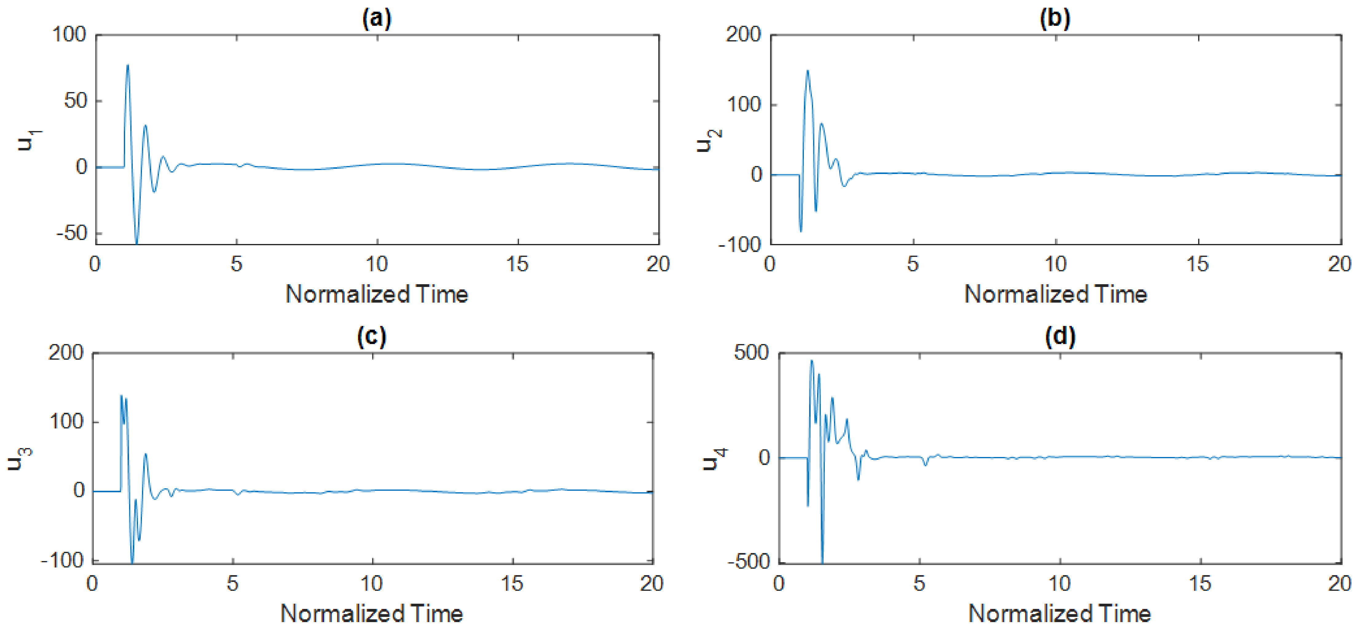
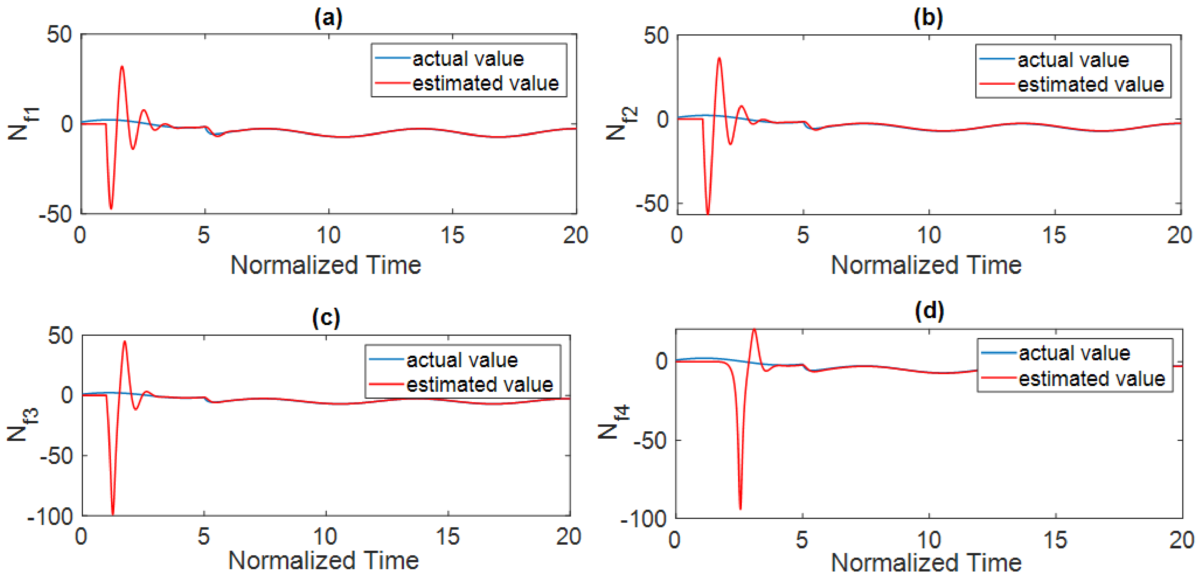
6. Synchronization Results

Now, we consider the fractional time-delayed memristor system with different initial conditions, considered as response and driving systems. Accordingly, the response system in consideration of the control input and the effects of disturbances is given by

$$\begin{gathered} D^q{x}_1=a_1\left(x_2\left(t\right)-x_1\left(t\right)\right)+u_1+d_{x1}, \\ {D}^q{x}_2=a_2{x}_1\left(t\right)-x_2\left(t-\tau \right)-x_1{x}_3\left(t\right)+a_3{x}_4\left(t\right)-T_{eq}+u_2+d_{x2}, \\ {D}^q{x}_3=a_4{x}_3\left(t\right)+x_1\left(t\right)x_2\left(t\right)+u_3+d_{x3}, \\ {D}^q{x}_4=a_5{x}_2\left(t\right)+x_4\left(t-\tau \right)+a_6{x}_1\left(t\right)M\left(x\right)+u_4+d_{x4}. \end{gathered}$$

(45)

Additionally, the driving system is given by

$$\begin{gathered} D^q{y}_1=a_1\left(y_2\left(t\right)-y_1\left(t\right)\right), \\ {D}^q{y}_2=a_2{y}_1\left(t\right)-y_2\left(t-\tau \right)-y_1\left(t\right)y_3\left(t\right)+a_3{y}_4\left(t\right)-T_{eq}, \\ {D}^q{y}_3=a_4{y}_3\left(t\right)+y_1\left(t\right)y_2\left(t\right), \\ {D}^q{y}_4=a_5{y}_2\left(t\right)+y_4\left(t-\tau \right)+a_6{y}_1\left(t\right)M\left(y\right). \end{gathered}$$

(46)

We consider equal values for parameters of both the driving and response system, while the initial conditions of the response and driving system, respectively, are as assumed to be $\left[-5,-1.5, 0,-1.5\right]$ and $\left[10, 10, 10, 10\right]$. The unknown external disturbances are supposed to be

$$d_{x1}\left(t\right)=d_{x2}\left(t\right)=d_{x3}\left(t\right)=d_{x4}\left(t\right)=2\sin \left(t\right)+\cos \left(t\right),$$

(47)

The user-defined parameters of the control scheme are selected as $\eta =\left[1,1,1,1\right], \delta =\left[2,2,2,2\right], N=\left[25,25,25,25\right], {\varsigma }_i=\left[0.01,0.01,0.01,0.01\right].$ The performance of the offered control techniques is evaluated by considering two different kinds of faults, including bias faults, and both bias faults and partial loss of effectiveness which are presented in

Table 1. Parameters of actuator faults.

	Bias Faults Only	Both Bias Faults and Partial Loss of Effectiveness
Actuator control effectiveness ($e_{ii}$)	(1,1,1,1)	(0.8,0.8,0.8,0.8)
Fault evolution rate ($a_i$)	(8,8,8,8)	(12,12,12,12)
Time of occurrence of the fault ($t_{0i}$)	(5,5,5,5)	(5,5,5,5)
Uncertain fault input ($\overline{u}$)	(−5,−5,−5,−5)	(4,4,4,4)

.

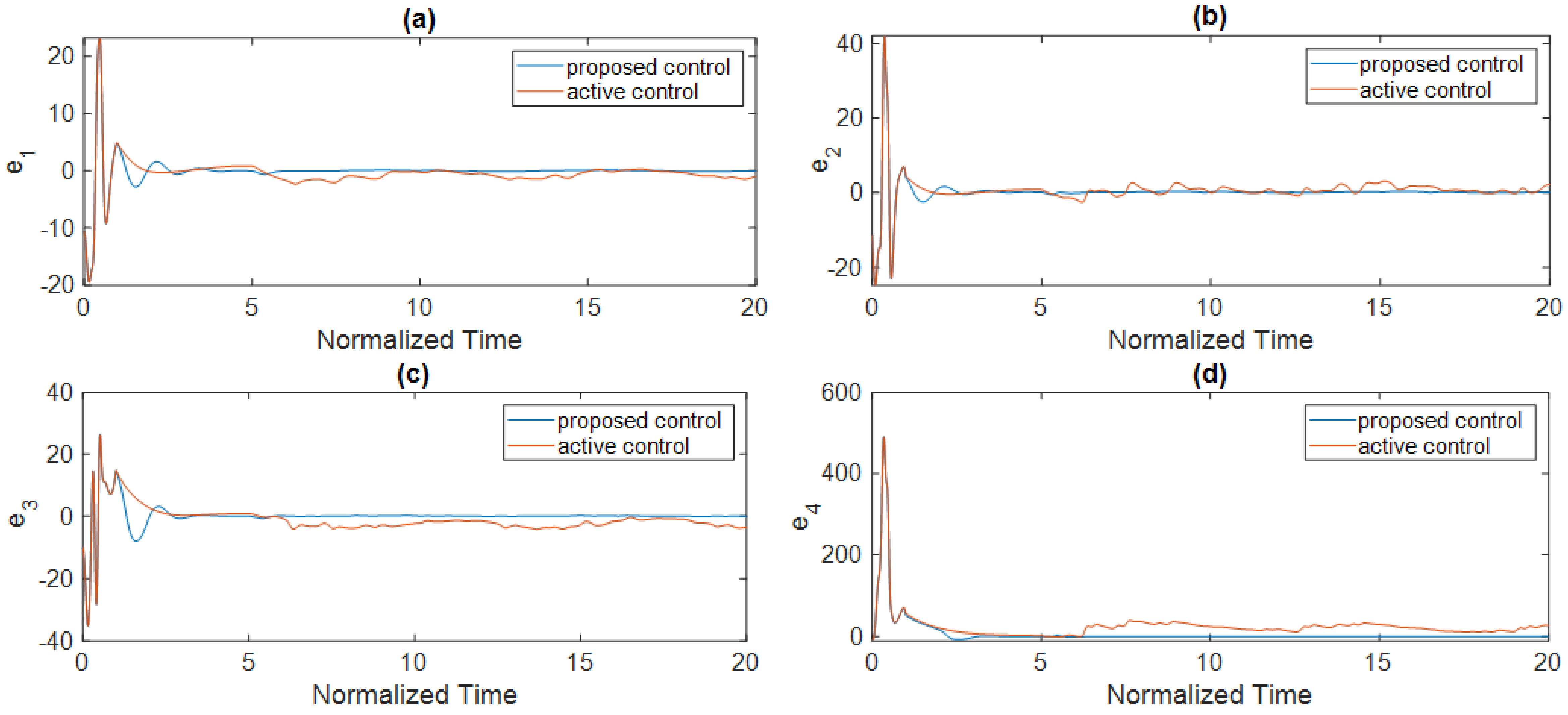
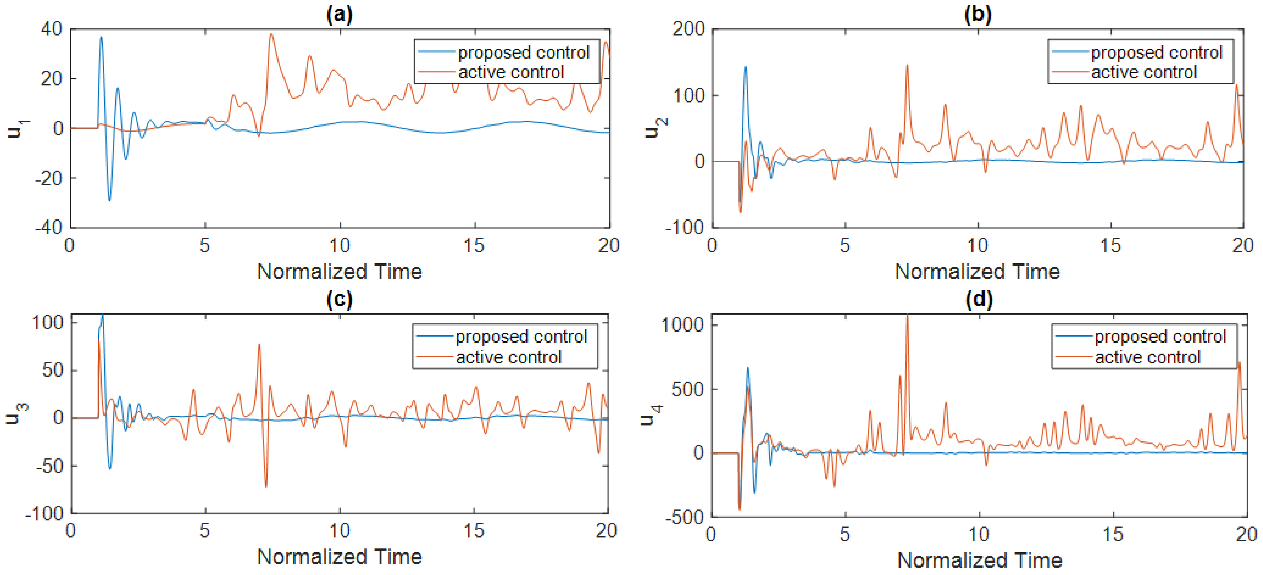
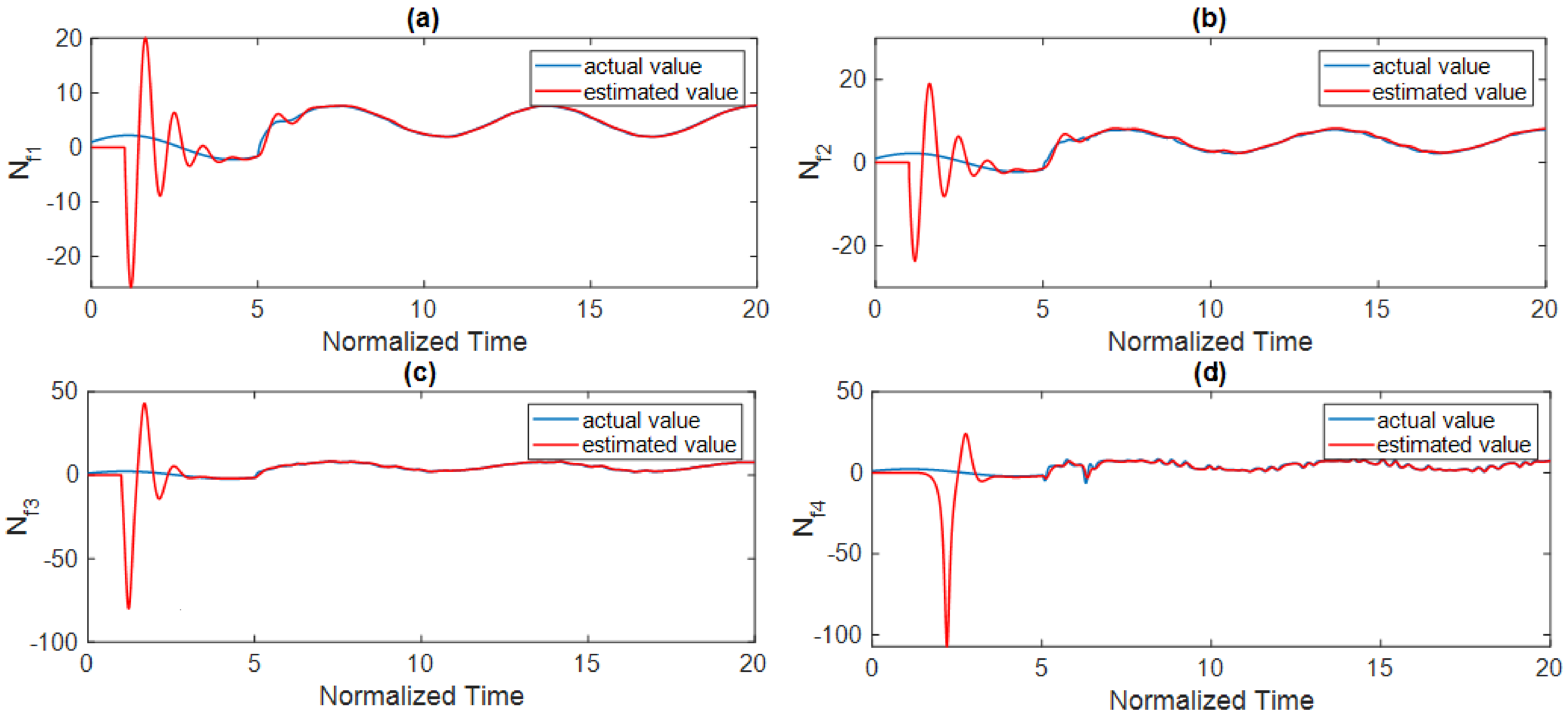
6.1. Synchronization in the Presence of Bias Faults

The controller is turned on at $\mathrm{t}=1,$ and the delay is considered to be $\mathsf{\tau }=1.5$. Figure 5 shows the time-history of synchronization, which clearly shows the offered control method’s effective performance. As illustrated, under the offered methodology, synchronization errors converge to zero over a short time even there are bias faults and unknown disturbances. The control inputs are displayed in Figure 6. As is demonstrated, the amplitudes of control inputs are appropriate. The controller’s appropriate performance in dealing with uncertainties and unexpected faults and failures lies in the precise estimation of the unknown functions achieved by the proposed observer. Figure 7 illustrates the proposed observer’s excellent performance.

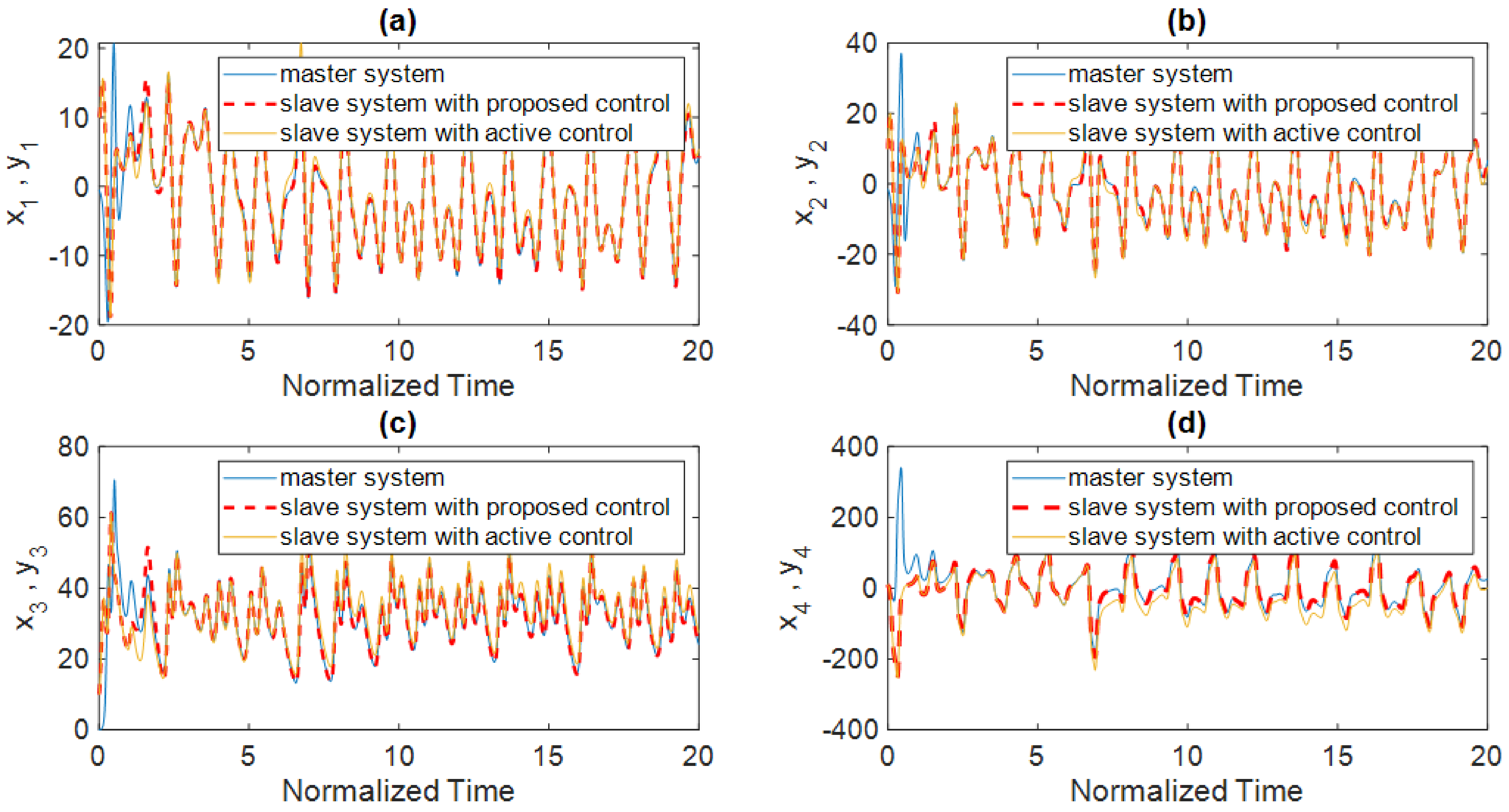
6.2. Comparison and Discussion

To better investigate the performance of the suggested strategy, we compared it with an active control scheme presented by Wang et al. [46]. The parameters of the active control are designed as

$$K=\left[5,5,5,5\right]$$

(48)

For additional information regarding the active control and the factors that ensure the closed-loop system’s stability, see [49].

In this case, the controller is turned on at $t=1$ and $\tau =2,$ and the system is in the presence of both bias faults and partial loss of effectiveness simultaneously. Figure 8 and Figure 9, respectively, show the time history of the synchronization and its error. Additionally, the control inputs are depicted in Figure 10. Finally, in Figure 11, the estimated values of time-varying disturbances and faults that are provided by the proposed technique are presented. By comparing the results of active control with those of the offered controller, it is evident that the suggested technique is faster and more accurate, resulting from the intelligent observer that provides precise information about unknown functions.

Table 2. The norm of synchronization errors and control inputs.

Norm	Proposed Method	Active Control
${\parallel {\mathit{u}}_{{\mathit{x}}_{\mathbf{1}}}\parallel }_{\mathbf{2}}$	113.72	441.83
${\parallel {\mathit{u}}_{{\mathit{x}}_{\mathbf{2}}}\parallel }_{\mathbf{2}}$	522.07	969.81
${\parallel {\mathit{u}}_{{\mathit{x}}_{\mathbf{3}}}\parallel }_{\mathbf{2}}$	346.53	411.23
${\parallel {\mathit{u}}_{{\mathit{x}}_{\mathbf{4}}}\parallel }_{\mathbf{2}}$	2969.43	4775.48
${\parallel {\mathit{e}}_{{\mathit{x}}_{\mathbf{1}}}\parallel }_{\mathbf{2}}$	53.40	100.97
${\parallel {\mathit{e}}_{{\mathit{x}}_{\mathbf{2}}}\parallel }_{\mathbf{2}}$	48.99	115.84
${\parallel {\mathit{e}}_{{\mathit{x}}_{\mathbf{3}}}\parallel }_{\mathbf{2}}$	153.50	287.84
${\parallel {\mathit{e}}_{{\mathit{x}}_{\mathbf{4}}}\parallel }_{\mathbf{2}}$	821.46	2076.86

lists the synchronization errors and control inputs of the suggested technique as well as those of the active control. Table 2 shows that when the suggested technique is used instead of the active controller, the regulation errors are much lower. Table 2 further shows that the values of control inputs for both control systems are in the same order.

On the basis of the simulation results shown in Figure 8, Figure 9, Figure 10 and Figure 11 and Table 2, it can be stated that the suggested technique outperforms active control in terms of accuracy, convergence time, and robustness against faults and disturbances.

The RBF neural network is used in an online platform to detect all unknown functions in the closed-loop system. In this online algorithm, we do not have any data for training and testing. Based only on the adaption rules, the wights of the RBF neural network will be updated. Actually, from the first time step that the controller is turned on, the output of the RBF neural network is used for the controller. Hence, in the beginning, the performance of the RBF neural network is not very good, but after a very short period of time, the RBF neural network learns a structure with an unknown function, and after that, the results are luminous.

It is noteworthy that if we use a very complicated neural network, it may cause overfitting in data which is common in complex neural networks. Hence, we believe RBF neural network, which provides promising results in dealing with unknown functions and is simple compared to other neural networks, is a good choice. However, investigating other types of neural networks for time-delayed fractional-order systems is an appropriate idea for a future study.

7. Conclusions

In this research, the new neural network-based fault-tolerant, active control was proposed for fractional time-delayed systems. Through the neural network estimator, all uncertainties, disturbances, and faults were taken to account. The stability of the offered technique was performed using the active control concept and Lyapunov stability theorem. Then, the fractional memristor system’s dynamical behavior was studied, and the chaotic behavior of the system was illustrated. Finally, the time-delayed system was considered in the presence of different faults, including bias faults and partial loss of effectiveness. By employing the offered control technique, synchronization results of the fractional time-delayed memristor system in the presence of faults and uncertainties were presented. Numerical results confirm the reliability and robustness of the suggested control method for nonlinear time-delayed systems. One of the challenges in the proposed method is the selection of the best user-defined parameters for the controller and neural network. Hence, as a future suggestion, a study can be devoted to the design of a self-tuning mechanism such as evolutionary algorithms and fuzzy self-tuning engines for the proposed control scheme.

References

1. Chen, S.-B.; Rajaee, F.; Yousefpour, A.; Alcaraz, R.; Chu, Y.-M.; Gómez-Aguilar, J.; Bekiros, S.; Aly, A.A.; Jahanshahi, H. Antiretroviral therapy of HIV infection using a novel optimal type-2 fuzzy control strategy. Alex. Eng. J. 2021, 60, 1545–1555. [Google Scholar] [CrossRef]
2. Chen, S.-B.; Beigi, A.; Yousefpour, A.; Rajaee, F.; Jahanshahi, H.; Bekiros, S.; Martinez, R.A.; Chu, Y.-M. Recurrent Neural Network-Based Robust Nonsingular Sliding Mode Control with Input Saturation for a Non-Holonomic Spherical Robot. IEEE Access 2020, 8, 188441–188453. [Google Scholar] [CrossRef]
3. Kosari, A.; Jahanshahi, H.; Razavi, S. An optimal fuzzy PID control approach for docking maneuver of two spacecraft: Orientational motion. Eng. Sci. Technol. Int. J. 2017, 20, 293–309. [Google Scholar] [CrossRef] [Green Version]
4. Xiong, P.-Y.; Jahanshahi, H.; Alcaraz, R.; Chu, Y.-M.; Gómez-Aguilar, J.; Alsaadi, F.E. Spectral Entropy Analysis and Synchronization of a Multi-Stable Fractional-Order Chaotic System using a Novel Neural Network-Based Chattering-Free Sliding Mode Technique. Chaos Solitons Fractals 2021, 144, 110576. [Google Scholar] [CrossRef]
5. Jahanshahi, H.; Sajjadi, S.S.; Bekiros, S.; Aly, A.A. On the development of variable-order fractional hyperchaotic economic system with a nonlinear model predictive controller. Chaos Solitons Fractals 2021, 144, 110698. [Google Scholar] [CrossRef]
6. Li, J.-F.; Jahanshahi, H.; Kacar, S.; Chu, Y.-M.; Gómez-Aguilar, J.; Alotaibi, N.D.; Alharbi, K.H. On the variable-order fractional memristor oscillator: Data security applications and synchronization using a type-2 fuzzy disturbance observer-based robust control. Chaos Solitons Fractals 2021, 145, 110681. [Google Scholar] [CrossRef]
7. Jahanshahi, H.; Bekiros, S.; Gritli, H.; Chu, Y.-M.; Gomez-Aguilar, J.F.; Aly, A.A. Tracking control and stabilization of a fractional financial risk system using novel active finite-time fault-tolerant controls. Fractals 2021. [Google Scholar] [CrossRef]
8. Wang, Y.-L.; Jahanshahi, H.; Bekiros, S.; Bezzina, F.; Chu, Y.-M.; Aly, A.A. Deep recurrent neural networks with finite-time terminal sliding mode control for a chaotic fractional-order financial system with market confidence. Chaos Solitons Fractals 2021, 146, 110881. [Google Scholar] [CrossRef]
9. Bekiros, S.; Jahanshahi, H.; Bezzina, F.; Aly, A.A. A novel fuzzy mixed H2/H∞ optimal controller for hyperchaotic financial systems. Chaos Solitons Fractals 2021, 146, 110878. [Google Scholar] [CrossRef]
10. Wang, H.; Jahanshahi, H.; Wang, M.-K.; Bekiros, S.; Liu, J.; Aly, A. A Caputo–Fabrizio Fractional-Order Model of HIV/AIDS with a Treatment Compartment: Sensitivity Analysis and Optimal Control Strategies. Entropy 2021, 23, 610. [Google Scholar] [CrossRef]
11. Jahanshahi, H. Smooth control of HIV/AIDS infection using a robust adaptive scheme with decoupled sliding mode supervision. Eur. Phys. J. Spéc. Top. 2018, 227, 707–718. [Google Scholar] [CrossRef]
12. Rajagopal, K.; Jahanshahi, H.; Varan, M.; Bayır, I.; Pham, V.-T.; Jafari, S.; Karthikeyan, A. A hyperchaotic memristor oscillator with fuzzy based chaos control and LQR based chaos synchronization. AEU Int. J. Electron. Commun. 2018, 94, 55–68. [Google Scholar] [CrossRef]
13. Jahanshahi, H.; Shahriari-Kahkeshi, M.; Alcaraz, R.; Wang, X.; Singh, V.P.; Pham, V.-T. Entropy Analysis and Neural Network-Based Adaptive Control of a Non-Equilibrium Four-Dimensional Chaotic System with Hidden Attractors. Entropy 2019, 21, 156. [Google Scholar] [CrossRef] [PubMed] [Green Version]
14. Eskandari, B.; Yousefpour, A.; Ayati, M.; Kyyra, J.; Pouresmaeil, E. Finite-Time Disturbance-Observer-Based Integral Terminal Sliding Mode Controller for Three-Phase Synchronous Rectifier. IEEE Access 2020, 8, 152116–152130. [Google Scholar] [CrossRef]
15. Luo, S.; Lewis, F.L.; Song, Y.; Vamvoudakis, K.G. Adaptive backstepping optimal control of a fractional-order chaotic magnetic-field electromechanical transducer. Nonlinear Dyn. 2020, 100, 523–540. [Google Scholar] [CrossRef]
16. Rajagopal, K.; Tuna, M.; Karthikeyan, A.; Koyuncu, I.; Duraisamy, P.; Akgul, A. Dynamical analysis, sliding mode synchronization of a fractional-order memristor Hopfield neural network with parameter uncertainties and its non-fractional-order FPGA implementation. Eur. Phys. J. Spéc. Top. 2019, 228, 2065–2080. [Google Scholar] [CrossRef]
17. Yousefpour, A.; Hosseinloo, A.H.; Yazdi, M.R.H.; Bahrami, A. Disturbance observer–based terminal sliding mode control for effective performance of a nonlinear vibration energy harvester. J. Intell. Mater. Syst. Struct. 2020, 31, 1495–1510. [Google Scholar] [CrossRef]
18. Sabatier, J.; Agrawal, O.P.; Machado, J.A.T. Advances in Fractional Calculus; Springer: Berlin/Heidelberg, Germany, 2007. [Google Scholar]
19. Wang, S.; He, S.; Yousefpour, A.; Jahanshahi, H.; Repnik, R.; Perc, M. Chaos and complexity in a fractional-order financial system with time delays. Chaos Solitons Fractals 2020, 131. [Google Scholar] [CrossRef]
20. Hilfer, R. Applications of Fractional Calculus in Physics; World Scientific: Singapore, 2000. [Google Scholar]
21. Yousefpour, A.; Bahrami, A.; Haeri Yazdi, M.R. Multi-frequency piezomagnetoelastic energy harvesting in the monostable mode. J. Theor. Appl. Vib. Acoust. 2018, 4, 1–18. [Google Scholar]
22. Jahanshahi, H.; Yousefpour, A.; Munoz-Pacheco, J.M.; Moroz, I.; Wei, Z.; Castillo, O. A new multi-stable fractional-order four-dimensional system with self-excited and hidden chaotic attractors: Dynamic analysis and adaptive synchronization using a novel fuzzy adaptive sliding mode control method. Appl. Soft Comput. 2020, 87, 105943. [Google Scholar] [CrossRef]
23. Ladaci, S.; Charef, A. On Fractional Adaptive Control. Nonlinear Dyn. 2006, 43, 365–378. [Google Scholar] [CrossRef]
24. Naik, P.A.; Zu, J.; Owolabi, K.M. Global dynamics of a fractional order model for the transmission of HIV epidemic with optimal control. Chaos Solitons Fractals 2020, 138, 109826. [Google Scholar] [CrossRef]
25. Yousefpour, A.; Jahanshahi, H.; Munoz-Pacheco, J.M.; Bekiros, S.; Wei, Z. A fractional-order hyper-chaotic economic system with transient chaos. Chaos Solitons Fractals 2020, 130, 109400. [Google Scholar] [CrossRef]
26. Wang, S.; Yousefpour, A.; Yusuf, A.; Jahanshahi, H.; Alcaraz, R.; He, S.; Munoz-Pacheco, J.M. Synchronization of a Non-Equilibrium Four-Dimensional Chaotic System Using a Disturbance-Observer-Based Adaptive Terminal Sliding Mode Control Method. Entropy 2020, 22, 271. [Google Scholar] [CrossRef] [Green Version]
27. Romero, O.; Chatterjee, S.; Pequito, S. Fractional-Order Model Predictive Control for Neurophysiological Cyber-Physical Systems: A Case Study using Transcranial Magnetic Stimulation. In Proceedings of the IEEE 2020 American Control Conference (ACC), Denver, CO, USA, 1–3 July 2020; pp. 4996–5001. [Google Scholar]
28. Huang, C.; Cao, J. Active control strategy for synchronization and anti-synchronization of a fractional chaotic financial system. Phys. A Stat. Mech. Appl. 2017, 473, 262–275. [Google Scholar] [CrossRef]
29. Wei, Z.; Yousefpour, A.; Jahanshahi, H.; Kocamaz, U.E.; Moroz, I. Hopf bifurcation and synchronization of a five-dimensional self-exciting homopolar disc dynamo using a new fuzzy disturbance-observer-based terminal sliding mode control. J. Frankl. Inst. 2021, 358, 814–833. [Google Scholar] [CrossRef]
30. Yousefpour, A.; Jahanshahi, H. Fast disturbance-observer-based robust integral terminal sliding mode control of a hyperchaotic memristor oscillator. Eur. Phys. J. Spéc. Top. 2019, 228, 2247–2268. [Google Scholar] [CrossRef]
31. Chen, X.; Komada, S.; Fukuda, T. Design of a nonlinear disturbance observer. IEEE Trans. Ind. Electron. 2000, 47, 429–437. [Google Scholar] [CrossRef]
32. Chen, W.-H.; Yang, J.; Guo, L.; Li, S. Disturbance-Observer-Based Control and Related Methods—An Overview. IEEE Trans. Ind. Electron. 2016, 63, 1083–1095. [Google Scholar] [CrossRef] [Green Version]
33. Xu, B.; Sun, F. Composite Intelligent Learning Control of Strict-Feedback Systems with Disturbance. IEEE Trans. Cybern. 2017, 48, 730–741. [Google Scholar] [CrossRef] [PubMed]
34. Jafari, M.; Xu, H. Intelligent Control for Unmanned Aerial Systems with System Uncertainties and Disturbances Using Artificial Neural Network. Drones 2018, 2, 30. [Google Scholar] [CrossRef] [Green Version]
35. Vahidi-Moghaddam, A.; Rajaei, A.; Vatankhah, R.; Hairi-Yazdi, M.R. Terminal sliding mode control with non-symmetric input saturation for vibration suppression of electrostatically actuated nanobeams in the presence of Casimir force. Appl. Math. Model. 2018, 60, 416–434. [Google Scholar] [CrossRef]
36. Vahidi-Moghaddam, A.; Rajaei, A.; Ayati, M. Disturbance-observer-based fuzzy terminal sliding mode control for MIMO uncertain nonlinear systems. Appl. Math. Model. 2019, 70, 109–127. [Google Scholar] [CrossRef]
37. Yousefpour, A.; Vahidi-Moghaddam, A.; Rajaei, A.; Ayati, M. Stabilization of nonlinear vibrations of carbon nanotubes using observer-based terminal sliding mode control. Trans. Inst. Meas. Control. 2019, 42, 1047–1058. [Google Scholar] [CrossRef]
38. Gao, W.; Selmic, R. Neural network control of a class of nonlinear systems with actuator saturation. Proceed. Am. Control Conf. 2004, 17, 147–156. [Google Scholar] [CrossRef]
39. Chen, M.; Ge, S.S.; How, B.V.E. Robust Adaptive Neural Network Control for a Class of Uncertain MIMO Nonlinear Systems With Input Nonlinearities. IEEE Trans. Neural Netw. 2010, 21, 796–812. [Google Scholar] [CrossRef] [PubMed]
40. Miller, W.T.; Werbos, P.J.; Sutton, R.S. Neural Networks for Control; MIT Press: Cambridge, MA, USA, 1995. [Google Scholar]
41. Liu, J. Radial Basis Function (RBF) Neural Network Control for Mechanical Systems: Design, Analysis and Matlab Simulation; Springer Science & Business Media: Berlin/Heidelberg, Germany, 2013. [Google Scholar]
42. Moradi, M.J.; Roshani, M.M.; Shabani, A.; Kioumarsi, M. Prediction of the Load-Bearing Behavior of SPSW with Rectangular Opening by RBF Network. Appl. Sci. 2020, 10, 1185. [Google Scholar] [CrossRef] [Green Version]
43. Al-Darraji, I.; Piromalis, D.; Kakei, A.; Khan, F.; Stojmenovic, M.; Tsaramirsis, G.; Papageorgas, P. Adaptive Robust Controller Design-Based RBF Neural Network for Aerial Robot Arm Model. Electronics 2021, 10, 831. [Google Scholar] [CrossRef]
44. Roshani, M.; Phan, G.T.; Ali, P.J.M.; Roshani, G.H.; Hanus, R.; Duong, T.; Corniani, E.; Nazemi, E.; Kalmoun, E.M. Evaluation of flow pattern recognition and void fraction measurement in two phase flow independent of oil pipeline’s scale layer thickness. Alex. Eng. J. 2021, 60, 1955–1966. [Google Scholar] [CrossRef]
45. Ma, W.; Chen, Z.; Zhu, Q. Ultra-Short-Term Forecasting of Photo-Voltaic Power via RBF Neural Network. Electronics 2020, 9, 1717. [Google Scholar] [CrossRef]
46. Wang, S.; Yu, Y.; Wen, G. Hybrid projective synchronization of time-delayed fractional order chaotic systems. Nonlinear Anal. Hybrid Syst. 2014, 11, 129–138. [Google Scholar] [CrossRef]
47. Gao, Z.; Yan, M.; Wei, J. Robust stabilizing regions of fractional-order PDμ controllers of time-delay fractional-order systems. J. Process. Control. 2014, 24, 37–47. [Google Scholar] [CrossRef]
48. Liu, H.; Yang, J. Sliding-Mode Synchronization Control for Uncertain Fractional-Order Chaotic Systems with Time Delay. Entropy 2015, 17, 4202–4214. [Google Scholar] [CrossRef] [Green Version]
49. Behinfaraz, R.; Badamchizadeh, M.A.; Ghiasi, A.R. An approach to achieve modified projective synchronization between different types of fractional-order chaotic systems with time-varying delays. Chaos Solitons Fractals 2015, 78, 95–106. [Google Scholar] [CrossRef]
50. Li, C.; Deng, W. Remarks on fractional derivatives. Appl. Math. Comput. 2007, 187, 777–784. [Google Scholar] [CrossRef]
51. Deng, W.; Li, C.; Lü, J. Stability analysis of linear fractional differential system with multiple time delays. Nonlinear Dyn. 2007, 48, 409–416. [Google Scholar] [CrossRef]
52. Zhang, W.; Cao, J.; Wu, R.; Alsaadi, F.E.; Alsaedi, A. Lag projective synchronization of fractional-order delayed chaotic systems. J. Frankl. Inst. 2019, 356, 1522–1534. [Google Scholar] [CrossRef]
53. Li, Y.; Chen, Y.; Podlubny, I. Stability of fractional-order nonlinear dynamic systems: Lyapunov direct method and generalized Mittag–Leffler stability. Comput. Math. Appl. 2010, 59, 1810–1821. [Google Scholar] [CrossRef] [Green Version]
54. Li, Y.; Chen, Y.; Podlubny, I. Mittag–Leffler stability of fractional order nonlinear dynamic systems. Automatica 2009, 45, 1965–1969. [Google Scholar] [CrossRef]
55. Aguila-Camacho, N.; Duarte-Mermoud, M.A.; Gallegos, J.A. Lyapunov functions for fractional order systems. Commun. Nonlinear Sci. Numer. Simul. 2014, 19, 2951–2957. [Google Scholar] [CrossRef]
56. Zhang, W.; Cao, J.; Wu, R.; Alsaedi, A.; Alsaadi, F.E. Projective synchronization of fractional-order delayed neural networks based on the comparison principle. Adv. Differ. Equ. 2018, 2018, 73. [Google Scholar] [CrossRef] [Green Version]
57. Seshagiri, S.; Khalil, H. Output feedback control of nonlinear systems using RBF neural networks. IEEE Trans. Neural Netw. 2000, 11, 69–79. [Google Scholar] [CrossRef] [PubMed] [Green Version]
58. Akbilgic, O.; Bozdogan, H.; Balaban, M.E. A novel Hybrid RBF Neural Networks model as a forecaster. Stat. Comput. 2014, 24, 365–375. [Google Scholar] [CrossRef]
59. Jin, X. Fault tolerant finite-time leader–follower formation control for autonomous surface vessels with LOS range and angle constraints. Automatica 2016, 68, 228–236. [Google Scholar] [CrossRef]
60. Murugesan, S.; Goel, P.S. Fault-tolerant spacecraft attitude control system. Sadhana 1987, 11, 233–261. [Google Scholar] [CrossRef]
61. Zuo, Z.; Ho, D.W.; Wang, Y. Fault tolerant control for singular systems with actuator saturation and nonlinear perturbation. Autom. 2010, 46, 569–576. [Google Scholar] [CrossRef]
62. Jahanshahi, H.; Yousefpour, A.; Munoz-Pacheco, J.M.; Kacar, S.; Pham, V.-T.; Alsaadi, F.E. A new fractional-order hyperchaotic memristor oscillator: Dynamic analysis, robust adaptive synchronization, and its application to voice encryption. Appl. Math. Comput. 2020, 383, 125310. [Google Scholar] [CrossRef]
Figure 1. The scheme of the RBF neural network.
Electronics 10 01501 g001
Figure 2. Phase plots of the fractional memristor system with q = 0.97 .
Electronics 10 01501 g002
Figure 3. Bifurcations diagrams of System (44) with q = 0.9 . (a) for T e q with a 1 = 10 , (b) for a 1 with T e q = 0 .
Electronics 10 01501 g003
Figure 4. (a) Bifurcations diagrams of System (44) for q with T e q = 0 , and a 1 = 10 . (b) Poincaré section on x w plane at z = 30 .
Electronics 10 01501 g004
Figure 5. Synchronization results based on the offered control methodology where there are bias faults. Time history of (a) x_1 and y_1, (b) x_2 and y_2, (c) x_3 and y_3, (d) x_4 and y_4.
Electronics 10 01501 g005
Figure 6. The control input based on the offered control methodology where there are bias faults. Time history of (a) u_1, (b) u_2, (c) u_3, (d) u_4.
Electronics 10 01501 g006
Figure 7. Estimated and actual values of faults and disturbances where there are bias faults. Disturbances and faults that are imposed on (a) x_1, (b) x_2, (c) x_3, (d) x_4.
Electronics 10 01501 g007
Figure 8. Synchronization results based on the proposed control methodology and active control, where there are both bias faults and partial loss of effectiveness. Time history of states (a) x 1 and y 1 , (b) x 2 and y 2 , (c) x 3 and y 3 , (d) x 4 and y 4 .
Electronics 10 01501 g008
Figure 9. The error of synchronization based on the proposed control methodology and active control, where there are both bias faults and partial loss of effectiveness. Time history of (a) e 1 , (b) e 2 , (c) e 3 , (d) e 4 .
Electronics 10 01501 g009
Figure 10. The control input based on the proposed control methodology and active control, where there are both bias faults and partial loss of effectiveness. Time history of (a) u 1 , (b) u 2 , (c) u 3 , (d) u 4 .
Electronics 10 01501 g010
Figure 11. Estimated and actual value of faults and disturbances, where there are bias faults and partial loss of effectiveness. Disturbances and faults that are imposed on (a) x 1 , (b) x 2 , (c) x 3 , (d) x 4 .
Electronics 10 01501 g011