Article

Sentiment Analysis of before and after Elections: Twitter Data of U.S. Election 2020

1
Dipartimento di Elettronica, Informazione e Bioingegneria (DEIB), Politecnico di Milano, 20133 Milano, Italy
2
Department of Computer and Information Sciences, CCIS, Prince Sultan University, Riyadh 66833, Saudi Arabia
3
Department of Telecommunication Engineering, University of Engineering and Technology Taxila, Taxila 47080, Pakistan
4
Department of Computer Engineering, University of Engineering and Technology Taxila, Taxila 47080, Pakistan
5
Department of Computer Science, University of Gujrat, Gujrat 50781, Pakistan
6
Department of Computer Sciences, Quaid-i-Azam University, Islamabad 45320, Pakistan
*
Authors to whom correspondence should be addressed.
Electronics 2021, 10(17), 2082; https://doi.org/10.3390/electronics10172082
Submission received: 29 July 2021 / Revised: 20 August 2021 / Accepted: 24 August 2021 / Published: 27 August 2021
(This article belongs to the Special Issue Machine Learning Technologies for Big Data Analytics)

Abstract

:
U.S. President Joe Biden took his oath after being victorious in the controversial U.S. elections of 2020. The polls were conducted over postal ballot due to the coronavirus pandemic following delays of the announcement of the election’s results. Donald J. Trump claimed that there was potential rigging against him and refused to accept the results of the polls. The sentiment analysis captures the opinions of the masses over social media for global events. In this work, we analyzed Twitter sentiment to determine public views before, during, and after elections and compared them with actual election results. We also compared opinions from the 2016 election in which Donald J. Trump was victorious with the 2020 election. We created a dataset using tweets’ API, pre-processed the data, extracted the right features using TF-IDF, and applied the Naive Bayes Classifier to obtain public opinions. As a result, we identified outliers, analyzed controversial and swing states, and cross-validated election results against sentiments expressed over social media. The results reveal that the election outcomes coincide with the sentiment expressed on social media in most cases. The pre and post-election sentiment analysis results demonstrate the sentimental drift in outliers. Our sentiment classifier shows an accuracy of 94.58% and a precision of 93.19%.

1. Introduction

The U.S. election, 2020 was a significant global event, as the Republican Party’s Donald Trump was striving to secure his second term while Joe Biden of the Democratic Party expected to turn it around. The pre-election polls assessed the U.S. public’s sentiments to evaluate the likelihoods for each candidate. The BBC poll suggested that Joe Biden was ahead of Donald Trump and marked the elections’ battleground [1]. However, among these states, the margin of victory was very close, and it could have swung in favor of either candidate. Other two-way and four-way online polls such as 270 to win and Real clear politics showed the narrow dominance of Joe Biden. The nationwide polls such as Ipsos/Reuters [2], CNBC, Yahoo News [3], NBC/WSJ [4], Fox News [5], CNN/WSJ [6], ABC/Washington Post [7], and others reported public sentiment in favor of Joe Biden. However, since U.S. elections are decided by the Electoral College rather than on casted votes, predicting elections on public sentiment is not straightforward. It might reflect the public opinion in one sense; however, it could sway in favor of any candidate with such a narrow margin. The 2020 U.S. election took place on 3 November 2020; the final results of the election declared Joe Biden victorious with 51.3%, while Donald Trump bagged 46.9% votes. The 2020 U.S. election was the first election after 1992 in which the incumbent president was unable to retain his seat. The election of 2020 also witnessed one of the highest voter turnouts since 1900, in which both candidates received more than 74 million votes [8].
The elections were held during the COVID-19 pandemic in the U.S.; therefore, strict SOPs and stay-at-home instructions were enforced. The pandemic affected and altered the elections campaigns and schedules and resulted in long queues at election booths due to reduced numbers of workers willing to work during a pandemic. This paved the way for mail-in voting and casting of the vote through postage. Donald Trump criticized the mail-in poll by stating that it raised the chances of fraud and rigging. Since many votes were cast by postage, the compilation of the results witnessed a delay. The delay in the result announcement allowed Donald Trump to issue several statements about rigging and stealing the mandate of the people of the U.S. However, the delay in result also happened during the U.S. election in 2000, which took 36 days, and Al Gore lost with a narrow margin. After the elections, Trump refused to have a peaceful transition of power, stating that the only way he could have potentially lost the elections was through fraud. The case of the election of 2000 was contested in the U.S. Supreme Court, where the court initially ruled for a recounting of votes in the disputed Florida state. Later, the decision was withheld to avoid inconsistent standards of counting in different U.S states. Immediately after the 2020 election, Donald Trump threatened lawsuits and dubbed the election as fraudulent. However, his legal battle suffered initial blows when Attorney General William Barr turned it down by saying, “To date, we have not seen fraud on a scale that could have effected a different outcome in the election”. The federal court of Pennsylvania also ruled against him, to quote the Judge, “Charges of unfairness are serious. But calling an election unfair does not make it so. Charges require specific allegations and then proof. We have neither here”. Nevertheless, the margin of victory in the 2020 elections was much more prominent compared to 2000.
Social media platforms such as Twitter, Instagram, and Facebook are common ways of expressing sentiments. People share news, discuss political events and comment about certain global happenings. Therefore, social media is used in political campaigns, promoting social and development works, and expressing sentiments about elections. One of the earliest cases of social media usage for a political campaign was during the U.S. election 2008. Barack Obama utilized Twitter for his political campaign to significant effect. One of the recent examples is the U.S. elections of 2016, where the victory of Donald Trump over Hillary Clinton shocked everyone. The pre-election polls suggested Hillary’s dominance over his counterpart with 91.5% in her favor (Real Clear Politics, 2017; Business Insider, 2016). After Trump’s victory, several investigations reveal the role social media played in the elections. Even Trump dubbed it a critical tool that played a pivotal role in his victory (CBS, 2016). Several works on the sentiment analysis of U.S. elections have already been carried out: of the 2012 U.S. election, employing the Naive Bayes Classifier using Unigram features [9], the 2016 U.S. election, employing the lexicon approach [10], the 2016 U.S. elections using Sentistrenght [11] and other elections, such as Indian elections [12,13], Iranian elections [14], Singaporean elections [15], and Colombian elections [16]. These works provide insights into social media sentiments as well as their correspondence with the actual election results; further details are provided in Section 2. Similarly, social media analysis of the 2020 U.S. election can also potentially unveil several hidden sentiments about both candidates. The study can become yet more critical since the shadows of rigging are cast on the elections. The sentiment analysis becomes more interesting since votes were cast via postal services.
The sentiment analysis of elections also has limitations; for example, it is hard to recognize sarcasm trivially. In some cases, the negative sentiments are classified as positive due to their writing styles. Generally speaking, Twitter is a much better place for sentiment analysis as compared to Facebook [17]. In this sense, some people on social media might not be serious in really expressing their actual feelings. Therefore, their sentiments do not reflect the true picture. Moreover, social media might not represent complete sentiment in elections, since all voters are not present. While social media might not represent everyone completely, it provides a sample space of people’s opinions. Also, some people might not want to reveal their views due to privacy issues, so even if they are on social media, they might not express their true opinion [18]. Nevertheless, despite all these limitations, social media sentiment analysis provides the nearest approximation of public sentiment. To detect sarcasm, we used bigram along with term frequency and inverse document frequency (TF-IDF). Bigram is effective for sarcasm detection since it takes into account words surrounding a specific term considering the context along with the single word itself; further details are provided in Section 3.2.
This research investigates pre- and post-election sentiments for both candidates in each state. Outliers are well known in fundamental data mining tasks to find extreme values laying outside the trends followed by other data samples [19,20]. Since the U.S. has flip and closely contested states, finding the outliers is significant for data analysis. Moreover, we analyzed public sentiment and compared it with the election results state-wise. To the best of our knowledge, we have not seen any comprehensive analysis of the 2020 U.S. election that covered pre- and post-election scenarios and compared them with previous U.S. elections. To summarize, the contributions of the work are:
1.
We formulated a dataset for the 2020 U.S. election before, during, and after elections using Tweepy API. We created a unique dataset comprising pre and post-election tweets;
2.
In this work, we employed sentiment analysis over the Twitter dataset and compared it with the the 2020 U.S. election results;
3.
The state with strong and weak sentiments for Donald Trump and Joe Biden were analyzed. We identified outliners and analyzed swing states;
4.
We analyzed pre- and post-election sentiments and investigated sentiment drift before, during, and after elections;
5.
We assessed the shift of opinions in states with narrow margins and flip states;
6.
We compared the the 2020 U.S. election sentiments with the U.S. election 2016 and identified the mutations in various states;
7.
We highlighted the critical agenda and issues based on which voters cast their votes.
The remainder of this paper is organized as follows. Section 2 discusses state of art and existing work in this field. Section 3 discusses proposed techniques and algorithms used for sentiment analysis. Section 4 presents the results of simulations performed over the Twitter dataset. Finally, Section 6 illustrates the conclusion of the work.

2. Related Work

Sentiment analysis is defined as a process that automates the mining of attitudes, opinions, views, and emotions from text, speech, tweets, and database sources through Natural Language Processing (NLP) [21]. Sentiment analysis involves classifying opinions in text into three main categories, i.e., “positive” or “negative” or “neutral” [22]. Sentiment information can be extracted using various ways, including speaker recognition [23], physical activity recognition [24], philological signals [25], human facial features [26], and textual information expressed over social media. Sentiment analysis is employed in numerous fields for opinion mining, such as focusing on multi-level single and multi-word aspects to manifest several domains in Twitter datasets [27], in recommendation systems [28], being employed for business intelligence [29], for finding public opinion about a particular rule before presentation (“eRuleMaking”) [30], in comments analysis [31], News Sentiment Analysis [32], movie reviews analysis [33], for analysing the sensitivity of particular content before publishing or advertising [34], or to determine public opinion before elections in different countries. Elections are a significant component for any democratic country which involves the expression of opinion using a vote. People also express their opinions on social media regarding elections. For example, this was seen in the U.S. regarding the presidential election in 2020 [35,36], in India [12,13,37], in Australia [38], in the 2013 Pakistani elections and 2014 Indian elections [39], in Nigeria [40], in the Punjab Legislative Assembly [41], in Indonesia [42], in the 2013 Pakistan elections 2013 [43], in Indonesia [44], in Iran [14], in the Colombian election in 2014 [16] and in the Singaporean election in 2011 [15]. Researchers use several techniques and approaches for text classification task in sentiment analysis [45]. In particular, three main types of conventional approaches for the text classification are used in sentiment analysis, named: lexicon-based approaches, machine learning approaches and the fusion of the prior-mentioned two approaches, named hybrid approaches [27].
The 2020 U.S. election is controversial since allegations of rigging and result manipulations surround it. The sentiment analysis reveals several hidden aspects of public opinion for different parties and candidates and would unleash similar sentiments for a given state. In the literature, various aspects of elections are analyzed using sentiment analysis. U.S. elections are one of the most observed international events, as they affect and influence different countries’ policy-making approaches and economies. Sentiment analyses are published in several works for previous elections. In [9], the author proposed a system providing analysis of public sentiment toward presidential candidates in the 2012 U.S. election by using the Naive Bayes classifier for sentiment analysis on unigram features. They calculated features from tweets tokenization to preserve the punctuation and extract intact URLs for the significance of sentiment. Their system obtained 59% accuracy in classification for four categories of sentiment. Their system was not strictly motivated for global accuracy as they obtained results for four categories on a specific range. In another research work [11], the author proposed a model for the analysis of political homophily among Twitter users during the 2016 American presidential election. They defined six user classes regarding their sentiment towards Donald Trump and Hillary Clinton. The research reported that if there are reciprocal connections, multiplexed connections, or similar speeches, then the homophily level increases. They used the SentiStrength tool that works on a lexicon-based approach using the dictionary method to perform sentiment analysis. Further, they applied the LDA algorithm to find the hot topic of each user and then aggregated those words to catch the most repeated words. In the mentioned paper [46], during the U.S. presidential elections that took place in November 2016, the author explored the elements of the political discussion that took place on Twitter. They focused on specific user attributes such as frequently mentioned and highlighted terms, the number of followers and friends, etc. For this purpose, a model based on user behavior was developed to identify the basic characteristics of the political negotiation of Twitter and to test several hypotheses. Further, they used the SentiStrength tool to score the sentiments, and they fed their data into the SQL database for exploratory analysis by focusing on retweets and # tags for feature extraction. The obtained results disclosed that the sentiment of the tweets was negative for the top election candidates. In another work [10], the author considered the 2016 U.S. presidential election by analyzing tweets using the lexicon-based approach to regulate the fundamental objects of public sentiments. They discovered the subjectivity measures and positive/negative polarity for understanding the user opinion in the mentioned paper. They used APIs for text preprocessing and proposed an algorithm to calculate the subjectivity measures and polarity scores. In addition, the type of sentiment comparison was made, and the most regularly used words in the tweets were the main effect in plotting a word cloud.
In another research work [47], the author proposed an approach to check shared correlation by comparing the calculated sentiment of tweets with the polling data. For this purpose, they used a lexicon and the Naive Bayes algorithm to quantify and classify all the political tweets collected before the election by considering automatically and manually labeled tweets for this calculation. They came up with a high correlation of 94% with the moving average smoothing technique by concentrating on the tweets 43 days before the election. In another research paper [48], the author considered the tweets of the 2016 U.S. presidential election. They developed a sentiment algorithm that involved some significant functions to scan the tweets for multiple hashtags, noticed the main discussion topics, assigned a particular value to each word, and identified negation words. Furthermore, they also focused on finding the geographical location effects on each candidate’s popularity and the state population ratio and analyzed the most prevalent issues in tweets. They compared their results with the Electoral Collage and found that the sentiments of tweets coincide with the actual outcome by 66.7%. In another research work [49], the author investigated a problem related to spatio-temporal sentiment analysis through a major project in the field of data science. They adopted a semi-supervised approach to observe the exact political disposition and LDA algorithm to find politics-related keywords. They used an unsupervised method, word2vec, to set the selected words into a tight semantic margin. They used a compass classification model that uses a linear classifier such as an SVM, which works as two classifiers for classifying tweets, first classifying a particular tweet into non-political or political and the second to observe the political aligning. The main objective of their work was to keep track of arbitrary temporal intervals based on geo-tagged tweets collected for the U.S. presidential election. By combining data management and machine learning techniques, they achieved satisfactory results, and their approach was also capable of influencing other social issues such as health indicators.
In another work [50], the author proposed the study of the U.S. presidential election held on 3 November 2020 by releasing a dataset consisting of 1.2 billion tweets by tracking all the events and political trends from 2019 and onwards. Their main focus was on the Democratic primaries, Republican and presidential contenders’ real-time tracking. They used a dataset that focused on presidential elections, vice-presidential candidates, presidential candidates, and the wave of transition to the Biden ministry from the Trump ministry. In the mentioned paper [51], the author worked on the dataset provided by Kaggle, which was updated on 18 November 2020, to find sentimental tweets for both top presidential candidates by considering two case studies. Their objectives included the evaluation of location-based tweets and the on-ground opinion of the public regarding the election results. They compared two models: Firstly, VADER (Valence Aware Dictionary for Sentiment Reasoning) depicts emotional severity by portraying the linguistic aspects. Secondly, exploratory data analysis assists in grasping the content of data. In particular, they acquired all the spatial features from the user location using OpenCage API. They then conducted sentiment analysis using VADER that worked for the polarity and severity of emotion used in the text. Finally, they found that positive/negative sentiments were outweighed by neutral sentiments. The author addressed the possible challenges of sentiment analysis for dynamic events in elections in [52], such as a fast-paced change in the datasets, candidate dependence, identifying user’s political preferences, content-related challenges, e.g., hashtags, sarcasm, and links. They also considered interpretation-related challenges such as sentiment versus emotion analysis, vote versus engagement counting, trustworthiness-related challenges, and the importance of location.

3. System Model and Proposed Technique

Our proposed method consists of three main steps, which include: data retrieval and pre-processing, feature extraction, and sentiment analysis, as shown in Figure 1. After data were retrieved, they were filtered to remove content not useful in sentiment analysis, such as links, URLs, retweets, usernames, stopwords, and emoticons. The data were clustered into five zones to find region-wise sentiments. After tokenization and pre-processing, features were extracted using term frequency, inverse document frequency (TF-IDF), bigrams, and trigrams. Finally, Naive Bayes was employed to classify sentiments, as explained in the subsequent sections.

3.1. Data Retrieval and Pre-Processing

A total of 38,432,811 tweets were collected, employing streaming Tweepy API across the United States between 28 September 2020, and 20 November 2020. Since location was crucial to determine the state, tweets without location were filtered. There might have been spamming or bulk twittering by political activists for narrative shaping. We considered the top five tweets per user per day; after filtering the remaining 18,432,811 tweets, we employed sentiment analysis. The collected tweets were generally between 50 and 100 words, while some tweets also lay in the range of 100 and 150 words, as shown in Figure 2. Although the Geotagging of tweets was feasible, undisclosed locations could also be determined by utilizing IP addresses [44]. However, due to virtual private networks (VPNs), this location might not be accurate [49]. Since the location was critical in our analysis, this study filtered out undisclosed locations. For prediction, all the extracted data were arranged based on geolocations.
The purpose of the pre-processing module is to perform the filtration process that uses python libraries to retrieve the most important and meaningful parts of the tweets by excluding the unnecessary content. Unprocessed data fetched from any source are usually in raw form and contain several irrelevant attributes, e.g., links, URLs, retweets, usernames, stopwords, emoticons, etc. used in the process of the classification of Twitter data in the context of elections. The tweets are required to be pre-processed accordingly before analysis by removing all the irrelevant attributes from the dataset to avoid any contradiction of the results [48]. Text pre-processing comprises several steps, including data cleansing that includes excluding unrelated data in terms of stop words, slang, URLs, smilies, irrelevant and redundant data. We mainly used five steps to pre-process the data, including tokenization, stopwords, slang elimination, unique character extraction, and URL removal. In particular, we carried out the removal of missing geolocation tweets and lastly, state-wise data separation, as shown in Figure 3.

3.2. Feature Extraction

TF-IDF is a well-known technique in Natural Language Processing (NLP) for obtaining useful words and their scores from the given corpus [53]. TF represents how many times a particular word has appeared in the corpus. Another significant measure of the importance of a word is document frequency (DF); it describes how many documents contain a specific term. IDF is the multiplicative inverse of DF; along with TF, it provides a measure of the occurrence of certain words. The term frequency t f ( i , δ ) is given in Equation (1):
t f ( i , δ ) = f δ ( i ) m a x w d f δ ( w )
where f δ ( i ) is the term frequency of i in the document δ , while f δ ( w ) is the total words in document δ . Similarly, the IDF of i t h word Δ can be expressed as given in Equation (2):
i d f ( i , Δ ) = l n | Δ | | γ |
γ = δ Δ : i δ
where Δ is the total documents and γ represents documents with term i. The TF-IDF might not always be a suitable means of extracting emotions and sentiments from the data. In the case of sarcasm, the frequency score might reflect wrong sentiments. For example, “it’s okay if you don’t like me, not everyone has good taste”, or “I don’t have the energy to pretend to like you today”. In both cases, TF-IDF might reflect positive sentiments while, in reality, they are intended to be negative. Bigrams and trigrams are commonly used techniques in text processing to correlate words with neighboring words to understand the context in a better way [54]. The bigram model models the probability of a word w k given all previous words P ( w k | w 1 : k 1 ) by just using the preceding word P ( w k | k 1 ) . Using bigram probabilities from a single word, word sequence probability can be computed using the following relationship.
P ( w 1 : k ) = K = 1 n P ( w i | w i 1 )
Along with TF-IDF scores, the bigram scores can be built using normalized counts of the corpus, as shown in (4).
P ( w k | w k 1 ) = C ( w k 1 w k ) w C ( w k 1 w )

Naive Bayes Classification

Naive Bayes is a well-known technique for classification; it uses Bayes statistics while assuming that features are statistically independent of each other. Due to this assumption, Naive Bayes can learn high-dimensional data with minimal training. We selected Naive Bayes for classification since the tweeter data is not labeled; consequently, obtaining training data is not straightforward. Besides, Naive Bayes is scalable and is very lightweight. Since tweet data grow steadily with time, it is the most suitable classifier with stable and predictable results. A study shows the theoretical basis behind the excellent performance of Naive Bayes classification [55].
For a vector of k data points: z = z 1 , z 2 , z k , Naive Bayes predicts j t h class C j for z based on probabilities:
p ( C j | z ) = p ( C j | z 1 , z k )
According to the Bayes theorem, the factorization can be given as:
p ( C j | z ) = p ( z | C j ) p ( C j ) p ( z ) p ( z 1 , z 2 , z k | C j ) p ( C j ) p ( z 1 , z 2 , z k )
where p ( C j | z ) is posterior prob., p ( z | C j ) is likelihood, p ( C j ) is class prior prob. and p ( z ) is predictor prior probability. By applying total probability theory and conditional independence, the numerator can be decomposed as:
p ( z 1 , z k | C j ) = p ( z 1 | z 2 , z k , C j ) p ( z 2 | z 3 , z k , C j ) p ( z k 1 | z k , C j ) p ( z k | C j )
p ( z m | z m + 1 , z k | C j ) = p ( z m | C j ) = i = 1 n p ( z m | C j )
Therefore, p ( C j | z ) can be given as:
p ( C j | z 1 , z k ) = p ( C j ) i = 1 n p ( z m | C j )
This can be used to find probabilities p ( z ) belonging to a particular class C j . Therefore, the classification problem is class C j to the z whose values p ( C j | z ) is highest.
p ( C 1 ) i = 1 n p ( z m | C 1 ) > p ( C 2 ) i = 1 n p ( z m | C 2 ) p ( C 1 | z 1 , z 2 z k ) > p ( C 2 | z 1 , z 2 z k )
The most likely class of given data points z = z 1 , z 2 , z k is determined by the maximum p ( C j ) = i = 1 n p ( z m | C j )
C ^ = a r g m a x j 1 , J p ( C j ) i = 1 n p ( z m | C j )

3.3. Training and Testing of Classifier

Since the data for analysis are gathered directly from Twitter, it is unlabelled and ground truth is not available. We employed LIWC on thirty thousand tweets equally selected from all regions to create a labeled dataset for training and testing the accuracy. The tweets were manually inspected and hand-annotated to cross-check sarcasm, and challenging to identify sentiments. To keep the dataset balanced, an equal number of positive and negative sentiment tweets were chosen by discarding two thousand tweets. The dataset was divided into 60% for training and 40% for testing. To pick the optimum sets for training and testing, ten-fold cross-validation was performed. The optimum training set was employed to train the Naive Bayes classifier; the remaining dataset was used to test the classifier’s accuracy.

4. Results

The following section describes the results of the sentiment analysis. 
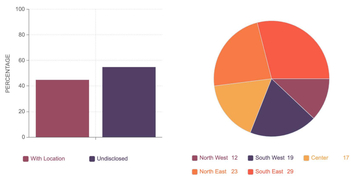
Figure 4 shows the breakdown of tweets with and without the location. The tweets were divided into five zones; north west (Idaho, Montana, Oregon, Washington, and Wyoming), South West (Arizona, Colorado, California, Nevada, New Mexico, and Utah), center ( Iowa, Kansas, Minnesota, Missouri, Nebraska, North Dakota, Oklahoma, and Texas), south east (Arkansas, Alabama, Florida, Georgia, Louisiana, Mississippi, North Carolina, South Carolina, and Tennessee) and all remaining states in north east. Figure 4 shows the percentage of tweets collected from these zones. It can be noted that these zones may not precisely resemble the geographic zones but are organized for ease of analysis. Among the remaining 18432811 tweets, only 6614906 lay in the period around elections and were utilized for positive and negative sentiment analysis in Section 4.1. The remaining 11817905 tweets were employed for retrospective analysis in Section 4.2.
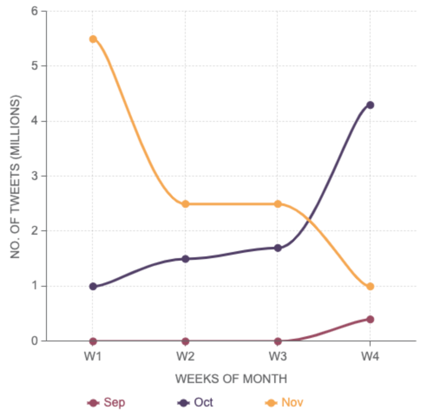
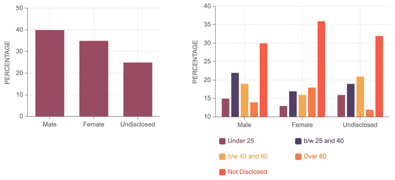
Figure 5 depicts the total number of tweets in different weeks of September, October, and November. It can be noticed that most of the tweets are in the window of mid-October to mid of November. To examine the statistical distribution of data among diverse age and gender groups, Figure 6 provides further insights into data distribution characteristics. It could be observed that the most dominant gender is male with 40%, followed by 35% females. Finally, 25% of the users have either did not disclose their gender or could not be determined directly. It is also interesting to note that most male users are in the age range of 25 and 60. In females, the most dominant users are over 60; however, over-60 users are not very prominent in males. It can also be noted that the female users who do not disclose their age group are higher than males.
The remainder of the section is divided into multiple subsections; Section 4.1 analyzes Twitter sentiment against actual election results. This subsection also identifies extreme positive and negative sentiment for the given candidates and outlier states where election results do not match Twitter sentiments. Section 4.2 inspects shifts in Twitter sentiment before and after elections; negative and positive transitions are highlighted for each candidate. Section 4.3 collates Twitter sentiments between the elections in 2016 and 2020 and identifies sentiment variations after and before Trump’s tenure. Section 4.4 further explains on outlier states and discusses positive and negative sentiment highlighted in Section 4.1. The last section, Section 4.5, analyzes Twitter sentiments during and before elections regarding issues and agendas and identifies which issues earned more attention during the election period.

4.1. Twitter Sentiments and Election Results

For election results analysis, 18,432,811 tweets with locations were considered; only 6,614,906 lay in the period around elections and were employed for positive and negative sentiment analysis for all fifty states, performed for contesting candidates Joe Biden and Donald Trump. The remaining 11,817,905 tweets were used for retrospective analysis, shown in Section 4.2. Table 1 shows the average value of public sentiment obtained two days before, during the elections, in the result compilation phase, and two days after the results. The results are compared with the actual results of the elections. The populations according to the 2019 census in millions is given in the Pop. column of Table 1 [56]. Since the number of tweets (shown in column Tot. Tweets) in a certain state in the recording period are much less than the population, they indicate a sample space for certain sentiments against a given set of hashtags. However, a similar sample set is used for both candidates; therefore, the percentage represents a sufficient indication of public sentiments. The U.S. election results are taken from the BBC website and are given in Elec. (T) and Elec. (B) for Donald Trump (T) and Joe Biden (B), respectively. In most cases, the public sentiment results coincide with the actual election results; however, there are four states where the Twitter sentiment and the actual results are inconsistent. The outliers Arizona, Wisconsin, Georgia, and Pennsylvania are highlighted in black. Further analysis of the Table 1 is as follows:
  • West Virginia, Oklahoma, North Dakota, Montana, Kentucky, Arkansas, and Alabama have the highest positive sentiments for Donald Trump, indicated in green. On the other hand, California, Maine, and New York have the highest positive sentiment for Joe Biden;
  • In contrast, California, Delaware, Hawaii, Illinois, Maryland, and Massachusetts have the highest negative sentiment for Donald Trump, indicated in red. On the other hand, Arkansas, Idaho, Iowa, Kansas, and Kentucky have the most negative sentiment for Joe Biden;
  • Finally, some states have extreme positivity for one candidate and extreme negativity for the contestant. Arkansas and Kentucky have the highest positive sentiment for Donald Trump and the highest negative sentiment for Joe Biden. California has the highest negative sentiment for Donald Trump and the highest positive sentiment for Joe Biden.
Further analysis into outlier states and states with extremely positive and negative sentiments, are analyzed in Section 4.4.

4.2. Pre- and Post-Election Twitter Sentiments Analysis

Elections exhibit a shift in the public’s opinion due to the influence of news, election campaigns, and live debates. The sentiment drift is a subtle phenomenon, as it may have numerous intricate dimensions. This subsection inspects public opinion changes considering tweets during the first week of October and tweets two days before, during, and two days after the results announcement. The average sentiment of one week exactly one month before the election, i.e., 3 October to 10 October 2020, is employed as a pre-election sentiment value. In contrast, the method for post-election is similar to that described in Section 4.1. The primary goal was to determine the shift in public sentiment before and after or during the elections. Among 18,432,811 available tweets with locations, 6,614,906 were used for post-election analysis, while 4,329,302 were employed for pre-election analysis. Table 2 provides positive and negative sentiments for each state before and after the election. All the states with a drift of more than five are highlighted in different color codes; Table 2 shows green and red color codes for increasing and decreasing sentiments in a certain state. It is interesting to remark that eight states have an opposing drift for Trump that decreased in positive sentiment and increased in negative sentiment, i.e., Alabama, Arizona, Florida, Kansas, Maine, Maryland, Massachusetts, and Michigan. Despite the opposing drift, Trump managed to win five states, including Alabama, Arizona, Kansas, Maine, and Michigan.
In terms of the opposing drift positive sentiment in these states, this was much higher for Trump than for Biden. Four states had favoring drift for Trump, including Arkansas, Connecticut, Mississippi, and Nebraska. Notwithstanding favoring drift, Donald Trump lost Connecticut, since Biden had much higher positive sentiment; in other words, Connecticut still selected Biden despite positive sentiments for Trump. Similarly, seven states had an opposing drift for Joe Biden, including Alabama, Arkansas, Illinois, Iowa, Kansas, New York, and Kentucky. Despite having an opposite drift, Joe Biden secured Illinois and New York due to high positive sentiments. Florida was the only state favoring sentiment drift for Joe Biden, but it is an interesting case study. Despite having positive sentiment during the election, favoring drift for Joe Biden, and opposing drift for Trump, Joe Biden lost Florida.

4.3. Comparison of Sentiment Drift during Election of 2016 and 2020

Donald Trump won the election of 2016 by securing 304 electoral votes against 227 electoral votes by Hillary Clinton. The natural extension of sentimental drift analysis is to compare sentiment from the election of 2016. The research provides a state-by-state sentiment analysis of the election of 2016 [48]. Although this research uses a scale of 100 to define positive and negative sentiment, the work considered for the election of 2016 does not use the same scale. However, since, for both candidates, we use the same scale, this does not make a difference in terms of drift analysis. The increase in drift from both positive and negative sentiment scoring more than fifteen and more are highlighted in green, while the negative drift scoring ten or more is highlighted in red. The results of the state-wise analysis are shown in Table 3.
The states with an increase in positive sentiment for Joe Biden from the 2016 election and 2020 election were Colorado, Connecticut, Delaware, Florida, Georgia, Hawaii, Maine, Minnesota, New Hampshire, New Jersey, New York, and Washington. Joe Biden was able to secure victory in all these states. There was an increase in Arkansas, while there was a decrease in negative sentiment for Joe Biden in Maine. In the 2020 elections, Biden was able to win Maine and lost Arkansas, which corroborates with the sentiment analysis results. On the other hand, Donald Trump gained positive sentiment in Alabama, Idaho, Iowa, Kentucky, Louisiana, Mississippi, Montana, Nebraska, North Dakota, Okhalama, and West Virginia. Donald Trump was able to win all states where there was an increase in positive sentiment. There were eleven states where Donald Trump raised negative sentiment; California, Delaware, Hawaii, Illinois, Maine, Maryland, Massachusetts, Rhode Island, South Carolina, Virginia, and Washington. Donald Trump was able to succeed in South Carolina and Virginia and lost the remaining nine states. The only state where there was a reduction in negative sentiment is Hawaii, and Donald Trump lost it.

4.4. Analysis of Outlier and Extreme Sentiments

Table 1 in Section 4.1 shows four outlier states; Arizona, Wisconsin, Georgia, and Pennsylvania. In all four states, the election results were different to the sentiments expressed on Twitter. This subsection analyzes the sentiment in further detail by considering an increase or decrease in both positive and negative sentiments weekly between the last week of September to the third week of November 2020. 
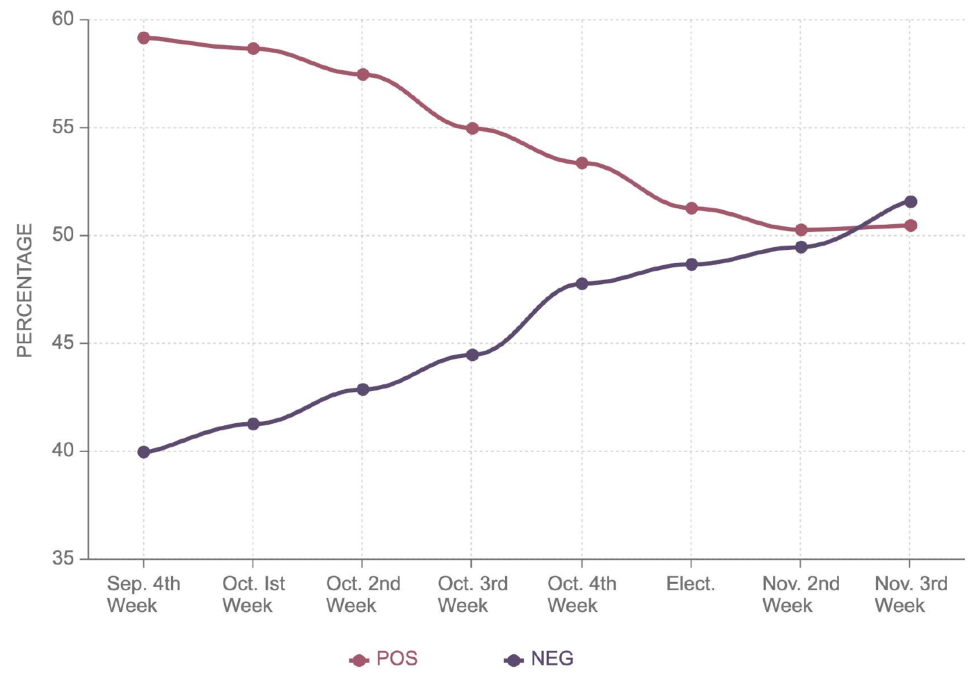
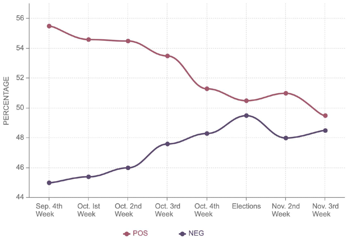
Figure 7 shows a 10% decrease in positive and a 12% increase in negative sentiment. During the elections, it stood as 51.3% positive and 48.7% negative for Donald Trump.
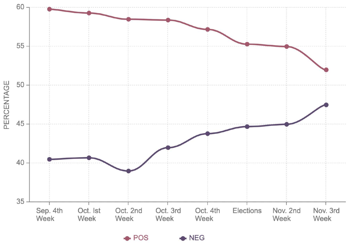
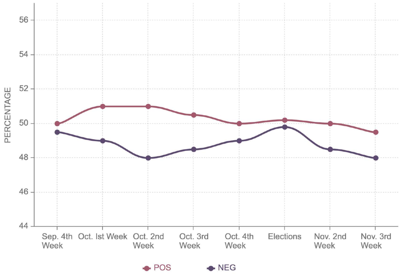
It can be observed that post-election, the negative sentiment further decreased to 52%, surpassing positive sentiment. On the contrary, 
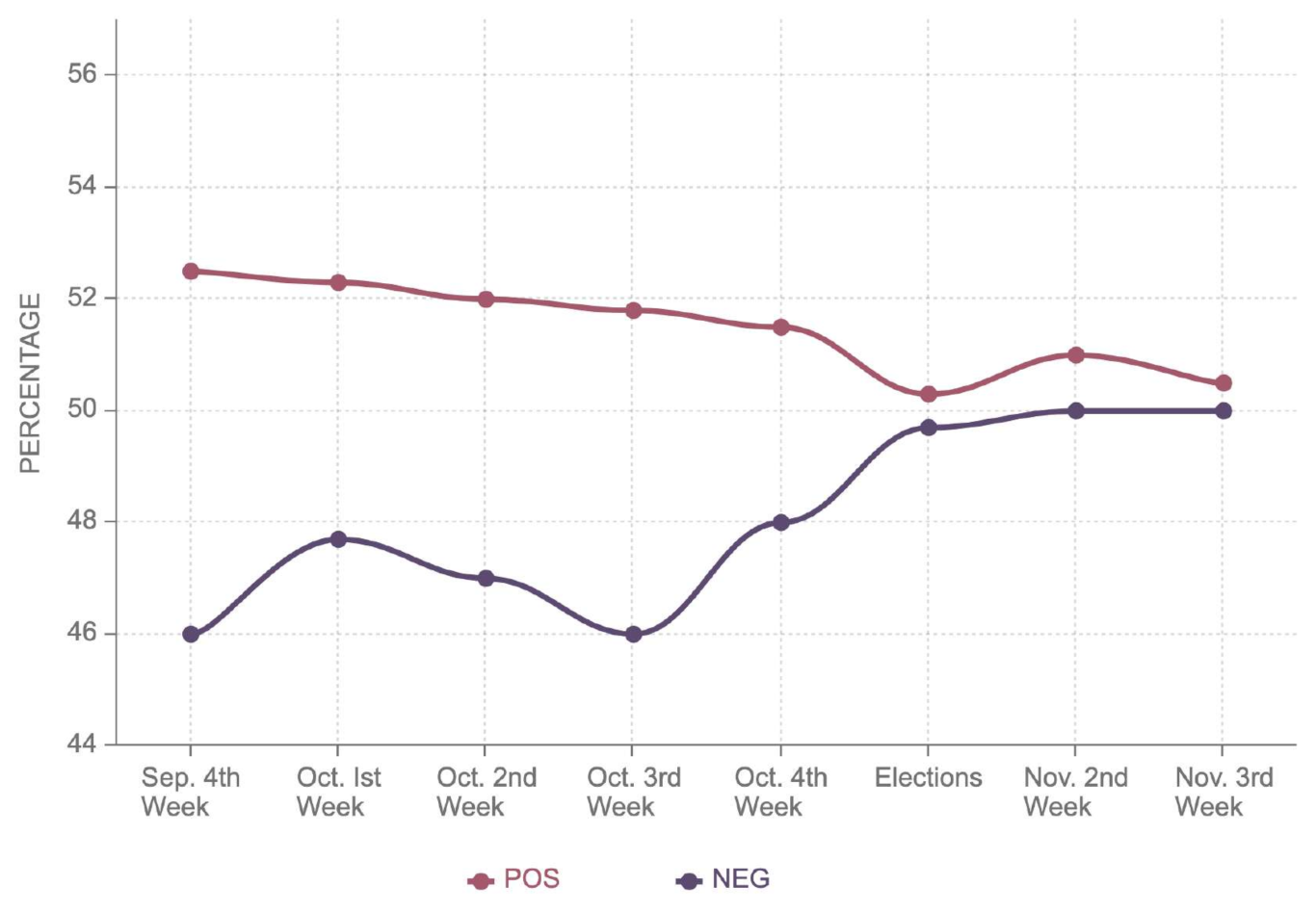
Figure 8 shows that the negative sentiment for Joe Biden decreased from 49.4% to 49%, while the positive sentiment remained almost around 50%. This explains the marginal victory of Joe Biden with 49.4% as compared to 49.1% by Donald Trump. Joe Biden bagged 49.5% of the electoral votes, securing a narrow victory against Trump, who had 49.3% in Georgia. This state is the outlier considering Donald Trump had more positive sentiment, 55.3%, as opposed to 54.5% for Joe Biden. Similarly, he also had less negative sentiment, 44.7%, as compared to Joe Biden’s 45.5%. It can be noted in 
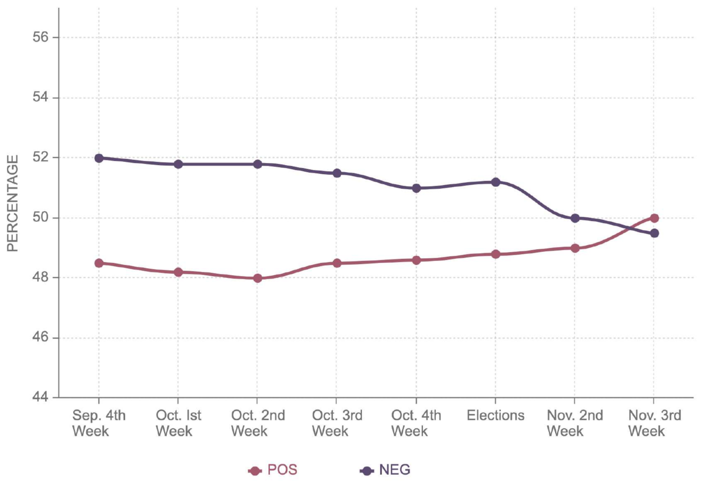
Figure 9 that Biden’s negative sentiment in Georgia decreased steadily, reaching 45.5% two weeks after the election; on the other hand, Trump’s negative sentiment grew to 47%, as shown in Figure 10. Likewise, the positive sentiment of Donald Trump declined by 3% following the election, while positive sentiment for Biden improved by 1%. This illustrates the outcome of the election, even though sentiments were different from the election outcomes.
In terms of sentiments and election result analysis, Pennsylvania shows considerable differences when compared to Georgia and Arizona as shown in Figure 11 and Figure 12. The electoral margin between both candidates was 50%, compared to 48.8% in favor of Joe Biden. However, inspecting the sentimental shift after the election does not provide evidence of an electoral lead. The positive sentiment for both candidates stood at around 50%, while the negative sentiment for both candidates was around 48%. If a long-term sentiment trend is observed, Donald Trump had a much higher positive sentiment a month before the election. Nevertheless, there is no trivial method in our analysis to justify the outlier for Pennsylvania.
Wisconsin was another state where a very narrow competition was anticipated. Joe Biden edged the victory by securing 49.4% of the electoral votes against 48.8% of the electoral votes obtained by Donald Trump. However, the sentiment analysis exhibits 2% more positive sentiment of Donald Trump as compared to Joe Biden. Similarly, Trump had 49.7% while Biden has 51.2% negative sentiment. The comparison of Figure 13 and Figure 14 reveals that both positive and negative sentiments of Trump and Biden were around 50%. However, it can also be noticed that Biden’s negative sentiment decreased from 52% to 50%; on the contrary, the positive sentiment improved from 48% to 50%. The trends for Trump were entirely opposite to that of Joe Biden. This reflects that despite identical sentiments for both candidates, Biden’s repute in the state improved considerably.
Table 4 shows extreme positive and negative sentiments shown in green and red, respectively. Maine had the highest positive sentiment; however, Maine’s margin of victory was lowest among all states with extreme positive sentiment. California seemed the best stronghold for Joe Biden, since the positive sentiment was comparable to Maine. The margin of victory was highest among all states with extreme positive sentiment. Table 5 shows sentiments with extreme negative sentiments for Donald Trump. Despite having the highest negative sentiment, Illinois had the lowest margin of elections in all states with extremely negative sentiment. Table 6 shows extreme positive sentiments: Arkansas had the highest positive sentiment; however, the highest margin of victory was noticed in West Virginia. In most cases, the margin of victory and the sentiment coincided with each other.

4.5. Sentiment Analysis on Policy Matters

The sentiment analysis on policy matters was carried out in states where Trump and Biden won. The sentiment analysis on policy matters was based on keywords used by supporters; we used a predefined dictionary of keywords for each agenda or issue. This revealed which issues were discussed during elections while voting for a particular candidate. In Table 7, it can be seen that the top five issues for states won by Trump were the economy, coronavirus, Supreme Court appointments, foreign policy, and the health care system. On the other hand, the top five issues for states won by Biden were the economy, Supreme Court appointments, immigration policy, the health care system, and coronavirus, as shown in Table 8. Interestingly, the economy, coronavirus, Supreme Court appointments, and health care system are common for states won by both candidates. However, immigration policy is among the most discussed issues for Biden’s states, but it is not among the top five in Trump’s states. Nevertheless, the economy, Supreme Court appointments, health care system and coronavirus are the most discussed issues among both. Among these, Supreme Court appointments and coronavirus were newly emerging issues during these elections, while the economy, the health care system, immigration policy, and foreign policy are recurrent issues.

4.6. Accuracy and Performance Evaluation

We chose thirty thousand tweets to create a training and testing dataset. LIWC was employed to label this dataset, followed by manual inspection. Two thousand tweets were discarded to create a balanced dataset of equally positive and negative class labels, yielding a labeled dataset of twenty-eight thousand tweets. This dataset was partitioned into a 60% training and 40% testing dataset. After training the Naive Bayes classifier, the system was tested over the 40% testing dataset. The confusion matrix for the tested test set of tweets and the results are shown in Table 9. Based on the confusion matrix, the results show the accuracy of 94.58%, with the precision of 93.19% and F1 score of 94.81%, also shown in Table 10. It should be noticed that in Table 10, true positive (TP) stands for the actual class being positive and predicted class being positive, and false negative (FN) stands for the actual class being positive while the predicted class is negative. Moreover, false positive (FP) dnotes that the actual class is negative while the predicted class is negative. Finally, for true negative (TN), the actual class is negative while the predicted class is negative.

5. Future Work

In the future, we plan to find which age groups, gender, and other characteristics correlate with the voting patterns for each candidate. We can employ relationship graphs to find specific patterns among voters from each state voting for certain parties by using graph pattern detection platforms such as [57]. We did not evaluate the seriousness of users before using their tweets for sentiment analysis. Some users might be tweeting just for fun, and their tweets might result in wrong scores in sentiment analysis. The text analysis can also reveal the seriousness of the user before it is used for sentiment analysis; as part of future work, we would apply a seriousness detection algorithm before applying sentiment analysis to improve the accuracy of the work even further.
Some Twitter users might be paid users or party workers who might post trends to boost their party by posting positive tweets or tweeting negatively about their opponents. In this work, we tried to reduce the effect by considering a limited number of tweets per user per day. In future work, pattern detection techniques such as those employed in fake review detection [58] can be used to eliminate such users. The majority of such methods utilize the analysis of writing styles or user behavioral patterns. This would reduce the effect of campaigners or party workers from the sentiment analysis.

6. Conclusions

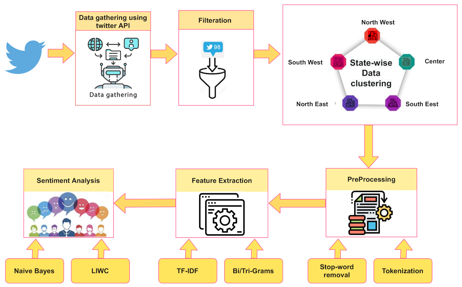
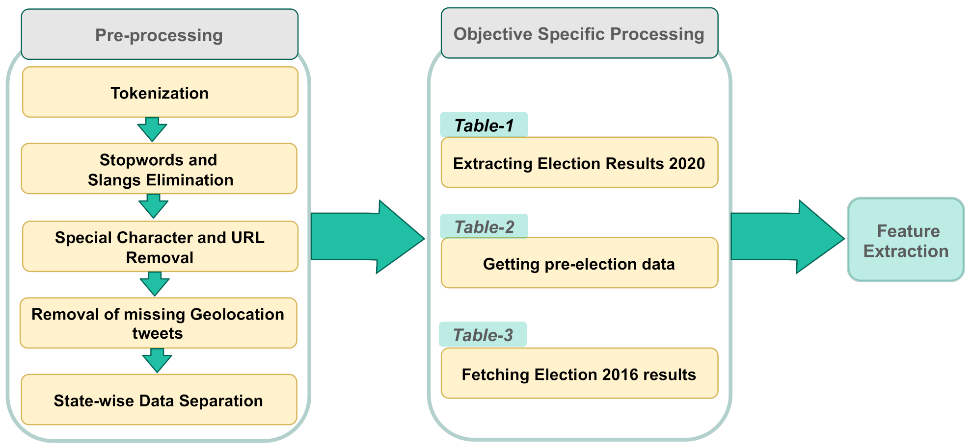
We collected a dataset from Twitter for sentiment analysis of the 2020 U.S. presidential elections. The data were collected before, during, and after the election to measure the public sentiment over social media, and it was compared with the actual election results. The research employed TF-IDF to extract features from the given tweet and used a Naive Bayes classifier to obtain positive or negative sentiment for the given candidate.
In most cases, the public opinion expressed over Twitter coincided with the election results, except four outliers: Arizona, Wisconsin, Georgia, and Pennsylvania. To obtain further insight into outliers, we analyzed sentiment before and after the election. We noticed a sharp decrease in Arizona regarding the positive sentiment of Donald Trump, while Biden’s sentiment remained consistent. Similarly, there was a pattern of increase in the positive sentiment of Biden in Georgia, while Trump’s positive sentiment dropped during the same period. To summarize, for all states where sentiment results did not corroborate with election results, long-term trends before and after the election reveal that there was an increase in the positive sentiment of the winning candidate. At the same time, there was a decrease in positive sentiment for the losing candidate. We conclude that the sentiment analysis results show a similar trend in the presidential elections despite allegations of rigging or election fraud. We also identified that the economy, coronavirus, immigration policy, Supreme Court appointments, and health care systems are important issues on which voters decided to vote for certain parties.

Author Contributions

Conceptualization, U.S., Z.M.; methodology, F.K.; software, H.N.C.; formal analysis, Y.J.; resources, Y.J., Z.I.K.; data curation, Z.I.K.; writing—original draft preparation, H.N.C., F.K.; writing—review and editing, H.N.C., F.K., S.H.J. All authors have read and agreed to the published version of the manuscript.

Funding

The APC was funded by Prince Sultan University.

Acknowledgments

The authors would like to acknowledge the support of Prince Sultan University for paying the Article Processing Charges (APC) of this publication.

Conflicts of Interest

The authors declare no conflict of interest.

References

  1. News, B. US Election 2020 Polls: Who Is Ahead-Trump or Biden? Available online: https://www.bbc.com/news/election-us-2020-53657174 (accessed on 3 November 2020).
  2. IPos. Ipsos Poll Conducted for Thomson Reuters. Available online: https://www.ipsos.com/sites/default/files/ct/news/documents/2020-11/2020_reuters_tracking_-_core_political_general_election_tracker_11_02_2020.pdf (accessed on 2 November 2020).
  3. Yahoo. Yahoo! News Presidential Election-26 October 2020. Available online: https://docs.cdn.yougov.com/fsf95uprtd/20201026_yahoo_coronavirus_tabs.pdf (accessed on 26 October 2020).
  4. WSJNBV. Hart Research Associates/Public Opinion Strategies. Available online: https://s.wsj.net/public/resources/documents/WSJNBCPoll-Mid-October-2020.pdf (accessed on 15 October 2020).
  5. Fox News. 2020 Presidential Election|Fox News. Available online: https://static.foxnews.com/foxnews.com/content/uploads/2020/10/Fox_October-3-6-2020_Complete_National_Topline_October-7-Release-1.pdf (accessed on 10 October 2020).
  6. News, C. CNN, US Pre-Election Analysis. Available online: https://edition.cnn.com/2020/10/30/politics/what-matters-october-29/index.html (accessed on 30 October 2020).
  7. Post, W. ABC News/Washington Post Poll: 2020 Election Update. Available online: https://www.langerresearch.com//wp-content//uploads//1218a12020ElectionUpdate.pdf (accessed on 15 October 2020).
  8. Marieclaire. 2020 Voter Turnout Was the Highest the U.S. Has Seen in Over a Century. Available online: https://www.marieclaire.com/politics/a34589422/voter-turnout-2020/ (accessed on 5 November 2020).
  9. Wang, H.; Can, D.; Kazemzadeh, A.; Bar, F.; Narayanan, S. A system for real-time twitter sentiment analysis of 2012 us presidential election cycle. In Proceedings of the ACL 2012 System Demonstrations, Jeju, Kprea, 8–14 July 2012; pp. 115–120. [Google Scholar]
  10. Nausheen, F.; Begum, S.H. Sentiment analysis to predict election results using Python. In Proceedings of the 2018 2nd International Conference on Inventive Systems and Control (ICISC), Coimbatore, India, 19–20 January 2018; IEEE: Piscataway, NJ, USA, 2018; pp. 1259–1262. [Google Scholar]
  11. Caetano, J.A.; Lima, H.S.; Santos, M.F.; Marques-Neto, H.T. Using sentiment analysis to define twitter political users’ classes and their homophily during the 2016 American presidential election. J. Internet Serv. Appl. 2018, 9, 18. [Google Scholar] [CrossRef] [Green Version]
  12. Jose, R.; Chooralil, V.S. Prediction of election result by enhanced sentiment analysis on Twitter data using Word Sense Disambiguation. In Proceedings of the 2015 International Conference on Control Communication Computing India (ICCC), Trivandrum, India, 19–21 November 2015; pp. 638–641. [Google Scholar] [CrossRef]
  13. Singhal, K.; Agrawal, B.; Mittal, N. Modeling Indian general elections: Sentiment analysis of political Twitter data. In Information Systems Design and Intelligent Applications; Springer: Berlin/Heidelberg, Germany, 2015; pp. 469–477. [Google Scholar]
  14. Salari, S.; Sedighpour, N.; Vaezinia, V.; Momtazi, S. Estimation of 2017 Iran’s Presidential Election Using Sentiment Analysis on Social Media. In Proceedings of the 2018 4th Iranian Conference on Signal Processing and Intelligent Systems (ICSPIS), Tehran, Iran, 25–27 December 2018; IEEE: Piscataway, NJ, USA, 2018; pp. 77–82. [Google Scholar]
  15. Choy, M.; Cheong, M.L.; Laik, M.N.; Shung, K.P. A sentiment analysis of Singapore Presidential Election 2011 using Twitter data with census correction. arXiv 2011, arXiv:1108.5520. [Google Scholar]
  16. Cerón-Guzmán, J.A.; León-Guzmán, E. A sentiment analysis system of Spanish tweets and its application in Colombia 2014 presidential election. In Proceedings of the IEEE International Conferences on Big Data and Cloud Computing (BDCloud), Social Computing and Networking (Socialcom), Sustainable Computing and Communications (Sustaincom)(BDCloud-Socialcom-Sustaincom), Atlanta, GA, USA, 8–10 October 2016; IEEE: Piscataway, NJ, USA, 2016; pp. 250–257. [Google Scholar]
  17. Salloum, S.A.; Al-Emran, M.; Monem, A.A.; Shaalan, K. A survey of text mining in social media: Facebook and twitter perspectives. Adv. Sci. Technol. Eng. Syst. J. 2017, 2, 127–133. [Google Scholar] [CrossRef] [Green Version]
  18. Imtiaz, S.; Horchidan, S.F.; Abbas, Z.; Arsalan, M.; Chaudhry, H.N.; Vlassov, V. Privacy Preserving Time-Series Forecasting of User Health Data Streams. In Proceedings of the 2020 IEEE International Conference on Big Data (Big Data), Atlanta, GA, USA, 10–13 December 2020; IEEE: Piscataway, NJ, USA, 2020; pp. 3428–3437. [Google Scholar]
  19. Wang, H.; Bah, M.J.; Hammad, M. Progress in outlier detection techniques: A survey. IEEE Access 2019, 7, 107964–108000. [Google Scholar] [CrossRef]
  20. Stefanovič, P.; Kurasova, O. Outlier detection in self-organizing maps and their quality estimation. Neural Netw. World 2018, 28, 105–117. [Google Scholar] [CrossRef]
  21. Pang, B.; Lee, L.; Vaithyanathan, S. Thumbs up? Sentiment classification using machine learning techniques. arXiv 2002, arXiv:cs/0205070. [Google Scholar]
  22. Turney, P.D. Thumbs up or thumbs down? Semantic orientation applied to unsupervised classification of reviews. arXiv 2002, arXiv:cs/0212032. [Google Scholar]
  23. Cumani, S.; Laface, P.; Kulsoom, F. Speaker recognition by means of acoustic and phonetically informed GMMs. In Proceedings of the Sixteenth Annual Conference of the International Speech Communication Association, Dresden, Germany, 6–10 September 2015; pp. 200–204. [Google Scholar]
  24. Usman Sarwar, M.; Rehman Javed, A.; Kulsoom, F.; Khan, S.; Tariq, U.; Kashif Bashir, A. Parciv: Recognizing physical activities having complex interclass variations using semantic data of smartphone. Softw. Pract. Exp. 2021, 51, 532–549. [Google Scholar] [CrossRef]
  25. Narejo, S.; Pasero, E.; Kulsoom, F. EEG based eye state classification using deep belief network and stacked autoencoder. Int. J. Electr. Comput. Eng. (IJECE) 2016, 6, 3131–3141. [Google Scholar] [CrossRef]
  26. Kalsum, T.; Mehmood, Z.; Kulsoom, F.; Chaudhry, H.N.; Khan, A.R.; Rashid, M.; Saba, T. Localization and classification of human facial emotions using local intensity order pattern and shape-based texture features. J. Intell. Fuzzy Syst. 2021, 40, 9311–9331. [Google Scholar] [CrossRef]
  27. Janjua, S.H.; Siddiqui, G.F.; Sindhu, M.A.; Rashid, U. Multi-level aspect based sentiment classification of Twitter data: Using hybrid approach in deep learning. PeerJ Comput. Sci. 2021, 7, e433. [Google Scholar] [CrossRef] [PubMed]
  28. Pradhan, R.; Khandelwal, V.; Chaturvedi, A.; Sharma, D.K. Recommendation System using Lexicon Based Sentimental Analysis with collaborative filtering. In Proceedings of the 2020 International Conference on Power Electronics IoT Applications in Renewable Energy and its Control (PARC), Mathura, India, 28–29 February 2020; pp. 129–132. [Google Scholar] [CrossRef]
  29. Guo, X.; Li, J. A novel twitter sentiment analysis model with baseline correlation for financial market prediction with improved efficiency. In Proceedings of the 2019 Sixth International Conference on Social Networks Analysis, Management and Security (SNAMS), Granada, Spain, 22–25 October 2019; IEEE: Piscataway, NJ, USA, 2019; pp. 472–477. [Google Scholar]
  30. Cardie, C.; Farina, C.; Bruce, T. Using natural language processing to improve erulemaking: Project highlight. In Proceedings of the 2006 International Conference on Digital Government Research, San Diego, CA, USA, 21–24 May 2006; pp. 177–178. [Google Scholar]
  31. Mukwazvure, A.; Supreethi, K. A hybrid approach to sentiment analysis of news comments. In Proceedings of the 2015 4th International Conference on Reliability, Infocom Technologies and Optimization (ICRITO)(Trends and Future Directions), Noida, India, 2–4 September 2015; IEEE: Piscataway, NJ, USA, 2015; pp. 1–6. [Google Scholar]
  32. Štrimaitis, R.; Stefanovič, P.; Ramanauskaitė, S.; Slotkienė, A. Financial Context News Sentiment Analysis for the Lithuanian Language. Appl. Sci. 2021, 11, 4443. [Google Scholar] [CrossRef]
  33. Singh, V.K.; Piryani, R.; Uddin, A.; Waila, P. Sentiment analysis of movie reviews: A new feature-based heuristic for aspect-level sentiment classification. In Proceedings of the 2013 International Mutli-Conference on Automation, Computing, Communication, Control and Compressed Sensing (iMac4s), Kottayam, India, 22–23 March 2013; IEEE: Piscataway, NJ, USA, 2013; pp. 712–717. [Google Scholar]
  34. Jin, X.; Li, Y.; Mah, T.; Tong, J. Sensitive Webpage Classification for Content Advertising. In Proceedings of the 1st International Workshop on Data Mining and Audience Intelligence for Advertising, ADKDD ’07, San Jose, CA, USA, 12 August 2007; Association for Computing Machinery: New York, NY, USA, 2007; pp. 28–33. [Google Scholar] [CrossRef]
  35. Liu, R.; Yao, X.; Guo, C.; Wei, X. Can We Forecast Presidential Election Using Twitter Data? An Integrative Modelling Approach. Ann. GIS 2021, 27, 43–56. [Google Scholar] [CrossRef]
  36. Baker Al Barghuthi, N.; E. Said, H. Sentiment Analysis on Predicting Presidential Election: Twitter Used Case. In Intelligent Computing Systems; Brito-Loeza, C., Espinosa-Romero, A., Martin-Gonzalez, A., Safi, A., Eds.; Springer International Publishing: Cham, Switzerland, 2020; pp. 105–117. [Google Scholar]
  37. Sharma, P.; Moh, T.S. Prediction of Indian election using sentiment analysis on Hindi Twitter. In Proceedings of the 2016 IEEE International Conference on Big Data (Big Data), Washington, DC, USA, 5–8 December 2016; IEEE: Piscataway, NJ, USA, 2016; pp. 1966–1971. [Google Scholar]
  38. Unankard, S.; Li, X.; Sharaf, M.; Zhong, J.; Li, X. Predicting Elections from Social Networks Based on Sub-event Detection and Sentiment Analysis. In Web Information Systems Engineering–WISE 2014; Benatallah, B., Bestavros, A., Manolopoulos, Y., Vakali, A., Zhang, Y., Eds.; Springer International Publishing: Cham, Switzerland, 2014; pp. 1–16. [Google Scholar]
  39. Kagan, V.; Stevens, A.; Subrahmanian, V. Using twitter sentiment to forecast the 2013 pakistani election and the 2014 indian election. IEEE Intell. Syst. 2015, 30, 2–5. [Google Scholar] [CrossRef]
  40. Oyebode, O.; Orji, R. Social media and sentiment analysis: The nigeria presidential election 2019. In Proceedings of the 2019 IEEE 10th Annual Information Technology, Electronics and Mobile Communication Conference (IEMCON), Vancouver, BC, Canada, 17–19 October 2019; IEEE: Piscataway, NJ, USA, 2019; pp. 140–146. [Google Scholar]
  41. Singh, A.K.; Gupta, D.K.; Singh, R.M. Sentiment Analysis of Twitter User Data on Punjab Legislative Assembly Election, 2017. Int. J. Mod. Educ. Comput. Sci. 2017, 9, 60–68. [Google Scholar]
  42. Kristiyanti, D.A.; Umam, A.H.; Normah. Prediction of Indonesia presidential election results for the 2019–2024 period using twitter sentiment analysis. In Proceedings of the 2019 5th International Conference on New Media Studies (CONMEDIA), Bali, Indonesia, 9–11 October 2019; IEEE: Piscataway, NJ, USA, 2019; pp. 36–42. [Google Scholar]
  43. Razzaq, M.A.; Qamar, A.M.; Bilal, H.S.M. Prediction and analysis of Pakistan election 2013 based on sentiment analysis. In Proceedings of the 2014 IEEE/ACM International Conference on Advances in Social Networks Analysis and Mining (ASONAM 2014), Beijing, China, 17–20 August 2014; IEEE: Piscataway, NJ, USA, 2014; pp. 700–703. [Google Scholar]
  44. Budiharto, W.; Meiliana, M. Prediction and analysis of Indonesia Presidential election from Twitter using sentiment analysis. J. Big Data 2018, 5, 1–10. [Google Scholar] [CrossRef] [Green Version]
  45. Liu, B. Sentiment analysis and opinion mining. Synth. Lect. Hum. Lang. Technol. 2012, 5, 1–167. [Google Scholar] [CrossRef] [Green Version]
  46. Yaqub, U.; Chun, S.A.; Atluri, V.; Vaidya, J. Sentiment based analysis of tweets during the us presidential elections. In Proceedings of the 18th Annual International Conference on Digital Government Research, Staten Island, NY, USA, 7–9 June 2017; pp. 1–10. [Google Scholar]
  47. Joyce, B.; Deng, J. Sentiment analysis of tweets for the 2016 US presidential election. In Proceedings of the 2017 IEEE MIT Undergraduate Research Technology Conference (URTC), Cambridge, MA, USA, 3–5 November 2017; IEEE: Piscataway, NJ, USA, 2017; pp. 1–4. [Google Scholar]
  48. Agrawal, A.; Hamling, T. Sentiment analysis of tweets to gain insights into the 2016 US election. Columbia Undergrad. Sci. J. 2017, 11, 3. [Google Scholar]
  49. Paul, D.; Li, F.; Teja, M.K.; Yu, X.; Frost, R. Compass: Spatio temporal sentiment analysis of US election what twitter says! In Proceedings of the 23rd ACM SIGKDD International Conference on Knowledge Discovery and Data Mining, Halifax, NS, Canada, 13–17 August 2017; pp. 1585–1594. [Google Scholar]
  50. Chen, E.; Deb, A.; Ferrara, E. # Election2020: The first public Twitter dataset on the 2020 US Presidential election. J. Comput. Soc. Sci. 2021, 34, 1–18. [Google Scholar]
  51. Endsuy, R.D. Sentiment Analysis between VADER and EDA for the US Presidential Election 2020 on Twitter Datasets. J. Appl. Data Sci. 2021, 2, 08–18. [Google Scholar]
  52. Ebrahimi, M.; Yazdavar, A.H.; Sheth, A. Challenges of sentiment analysis for dynamic events. IEEE Intell. Syst. 2017, 32, 70–75. [Google Scholar] [CrossRef] [Green Version]
  53. Robertson, S. Understanding inverse document frequency: On theoretical arguments for IDF. J. Doc. 2004, 60, 503–520. [Google Scholar] [CrossRef] [Green Version]
  54. Jurafsky, D. Speech & Language Processing; Pearson Education India: Noida, India, 2000. [Google Scholar]
  55. Zhang, H. The optimality of naive Bayes. AA 2004, 1, 3. [Google Scholar]
  56. Bureau, U.C. United States of America Population, Census 2019; United States Census Bureau: Suitland, ML, USA, 2019. [Google Scholar]
  57. Chaudhry, H.N. FlowGraph: Distributed temporal pattern detection over dynamically evolving graphs. In Proceedings of the 13th ACM International Conference on Distributed and Event-Based Systems, Darmstadt, Germany, 24–28 June 2019; pp. 272–275. [Google Scholar]
  58. Heydari, A.; ali Tavakoli, M.; Salim, N.; Heydari, Z. Detection of review spam: A survey. Expert Syst. Appl. 2015, 42, 3634–3642. [Google Scholar] [CrossRef]
Figure 1. Flow diagram of sentiment analysis on Twitter data.
Electronics 10 02082 g001
Figure 2. Percentage of sizes of collected tweets.
Electronics 10 02082 g002
Figure 3. Detailed diagram showing pre-processing and additional result-specific stages.
Electronics 10 02082 g003
Figure 4. Zone-wise user location of tweets.
Electronics 10 02082 g004
Figure 5. Collection time period of tweets.
Electronics 10 02082 g005
Figure 6. Age group and gender distribution of users.
Electronics 10 02082 g006
Figure 7. Graphs of positive and negative sentiments of Donald Trump in Arizona.
Electronics 10 02082 g007
Figure 8. Graphs of positive and negative sentiments of Joe Biden in Arizona.
Electronics 10 02082 g008
Figure 9. Graphs of positive and negative sentiments of Joe Biden in Georgia.
Electronics 10 02082 g009
Figure 10. Graphs of positive and negative sentiments of Donald Trump in Georgia.
Electronics 10 02082 g010
Figure 11. Graphs of positive and negative sentiments of Donald Trump in Pennsylvania.
Electronics 10 02082 g011
Figure 12. Graphs of positive and negative sentiments of Joe Biden in Pennsylvania.
Electronics 10 02082 g012
Figure 13. Graphs of positive and negative sentiments of Donald Trump in Wisconsin.
Electronics 10 02082 g013
Figure 14. Graphs of positive and negative sentiments of Biden in Wisconsin.
Electronics 10 02082 g014
Table 1. U.S. Election results 2020 and comparison with Twitter sentiment.
NameAbbr.Pop.Tot.Tweets%pos(T)%Neg(T)Elec(T)%pos(B)%neg(B)Elec(B)
AlabamaAL4.9105,65462.4%37.6%62.0%46.3%53.7%36.6%
AlaskaAK0.73340558.2%41.8%52.8%45.9%54.1%42.8%
ArizonaAZ7.28172,34951.3%48.7%49.1%49.5%50.5%49.4%
ArkansasAR3.0275,80962.5%37.5%62.4%37.9%62.1%34.8%
CaliforniaCA39.51491,30339.1%60.9%34%64.2%35.8%64%
ColoradoCO5.76119,80844%56%42%54.2%45.9%55%
ConnecticutCT3.5791,40543.8%56.2%39%57.4%42.6%59%
DelawareDE0.97690539.5%60.5%40%56.4%43.6%59%
FloridaFL21.48326,57847.3%52.7%51.2%58.4%41.6%47.9%
GeorgiaGA10.62265,67855.3%44.7%49.3%54.5%45.5%49.5%
HawaiiHI1.4227,80937.5%62.5%34.3%57.2%42.8%63.7%
IdahoID1.7954,60057.6%42.4%63.8%39.2%60.8%33.1%
IllinoisIL12.67289,00435.9%64.1%40.5%54.5%45.5%57.5%
IndianaIN6.73139,80154.3%45.7%57.0%43.9%56.1%41.0%
IowaIA3.1689,02058.5%41.5%53.1%46.7%52.3%44.9%
KansasKS2.9155,60955.5%44.5%56.1%47.3%52.7%41.5%
KentuckyKY4.47112,00061.2%38.8%62.1%41.5%58.5%36.2%
LouisianaLA4.65107,89158.4%41.6%58.5%41.8%58.2%39.9%
MaineME1.3419,88442.4%57.6%44.0%64.3%35.7%53.0%
MarylandMD6.05128,80837.4%62.6%32.3%55.4%44.6%65.7%
Massach.MA6.89154,60639%61%32.1%57%43%65.6%
MichiganMI9.99261,76747.5%52.5%47.8%54.5%45.5%50.6%
MinnesotaMN5.64123,79045.8%54.2%52.4%57.3%42.7%45.3%
Missi.MS2.9891,90958.4%41.6%57.5%43.5%56.5%41.0%
MissouriMO6.14146,50756.4%43.6%56.7%45.8%54.2%41.4%
MontanaMT1.0712,40061.3%38.7%56.7%43%57%40.4%
NebraskaNE1.9345,60458.6%42.4%58.5%44.5%55.5%39.3%
NevadaNV3.0881,90951%49%47.7%50.1%49.9%50.1%
New Hamp.NH1.3634,50948%52%45.5%57.4%42.6%52.8%
New JerseyNJ8.88215,60048.5%51.5%41.3%55.5%44.5%57.1%
New MexicoNM2.160,56044.6%55.4%43.5%53.4%46.6%54.3%
New YorkNY19.45364,32343.8%56.2%37.7%61%39%60.9%
North Car.NC10.49223,94556%44%49.9%51.5%48.5%48.6%
North Dak.ND0.76989061.4%38.6%65.1%45%55%31.8%
OhioOH11.69314,56352.5%47.5%53.3%48.7%51.3%45.2%
OklahomaOK3.96109,89060.9%39.1%65.4%43.7%56.3%32.3%
OregonOR4.22100,20446.1%53.9%40.4%54%46%56.5%
PennsylvaniaPA12.8256,57850.5%49.5%48.8%50.2%49.8%50.0%
Rhode IslandRI1.06789040.6%59.4%38.6%43.7%56.3%59.4%
South Car.SC5.15114,50243.6%56.4%55.1%52.3%47.7%43.4%
South Dak.SD0.8812,50652.3%47.7%61.8%50.2%49.8%35.6%
TennesseeTN6.83161,50757.4%42.6%60.7%46%54%37.5%
TexasTX29352,44151.6%48.4%52.0%49.5%50.5%46.5%
UtahUT3.2197,89057.6%42.4%58.1%47.5%52.5%37.6%
VermontVT0.62500144%56%30.7%55.3%44.7%66.1%
VirginiaVA8.54194,35641.8%58.2%44.0%52.3%47.7%54.1%
WashingtonWA7.61203,42142%58%39.0%57.6%42.4%58.4%
West Virg.WV1.7935,60761.2%38.8%68.6%40.5%59.5%29.7%
WisconsinWI5.82134,50650.3%49.7%48.8%48.8%51.2%49.4%
WyomingWY0.58340559.3%40.7%69.9%43%57%26.6%
Table 2. Pre and post-election sentiment drift of users on Twitter.
Pre-Election (Trump)Post-Election (Trump)Pre-Election (Biden)Post-Election (Biden)
NameAbbr.%Pos%Neg%Pos%Neg%Pos%Neg%Pos%Neg
AlabamaAL69%31%62.4%37.6%52.2%47.8%6.3%53.7%
AlaskaAK57.9%42.1%58.2%41.8%46.2%53.8%45.9%54.1%
ArizonaAZ58.7%41.3%51.3%48.7%50.1%49.9%49.5%51.5%
ArkansasAR57.9%42.1%62.5%37.5%48.1%51.9%37.9%62.1%
CaliforniaCA35.8%64.2%39.1%60.9%65.4%34.6%64.2%35.8%
ColoradoCO45.1%54.9%44%56%58.5%41.5%54.2%45.9%
Connecti.CT38.2%61.8%43.8%56.2%59%41%57.4%42.6%
DelawareDE36.5%64.5%39.5%60.5%59.5%40.5%56.4%43.6%
FloridaFL57%43%47.3%52.7%51%49%58.4%41.6%
GeorgiaGA59.3%40.7%55.3%44.7%52.3%47.7%54.5%45.5%
HawaiiHI39.4%60.6%37.5%62.5%59.3%40.7%57.2%42.8%
IdahoID59.5%40.5%57.6%42.4%39.9%60.1%39.2%60.8%
IllinoisIL39%61%35.9%64.1%61.5%38.5%54.5%45.5%
IndianaIN58.5%41.5%54.3%45.7%44.3%55.7%43.9%56.1%
IowaIA57.4%42.6%58.5%41.5%53.3%46.7%46.7%52.3%
KansasKS60.2%39.8%55.5%44.5%52.7%47.3%47.3%52.7%
KentuckyKY65.5%34.5%61.2%38.8%48.7%51.3%41.5%58.5%
LouisianaLA57%43%58.4%41.6%45%55%41.8%58.2%
MaineME47.9%52.1%42.4%57.6%61.4%38.6%64.3%35.7%
MarylandMD46.6%53.4%37.4%62.6%54%46%55.4%44.6%
Massach.MA44%56%39%61%56.7%43.3%57%43%
MichiganMI52.4%47.6%47.5%52.5%53.4%46.6%45.5%50.6%
MinnesotaMN47.5%52.5%45.8%54.2%55.2%44.8%57.3%42.7%
Missi.MS52%48%58.4%41.6%47%53%43.5%56.5%
MissouriMO54.3%45.7%56.4%43.6%47.7%52.3%45.8%54.2%
MontanaMT58.5%41.5%61.3%38.7%43.7%56.3%43%57%
NebraskaNE53%47%58.6%42.4%47.9%52.1%44.5%55.5%
NevadaNV52.5%47.5%51%49%48%52%50.1%49.9%
New Hamp.NH49.5%50.5%48%52%55%45%57.4%42.6%
New JerseyNJ50.3%49.7%48.5%51.5%55.2%44.8%55.5%44.5%
New Mex.NM45.7%54.3%44.6%55.4%52.9%47.1%53.4%46.6%
New YorkNY47%53%43.8%56.2%54%46%61%39%
North Car.NC55.4%44.6%56%44%50.3%49.7%51.5%48.5%
North Dak.ND57.1%42.9%61.4%38.6%47.6%52.4%45%55%
OhioOH50.1%49.9%52.5%47.5%49.2%50.8%48.7%51.3%
OklahomaOK58%42%60.9%39.1%47.6%52.4%43.7%56.3%
OregonOR46.3%53.7%46.1%53.9%52.2%47.8%54%46%
Pennsyl.PA54.6%45.4%50.5%49.5%51%49%50.2%49.8%
Rhode Isl.RI43.7%56.3%40.6%59.4%46.5%53.5%43.7%56.3%
South Car.SC47.6%52.4%43.6%56.4%51.3%48.7%52.3%47.7%
South Dak.SD53.5%46.5%52.3%47.7%50.1%49.9%50.2%49.8%
TennesseeTN56.3%43.7%57.4%42.6%49%51%46%54%
TexasTX51.3%48.7%51.6%48.4%49.9%50.1%49.5%50.5%
UtahUT55.3%44.7%57.6%42.4%48.7%51.3%47.5%52.5%
VermontVT48%52%44%56%55.1%44.9%55.3%44.7%
VirginiaVA45.5%54.5%41.8%58.2%51.9%48.1%52.3%47.7%
WashingtonWA40%60%42%58%55.1%44.9%57.6%42.4%
West Virg.WV60.9%39.1%61.2%38.8%40.6%59.4%40.5%59.5%
WisconsinWI52.3%47.7%50.3%49.7%48.2%51.8%48.8%51.2%
WyomingWY57.3%42.7%59.3%40.7%44%56%43%57%
Table 3. Sentiment drift of users in elections of 2016 and 2020.
Elec. 2016 (Rep.)Elec. 2020 (Rep.)Elect. 2016 (Dem.)Elect. 2020 (Dem.)
NameAbbr.%Pos%Neg%Pos%Neg%Pos%Neg%Pos%Neg
AlabamaAL43.2%42.2%62.4%37.6%37.2%48.9%46.3%53.7%
AlaskaAK45.7%39.4%58.2%41.8%45.7%39.7%45.9%54.1%
ArizonaAZ44.7%42.9%51.3%48.7%37.3%49.4%49.5%51.5%
ArkansasAR44.5%41.6%62.5%37.5%39.1%46.6%37.9%62.1%
CaliforniaCA42.6%44.0%39.1%60.9%40.6%45.7%64.2%35.8%
ColoradoCO42.4%44.1%44%56%39.8%47.0%54.2%45.9%
ConnecticutCT42.1%44.0%43.8%56.2%41.0%45.0%57.4%42.6%
DelawareDE40.0%45.4%39.5%60.5%41.7%43.5%56.4%43.6%
FloridaFL44.6%40.9%47.3%52.7%37.6%48.3%58.4%41.6%
GeorgiaGA44.6%41.5%55.3%44.7%39.3%47.4%54.5%45.5%
HawaiiHI48.4%38.8%37.5%62.5%37.4%49.5%57.2%42.8%
IdahoID43.2%43.9%57.6%42.4%34.5%53.0%39.2%60.8%
IllinoisIL42.7%44.1%35.9%64.1%41.5%45.0%54.5%45.5%
IndianaIN42.5%43.4%54.3%45.7%40.2%45.6%43.9%56.1%
IowaIA43.5%43.3%58.5%41.5%41.1%45.3%46.7%52.3%
KansasKS43.4%43.9%55.5%44.5%39.9%45.7%47.3%52.7%
KentuckyKY45.5%41.4%61.2%38.8%37.0%50.1%41.5%58.5%
LouisianaLA37.6%40.6%58.4%41.6%35.5%44.7%41.8%58.2%
MaineME41.4%42.9%42.4%57.6%38.6%45.5%64.3%35.7%
MarylandMD44.4%41.8%37.4%62.6%42.8%44.7%55.4%44.6%
MassachusettsMA42.0%44.4%39%61%43.4%43.1%57%43%
MichiganMI43.8%41.7%47.5%52.5%40.4%44.3%45.5%50.6%
MinnesotaMN44.5%42.0%45.8%54.2%42.7%43.4%57.3%42.7%
MississippiMS44.0%39.5%58.4%41.6%37.5%47.8%43.5%56.5%
MissouriMO44.7%42.4%56.4%43.6%47.8%48.4%45.8%54.2%
MontanaMT42.9%43.1%61.3%38.7%34.6%50.5%43%57%
NebraskaNE43.5%42.3%58.6%42.4%39.5%45.5%44.5%55.5%
NevadaNV44.6%42.6%51%49%38.1%48.8%50.1%49.9%
New HampshireNH44.7%41.8%48%52%40.3%45.8%57.4%42.6%
New JerseyNJ42.5%43.8%48.5%51.5%39.3%47.3%55.5%44.5%
New MexicoNM43.7%43.4%44.6%55.4%39.0%48.7%53.4%46.6%
New YorkNY42.7%44.1%43.8%56.2%42.6%43.2%61%39%
North CarolinaNC44.7%42.6%56%44%41.0%45.8%51.5%48.5%
North DakotaND47.8%40.7%61.4%38.6%38.1%49.2%45%55%
OhioOH43.7%42.6%52.5%47.5%41.1%45.2%48.7%51.3%
OklahomaOK44.5%41.5%60.9%39.1%39.9%45.4%43.7%56.3%
OregonOR43.1%44.9%46.1%53.9%40.4%47.2%54%46%
PennsylvaniaPA44.8%41.8%50.5%49.5%40.9%45.5%50.2%49.8%
Rhode IslandRI42.9%45.0%40.6%59.4%40.5%46.7%43.7%56.3%
South CarolinaSC44.3%40.3%43.6%56.4%38.7%47.2%52.3%47.7%
South DakotaSD45.2%40.1%52.3%47.7%41.4%44.3%50.2%49.8%
TennesseeTN46.0%40.1%57.4%42.6%38.8%48.4%46%54%
TexasTX44.4%42.0%51.6%48.4%37.6%48.2%49.5%50.5%
UtahUT44.2%40.7%57.6%42.4%42.0%43.3%47.5%52.5%
VermontVT42.5%47.3%44%56%44.0%44.2%55.3%44.7%
VirginiaVA44.3%42.8%41.8%58.2%38.1%49.2%52.3%47.7%
WashingtonWA42.4%44.7%42%58%41.5%45.1%57.6%42.4%
West VirginiaWV45.4%41.6%61.2%38.8%38.8%47.6%40.5%59.5%
WisconsinWI43.4%42.8%50.3%49.7%41.8%44.2%48.8%51.2%
WyomingWY46.5%41.9%59.3%40.7%41.1%48.8%43%57%
Table 4. Biden: extreme positive and negative sentiment states with margin of victory.
MaineCaliforniaNew YorkArkansasIdaho
Sentiments64.3%64.2%61%62.1% 60.8%
Margin of Victory9%30%23.2%−27.6%−30.7%
Table 5. Trump: extreme negative sentiment states with margin of victory.
IllinoisMarylandHawaiiCaliforniaDelaware
Sentiments 64.1% 62.6% 62.5% 60.9% 60.5%
Margin of Victory−17%−33.4%−29.4%−30%19%
Table 6. Trump: extreme positive sentiment states.
ArkansasAlabamaNorth DakotaMontanaKentuckyWest VirginiaOklahoma
Sentiments62.5%62.4%61.4%61.3%61.2%61.2% 60.9%
Margin of Victory27.6%26%33.3%16%25.8%38.9%33.1%
Table 7. Sentiment analysis based on agenda issues, sorted on states won by Trump.
Agenda IssueTrump’s StatesBiden’s States
Economy21%29%
Coronavirus18%10%
Supreme Court Appointments11%14%
Foreign Policy10%9%
Health Care System10%11%
Violence and Crime9%4%
Ethical Inequality8%5%
Immigration Policy8%15%
Climate Change4%2%
LGBT and other issues1%1%
Table 8. Sentiment analysis based on agenda issues, sorted on states won by Biden.
Agenda IssueTrump’s StatesBiden’s States
Economy21%29%
Supreme Court Appointments11%14%
Immigration Policy8%15%
Health Care System10%11%
Coronavirus18%10%
Foreign Policy10%9%
Ethical Inequality8%5%
Violence and Crime9%4%
Climate Change4%2%
LGBT and other issues1%1%
Table 9. Confusion matrix of Naive Bayes classifier.
Actual PositiveActual Negative
Predicted Positive0.4940.035
Predicted Negative0.0180.45
Table 10. Accuracy, precision, recall and F1 score based on confusion matrix.
MetricValueFormulation
Sensitivity0.9648 T P R = T P / ( T P + F N )
Specificity0.9259 S P C = T N / ( F P + T N )
Precision0.9319 P P V = T P / ( T P + F P )
Negative Predictive Value0.9615 N P V = T N / ( T N + F N )
False Positive Rate0.0741 F P R = F P / ( F P + T N )
False Discovery Rate0.0681 F D R = F P / ( F P + T P )
False Negative Rate0.0352 F N R = F N / ( F N + T P )
Accuracy0.9458 A C C = ( T P + T N ) / ( P + N ) )
F1 Score0.9481 F 1 = 2 T P / ( 2 T P + F P + F N )
Publisher’s Note: MDPI stays neutral with regard to jurisdictional claims in published maps and institutional affiliations.

