Face Recognition via Deep Learning Using Data Augmentation Based on Orthogonal Experiments

Abstract

Class attendance is an important means in the management of university students. Using face recognition is one of the most effective techniques for taking daily class attendance. Recently, many face recognition algorithms via deep learning have achieved promising results with large-scale labeled samples. However, due to the difficulties of collecting samples, face recognition using convolutional neural networks (CNNs) for daily attendance taking remains a challenging problem. Data augmentation can enlarge the samples and has been applied to the small sample learning. In this paper, we address this problem using data augmentation through geometric transformation, image brightness changes, and the application of different filter operations. In addition, we determine the best data augmentation method based on orthogonal experiments. Finally, the performance of our attendance method is demonstrated in a real class. Compared with PCA and LBPH methods with data augmentation and VGG-16 network, the accuracy of our proposed method can achieve 86.3%. Additionally, after a period of collecting more data, the accuracy improves to 98.1%.

1. Introduction

Taking class attendance in university classes is one of the commonly used methods to improve the performance of students studies in many universities. Louis et al. [1] highlights a strong relevance between student’s attendance and academic performance; low attendance is usually correlated with poor performance. To guarantee the correctness of a student’s attendance record, a proper approach is required for verifying and managing the attendance records. The traditional attendance-taking approach is to pass an attendance sheet around the classroom during class, and to request students sign their names. Another popular approach is roll call, by which the instructor records the attendance by calling the name of each student. One advantage of these manual attendance-taking methods is that they require no special environment or equipment. However, there are two obvious disadvantages in these manual methods. First, these methods not only waste a lot of valuable class time, but also have the risk of including imposters. Second, the form of class attendance records is hard to manage and easy to be lost if not careful. As a result of the progress of technologies, there are many new attendance-taking systems available, e.g., RFID [2], bluetooth [3], GPS [4], fingerprint [5,6], face [7,8,9], etc. The above problems related to the traditional attendance-taking methods can be handled by these new attendance-taking methods, in particular, those that use face recognition.

Face recognition is one of the most attractive biometric technologies. With the rapid development of technology, the accuracy of face recognition has greatly improved. Many methods for face recognition have been proposed and applied to many areas, such as face identification, security, surveillance, access control, identity verification [10,11,12], and so on. There are three advantages of using face recognition in a class attendance-taking method. First, it reduces the burden for the instructor and the students. Also, it can prevent imposters of assuming the attendance of registered students of the class. Last but not least, the operation required from an instructor involves taking a picture of the class using a smartphone without any additional hardware or setup in the classroom.

Recently, with the emergence of deep learning, face recognition achieves impressive results. A convolutional neural network (CNN), one of the most popular deep neural networks in computer vision applications, shows an important advantage of automatic visual feature extraction [13]. There are two kinds of methods to train CNN for face recognition, one is based on the classification layer [14], and another is based on metric learning. The main idea of metric learning for face recognition is maximizing interclass variance and minimizing intraclass variance. For example, FaceNet [15] uses triplet loss to learn the Euclidean space embedding in which all faces of one identity can be projected onto a single point. Sphereface [16] proposes angular margin penalty to enforce extra intraclass compactness and interclass discrepancy simultaneously. The authors of [17] propose an Additive Angular Margin Loss function that can effectively enhance the discriminative power of feature embeddings learned via CNNs for face recognition. CNNs trained on 2D face images can effectively work for 3D face recognition by fine-tuning the CNN with 3D facial scans [18]. In addition, the three-dimensional context is invariant to lightening/make-up/camouflage conditions. The authors of [19] take some linear quantities as measures and rely on differential geometry to extract relevant discriminant features from the query faces. Meanwhile, Nicole et al. [20] propose an automatic approach to compute a minimum optimized marker layout to be exploited in facial motion capture. Despite considerable success in 2D and 3D recognition, face recognition using CNNs in class attendance-taking encounters some challenging problems, such as difficulty in getting sufficient training samples, because CNNs require a lot of data for training. Generally, a large volume of training samples are helpful to achieve a high recognition accuracy. Overfitting usually occurs when the quantity of training samples is small compared with the number of network parameters. As a result, an insufficient number of samples decreases the accuracy of face recognition. Because a CNN has a powerful learning ability, it requires for each object different views of its face. However, collecting such a dataset for only one class is not only time-consuming, but also impractical. Additionally, training samples of faces of various poses, occlusion, and illumination are often required. Meanwhile, it is difficult, if not impossible, for the instructor to spend too much time taking photos during class. Due to the restriction of time and scene, it is difficult to acquire enough face images in class.

To address the issue of insufficient samples, an effective method is the data augmentation technique [21,22]. The basic idea of data augmentation is to generate virtual samples to increase the size of training dataset and reduce overfitting. In this paper, geometric transformation, changes in image brightness, and operation using different filter operations are utilized to enlarge the training samples. In addition, we analyze the effect of the above processing methods on the accuracy of face recognition using the method of orthogonal experiments. Then, the original training samples are extended by the best data augmentation method based on the result of the orthogonal experiments. Finally, we compare our proposed class attendance-taking method with two typical face recognition algorithms, namely, Principal Component Analysis (PCA) and Local Binary Patterns Histograms (LBPH). The result shows that our class attendance-taking method with data augmentation achieves an accuracy of 86.3%, and with more data collected during a term, the accuracy can be improved to 98.1%.

The rest of this paper is organized as follows. In Section 2, the related works are presented. Section 3 describes our method. The experiments and results are presented in Section 4. Section 5 contains discussions. Finally, our conclusions are presented in Section 6.

2. Related Works

Manual class attendance-taking methods are time-consuming and inaccurate, especially in large classes. As a result, automated attendance system can help improve the quality and efficiency of class attendance. Modern attendance-taking systems generally consist of hardware and software. There are many successful cases of using automated attendance-taking systems. Mittal et al. [23] propose an attendance-taking system based on a fingerprint recognition device. To attend a class, students are recognized based on their fingerprints. As well, the fingerprint recognition device can be connected to a computer through an USB interface so that the instructor can manage the attendance records. This system provides a simple method to generate the attendance record automatically and reduces the risk of fraudulent attendance by imposters. However, students need to line up to get their fingerprints recognized, which is consuming for a large class. In addition, the fingerprint recognition device is usually very sensitive, and a sweaty finger or a finger with cut may fail to be recognized as a legitimate registered student. Nguyen et al. [24] develop an attendance-taking system using Radio Frequency Identification (RFID). Each student is issued a unique RFID card. To register for attendance, students only need to place their RFID cards by an RFID tag reader. The attendance information is kept on a website, allowing instructors to view or modify the records easily. Recently, some instructors use smartphones to capture class attendance. Pinter et al.  [25] design an application for smartphones based on the bluetooth technique. When taking attendance, students turn on the bluetooth of their smartphones and choose a class from a class list for registering. Finally, instructors can login to their apps and see the IDs and names of students who have attended the class. Allen et al. [26] use smartphones as a QR code reader to speed up taking attendance. At the beginning of a class, the instructor displays an encrypted QR code on a screen for students to scan it using a special app installed on their smartphones. Along with the student’s geographical position at the time of scan, the application will then communicate the information collected with the server to confirm attendance of the student automatically. These automated attendance-taking methods are faster than traditional manual methods. In addition, the operation is simple and the attendance record is easy to access or manipulate. With an automated attendance-taking system, instructors can save lecture time and, thus, enhance student learning experience. However, these methods also have some drawbacks. First, most of the above methods require special equipments such as the fingerprint recognition device or an RFID tag reader. If all the classrooms were equipped with these devices, the total cost would be high for schools with many classrooms. Second, any damages to the equipment, such as an RFID card or the reader, may create incorrect attendance records. Third, some methods still cannot avoid imposters. For example, a student can bring other students’ phones or RFID cards to help them fake their attendance.

Face recognition is one of the commonly used biometric identification methods in the field of computer vision. An attendance-taking system based on face recognition generally includes image acquisition, creating a dataset, face detection, and face recognition. Unlike a fingerprint, a face can be recognized easily by a human. Thanks to its convenience in acquisition and reliable and friendly interaction, human face recognition systems have become an important tool in automatic attendance-taking systems. Rathod et al. [27] develop an automated attendance-taking system based on face detection and recognition algorithms. After installing the camera in a classroom, it captures the frames containing the faces of all students sitting in the class. Then the student’s face region is extracted and preprocessed for further processing. Later, this system can automatically detect and recognize each student. After recognizing the faces of students, the names are updated into an Excel spreadsheet. In addition, an antispoofing technique, like the eye blink detector, is used to handle the spoofing of face recognition. In particular, the count of detected eyes and the count of iris regions detection are compared. Based on this, the count of eye blink can be calculated to handle spoofing. Wei et al. [28] solve the problem of in-class social network construction and pedagogical analysis with a multimedia technique. In data acquisition, an instructor takes some photos of students in a class and these photos are combined into a single image using an image stitching algorithm. Then, the course website allows the instructor to upload the stitched photo. Then, face detection, student localization, and face recognition algorithms are used to identify students’ names and positions. Then, students login in the website to check their attendance to complete the attendance record and annotate their faces with their names after each class. At the end of the semester, their sitting positions can be used to construct the social network. With the statistics of social network, students’ academic performance and the pedagogical analysis about co-learning patterns can be constructed automatically.

Recently, a number of research papers have been published on using deep neural networks in the field of facial biometrics with impressive results. Compared with traditional algorithms [29] for face recognition, CNNs are trained using a data-driven network architecture. In addition, CNN models combine feature extraction and classifier into one framework [30]. A CNN model mainly includes convolutional layers, pooling layers, fully-connected layers, as well as an input and an output layer. Based on its shared-weight, local connectivity and subsampling, CNNs are better in extracting features and making significant breakthrough in face recognition. Taigman et al. [14] propose a DeepFace model based on an architecture of CNN. This model is trained with 4.4 million face images of 4000 identities on the LFW (Labeled Faces in the Wild) dataset and reaches an accuracy of 97.25%. Sun et al. [31] develop a model named DeepID that has multiple CNNs rather than a single CNN, by which a powerful feature extractor is developed. The input of DeepID is patches of facial images and features extracted from different facial positions. The DeepID model is trained on 202,599 images and reaches an accuracy of 97.45%. Then, Sun et al. propose an extension of DeepID called as DeepID2 [32], which uses both identification and verification signals to reduce intraclass variations while enlarging the interclass differences. DeepID2 is also trained on 202,599 images and reaches an accuracy of 99.15%. Later, DeepID2+ [33] is proposed to improve the performance of DeepID2. DeepID2+ adds supervisory signals to all convolutional layers and increases the dimension of each layer. Additionally, DeepID2+ is trained on a larger training dataset which contains 450,000 images. Additionally, DeepID2+ achieves an accuracy of 99.47%. Schroff et al. [15] propose the FaceNet model, which learns the mapping from a face image to an Euclidean space, in which the distance of two faces measures their similarity. On the LFW dataset, FaceNet achieves an accuracy of 99.63% with 200 million training samples. Simonyan et al. [34] propose a deep CNNs architecture named VGG-16 and achieve an accuracy of 98.95% with 2.6 million images. This model requires fewer training data than DeepFace and FaceNet and uses a simpler network than DeepID2. However, building such a large dataset is beyond the capabilities of most academia groups especially in the context of taking class attendance. In this paper, we propose a system that can alleviate the above discussed issues.

3. Our Method

3.1. Orthogonal Design of Experiments

The first step of this phase is determining the experimental factors and choose the proper levels. The choice of which experimental factors to use tends to be based on the professional knowledge and experience [35], so we choose the common data augmentation methods such as image zoom, translation, rotation, brightness, and four kinds of filter operations as the factors. As to the experimental level, we only choose three kinds of levels for each factor, as too many levels increases the experimental run time. The levels of each data augmentation method are shown in

Table 1. The parameters of data augmentation methods with different levels.

Methods	Parameters	Level 1	Level 2	Level 3
Image zoom	scale coefficient	1.2	1.5	1.8
Image translation	$(\Delta x,\Delta y)$ in Equation (1)	(12,10)	(18,15)	(24,20)
Image rotation	rotate angle $\theta$	10	25	40
Image brightness	scale coefficient	1.2	1.5	1.8
Mean filter	window size	$3\times 3$	$4\times 4$	$5\times 5$
Median filter	window size	$3\times 3$	$5\times 5$	$7\times 7$
Gaussian filter	window size	$3\times 3$	$5\times 5$	$7\times 7$
Bilateral filter	window size	$3\times 3$	$5\times 5$	$7\times 7$

. In this paper, to reduce the the times of experiments, we divided the factors into two parts: one is the geometric transformation and image brightness, and the other is the factors including image filters; a $L_9\left(3^4\right)$ orthogonal table is used to arrange the four factors with three levels for each part.

3.2. Deep CNN for Class Attendance Taking

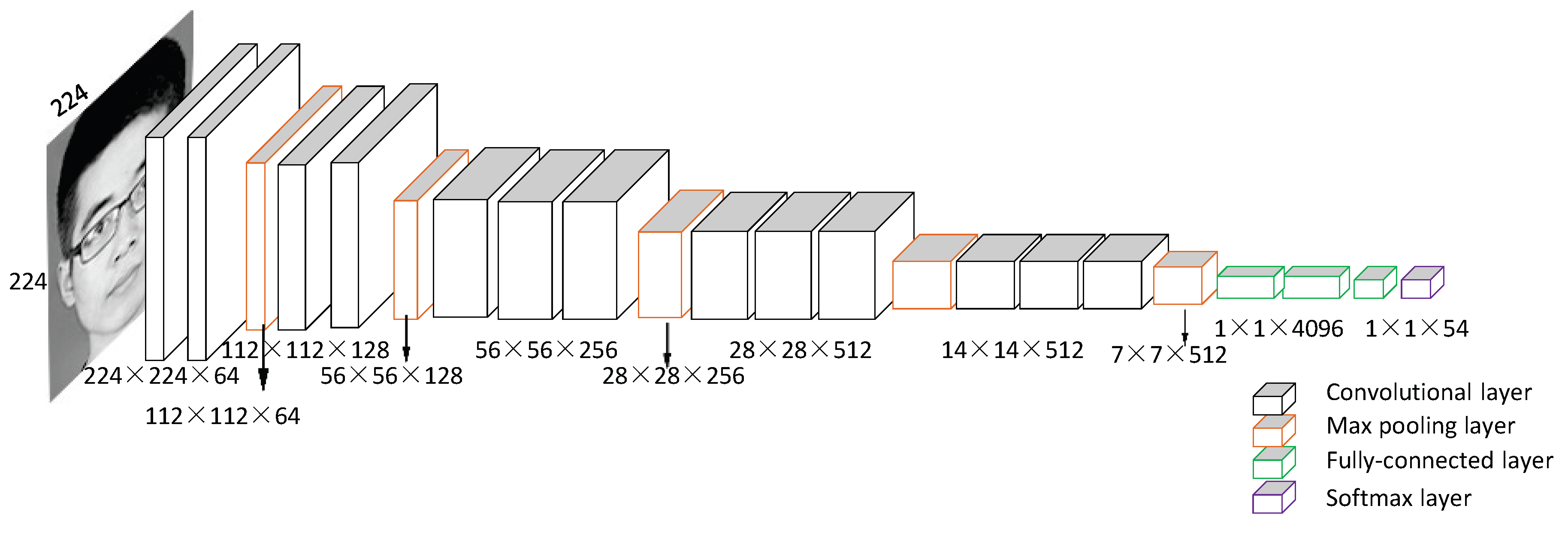
In this experiment, we fine-tune the VGG-16 network pretrained with a VGG-Face dataset to accomplish face recognition. Fine-tuning is an approach that initializes the CNN model parameters for the target task from the parameters pretrained on another related task [36]. As shown in Figure 1, the input of the net is a fixed RGB image of 224 × 224; this deep CNN architecture mainly consists of thirteen convolutional layers, five pooling layers, and three fully-connected layers; the last fully-connected layer has 54 channels since there are 54 identities in the class. The VGG-16 architecture increases the depth of network by adding many convolutional layers with the kernel of size 3 × 3 and these small convolution kernels make it work successfully. The spatial resolution is preserved after convolution with the spatial padding of 1 and the convolution stride of 1. Downsampling is carried out by five max pooling layers, which follow some of convolutional layers (not all the convolutional layers are followed by pooling layers). The max pooling layers are performed over a 2 × 2 pixel window with a stride of 2. ReLU activation functions are used in the convolutional and fully-connected layers, whereas a softmax function is used in the final layer.

The training dataset is used to train the model, and the forward propagation is used to compute the output of different layers in the neural network. Denote the output feature map of the convolutional layer as C,

$$C=\varphi \left(H\right(x,y\left)\right),$$

(1)

where $\varphi (.)$ denotes the ReLU function $\varphi \left(H\right(x,y\left)\right)=max(0,H(x,y\left)\right)$ and

$$H(x,y)=\sum _{m,n\in s}W(m,n)I_i^{\prime }(x+m,y+n)+b,$$

(2)

where W denotes the weight matrix of kernel and b the bias. $\varphi (.)$ is used as the activation function; compared with other activation functions like tanh and sigmoid, the output of the ReLU function can reduce the computation and accelerate the convergence of the network. In addition, with the increase of absolute value of $H(x,y)$, the gradient of sigmoid or tanh function approaches 0. Thus, the sigmoid and tanh activation functions are prone to the vanishing gradient problem, whereas ReLU does not have such a problem when $H(x,y)>0$.

The convolutional layer is followed by the max pooling layer with a 2 × 2 kernel. A pooling layer is used to reduce the spatial size and the number of parameters in the network. It can prevent overfitting as well. The output map of the pooling layer denoted as P can be calculated by

$$P=g\left(C\right),$$

(3)

where $g(.)$ denotes the function to calculate the max value. As the window moves across C, $g(.)$ selects the largest value in the window and discards the rest. Dropout layers are used to alleviate overfitting. In a dropout layer, the output of a neuron is set to 0 with a probability of 0.5 at each update during the training phase. These neurons are “dropped out” and do not contribute to the forward propagation and back-propagation, which helps prevent overfitting.

Later, the output of the fully-connected layer at neuron q denoted as $F_q$ is computed as

$$F_q=\varphi (\sum _{m,n\in s}W(m,n)P(x,y)+b).$$

(4)

Then, the softmax-loss function denoted as L is used as the network’s loss function, and our model is trained with the MBGD (Mini-Batch Gradient Descent) method,

$$L=-\frac{1}{M}\sum _{i=1}^M\sum _q^J{T}_{i}log\left(p_q\right),$$

(5)

where M denotes the number of images in a batch of one iteration (batch size set to 64) and $p_q$ the output of the network at neuron q, i.e., the probability of the model’s prediction which can be calculated by the softmax function,

$$p_q=\frac{exp\left(F_q\right)}{{\sum }_{Z=1}^{J}exp\left(F_Z\right)}.$$

(6)

The back-propagation algorithm is used to update the weight w, and the update rule is

$$\Delta v_t=\mu \Delta v_{t-1}-\alpha \frac{\partial L}{\partial w},$$

(7)

$$w_t^{\prime }=w_t+\Delta v_t,$$

(8)

where $\mu$ denotes the momentum coefficient which can accelerate convergence (we used $\mu$ = 0.9), $\Delta v_{t-1}$ denotes the previous updated value of weight, $w_t$ denotes the current weight at iteration t, and $\alpha$ denotes the learning rate, the basic learning rate ${\alpha }_0$ is 0.001. The update rule of $\alpha$ is

$${\alpha }_j={\alpha }_{j-1}\ast {\gamma }^{\frac{t}{u}},$$

(9)

where $\gamma$ denotes the gamma parameter($\gamma =0.1$) and u the stepsize (u is 10,000).

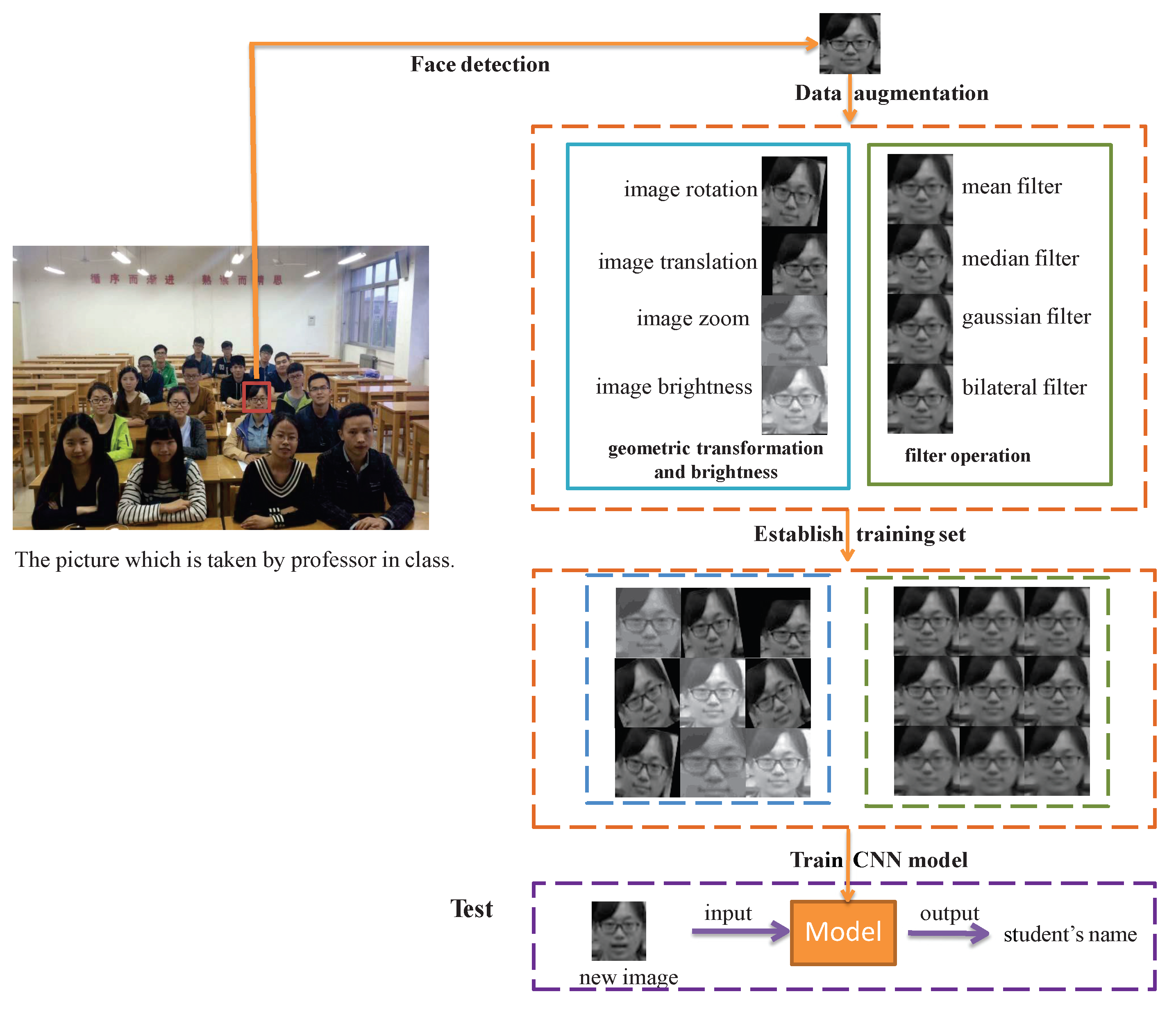
The workflow of our method is shown in Figure 2 and Algorithm 1. First, the original training samples from class pictures are acquired using a face detection algorithm. Second, data augmentation is used to increase the number of training samples using geometric transformation, image brightness manipulation or filter operations. Then, the CNN model is trained with the augmented training samples. During testing, an unknown student’s image is input to the trained model, then the output is the name of the student.

3.3. Analysis of Results

To demonstrate the performance of face recognition, it is evaluated by 5-fold cross-validation. The range analysis method is used to analyze the effect of different augmentation methods. Usually, compared with other analysis methods, the range analysis is more intuitive. The range value denoted as R indicates that the corresponding factor has a greater importance.

3.4. Implementation Details

The data augmentation algorithms are based on the Python2.7 with OpenCV in Ubuntu 16.04 and are derived from the publicly available python Caffe toolbox. For hyperparameters in the phase of VGG-16 network fine-tuning, the basic learning rate ${\alpha }_0$ is 0.001 with $\gamma =0.1$, and the stepsize is 10,000. The VGG-16 model is pretrained with VGG-Face dataset. We use 3538 students’ face images for fine-tuning and 372 face images for validating. The batch size is 64, and the max iteration is 50,000. The model is fine-tuned on a single NVIDIA Titan Xp 12GB GPU with a Caffe deep learning framework [37] and takes about 8 h for each experiment.

Additionally, to guarantee the smooth completion of the class attendance taking process, the attendance website can be used as a supplement for face recognition. At the end of each class, the instructor submits the photo taken in class to the website. If a face is not automatically detected by the website, the student can login to the website and manually select their face’s region to complete the record. Additionally, if the face recognition fails to produce a correct attendance record, students can manually choose their faces to correct the record. Besides, for each student who is absent in the attendance record, the web-based system automatically sends an email to remind them to check if it was a failure of the face recognition system and, if so, identify the appropriate face in the class photo to correct the attendance record.

Algorithm 1 Class attendance taking using a convolutional neural network

1: Capture all students’ face images; 2: Augment training samples and establish the training dataset; 3: for each iteration t to max iterations do 4:  if t % stepsize == 0 then 5:   Update learning rate $\alpha$ using Equation (18); 6:  end if 7:  for each training image $I_k^{\prime }$ do 8:   Compute the output of each layer by the forward propagation algorithm via Equation (10), Equation (11), Equation (12) and Equation (13); 9:  end for 10:  Update weight $\omega$ by the back propagation algorithm via Equations (16) and (17); 11: end for 12: for each test image do 13:  Compute the output of each layer using forward propagation algorithm by Equation (10), Equation (11), Equation (12) and Equation (13); 14:  Compute the output of network p using Equation (15); 15:  Print the student’s name; 16: end for

4. Experiment and Results

4.1. Data Collection

To collect original face images, we design a website that can automatically detect a student’s face based on an AdaBoost algorithm with a skin color model [38]. The instructor takes a photo of the students at the beginning of the first several classes in a term, and in each class, a single image including all the students’ faces is captured. After each class, the instructor submits the image to the attendance taking website. Similar to supervised learning methods, the training samples are annotated before using them for training. However, this procedure is time-consuming. To simplify this problem, students are asked to login in the website and choose their faces and annotate them with their IDs. Students follow these steps to annotate their face images annotation in the first few classes. In this paper, suppose each class has J students, the set of collected original face images is denoted as $I=\left\{I_k\right|k\in [1,N]\}$, where $I_k$ denotes a face image and N denotes the total number of original images.

4.2. Data Augmentation

As the number of original face images is insufficient for training a deep CNN model, a common method is to enlarge the training set using the method of data augmentation by generating multiple virtual images from each original image using geometric transformation, image brightness manipulation, and filter operations.

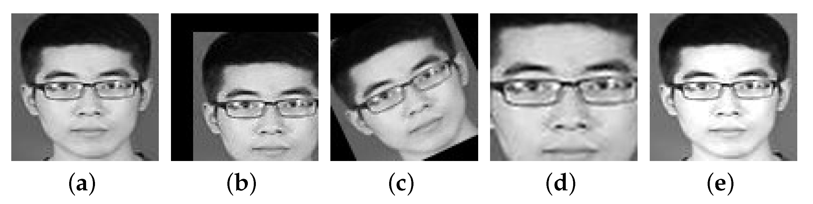
The geometric transformation includes image translation, image rotation, and image zoom (see Figure 3b–d). Image translation refers to moving the image to a new position. For each image $I_k$ where $k=1,\cdots ,N$, $I_k(x,y)$ denotes the pixel’s value at $(x,y)$, the translated image denotes as $I_k^T$ is given by

$$I_k^T(x,y)=I_k(x+\Delta x,y+\Delta y),$$

(10)

where $\Delta x$ and $\Delta y$ denote the shifting in horizontal and vertical direction. The rotated image $I_k^R$ is generated by

$$I_k^R(x,y)=I_k(xcos\theta -ysin\theta ,xsin\theta +ycos\theta ),$$

(11)

where $\theta$ denotes the rotated angle. The zoomed image $I_k^Z$ is generated using bilinear interpolation with Equation (3).

$$I_k^Z(x,y)=I_k(c_{x}x,c_{y}y),$$

(12)

where $c_x$ and $c_y$ denote the zoom factor in the horizontal and vertical directions, respectively. An image brightness enhancement algorithm is used to generate a new image by changing the brightness. The corresponding image $I_k^B$ can be obtained by

$$I_k^B(x,y)=I_k(x,y)+\tau ,$$

(13)

where $\tau$ denotes the bias parameter of brightness.

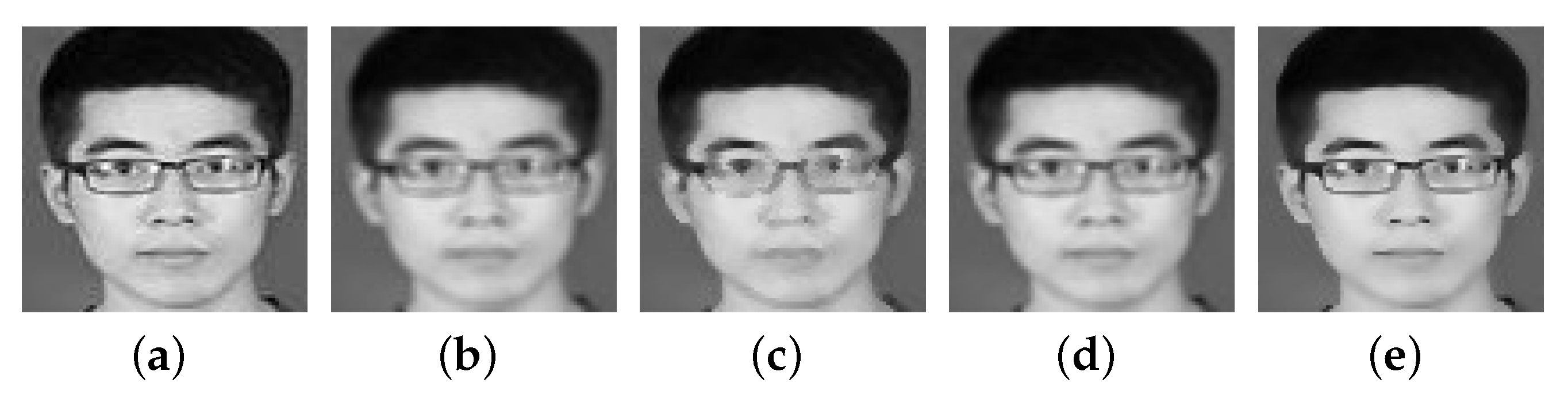
The filter operations include mean filter, median filter, Gaussian filter, and bilateral filter (see Figure 4). With different filter operations for each image $I_k$, the corresponding virtual images $I_k^{Mean}$, $I_k^{Med}$, $I_k^{Gau}$, and $I_k^{Bil}$ are generated. The mean filter is used to smooth an image that replaces the central value by the average of all the pixels in the nearby window. The equation is

$$I_k^{Mean}(x,y)=\frac{1}{S}\sum _{(m,n)\in s}{I}_k(x+m,y+n),$$

(14)

where S is the total number of pixels of the kernel in the neighborhood s; m and n denote $m_{th}$ row and $n_{th}$ column in the kernel, respectively. Similarly, a median filter is usually used to reduce noise and replace the central pixel with the median value of the nearby pixels. The image $I_{med}^d$ is generated by

$$I_k^{Med}(x,y)=f\left(I_k(x+m,y+n)\right)(m,n)\in s,$$

(15)

where $f(.)$ denotes a function to compute median value. A Gaussian filter is a two-dimensional convolution operator, which follows a Gaussian distribution. The central value is replaced by the weighted average of neighbouring pixels, and the central pixel has the heaviest weight while nearby pixels have smaller weights. Its equation is

$$I_k^{Gau}(x,y)=\sum _{(m,n)\in s}G(m,n)I_k(x+m,y+n),$$

(16)

where $G(m,n)$ denotes the weight of the Gaussian kernel. A bilateral filter is similar to a Gaussian filter, which can reduce noise and preserve edge fairly sharp. The update of the center value is replaced by the weighted average of nearby pixels. The image $I_k^{Bil}$ can be obtained via

$$I_k^{Bil}(x,y)=\frac{{\sum }_{(m,n)\in s}{I}_k(x+m,y+n)E(x,y,x+m,y+n)}{{\sum }_{(m,n)\in s}E(x,y,x+m,y+n)},$$

(17)

and $E(.)$ denotes the normalization factor

$$E(x,y,x+m,y+n)=exp(-\frac{m^2+n^2}{2{\sigma }_s^2}-\frac{\left|\right|I_k(x,y)-I_k(x+m,y+n){\left|\right|}^2}{2{\sigma }_r^2}),$$

(18)

where ${\sigma }_s$ and ${\sigma }_r$ denote the spatial and range kernel’s parameters of the Gaussian function, respectively.

After data augmentation of the set I of original face images, the augmented set of images denoted as $I^{\prime }=\{I_k^T,I_k^R,I_k^Z,I_k^B,I_k^{Mean},I_k^{Med},I_k^{Gau},I_k^{Bil}|k\in [1,N]\}$ can be generated. In supervised learning, each input sample has a corresponding category label. Denote the training dataset as $D=\left\{(I_i^{\prime },T_i)\right|i\in [1,U]\}$, where $I_i^{\prime }$ denotes a training image from $I^{\prime }$, $T_i$ is the corresponding label, and U is the total number of training images.

4.3. Cross Validation

In

Table 2. The orthogonal experiment of geometric transformation and image brightness.

	Image Zoom	Image Translation	Image Rotation	Image Brightness	Accuracy
1	1	1	1	1	83.3%
2	1	2	2	2	79.6%
3	1	3	3	3	81.5%
4	2	1	2	3	83.3%
5	2	2	3	1	83.3%
6	2	3	1	2	83.3%
7	3	1	3	2	83.3%
8	3	2	1	3	85.2%
9	3	3	2	1	81.5%
K1	244.4	249.9	251.8	248.1
K2	249.9	248.1	244.4	246.2
K3	250	246.3	248.1	250.0
$\overline{k1}$ = K1/3	81.47	83.30	83.93	82.70
$\overline{k2}$ = K2/3	83.30	82.70	81.47	82.07
$\overline{k3}$ = K3/3	83.33	82.10	82.70	83.33
R	1.86	1.20	2.46	1.26

, we compare the different combinations of levels and factors on data augmentation methods, where $Kl$ denotes the sum of the lth current factor and $\overline{kl}$ denotes the average of $Kl$. Table 2 shows that the largest range value is image rotation, which indicates that image rotation is the primary factor, and the effect of factors is listed in descending order as follows; image rotation > image zoom > image brightness > image translation. According to this table, we also can determine the best combination of geometric transformation and image brightness is to use the 3rd level of image zoom, 1st level of image translation, 1st level of image rotation, and 3rd level of image brightness. The results of orthogonal experiments on filter operation are shown in

Table 3. The orthogonal experiment of filter operation.

	Mean Filter	Median Filter	Gaussian Filter	Bilateral Filter	Accuracy
1	1	1	1	1	81.5%
2	1	2	2	2	77.8%
3	1	3	3	3	79.6%
4	2	1	2	3	79.6%
5	2	2	3	1	85.2%
6	2	3	1	2	77.8%
7	3	1	3	2	79.6%
8	3	2	1	3	81.5%
9	3	3	2	1	79.6%
K1	238.9	240.7	240.8	246.3
K2	242.6	244.5	237	235.2
K3	240.7	237	244.4	240.7
$\overline{k1}$ = K1/3	79.63	80.23	80.27	82.10
$\overline{k2}$ = K2/3	80.87	81.50	79.00	78.40
$\overline{k3}$ = K3/3	80.23	79.00	81.47	80.23
R	1.24	2.50	2.47	3.70

. We can see that the largest range is bilateral filter, in other words, the bilateral filer has the most impact. The order of factors’ effect is bilateral filter > median filter > Gaussian filter > mean filter. To compare the effect of bilateral filter and image translation factors, we utilize bilateral filter and image translation for augmenting the same original samples and compare the accuracy of face recognition. The accuracy of training the samples with bilateral filter is 74.1%, and the accuracy of image translation is 79.6%. Thus the order of these factors’ effect is image rotation > image zoom > image brightness > image translation > bilateral filter > median filter > Gaussian filter > mean filter. For data augmentation, the factor which has a better effect is recommended for augmentation. Thus, the best data augmentation method is the 3rd level of image zoom, 1st level of image translation, 1st level of image rotation, and 3rd level of image brightness.

After, the best data augmentation method is used to augment the original training samples. To demonstrate the performance of our method, the performance of our method is evaluated using 5-fold cross-validation. The model is trained on four folds, and tested on the remaining fold. The average accuracy of 5-fold cross-validation is 86.3%. The result shows that using the deep CNN model with data augmentation can effectively improve the accuracy of face recognition based on a small number of training samples.

5. Discussion

The analysis of our class attendance-taking method consists of three parts. Part 1 demonstrates the effect of fine-tuning. In the second part, the performance of the face recognition with data augmentation and VGG-16 network is compared to the traditional methods. Part 3 investigates the relationship between the number of training samples and the recognition performance.

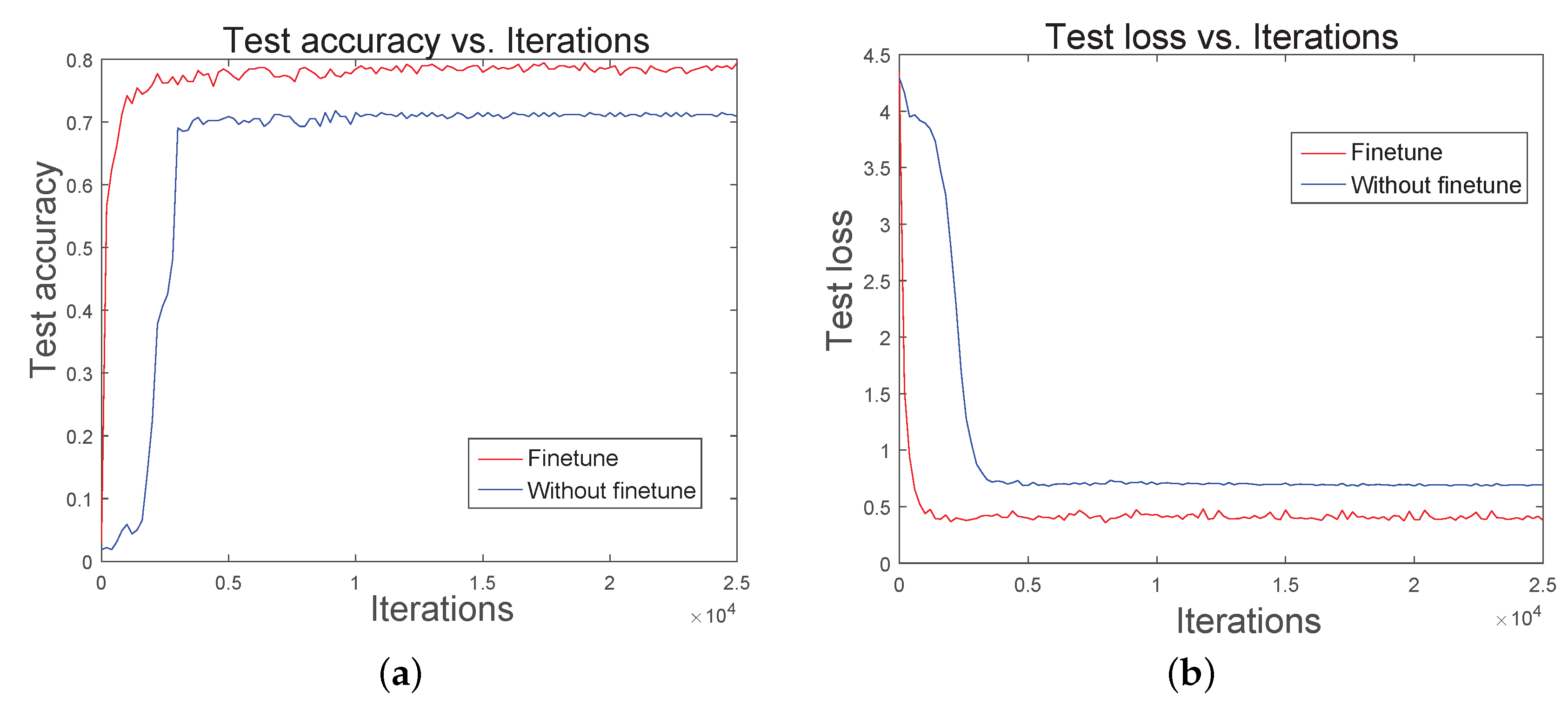
To get better results with less time, fine-tuning is used in the training process. Instead of training a CNN from scratch, a pretrained VGG-16 model for face recognition on the VGG-Face dataset is used. Fine-tuning is then used to refine the weights. Before fine-tuning the VGG-16 model, we keep the weights before the fully connected layers fixed, i.e., weights obtained in pretraining. The weights of the fully connected layer are initialized from zero mean Gaussian distribution with standard deviation of 0.01. As shown in Figure 5, we fine-tune the VGG-16 network; the accuracy of the model without fine-tuning is 70.4%, whereas with fine-tuning 79.6%. Additionally, the model with fine-tuning achieves a higher accuracy with fewer iterations. Thus, fine-tuning can improve the efficiency of training and get a better result with fewer iterations.

In our experiment, different data augmentation methods are used to enlarge the number of original training samples for fine-tuning the CNN model. To verify the effectiveness of our CNN model, which is based on the augmented training samples, our methods are compared with traditional face recognition methods such as PCA and LBPH. PCA is often used to reduce the dimensionality of datasets while keeping the values which contribute most to variance. It decomposes the covariance matrix to obtain the principal components (i.e., eigenvector) of the data and their corresponding eigenvalues. The LBPH method is based on the Local Binary Patterns (LBP), which is proposed as a texture description method. For texture classification, the occurrences of the LBP codes in a face image are collected into a histogram. The classification is then performed by computing the similarity between histograms. In terms of the accuracy for face recognition, our methods are better than the PCA and LBPH methods (see

Table 4. Recognition performance with different methods.

Method	Accuracy
PCA method	(18/54) 33.3%
LBPH method	(19/54) 35.2%
CNN with geometric transformation and brightness augmentation method	(45/54) 83.3%
CNN with filter operation augmentation method	(41/54) 75.9%

). The experimental results show the effectiveness of the prediction approach with various virtual samples. This approach is an effective and robust method for class attendance taking. In terms of face recognition with a small number of samples, our method using CNN with data augmentation has more advantages than that of the PCA and LBPH methods. However, there are still some drawbacks compared with other CNN models. Our dataset is small and acquired in a natural uncontrolled environment, whereas nearly all of the state-of-the-art approaches are developed using large datasets acquired in well-controlled environments. The quality of our training samples is lower than that of standard face datasets. First, compared with other data-driven based methods, the number of our training images is still insufficient. Second, only a single viewpoint is available in our original training samples. Third, some students may be occluded by others in the photos.

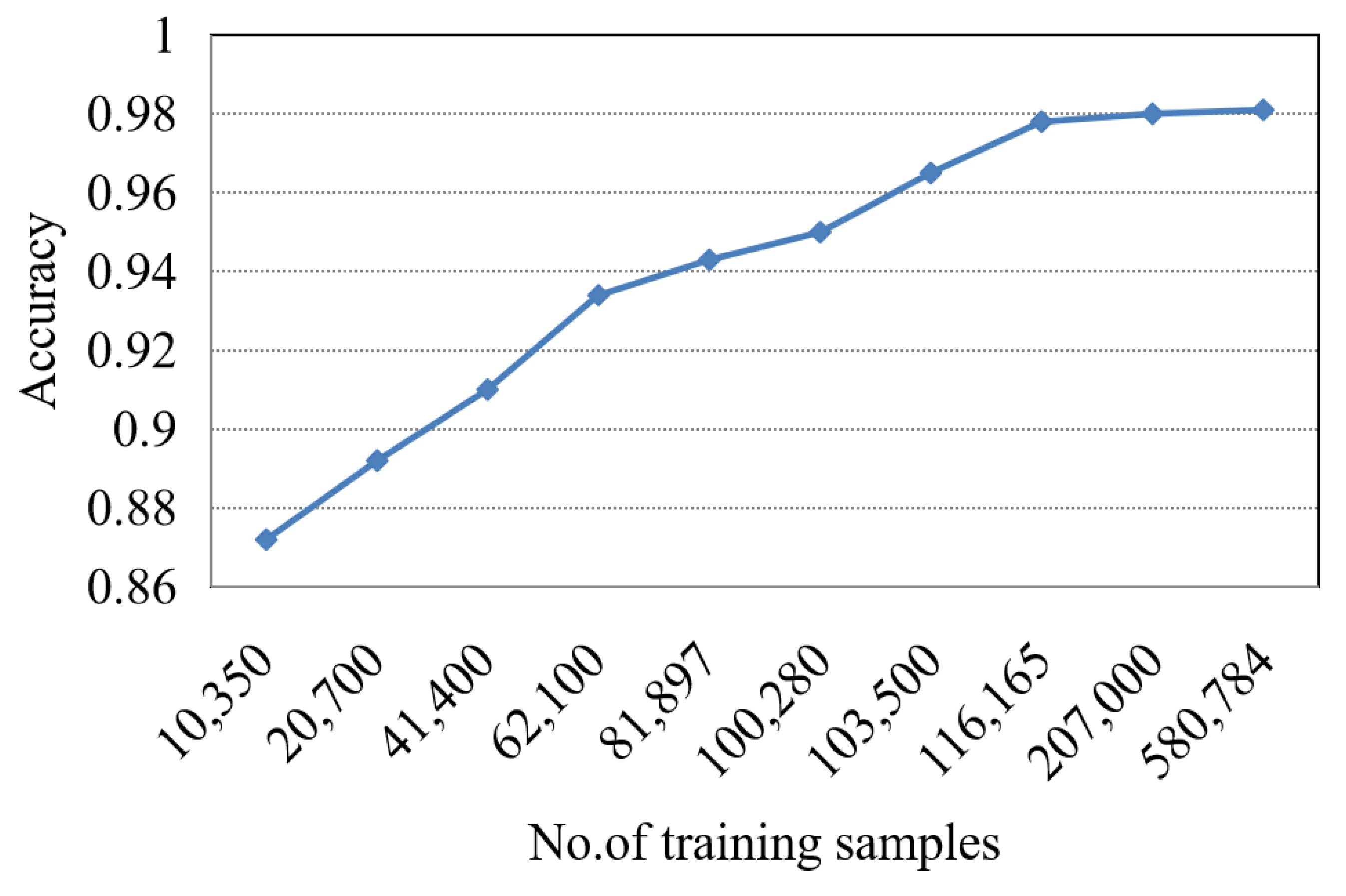
We also investigate the relationship between the quantity of training samples and the recognition accuracy in a class. In particular, we take videos of students in a classroom, and each video is approximately two minutes. During the video taking process, we instruct the students to change their expressions and head postures to enrich variations in the facial samples. Later, the AdaBoost algorithm is used to extract students’ faces from each frame in the video to update the dataset. Finally, we choose a different number of training samples for the experiments with VGG-16. Additionally, the best data augmentation method is used in the last three experiments. As shown in Figure 6, the more training samples are used for fine-tuning, the higher the accuracy and performance of the model is. Additionally, with 0.11 million samples, the accuracy can achieve an accuracy of 98.1%. This indicates that if the instructor can take videos in the first few classes, the number of training samples for each student can increase substantially, and therefore can improve the recognition performance significantly for the rest of the term.

6. Conclusions

In this paper, we propose a novel method for class attendance taking using a CNN-based face recognition system. To acquire enough training samples, we analyze different data augmentation methods based on the orthogonal experiments. According to the orthogonal table, the best data augmentation method can be determined. Then, we demonstrate that the CNN-based face recognition system with data augmentation can become an effective method with sufficient accuracy of recognition. The experimental results indicate that our method can achieve an accuracy of 86.3%, which is higher than PCA or LBPH method. If videos could be taken during the first few classes, the accuracy of our method could reach 98.1%.

References

- Louis, W.R.; Bastian, B.; McKimmie, B.; Lee, A.J. Teaching psychology in A ustralia: Does class attendance matter for performance? Aust. J. Psychol. 2016, 68, 47–51. [Google Scholar] [CrossRef]
- Pss, S.; Bhaskar, M. RFID and pose invariant face verification based automated classroom attendance system. In Proceedings of the 2016 International Conference on Microelectronics, Computing and Communications (MicroCom), Durgapur, India, 23–25 January 2016; pp. 1–6. [Google Scholar] [CrossRef]
- Apoorv, R.; Mathur, P. Smart attendance management using Bluetooth Low Energy and Android. In Proceedings of the 2016 IEEE Region 10 Conference (TENCON), Singapore, 22–25 November 2016; pp. 1048–1052. [Google Scholar] [CrossRef]
- Kohana, M.; Okamoto, S. A Location-Based Attendance Confirming System. In Proceedings of the 2016 IEEE 30th International Conference on Advanced Information Networking and Applications (AINA), Crans-Montana, Switzerland, 23–25 March 2016; pp. 816–820. [Google Scholar]
- Dhanalakshmi, N.; Kumar, S.G.; Sai, Y.P. Aadhaar based biometric attendance system using wireless fingerprint terminals. In Proceedings of the 2017 IEEE 7th International Advance Computing Conference (IACC), Hyderabad, India, 5–7 January 2017; pp. 651–655. [Google Scholar]
- Soewito, B.; Gaol, F.L.; Simanjuntak, E.; Gunawan, F.E. Smart mobile attendance system using voice recognition and fingerprint on smartphone. In Proceedings of the 2016 International Seminar on Intelligent Technology and Its Applications (ISITIA), Lombok, Indonesia, 28–30 July 2016; pp. 175–180. [Google Scholar] [CrossRef]
- Lukas, S.; Mitra, A.R.; Desanti, R.I.; Krisnadi, D. Student attendance system in classroom using face recognition technique. In Proceedings of the 2016 IEEE International Conference on Information and Communication Technology Convergence (ICTC), Jeju, Korea, 19–21 October 2016; pp. 1032–1035. [Google Scholar] [CrossRef]
- Devan, P.A.M.; Venkateshan, M.; Vignesh, A.; Karthikraj, S. Smart attendance system using face recognition. Adv. Natural Appl. Sci. 2017, 11, 139–145. [Google Scholar]
- Rekha, E.; Ramaprasad, P. An efficient automated attendance management system based on Eigen Face recognition. In Proceedings of the 2017 IEEE 7th International Conference on Cloud Computing, Data Science & Engineering-Confluence, Noida, India, 12–13 January 2017; pp. 605–608. [Google Scholar] [CrossRef]
- Sahani, M.; Subudhi, S.; Mohanty, M.N. Design of Face Recognition based Embedded Home Security System. KSII Trans. Internet Inf. Syst. 2016, 10. [Google Scholar] [CrossRef]
- Ramkumar, M.; Sivaraman, R.; Veeramuthu, A. An efficient and fast IBR based security using face recognition algorithm. In Proceedings of the 2015 IEEE International Conference on Communications and Signal Processing (ICCSP), Melmaruvathur, India, 2–4 April 2015; pp. 1598–1602. [Google Scholar] [CrossRef]
- Xu, W.; Shen, Y.; Bergmann, N.; Hu, W. Sensor-assisted multi-view face recognition system on smart glass. IEEE Trans. Mob. Comput. 2017, 17, 197–210. [Google Scholar] [CrossRef]
- Shin, Y.; Balasingham, I. Comparison of hand-craft feature based SVM and CNN based deep learning framework for automatic polyp classification. In Proceedings of the 2017 39th Annual International Conference of the IEEE Engineering in Medicine and Biology Society (EMBC), Jeju Island, Korea, 11–15 July 2017; pp. 3277–3280. [Google Scholar] [CrossRef]
- Taigman, Y.; Yang, M.; Ranzato, M.; Wolf, L. Deepface: Closing the gap to human-level performance in face verification. In Proceedings of the IEEE Conference on Computer Vision and Pattern Recognition, Columbus, OH, USA, 23–28 June 2014; pp. 1701–1708. [Google Scholar]
- Schroff, F.; Kalenichenko, D.; Philbin, J. Facenet: A unified embedding for face recognition and clustering. In Proceedings of the IEEE Conference on Computer Vision and Pattern Recognition, Boston, MA, USA, 7–12 June 2015; pp. 815–823. [Google Scholar] [CrossRef]
- Liu, W.; Wen, Y.; Yu, Z.; Li, M.; Raj, B.; Song, L. Sphereface: Deep hypersphere embedding for face recognition. In Proceedings of the IEEE Conference on Computer Vision and Pattern Recognition, Honolulu, HI, USA, 22–25 July 2017; pp. 212–220. [Google Scholar]
- Deng, J.; Guo, J.; Xue, N.; Zafeiriou, S. Arcface: Additive angular margin loss for deep face recognition. In Proceedings of the IEEE Conference on Computer Vision and Pattern Recognition, Long Beach, CA, USA, 16–20 June 2019; pp. 4690–4699. [Google Scholar] [CrossRef]
- Kim, D.; Hernandez, M.; Choi, J.; Medioni, G. Deep 3D face identification. In Proceedings of the 2017 IEEE International Joint Conference on Biometrics (IJCB), Denver, CO, USA, 1–4 October 2017; pp. 133–142. [Google Scholar] [CrossRef]
- Tornincasa, S.; Vezzetti, E.; Moos, S.; Violante, M.G.; Marcolin, F.; Dagnes, N.; Ulrich, L.; Tregnaghi, G.F. 3D Facial Action Units and Expression Recognition using a Crisp Logic. Comput. Aided Des. Appl. 2019, 16, 256–268. [Google Scholar] [CrossRef]
- Dagnes, N.; Marcolin, F.; Vezzetti, E.; Sarhan, F.R.; Dakpé, S.; Marin, F.; Nonis, F.; Mansour, K.B. Optimal marker set assessment for motion capture of 3D mimic facial movements. J. Biomech. 2019, 93, 86–93. [Google Scholar] [CrossRef] [PubMed]
- Salamon, J.; Bello, J.P. Deep convolutional neural networks and data augmentation for environmental sound classification. IEEE Signal Process. Lett. 2017, 24, 279–283. [Google Scholar] [CrossRef]
- Okafor, E.; Smit, R.; Schomaker, L.; Wiering, M. Operational data augmentation in classifying single aerial images of animals. In Proceedings of the 2017 IEEE International Conference on INnovations in Intelligent SysTems and Applications (INISTA), Gdynia, Poland, 3–5 July 2017; pp. 354–360. [Google Scholar] [CrossRef]
- Mittal, Y.; Varshney, A.; Aggarwal, P.; Matani, K.; Mittal, V.K. Fingerprint biometric based access control and classroom attendance management system. In Proceedings of the 2015 Annual IEEE India Conference (INDICON), Jamia Millia Islamia, New Delhi, India, 17–19 December 2015; pp. 1–6. [Google Scholar] [CrossRef]
- Nguyen, H.; Chew, M. RFID-based attendance management system. In Proceedings of the 2017 2nd Workshop on Recent Trends in Telecommunications Research (RTTR), Auckland, New Zealand, 10 February 2017; pp. 1–6. [Google Scholar]
- Čisar, S.M.; Pinter, R.; Vojnić, V.; Tumbas, V.; Čisar, P. Smartphone application for tracking students’ class attendance. In Proceedings of the 2016 IEEE 14th International Symposium on Intelligent Systems and Informatics (SISY), Subotica, Serbia, 29–31 August 2016; pp. 227–232. [Google Scholar] [CrossRef]
- Allen, C.; Harfield, A. Authenticating physical location using QR codes and network latency. In Proceedings of the 2017 14th International Joint Conference on Computer Science and Software Engineering (JCSSE), Nakhon Si Thammarat, Thailand, 12–14 July 2017; pp. 1–6. [Google Scholar] [CrossRef]
- Rathod, H.; Ware, Y.; Sane, S.; Raulo, S.; Pakhare, V.; Rizvi, I.A. Automated attendance system using machine learning approach. In Proceedings of the 2017 International Conference on Nascent Technologies in Engineering (ICNTE), Navi Mumbai, Maharashtra, India, 9–10 January 2017; pp. 1–5. [Google Scholar] [CrossRef]
- Wei, X.Y.; Yang, Z.Q. Mining in-class social networks for large-scale pedagogical analysis. In Proceedings of the 20th ACM international conference on Multimedia, Nara, Japan, 29 October–2 November 2012; pp. 639–648. [Google Scholar] [CrossRef]
- Qian, Y.; Gong, M.; Cheng, L. Stocs: An efficient self-tuning multiclass classification approach. In Proceedings of the Canadian Conference on Artificial Intelligence, Halifax, NS, Canada, 2–5 June 2015; pp. 291–306. [Google Scholar] [CrossRef]
- Wu, Z.; Peng, M.; Chen, T. Thermal face recognition using convolutional neural network. In Proceedings of the 2016 International Conference on Optoelectronics and Image Processing (ICOIP), Warsaw, Poland, 10–12 June 2016; pp. 6–9. [Google Scholar] [CrossRef]
- Sun, Y.; Wang, X.; Tang, X. Deep learning face representation from predicting 10,000 classes. In Proceedings of the IEEE Conference on Computer Vision and Pattern Recognition, Columbus, OH, USA, 23–28 June 2014; pp. 1891–1898. [Google Scholar]
- Sun, Y.; Chen, Y.; Wang, X.; Tang, X. Deep learning face representation by joint identification-verification. In Proceedings of the 27th International Conference on Neural Information Processing Systems, Montreal, QC, Canada, 8–13 December 2014; pp. 1988–1996. [Google Scholar]
- Sun, Y.; Wang, X.; Tang, X. Deeply learned face representations are sparse, selective, and robust. In Proceedings of the IEEE Conference on Computer Vision and Pattern Recognition, Boston, MA, USA, 7–12 June 2015; pp. 2892–2900. [Google Scholar] [CrossRef]
- Simonyan, K.; Zisserman, A. Very deep convolutional networks for large-scale image recognition. arXiv 2014, arXiv:1409.1556. [Google Scholar]
- Pei, Z.; Zhang, Y.; Lin, Z.; Zhou, H.; Wang, H. A method of image processing algorithm evaluation based on orthogonal experimental design. In Proceedings of the 2009 Fifth International Conference on Image and Graphics, Xi’an, China, 20–23 September 2009; pp. 629–633. [Google Scholar]
- Ouyang, W.; Wang, X.; Zhang, C.; Yang, X. Factors in fine-tuning deep model for object detection with long-tail distribution. In Proceedings of the IEEE Conference on Computer Vision and Pattern Recognition, Las Vegas, NV, USA, 27–30 June 2016; pp. 864–873. [Google Scholar]
- Jia, Y.; Shelhamer, E.; Donahue, J.; Karayev, S.; Long, J.; Girshick, R.; Guadarrama, S.; Darrell, T. Caffe: Convolutional architecture for fast feature embedding. In Proceedings of the 22nd ACM International Conference on Multimedia, Orlando, FL, USA, 3–7 November 2014; pp. 675–678. [Google Scholar]
- Ji, S.; Lu, X.; Xu, Q. A fast face detection method combining skin color feature and adaboost. In Proceedings of the 2014 International Conference on Multisensor Fusion and Information Integration for Intelligent Systems (MFI), Beijing, China, 28–29 September 2014; pp. 1–5. [Google Scholar] [CrossRef]
Figure 1.
An illustration of the architecture of the VGG-16 model.
Figure 2.
The workflow of our class attendance-taking method. First, the instructor takes a photo of the class with all the students’ faces. Then, face detection is used to capture each student’s face. Data augmentation is performed to increase the number of training images in the dataset. Finally, the convolutional neural network (CNN) can be trained to generate a model that can be used to predict a student’s name.
Figure 3.
Geometric transformation and image brightness manipulation. (a) The original face image. (b) Result of image translation. (c) Result of image rotation. (d) Result of image zoom. (e) Result of changes of image brightness.
Figure 4.
Filter operation. (a) The original face image. (b) Result of using a mean filter. (c) Result of using a median filter. (d) Result of using a Gaussian filter. (e) Result of using a bilateral filter.
Figure 5.
Training the model with different initialization methods. (a) Accuracy vs. Iterations on the CNN architecture. (b) Test loss vs. Iterations on the CNN architecture.
Figure 6.
The recognition performance of different number of training samples.