A Highly Relevant Method for Incorporation of Shunt Connected FACTS Device into Multi-Machine Power System to Dampen Electromechanical Oscillations


1
Institute of Research and Development, Duy Tan University, Da Nang 550000, Vietnam
2
Faculty of Electricity Engineering, Industrial University of Ho Chi Minh City, Ho Chi Minh City 700000, Vietnam
3
Department of Engineering and Technology, Quy Nhon University, Binh Dinh 820000, Vietnam
4
Department for Management of Science and Technology Development, Ton Duc Thang University, Ho Chi Minh City 700000, Vietnam
5
Faculty of Electrical & Electronics Engineering, Ton Duc Thang University, Ho Chi Minh City 700000, Vietnam
*
Author to whom correspondence should be addressed.
Energies 2017, 10(4), 482; https://doi.org/10.3390/en10040482
Submission received: 18 January 2017
/
Revised: 26 March 2017
/
Accepted: 29 March 2017
/
Published: 4 April 2017
(This article belongs to the Special Issue Electric Power Systems Research 2017)
Abstract
:A number of techniques have been proposed to dampen the power system oscillations in the electric power systems. Flexible alternating current transmission system (FACTS) devices are becoming one of them. Among the FACTS family, the static synchronous compensator (STATCOM), a shunt connected FACTS device, has been widely used to provide smooth and rapid steady state, limit transient voltage, and improve the power system stability and performance by absorbing or injecting reactive power. However, the influence ability depends on its placement, control signal, and place of receiving-signal in the network. In order to satisfy these issues, this paper proposes a method for optimal setting and signal position of the STATCOM into the multi-machine power systems with the aim for damping the electromechanical oscillations. This method is developed from the energy approach based on Gramian matrices considering multiple tasks on the Lyapunov equation, in which the observability Gramian matrix is used to seek an optimal location for STATCOM placement. The another is the controllability one used to determine the best local input signal placement that is chosen as a feedback signal for the power oscillation damping (POD) of STATCOM. In addition, the Krylov-based model reduction method is introduced to shorten the calculation time. The proposed method has been verified on the IEEE 24-bus system by analyzing the small-signal stability to search several feasible placements, and then the transient stability is analyzed to compare and determine an optimal placement through testing various cases. The obtained result is also compared with other optimal method.
1. Introduction
In recent years, the demand of electrical power increases due to the social, political, and technological perspective. The distributed generators (DGs) and renewable energy generation have become an inevitable trend because of the economic, environmental, and critical factors and limiting available primary energy resources. When they are connected into the existing power system far away from the load centers, leading on an increase in the scale and complexity of the electric power systems, most power systems operate with requirement very close to their limits and always constrained by small-signal and transient stability conditions. If the inertial response and power damping capability are an insufficient quality when disturbances in the power system occur, low frequency oscillations may appear. These oscillations are due to the outcome of dynamical coactions between the generators within a system. Thus, it can lead to the generators outage, lines tripping, and regions blackout of the system.
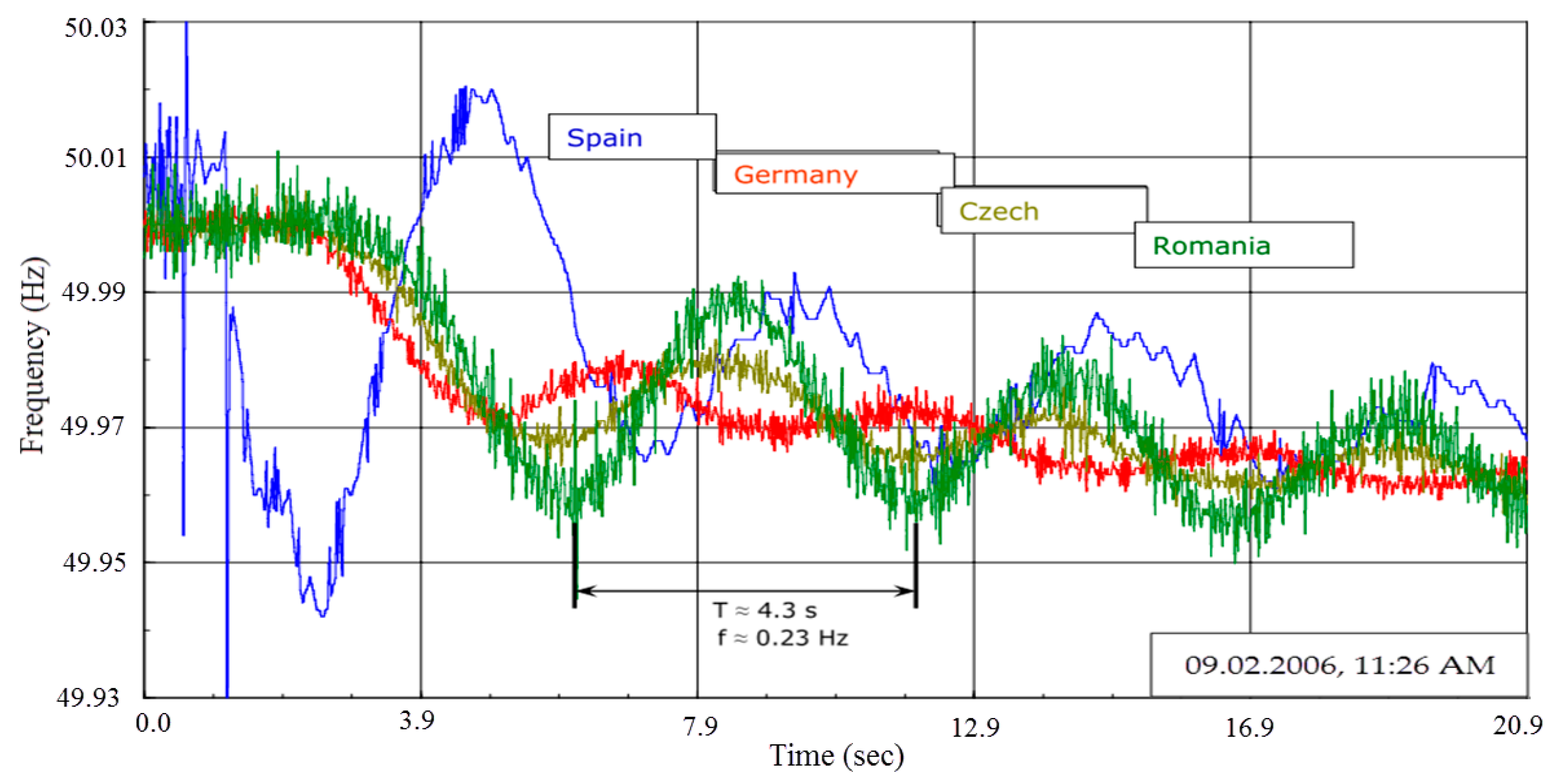
In the past five decades, the power systems around the world have faced more blackouts with various severities due to human and technical faults. Power-technology.com has listed out the world’s top 10 worst blackouts, such as Indian on 30 and 31 July 2012; Paraguay-Brazil on 10 November 2009; Chenzhou in China in January and February 2008; Germany, France, Italy and Spain on November 2006; Indonesia on 18 August 2005; Greece on 12 July 2004; Switzerland on 28 September 2003; Eight U.S. states and Canada on 14 August 2003; Quebec and parts of the U.S. on March 1989; New York City on 13 July 1977; and USA on 9 November 1965, all of which have happened in the last 50 years. Among them, the Indian grid disturbance is a notable event, leaving 620 and 370 million people without electric power for several hours on two days, 30 and 31 July 2012, respectively. The least event is the power system blackout in South Australia on 28 September 2016. Figure 1 is an example of the instable inter-area event of recording a wide area measuring system (WAMS) on 9 February 2006 in Spain [1]. Clearly, observing from this figure, it can be shown significant changes of the dynamic behavior of the system due to the loss of generated power 1.2 GW. The frequency decreases immediately in the proximity of one of power plant outage. The decrease of frequency spreads over the whole system and finally reaches the Romania system with a time delay of about 2.0 s. This event tells us that the inter-area oscillations have a frequency range 0.21–0.25 Hz.
The low frequency electromechanical oscillations happen in the power systems due to the contingencies. These oscillations have a frequency range 0.1–2.0 Hz, classified into two groups based on the energy of oscillation: (i) occurring between generators in a small group, called local mode, having a frequency range 0.7–2.0 Hz; and (ii) occurring between generators in large groups, called inter-area oscillations, having a frequency range 0.1–0.8 Hz [2,3]. Such oscillations menace the stability point of the power system, thus damping these oscillations is necessary for the sure system operation. From the viewpoint of the system instability due to the limited value increment for current network structure, accordingly, most of the efforts for damping oscillations focus on using the controllers to improve the oscillation damping ability, such as Flexible alternating current transmission system (FACTS) devices, power system stabilizers (PSSs), energy storage systems (ESSs), and so on. The installation of PSS in the system is the traditional method. For this method, the adverse effects are the local-area mode oscillations damping, the variation in the voltage profile under serious disturbances, the leading power factor [4]. FACTS is widely used to enhance the operational flexible of the system under other operation conditions, and especially to damp out local- and inter-area mode oscillations [5,6]. This device has the ability to control the parameters of the power system or to modify the load flow, so that the power system may be improved stability and damped oscillations when the grid faults occurred. Thus, FACTS could be the best alternative to enhance the stability margin of the existing power systems and it provides against the inter-area oscillation damping better than PSSs [7]. For ESS device, from the point of view of the power system control, the ESSs are better than the FACTS and PSSs, because they cannot only regulate the reactive power exchange but also the active power with the power system where it is installed. The purpose of applying ESS technology in power is the same FACTS and PSS. However, in order to enhance the power system oscillation damping, ESSs are more flexible than PSSs [8] because of exchanging active power directly. For instance, Du et al. [9] have explained why and how the battery energy storage system (BESS) based on stabilizer can dampen the inter-area oscillations in a multi-machine power system. Chen et al. [10] introduced the complex torque coefficient method to analyze the use of the energy storage system ESS based on flywheel storage technology for damping the power system oscillations of the infinite-bus power system considering single-machine. For this paper, we only focus to dampen the power system oscillations using FACTS device. However, the benefits of FACTS depend greatly on their placement in network [2,7,11]. Consequently, the optimal location of FACTS devices, and especially static synchronous compensator (STATCOM) in the multi-machine, is an interesting research topic.
In the last decades, many researchers have proposed techniques for locating the location of FACT based on two groups: (i) analytical methods; and (ii) heuristic optimization approaches [12,13,14]. Methods based on heuristic algorithms include the genetic algorithm (GA) [15], the particle swarm optimization (PSO) technique [16], the cuckoo search algorithm [17], modified artificial bee colony algorithm (MABCA) [18], and simulate annealing (SA) [19]. These methods were used to increase system load-ability and the system security margin. Evolutionary algorithm (EA) [20] and bacterial swarming algorithm (BSA) [21] are used to minimize the real power loss in the transmission lines and to improve voltage profile at load buses. The bees algorithm (BA) is applied by [22] to maximize the available transfer capability of power agreement between sink areas and source. Contrasting to the heuristic methods, some authors proposed the analytical methods. For example, Sadikovic et al., Magaji et al. [23,24] have proposed the residue factor method to damp inter-area mode of oscillations. Kunnar et al. [25] have utilized the modal controllability index to dampen inter-area oscillations. Van Dai et al., Le et al. [2,11], have introduced the energy method to dampen the power system oscillations in IEEE 39-bus power system, and Zamora-Cárdenas et al. [26] proposed the multi-parameter trajectory sensitivity approach to determine the optimal placement of series FACTS devices with the objective of providing enough level of transient stability.
In addition, the optimal location of STATCOM highly depends on the supplemental controller, namely the power oscillation damping (POD) controller and its feedback signal position [27]. Leading in recent years, many of the optimization methods have been proposed to find out ways for answering the question of which POD controller and its feedback signal could result in the STATCOM having the considerable effect on the system. For example, genetic algorithm (GA) is proposed by Eshtehardiha et al., Panda et al. [28,29], but this method requires a very long run time to the large-scale systems. Safari et al. [30] introduced the Artificial Bee Colony (ABC) method, but the convergence is very slow. Abd-Elazim et al. [31] introduced the imperialist competitive algorithm (ICA) for optimal design of STATCOM parameters. In addition, local input signals as the line reactive and active power, line current, and bus voltage are all good selections for the feedback signal of POD controller of FACTS to dampen the power system oscillations [2,11]. The active power in the transmission line is considered as an effective input signal for POD controller [32]. Reference [33] concluded that the current or active power is not difference when using them as the feedback signal. For this paper, the active power in the transmission line is chosen as a feedback signal. However, in the previous proposed researches, the authors did not mention the location of input signal placement.
It can be observed that most employed techniques in the previous literature have several drawbacks: (i) There is no mention of the optimal location of the local input signal for the POD of STATCOM; (ii) Slow convergence in search stage, limit of local search ability, and the requested process time is very long when studying the large-scale systems, so they just focus on analyzing the small-scale power systems; (iii) The calculation of critical modes may be doubtful in the case of the larger-scale and complex power systems because they may not be unique. Furthermore, the calculation of these critical modes also depends on the local- or inter-area mode; (iv) The calculation of participation coefficients is only based on the state variables and neglects the input–output behaviors. Therefore, in order to overcome these drawbacks, this paper proposes a feasible method. This method is a conjunction between the energy method based on the observability and controllability Gramian matrices and the Krylov-based model reduction method to determine the optimal location of STATCOM and the local input signal position of POD controller with aim of improving the stability of the large-scale power systems, respectively.
The main contribution of this paper is to propose a feasible method:
- (i)
- To determine the optimal placement of STATCOM and the best local input signal position of its POD controller;
- (ii)
- To limit the time calculation when analyzing the complexity and large-scale power systems on the small-signal stability analysis.
The remainder of this paper is organized as follows: Section 2 analyzes the mathematical model of the STATCOM, power system, and incorporation the STATCOM in the power system. Section 3 explains the methods for designing POD of STATCOM and selecting the location of STATCOM-POD and location of the feedback. The details of the test cases are given in Section 4. Finally, the conclusion is outlined in Section 5 and the Arnoldi algorithm, QR decomposition, and parameters of the STATCOM are detailed in Appendix A.
2. Analysis of Mathematical Models
2.1. STATCOM Model
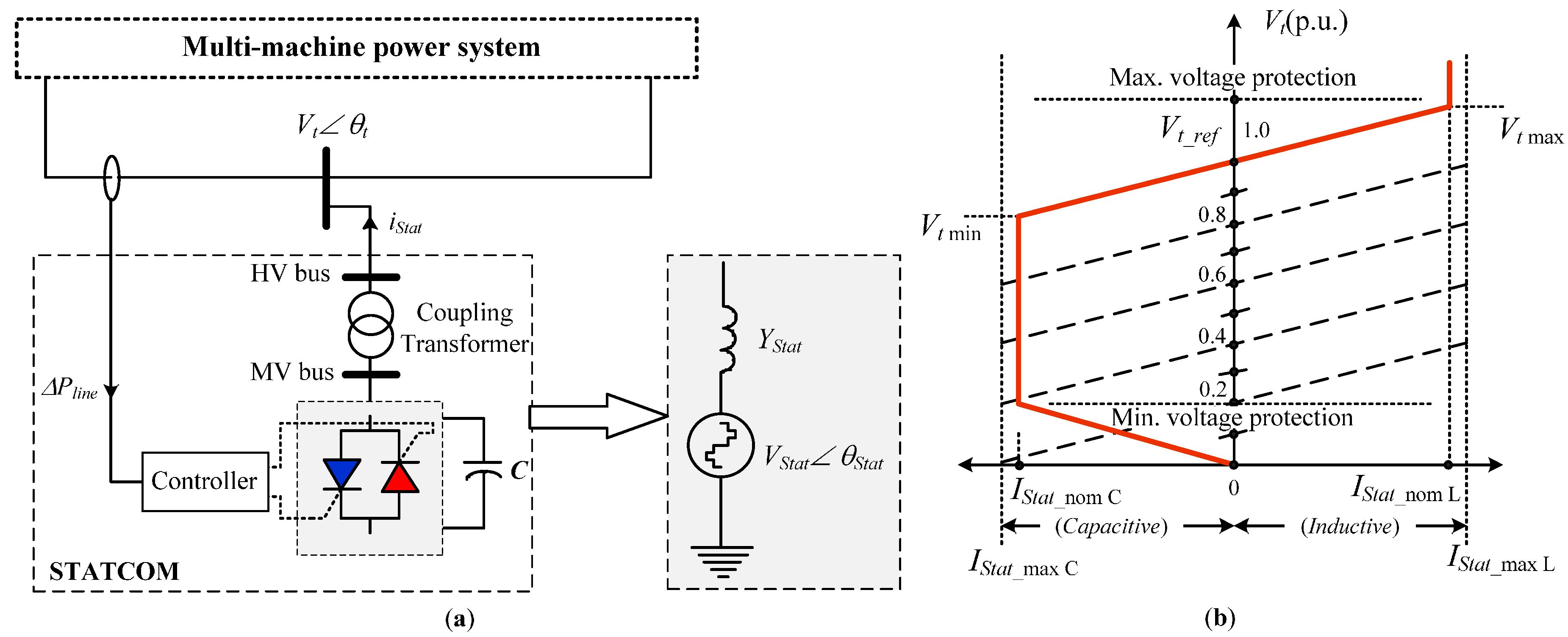
The STATCOM is one the most noteworthy series of the FACTS derives. The main function of STATCOM is to control a fast response of the transmission voltage, increase the power transfer on transmission line, and improve the transient stability of the power network by generating and/or absorbing reactive power after clearing fault. In this paper, the structure of a STATCOM consisting of a voltage source converter (VSC), a coupling transformer, a DC capacitor, and controller unit is used to study, as shown in Figure 2a. Its operational Voltage–Current characteristic is shown in Figure 2b.
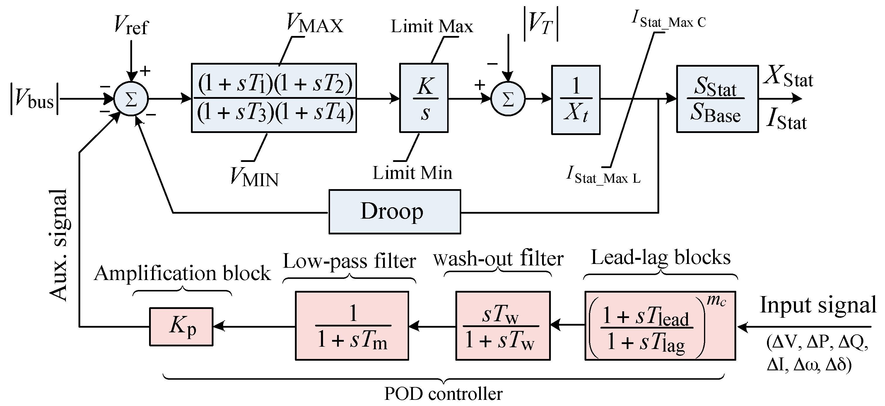
The objective of this paper is to investigate the damping of power system oscillations when the grid fault occurs, STATCOM should operate over the rated maximum inductive and/or capacitive compensation range being independent of the AC system voltage. Accordingly, the controller is designed to control STATCOM, so that it always keeps full capability during most severe contingencies. The output current variable can be obtained by using various control approaches. Besides, this output current variable depends on the position and kind (active power, reactive power, current of transmission line, transmission angle, or generator rotor speed) of the feedback signal. For this purpose, the dynamic model is proposed for STATCOM [34]. This dynamic mode is compound of the voltage regulator with transient gain, and can be determined by the time constants T1 through T4 and integrator K. The steady-state gain is equal to the inverse of Droop, which allows the sharing of voltage of generators. The inputs to model are the monitored voltage Vbus, voltage reference on the connected STATCOM bus Vref, the STATCOM internal voltage VT, and the auxiliary signal. This auxiliary signal is generated from the power oscillation damping (POD) controller. This POD consists of an amplification block, a wash-out filter, a low-pass filter, and mc stages of lead-lag blocks as shown in Figure 3, where Tm, Tw, Tlead, and Tlag are the measurement, washout, lead, and lag time constants, respectively. The input signal could be the line active and reactive power, current, bus voltage, generator angle speed, or phase angle.
The output current of STATCOM is varied according to firing angle control, which is adjusted through the voltage regulator with transient gain and integrator gain to main the STATCOM bus voltage at the desired reference value. By linearizing the STATCOM dynamic model with POD controller, we can be obtained as follows [35]:
where the matrices AStat and BStat depend on the time constants T1 through T4, gain K, the monitored voltage Vbus, the voltage reference Vref, and the STATCOM internal voltage VT.
2.2. Power System Model
The methodological method of the dynamic modeling of the multi-machine power system with m-machine and n-bus has been described in [36] applied to this case study. In this model, each synchronous generator is represented by two-axis flux decay dynamic and the Excitation system is used the IEEE type I to provide the generator [37]. The differential algebraic equation (DAE) model of the multimachine power system without FACTS can be expressed the following equation:
in which x, y, and u are the state, algebraic, and input vectors, respectively and are defined as:
where
| the transpose operator; | |
| the rotor angle of generator ith; | |
| the speed of generator ith; | |
| the voltage magnitude at bus jth; | |
| the phase angle at bus jth; | |
| the d-axis component of the current of generator ith; | |
| the q-axis component of the current of generator ith; | |
| the input amplifier voltage the excitation of generator ith; | |
| the stabilizer feedback variable of the excitation of generator ith; | |
| the electrical power of generator ith; | |
| the q-axis component of the internal voltage of generator ith; | |
| the d-axis component of the internal voltage of generator ith; | |
| the d-axis component of the field voltages of generator ith; and | |
| the reference voltage of generator ith. |
According to the methodology presented in [36], the linearized model is considered and given the following symbolic form:
Equation (4) can be rewritten as:
where A’, B’, C’, D’, and E’ are appropriate Jacobians of the system in Equation (2) evaluated at the operating point, and can identify as follows:
and
Therefore, this methodology utilized to analyze the small-signal stability programs using PSS/E (Power System Simulator for Engineering) and Matlab softwares.
2.3. The STATCOM-Power System Model
The STATCOM can be installed at the existing load bus or the extra bus that created between two the existing buses of the multimachine power system. As such, in this case study, a STATCOM is installed at the bus t in the n-bus power system, the injected power flow into the bus t are given the following equations [38]:
where PStat and QStat are, respectively, the active and reactive power at converter terminal at the bus t, that are:
in which Vt, θt, Vk, θk, VStat and θStat are the voltage magnitudes and phase angles at bus t, k, and converter terminal, respectively; and Yt = Gt + jBt, Ytk = Gtk + jBtk, and YStat = GStat + jBStat are the values of self-admittance at bus t for the existing n-bus power system, between buses t and k, and converter terminal, respectively.
Linearizing Equation (8) and combining Equation (1), the linearized model of STATCOM can be derived as the following equation:
where AStat, BStat, CStat, and DStat are appropriate Jacobians of the system in Equation (8) evaluated at the operating point; the voltage magnitude VStat and phase angle θStat at converter terminal are considered as state variables [38].
The methodology for incorporating FACTS devices into the n-bus power system is developed [35,36,38,39,40]. Based on this methodology, the DAE model of m-machine and n-bus power system with the STATCOM can be obtained by combining Equations (5) and (10):
Equation (11) can be rewritten as:
in which, Anew, Bnew, Cnew, Dnew, and Enew are appropriate Jacobians of the new system evaluated at the operating point, and can identify as follows:
and
The meaning of all state variables in Equation (14) is the same as that in Equation (3), but corresponding to the power system with STATCOM.
3. Methods Analysis
In this section, it elaborates on mathematical steps taken to formulate expressions for finding optimal STATCOM placement. The method based on two controllability and observability properties of the system, playing an important role in determining the location of placement and input signal of STATCOM, is explained. In order to evaluate these controllability and observability indexes, the linear dynamic system will be considered under the state-space form is necessary to detail conjunction between output and input signals, which contain more information about the internal states of system. Based on Equation (12), a linear time invariant system with FACTS except POD controller described in the state-space form as follows:
where
| x(t) | the state vector of length equal to the number of states n; |
| y(t) | the output vector of length equal to the number of output m; |
| u(t) | the input vector of length equal to the number of input r; |
| A | the state matrix of size n × n; |
| B | the control matrix of size n × r; |
| C | the output matrix of size m × n; and |
| D | the feed-forward matrix of size m × r. |
3.1. The Order Reduction Method
For a large-scale power system, the number of state variables could be big, taking a long time to process even when the modern computer systems are used. The small-signal stability analysis only needs to take into account the number of the important state variables, being normally smaller than the number of the state variables of the original linearized power system. In order to solve this problem, the order reduction solutions were studied in [41], in which the Krylov-based model reduction solution is selected and reusable to study, and can be summed up as below.
The transfer function of the system in Equation (15) can be described as follows:
and can be expanded under the Laurent series form around certain point s0
where μ(0, 1, 2, …, k) denotes the moments and the kth moment can be defined as:
it should be noted that the Laurent series expansion can be done around different points.
Expanding the Laurent series in the neighborhood of the arbitrary complex number (s0 ∈ ), the moments are:
If the moments are selected at zero (s0 = 0), the resulting problem is known as Pade approximation, these moments are:
Expanding the Laurent series around infinity (s0 = ), the moments are obtained by deriving from Equations (16) and (18) as:
are called Markov parameters, and the resulting problem is known as partial realization.
In order to solve the above-mentioned model reduction, the algorithm is proposed in [42], namely, the Arnoldi algorithm is reusable. Its procedure is shown in Appendices A.1 and A.2.
After applying the Krylov-based model reduction solution for the original system of large dimension (15), the reduced system obtained as:
As can be observed in Equation (22), the moments of the original and reduced systems equal to the kth term of the Laurent series expansion, and the reduction does not change the inputs and outputs of the original system.
3.2. The Conventional Method
For the purpose of comparison and recognition to the proposed method, an approach, namely the residue method is introduced in [6], again employed in this paper to determine the best siting of STATCOM by tuning parameters of the POD controller. The procedure is re-summed up to suit the objective of this study as follow:
The transfer function of the reduced system in Equation (22) can be described
The transfer function in Equation (23) between the gth output and hth input can be expressed in terms of modes and residues as:
where λi is the ith eigenvalue; ti and υi denote the right and left eigenvectors associated with the ith eigenvalue λi, respectively; N is the total number of eigenvalues; Righ is the residue associated with ith mode and it gives the measure of the sensitivity of mode to a feedback signal between the output gth and input hth; and this Righ can also be expressed in terms of the controllability and observability of mode.
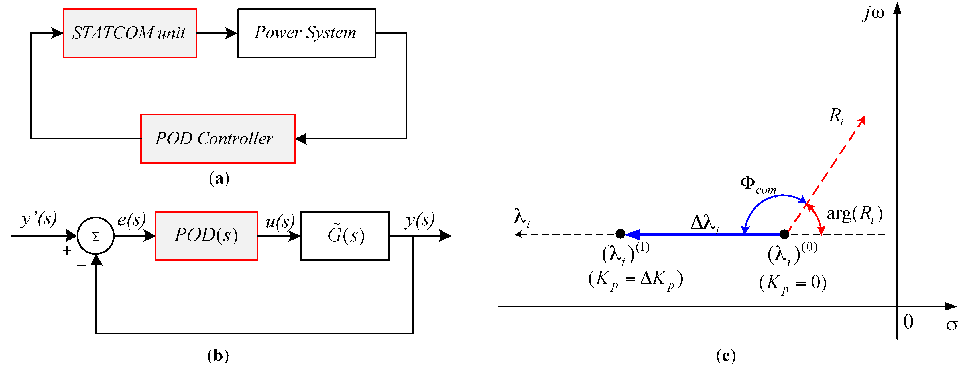
Considering a power system shown in Figure 4a, in which the system includes STATCOM unit and its POD controller. The control close-loop system shown in Figure 4b, where POD(s) is the transfer function of STATCOM-POD controller and is the transfer function of the reduced system. As proposed in this study, POD is a transfer function, as shown in Figure 3, including an amplification block, a wash-out and low-pass filters, and mc stages of lead-lag block, and can be given by:
where Kp is the constant gain. Tm, Tw, Tlead, and Tlag are the measurement, washout, lead, and lag time constants, respectively.
When applying the feedback control, the eigenvalues of the reduced system are changed, so that the eigenvalue sensitivity ith to feedback gain can be calculated as [6,43]:
where Ri denotes the open-loop residue corresponding to eigenvalue ith, λi denotes the mode that should be influenced by the STATCOM damping controller. At the initial operating point that is usually the open-loop system, the eigenvalue λi can be describes under small changes as follows:
and this displacement can show in Figure 4c [6]. It can also be seen in this figure that the angle Φcom is the compensation angle that needs to drive the displacement of eigenvalue. This angle depends on the time constants of the lead-lag function of the POD controller, and these time constants can be calculated by using the following equations:
in which
where ωi is the frequency of the ith oscillation mode, arg(Ri) is the residue phase angle associated with the ith oscillation mode, and mc is the number of compensation stages.
After tuning time constants of the lead-lag, the gain Kp is determined by root-locus method, and it can also calculate this Kp as a function of the desired eigenvalue location based on Equation (27) as follows [6]:
3.3. The Proposed Method
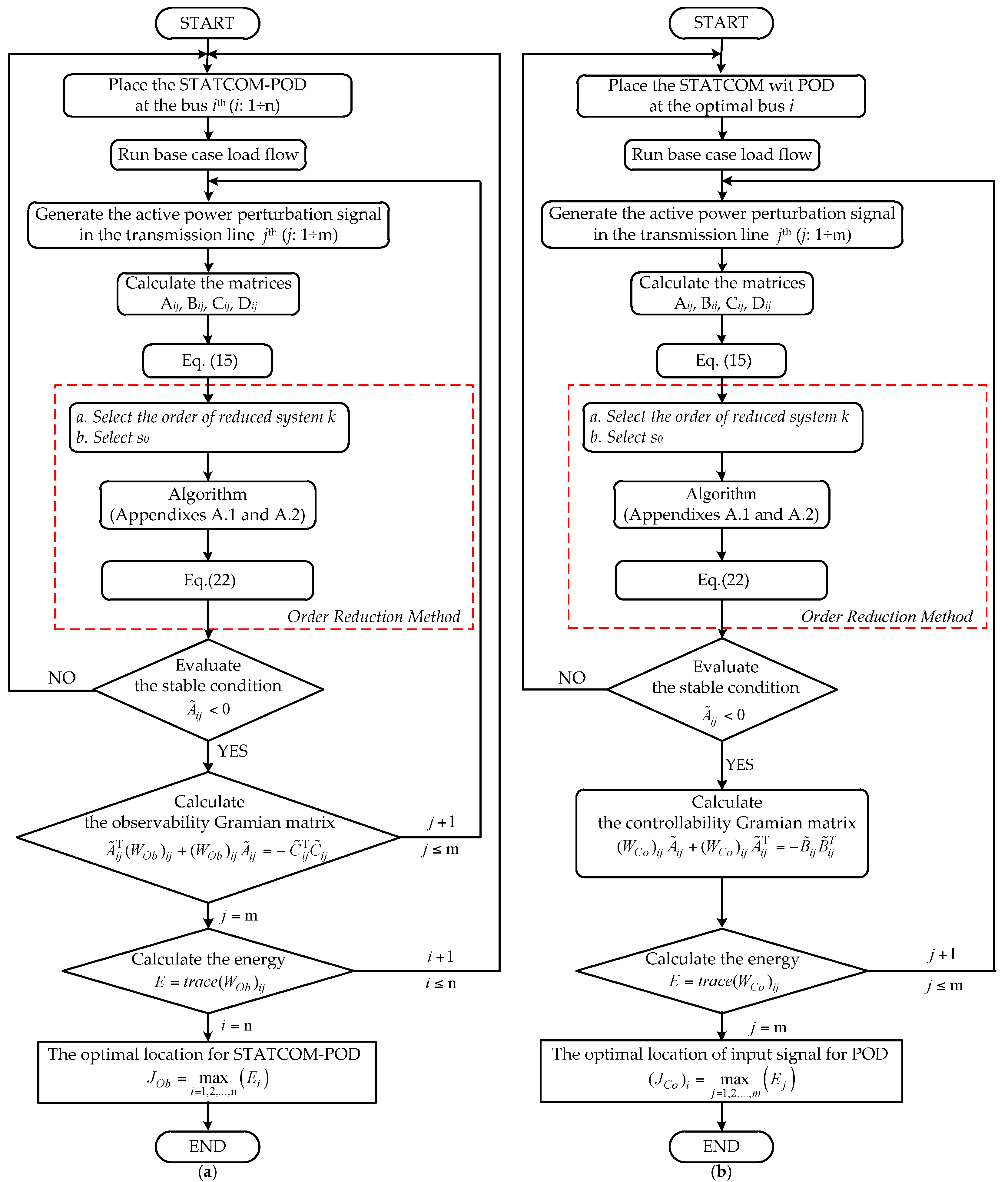
In this section, a method is developed from the Gramian matrix of controllability and observability proposed to determine the optimal location of the sensor (is device using to receive the real power flow from the line and send it to the POD) and STATCOM-POD placements. Two proposed algorithms shown schematically in Figure 5 for these developed applications. Below is the explanation.
3.3.1. Determine Location of Input Signal for POD
The generator speed deviations, bus voltage, real and reactive power flow in the transmission line, and line current are all good nomination in selecting the input signal for the STATCOM control loop [2,11]. The selection of location of these signals placing in the systems with the objective to dampen the power system oscillations is more difficult. In order to solve this problem, a method based on the controllability Gramian matrix of the reduced linearized system is proposed to determine an optimal location for sensor placement. This sensor can receive and send the signal to POD.
For linear time-invariant systems of Equation (22), the observability matrix can be defined as:
and the observability Gramian matrix of the pair () at time t is
can be used to calculate the observability of a system. Therefore, there are two possible ways to check the controllability of a system based on these matrices. Firstly, the pair () is observable if and only if the controllability matrix Co has full rank n, i.e., rank (Co) = n. Secondly, the pair () is controllability if and only if the controllability Gramian matrix WCo(t) is positive definite for t > 0, and it satisfies the following differential Lyapunov matrix equation:
If the system in Equation (22) is asymptotically stable around the origin, then t → , the controllability Gramian matrix can be computed as
and this matrix satisfying the following Lyapunov matrix equation:
Obviously, Equation (35) can see that the observability Gramian matrix WCodepends on the input signal matrix and state matrix ; thus, the input/control energy could be influenced due to these matrixes.
In the case the system is controllable but a transient disturbance occurs, setting up the initial condition x(0) = x0 at time t = 0; it is required to force a final state x1 at final time t1, there exists some input u(t) with t ∈ (−, 0). The amount of energy required to use the input signal for reaching the initial state x0, this energy can be compute as follows [44]:
From Equation (36), the input energy is a quadratic form in the initial state, and it associates with the inverse controllability Gramian matrix. In order to minimize the input/control energy over the entire set, we have to minimize the inverse controllability Gramian matrix or equivalently to maximize controllability Gramian matrix via Trace. Therefore, the optimal location of the sensor can be selected based on the optimization criterion is used as follows:
Figure 5b illustrates the flow chart of calculation steps needed to find the results of optimal location of sensor placement based on the proposed analytical expressions.
3.3.2. Determine Location of STATCOM-POD
As known, the states of a system are internal variables; in a general situation, it cannot to directly measure them, but at the same time, the outputs can be measured quite easily. The observability is the capability of the system to allow the reconstruction of the internal state variables through the time from the measured outputs. Therefore, this property plays an important role in the optimal location analysis of FACTS. Based on this property, a method is developed from the observability Gramian matrix of the reduced linearized system is proposed to determine an optimal location for STATCOM-POD placement.
For linear time invariant systems of Equation (22), the observability matrix can be defined as:
and the observability Gramian matrix of the pair () at time t is
can be used to calculate the observability of a system. Therefore, there are two possible ways to check the observability of a system based on these matrices. Firstly, the pair () is observable if and only if the observable matrix Ob has full rank n, i.e., rank (Ob) = n. Secondly, the pair () is observable if and only if the observability Gramian matrix WOb(t) is positive definite for t > 0, and it satisfies the following differential Lyapunov matrix equation:
If the system in Equation (22) is asymptotically stable around the origin, then t → , the observability Gramian matrix can be calculated:
and it can be satisfied the following Lyapunov matrix equation:
Obviously, Equation (35) can see that the observability Gramian matrix WOb depends only on the output matrix and state matrix . Thus, the output energy could be influenced due to these matrices.
If state x0 ∈ , it exists the outputs y(t): 0 ≤ t < t1, and assuming that the inputs u(t) = 0, are known; this is true, the above system in Equation (22) is observable over the interval [0, t1]. The corresponding output can be computed as follows [45]:
and the output energy at the system is decayed from initial condition x0 to zero in the inexistence of inputs, can be obtained as [44]:
From Equation (44), the output energy is a quadratic form in the initial state, and it associates with the observability Gramian matrix. In order to maximize output energy over the entire set, we have to maximize the observability Gramian matrix via Trace. Therefore, the optimal location of STATCOM-FOD placement can be selected based on the optimization criterion is used as follows:
Figure 5a illustrates the flow chart of calculation steps needed to find the results of optimal location of STATCOM-POD placement based on proposed analytical expressions.
4. Case Study
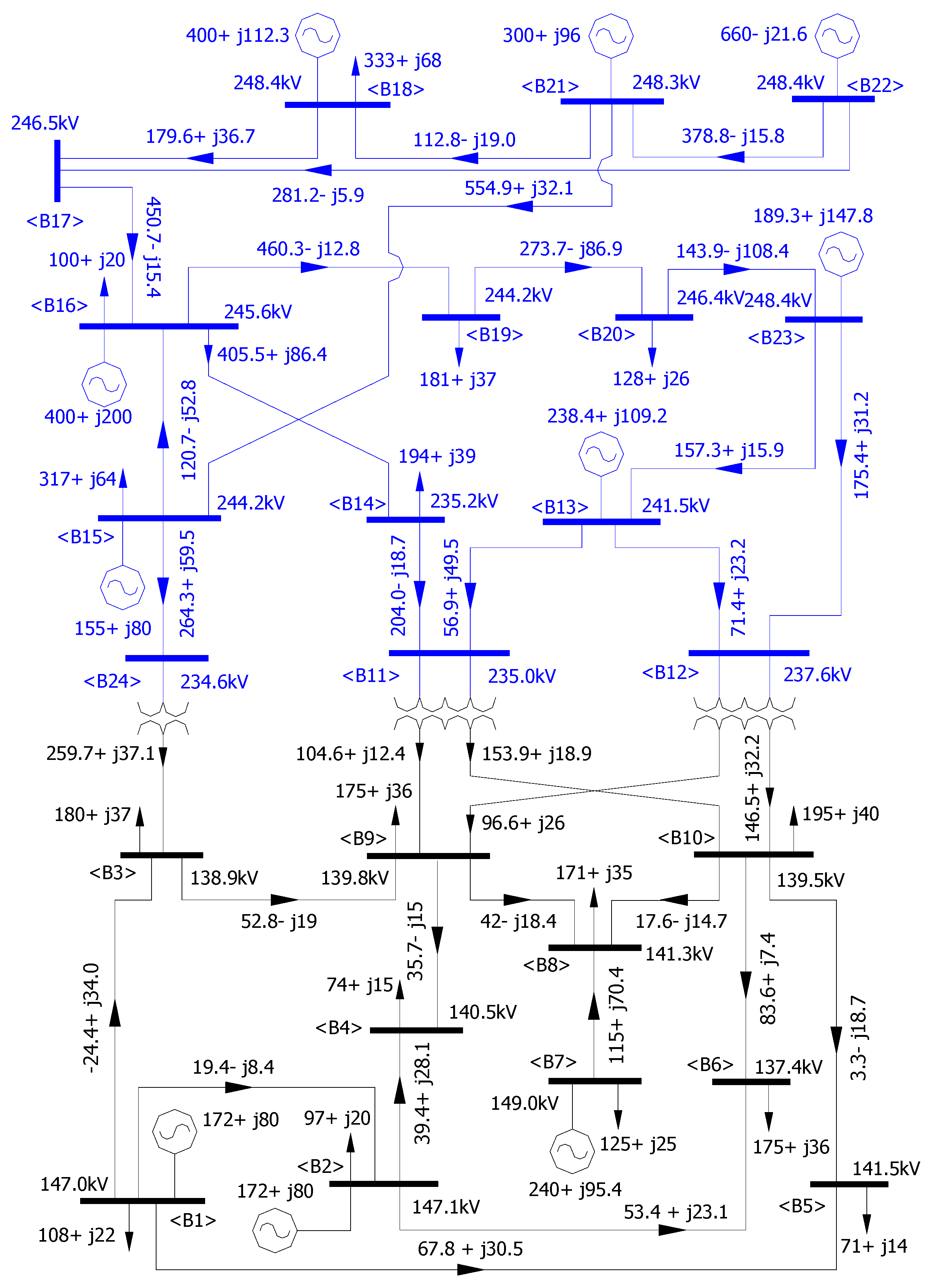
In this section, the methods described in Section 3 are applied to determine the location of STATCOM-POD. The IEEE 24-bus reliability test system is used to investigate the effects of the proposed method for damping the power system oscillations. This network has two voltage levels that are 138 kV and 230 kV, consisting of a total 38 lines and 24 buses, and is model as described in Section 2.2. The data of IEEE 24-bus reliability test system is taken from [46]. All components are established in the PSS/E and MATLAB environments. The result of load flow calculation is shown in Figure 6.
In order to validate the proposed method for the optimal location of STACOM-POD with purpose for damping the power system oscillation, different simulations are carried out on the region of 230 kV voltage level of the IEEE 24-bus reliability test system through the study cases that are discussed as follows:
4.1. Applying the Conventional Method for Optimizing STATCOM-POD Placement and Parameters
The POD controller structure of STATCOM in Figure 3 is considered in this study. In order to seek the best sitting for the STATCOM for damping the oscillatory mode, the STACOM is placed in different buses on the test network except the generator buses. The model residue values associated with critical mode are computed by using the transfer function between the STATCOM active power deviation and its inputs. The parameters for the STACOM are listed in Appendix A.3. The numerical results of the model residues for the transfer function by applying the conventional method introduced in Section 3.2 are shown in Table 1. The test system is supposed that the critical oscillatory mode to the uncontrolled system characterized with the eigenvalue and the relative damping ratio are and , respectively. According to Table 1, the bus number 14 is the most effective placement of the STATCOM since this bus has the largest model residue value. The transfer function for the POD controller of STATCOM can be obtained as:
The value Kp in Equation (46) is calculated by supposing the eigenvalue moves to the desired location from the original location , and can be obtained as:
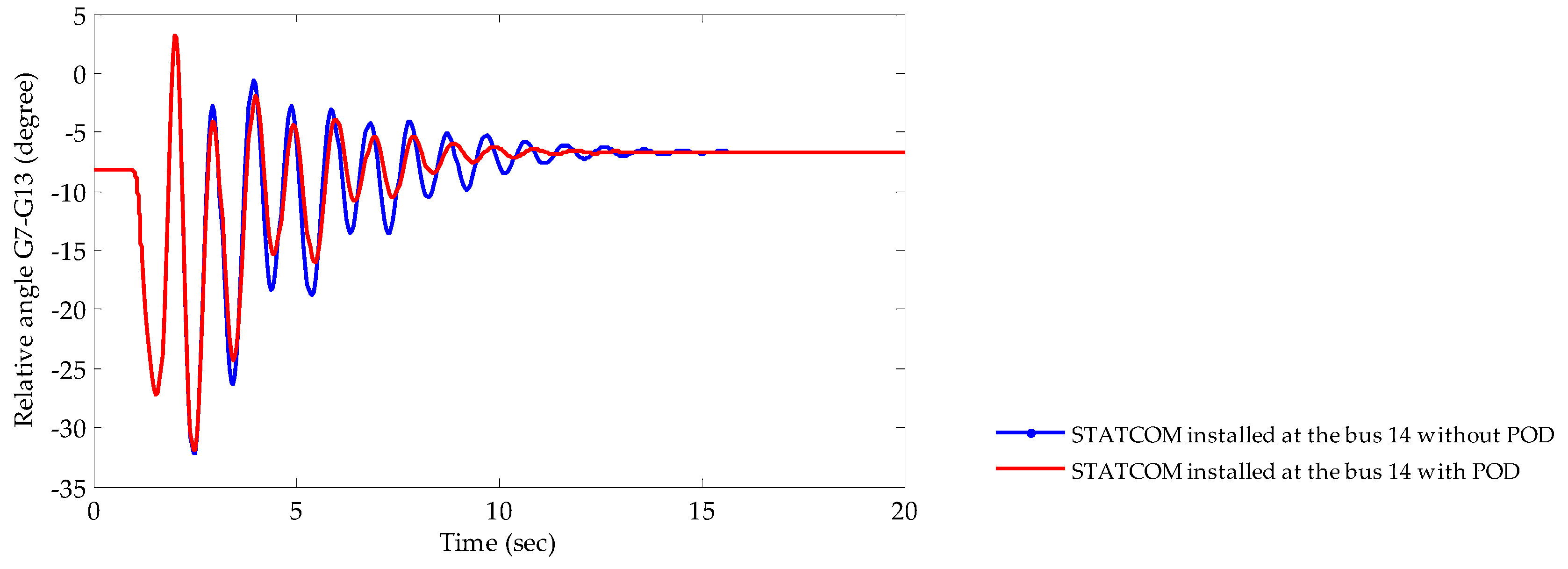
In order to check the efficiency and reliability of the POD controller for STATCOM to the system stability, a three-phase fault is introduced in the line 11–14 close to the bus 14 at 1.0 s and cleared at 1.2 s after by opening the faulted line. A direct comparison between the relative rotor angle swing response of generators 7 and 13 to a three-phase fault with and without POD plotted in Figure 7. It is observed from this figure that the oscillations are damped out after the placement of STATCOM with the POD.
4.2. Applying the Proposed Method for Optimizing STATCOM-POD Placement
The IEEE test network of 24-bus is considered as a larger tested network. This network created the state matrix A. this matrix has dimension [126 × 126] including three states as the transducer, washout, and lead/lag of a STACOM added in the system. The parameters for the STACOM and POD and the input signal for controller are introduced in Section 4.1.
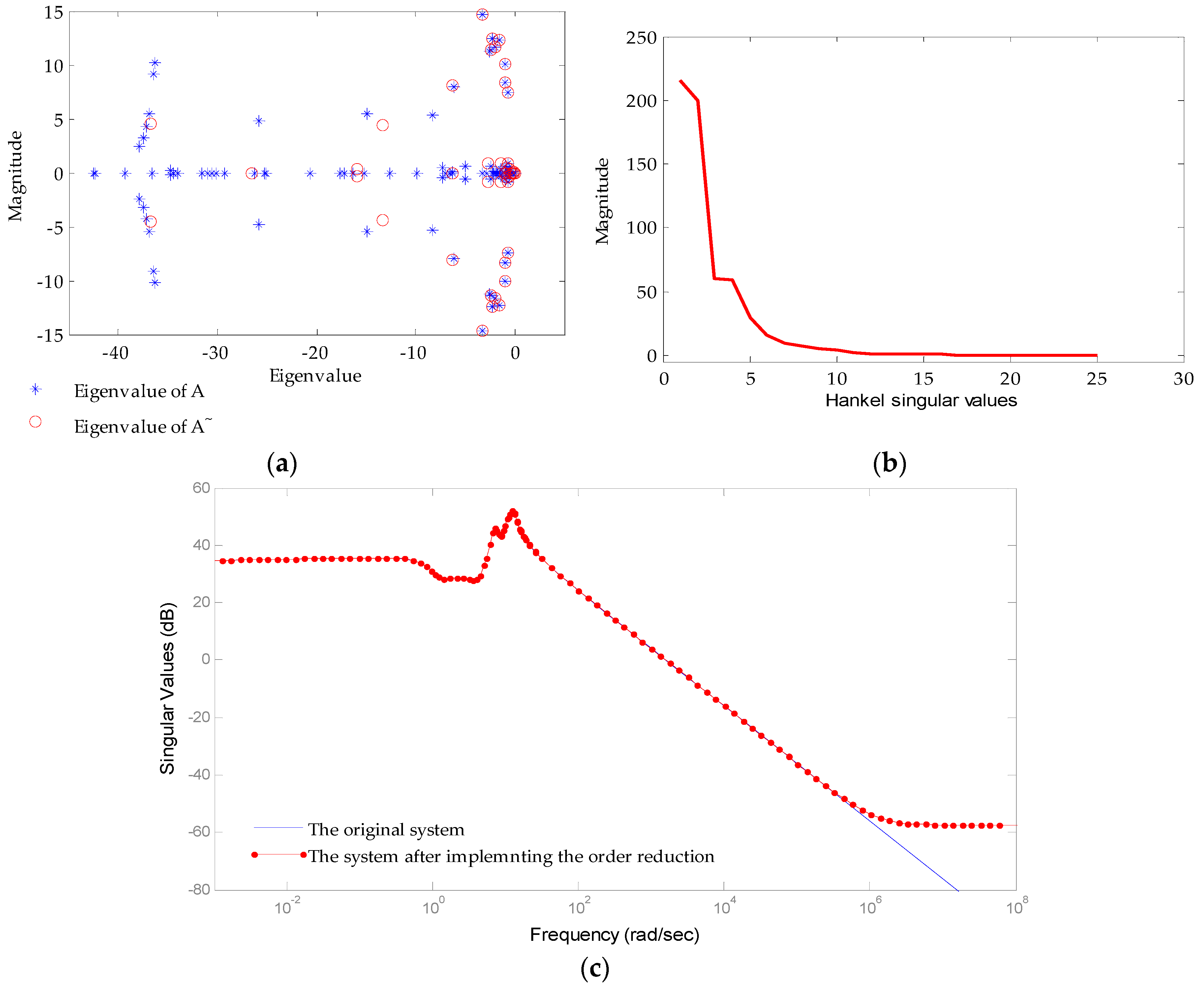
As mentioned in Section 3.1, the order reduction method to eliminate the singular values that are smaller than 10−3 (the threshold value chosen in this study) is implemented. A direct comparison between the eigenvalue of the system state matrix before and after reducing order is given in Figure 8a. According to this figure, the state matrix of the system after reducing order has the dimension [25 × 25]. The new system is only 25 Hankel singular values that are smaller than 10−3 after implementing the order reduction, as shown in Figure 8b. In addition, the result shown in Figure 8c is a comparison of the frequency responses between original and reduced systems. There is no difference between two input–output in the bandwidth from 10−∞ to 106. While the bandwidth from 106 to 10∞, the frequency responses of the reduced system is flat, this means the order of the new system is smaller than that of original system. Therefore, the new system now has 25 state variables, which can fully meet effects of the system to calculate the matrices, and we can conclude that the system before and after reduction is equivalent in terms of robustness.
4.2.1. Determining the Location of the STATCOM-POD Placement
As mentioned in Section 3.3.2, the optimal location of the STATCOM-POD placement is determined based on the objective function in Equation (45) by using the proposed algorithm, and the flowchart shown in Figure 5a, the procedure is given below:
| First. | Start. |
| Step 1. | Place the STATCOM-POD controller at the bus ith (i = 1, 2, 3, …, n)., |
| Step 2. | Run base case load flow, |
| Step 3. | Generate the active power perturbation signal in the transmission line jth. (j = 1, 2, 3, …, m), in which m is large enough. For each contingency of the active power perturbation j. |
| Step 4. | Compute the matrices A, B, C, and D corresponding to the placement ith and the active power perturbation signal jth. |
| Step 5. | Perform the order reduction based on the proposed method in Section 3.1. |
| Step 6. | Estimate the stable condition based on the state matrix to exclude the unstable cases. If the condition is satisfied, Step 6 will be performed; conversely, Step 1 will be iterated. |
| Step 7. | Compute the observability Gramian matrix of the new system corresponding to the active power perturbation signal jth. |
| Step 8. | Iterate the Steps 3 to 7 for computing a set of the active power perturbation (j = 1, 2, 3, …, m). |
| Step 9. | Compute the energy for each placement corresponding to a set of the active power perturbation (j = 1, 2, 3, …, m). |
| Step 10. | Iterate Steps 1 to 7 to calculate all the STATCOM-POD placements (i = 1, 2, 3, …, n). |
| Step 11. | Compare the maximum total energy to evaluate the optimal placement for STATCOM-POD controller based on the objective function in Equation (45). |
| Finally. | End. |
A set of the active power perturbation was selected from single-line outage cases based on the real power flow performance index (PI) introduced in [47] and successfully applied in the literature [2,11,25,48,49]. It can be obtained as:
where nl denotes total number of lines, denotes the exponent, denotes a the non-negative real weighting factor used to reflect the importance for line i, and and are the real power and rated power flows of the line i, respectively. In this simulation, the value of and is selected equal to 1.0 and 2.0, respectively. From that, we have a set of the active power perturbation to consider as the contingency cases listed in Table 2.
The energy values based on Trace of observability Gramian matrix corresponding to the contingency cases as listed in Table 2, which were determined by using the proposed algorithm as shown in Figure 5a, are given in Table 3, where we only listed out several feasible locations (the cases have the high energy values). It can be seen in Table 4 that the bus 17 is the optimal location for STATCOM-POD controller since this location has the highest total energy value compared to other locations; in other words, the energy need to drive the observable state variables is high. Therefore, the bus 17 is the best location to install the controller.
In order to verify the above conclusion, the transient stability analysis of the system is proposed to compare the optimal location with other feasible ones under considering fourth three-phase fault scenarios as shown in Table 4.
- The scenario number 1: A solid three-phase fault occurs at 1 s on line 14–11, close to bus 14, and is cleared after 0.15 s by tripping the faulted line.
- The scenario number 2: A solid three-phase fault occurs at 1 s on line 15–21, close to bus 15, and is cleared after 0.15 s by tripping the faulted line.
- The scenario number 3: A solid three-phase fault occurs at 1 s on line 17–22, close to bus 17, and is cleared after 0.15 s by tripping the faulted line.
- The scenario number 4: A solid three-phase fault occurs at 1 s on line 12–13, close to bus 12, and is cleared after 0.15 s by tripping the faulted line.
The simulations have been performed for each placement of STACOM corresponding to the diminishing total energy value through the following cases:
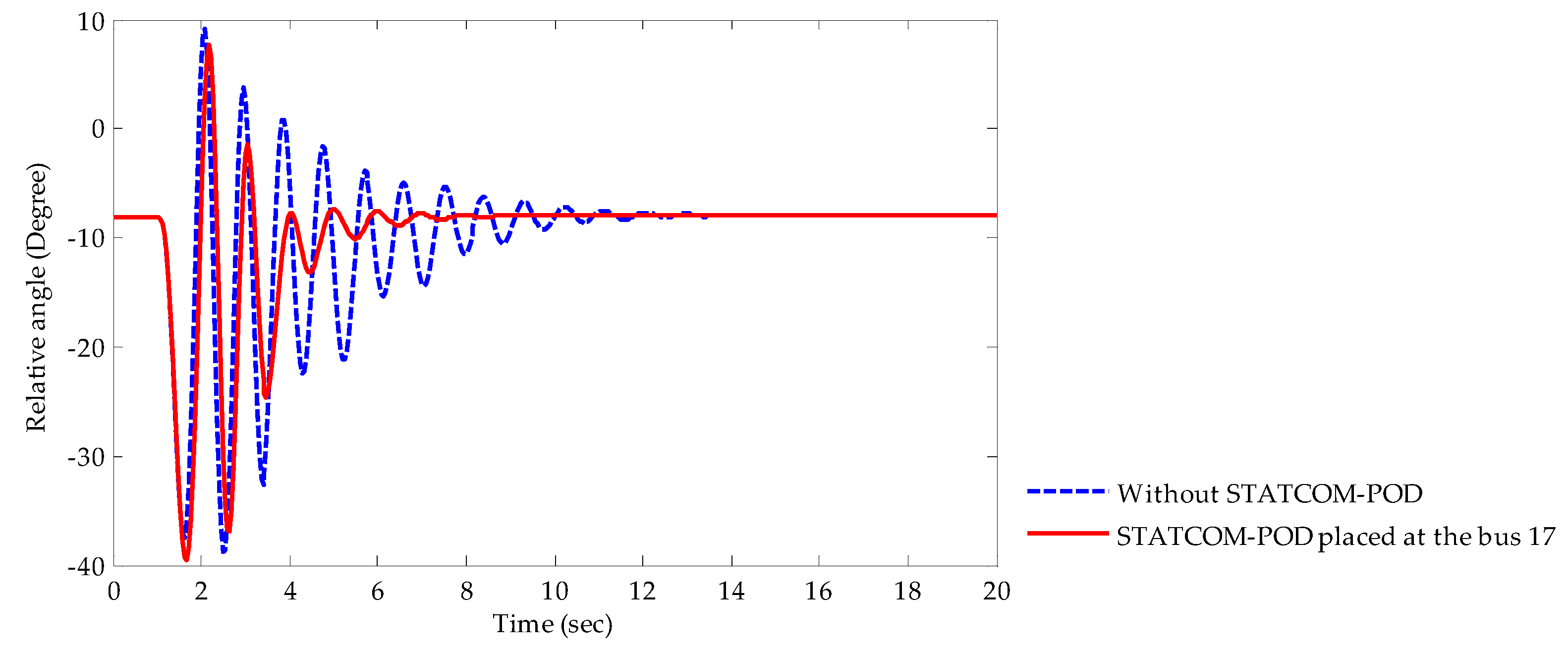
Case 1. The simulation was done on scenario number 1, when the STATCOM_POD is placed at bus 17, the transient respond improves and the oscillations of the relative angle between generators 7 and 13 decreases significantly compared with that is not placed at bus 17, as can be observed from Figure 9.
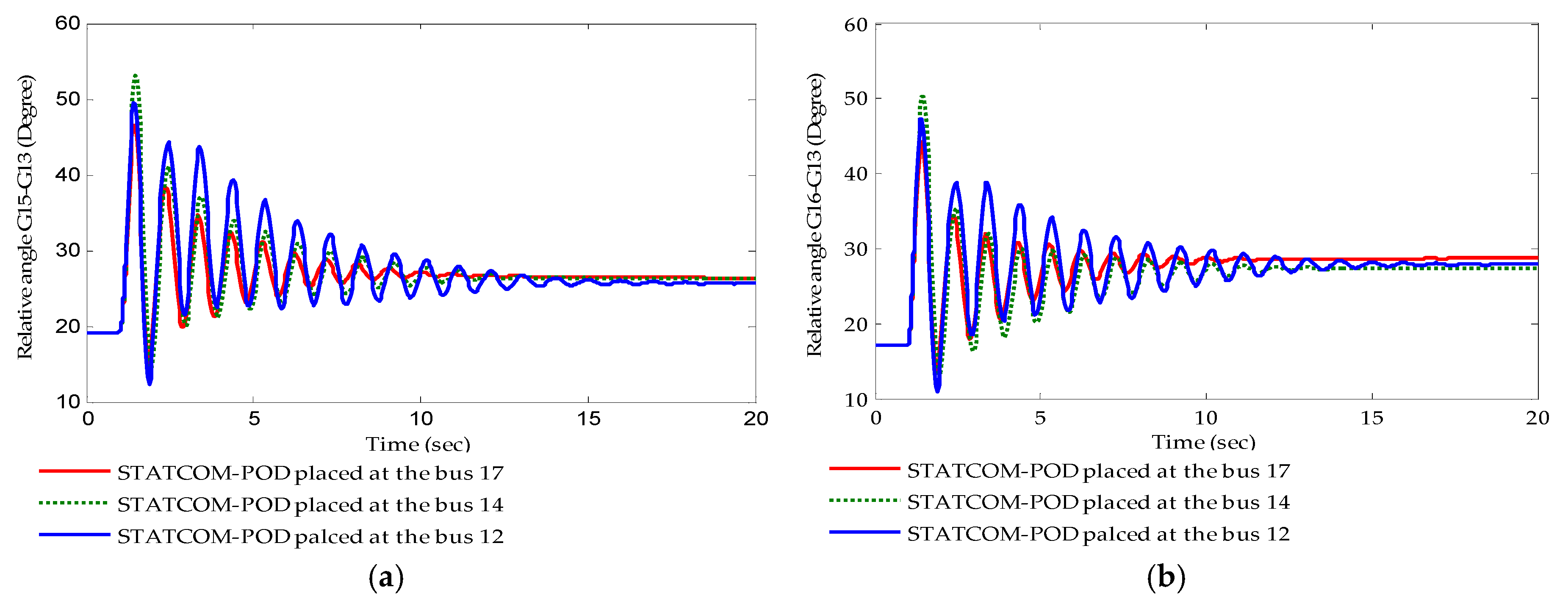
Case 2. In Table 3, it can be seen that buses 17, 14, and 12 have maximum, third, and seventh highest total energy value, respectively. A simulation was done on scenario number 2, when STATCOM-POD is placed at these buses. Figure 10a plots the relative angle between generators 15 and 13; it can be that the transient response improves significantly with STATCOM-POD placed at bus 17. Another simulation was done, and the result is plotted in Figure 10b: the relative angle between generators 16 and 13 is also significantly improved when STATCOM-POD placed at bus 17.
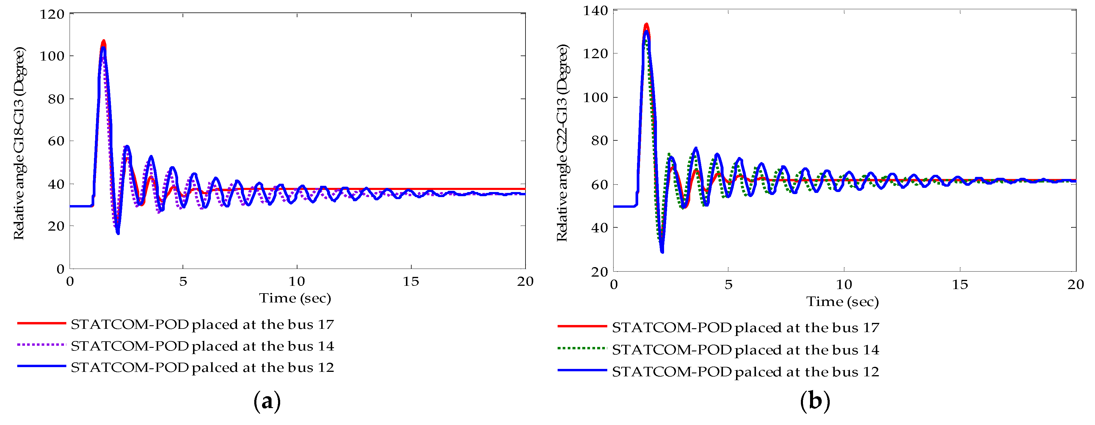
Case 3. Simulation was done on scenario number 3 considering the placement of STATCOM-POD as done in Case 2. Figure 10a,b shows the plot of the relative angle between generators 18 and 22 compared to generator 13. In this case, the STATCOM-POD is placed at bus 17, damping out oscillations of rotor relative angle faster than if placed at buses 14 and 12.
It is also observed in Figure 10 and Figure 11 that the damping of rotor angle oscillations improves with STATCOM-POD placed at bus 14 and this placement provides better damping compared to bus 12.
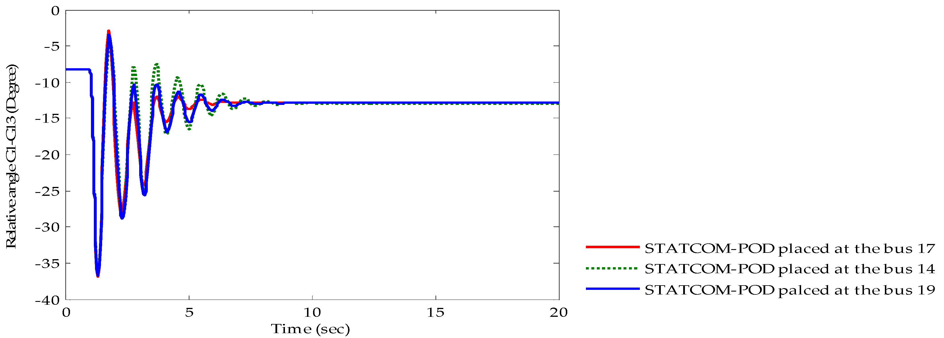
Case 4. In order to make sure “the higher the total energy value, the quicker the damping oscillations”, the simulation in this case was done on scenario number 4, when STATCOM-POD placed at buses 17, 14, and 19. Generator 13 oscillating against generators 1 and 7 was plotted, as shown in Figure 9 and Figure 12. With a fault occurred, the damping ratio is low, so that the damping of oscillations of relative angle between generators 13 and 1 is very slow without STATCOM-POD, as shown in Figure 9.
As can be observed in Figure 12, the transient response improves and oscillations relative angle between generators 1 and 13 decreases significantly with STATCOM-POD is placed at the bus 17 compared with that is placed at buses 14 and 19. In addition, the rotor angle swing response of generators 13 and 1 damped out significantly with STATCOM-POD placed at bus 19 compared with that placed at bus 14. Thus, we could conclude that the location of the STATCOM-POD placement with the purpose for damping the power system oscillations is more reliable on the high observable energy value. Therefore, bus 17 is best location to install the STATCOM-POD controller.
4.2.2. Determining the Location of the Input Signal Placement for STATCOM-POD
After determining the a best location to install STATCOM-POD, the optimal location of feedback signal placement needs to consider for FACTS controllers, it is necessary condition to enhance the system stability.
As mentioned in Section 3.3.1, the optimal location of the signal placement for STATCOM-POD is determined based on the controllable function in Equation (37) by using the proposed algorithm, and the flowchart shown in Figure 5b, the procedure is given below:
| First. | Start. |
| Step 1. | Place the STATCOM-POD controller at the optimal bus i (at bus 17 in this study). |
| Step 2. | Run base case load flow. |
| Step 3. | Generate the active power signal in the transmission line jth (j = 1, 2, 3, …, m). |
| Step 4. | Compute the matrices A, B, C, and D corresponding to the placement i and the active power signal jth. |
| Step 5. | Perform the order reduction based on the proposed method in Section 3.1. |
| Step 6. | Estimate the stable condition based on the state matrix to exclude the unstable cases. If the condition is satisfied, this step will be performed; otherwise, Step 1 will be iterated. |
| Step 7. | Compute the controllability Gramian matrix of the new system corresponding to the active power perturbation signal jth. |
| Step 8. | Iterate Steps 3 to 7 for computing a set of the active power perturbation (j = 1, 2, 3, …, m) corresponding to the i placement. |
| Step 9. | Compute the energy for a set of the active power perturbation (j = 1, 2, 3, …, m). |
| Step 10. | Evaluate the maximum energy in order to determine the optimal location for the input signal placement based on the objective function in Equation (37). |
| Finally. | End. |
The values based on Trace of controllability Gramian matrix, corresponding to a set of input signal, are considered on 17 lines of 230 kV level of IEEE 24-bus network, as given in Table 5. These values were determined by using the proposed algorithm as shown in Figure 5a. It can be seen in Table 5 that the line between buses 23 and 20 is the optimal location of input signal placement for STATCOM-POD controller since this location has the highest value of Trace of controllability Gramian matrix compared to another locations, in other words, the energy need to drive the controllable state variables is small. Therefore, based on the result of the Trace of controllability Gramian matrix, the line between buses 23 and 20 is the best location to be used to install the sensor for receiving and sending the real power flow signal in the transmission line (has been taken as the feedback signal) to the POD of STATCOM.
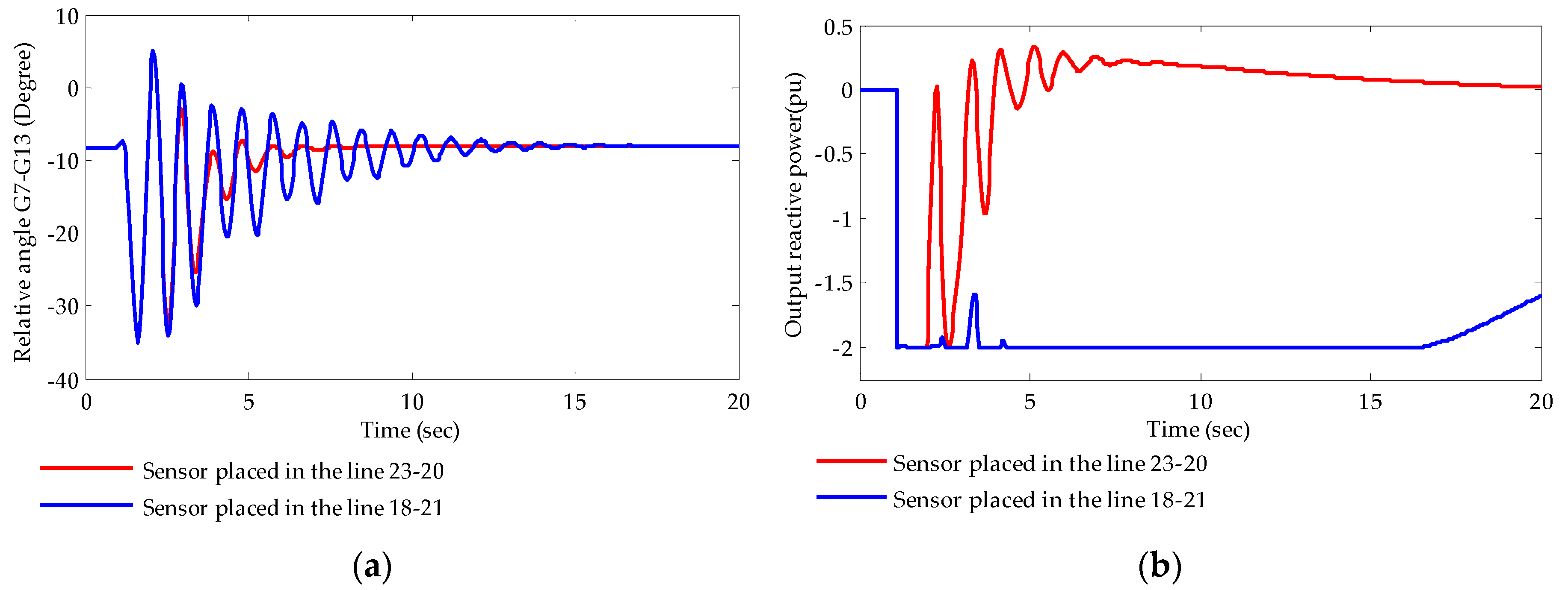
In order to test the system transient stability ability with the received feedback signal from the line having the highest trace value for POD of STATCOM, a three-phase fault was applied on Scenario 3. Comparing between the optimal location (line 23–20) and another location (line 18–21) having minimum energy value based on the output reactive power of controller unit and the rotor angle swing response of between generators 13 and 7 is done. Figure 13 show the plot the transient response of the relative angle between generators 7 and 13 and the output reactive power of STATCOM-POD.
Observing Figure 13a, when the sensor (the device to be used to receive the real power flow from the line and then send it to the POD) is placed in line 23–20, the rotor angle swing response of between generators 13 and 7 is significantly improved compared with that in the line 18–21.
A direct comparison of the output reactive power of controller unit was done to observe the capable of meeting of controller unit. Figure 13b plots this comparison. Evidently, it can be observed from this figure that the sensor is placed in the line 23–20 (POD controller received the active power signal in the line 23–20); the output response of controller unit is quicker than that in the line 18–21. As a result, we could conclude that the location of the input signal placement for STATCOM-POD with the purpose to dampen the power system oscillations is a lot more reliant on the high controllable energy value. Therefore, line 23–20 is best location. This line active power flow has been taken as the feedback signal for supplement controller of STATCOM.
4.3. Comparative Simulation
After applying the proposed method based on the small-signal analysis and retesting one based on the transient analysis, the best location for STATCOM-POD placement is bus 17 and the best location for sensor placement is line 23–20 (POD controller received the active power signal in line 23–20). In addition, according to Table 3, the second-highest total energy value was obtained on the electric power supply system when STATCOM is placed at the bus 19. Vice versa, applying the conventional method as explained and applied in Section 3.1 and Section 4.1, respectively, the best location for STATCOM-POD placement is bus 14.
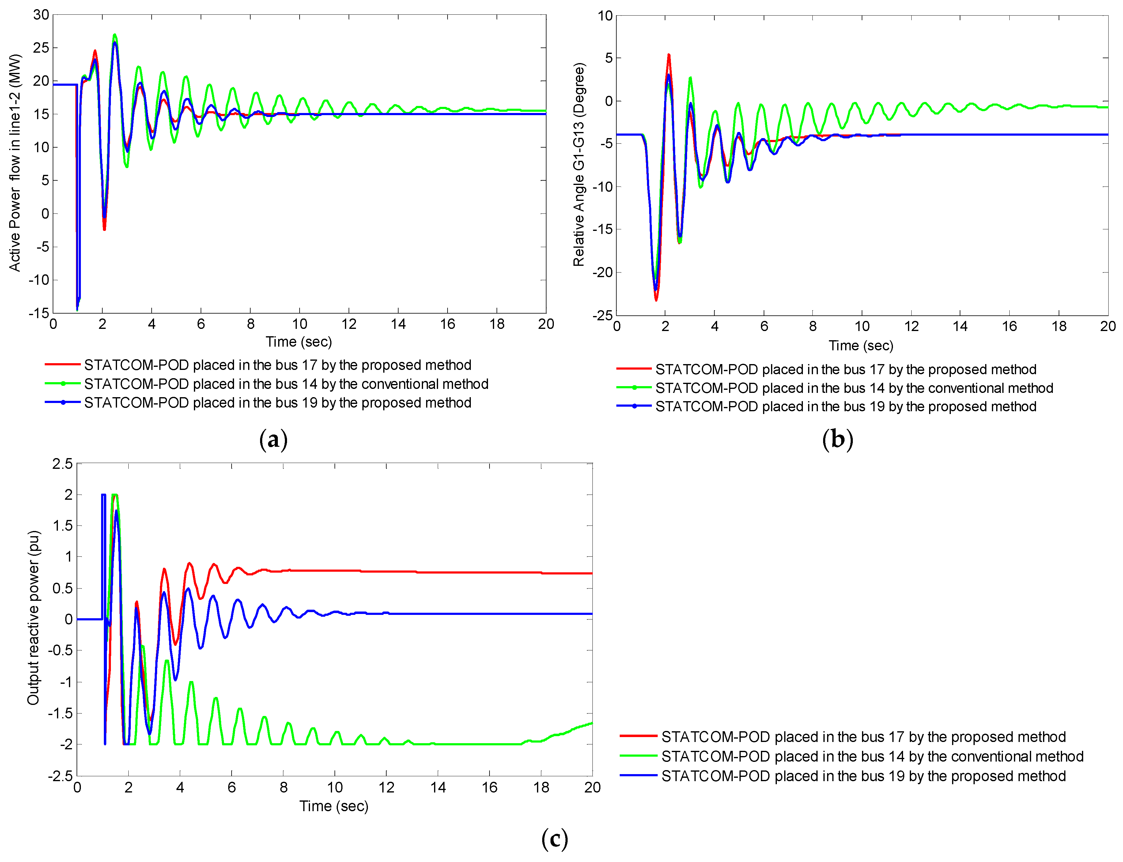
To compare the meeting capable of controller unit for selected location by two methods with main objective to validate further the effectiveness of the proposed method, a direct simulation was done on Scenario number 2, when STATCOM-POD is placed at three locations, buses 14, 17, and 19, based on:
- (i)
- The active power oscillations damping on the transmission line;
- (ii)
- The oscillations damping of the relative angle between generators 7 and 13; and
- (iii)
- The output reactive power response of controller unit.
Figure 14 show the plot of the transient response on Scenario number 2, in which Figure 14a shows the plot of the active power flow in line 1–2. The oscillations are dampened out after STATCOM-POD placement at bus 17 in about 6 s. With STACOM-POD placed at bus 19, the oscillations are dampened out in about 10 s, whereas when STACOM-POD is placed at bus 14, the oscillations are dampened out in about 18 s.
The generator 13 oscillates against generators 1, 2 and 7. With the occurred fault, the critical mode, which damping ratio is very low and is an inter-area mode, gets excited. Because this, the oscillations damping of the relative angle between generators 7 and 13 is slow without STACTCOM-POD, as shown from Figure 9. Figure 14b shows the plot of the oscillations of the relative angle between generators 1 and 13. It can be observed from this figure that the oscillations are damped out in about 6 s, 10 s, and 18 s with STATCOM-POD placed at buses 17, 19, and 14, respectively.
Figure 14c shows the plot of the dynamic response of STATCOM-POD unit corresponding to three locations. Observing this figure, injects to the gird with a reactive power range of −2.0 p.u. to 2.0 p.u. during the period of fault, this output reactive power flow reacted immediately, damped faster, and extremely fast returned to the compensative mode to reach new steady-state after clearing the fault when STATCOM-POD is placed at bus 17. Evidently, it can be observed through above simulation cases, the optimal STATCOM_POD placement and the optimal local input signal placement for POD have been sought by the proposed method provided the effectiveness and robustness of the performance under transient conditions better compared with the conventional method.
5. Conclusions
In this paper, a highly relevant stochastic method for seeking the optimal STATCOM-POD placement and the best location of the sensor (the device using to receive the real power flow from the line and send it to the POD) in the multimachine systems has been proposed with the purpose to dampen the rotor angle oscillations and enhance the transient stability. It is mainly focused on calculation the Gramian matrix of the controllability and observability of the linearized multimachine system based on small-signal analyses. The parameters of the controller obtained from the conventional method. On that basis, the proposed method aims to develop in two steps. Firstly, the optimal STATCOM-POD placement is determined by the algorithm based on the Gramian matrix of the observability on the small-signal stability analyses. Then, test cases of the transient stability are analyzed. The obtained result is no satisfactory since the POD of STACTCOM received the feedback local signal with placement that is not optimal location. In order to overcome this problem, the second step of the proposed method is developed to select the optimal location of the sensor based on the Gramian matrix of the controllability; it was also analyzed based on the small-signal stability and test cases of the transient stability.
The simulation results show that the rotor angle oscillations of generators are significantly dampened when the STATCOM-POD is placed at bus 17 and the sensor is placed in the line between buses number 23 and 20, which have the highest Trace of the Gramian matrix of the controllability and observability. Therefore, it could be concluded that the location of the STATCOM-POD placement with the purpose for damping the power system oscillations is more reliant on the high observable and controllable energy values.
The reduction method based on Krylov-based model reduction solution has also been introduced in this paper for reducing the calculation time of Gramian matrix when dealing with the large-scale power systems.
Acknowledgments
The authors sincerely acknowledge the financial support provided by Duy Tan University, Da Nang, Vietnam, Ton Duc Thang University, Ho Chi Minh, Vietnam, Industrial University of Ho Chi Minh City, Ho Chi Minh, Vietnam, and Quy Nhon University, Binh Dinh, Vietnam for carrying out this work.
Author Contributions
Le Van Dai is the main author of this work, which has been counseled by Doan Duc Tung and Le Cao Quyen.
Conflicts of Interest
The authors declare no conflict of interest.
Appendix A
Appendix A.1. The Arnoldi Algorithm
| Algorithm A1. The Arnoldi Algorithm for a partial realization (s0 = ∞). |
Appendix A.2. The QR Decomposition
Given a matrix Φ, its QR decomposition is a matrix decomposition of the following from:
where R is an upper triangular matrix and Q is an orthogonal matrix, satisfying the following:
The QR decomposition is a function of in Matlab.
Appendix A.3. The Parameters of the STATCOM
| The Parameters of the STATCOM | |||
| Parameter | Value | Parameter | Value |
| T1 | 0.65 s | IStat_Max C | 1 p.u. |
| T2 | 0 s | IStat_Min L | −1 p.u. |
| T3 | 0.2 s | Xt | 0.1 p.u. |
| T4 | 0 s | Limit Max | 1.2 p.u. |
| K | 10 | Limit Min | −1.2 p.u. |
| Droop | 0.02 | SStat | 200 MVAr |
| VMAX | 1.2 p.u. | SBase | 100 MVA |
| VMIN | −1 p.u. | - | - |
References
- AlAli, S.; Haase, T.; Nassar, I.; Weber, H. Impact of increasing wind power generation on the North-South inter-area oscillation mode in the European ENTSO-E system. IFAC Proc. Vol. 2014, 47, 7653–7658. [Google Scholar] [CrossRef]
- Van Dai, L.; Li, X.; Li, P.; Quyen, L.C. An optimal location of static VAr compensator based on Gramian critical energy for damping oscillations in power systems. IEEJ Trans. Electr. Electron. Eng. 2016, 11, 577–585. [Google Scholar] [CrossRef]
- Klein, M.; Rogers, G.J.; Kundur, P. A fundamental study of inter area oscillations in power systems. IEEE Trans. Power Syst. 1991, 6, 914–921. [Google Scholar] [CrossRef]
- Shi, L.; Lee, K.Y.; Wu, F. Robust ESS-Based Stabilizer Design for Damping Inter-Area Oscillations in Multimachine Power Systems. IEEE Trans. Power Syst. 2016, 31, 1395–1406. [Google Scholar] [CrossRef]
- Berizzi, A.; Bovo, C.; Ilea, V. Optimal placement of FACTS to mitigate congestions and inter-area oscillations. In Proceedings of the 2011 IEEE Trondheim in Power Tech, Trondheim, Norway, 19–23 June 2011; pp. 1–8. [Google Scholar]
- Yang, N.; Liu, Q.; McCalley, J.D. TCSC controller design for damping interarea oscillations. IEEE Trans. Power Syst. 1998, 3, 1304–1310. [Google Scholar] [CrossRef]
- Okamoto, H.; Yokoyama, A.; Sekine, Y. Stabilizing control of variable impedance power systems: Applications to variable series capacitor systems. Electr. Eng. Jpn. 1993, 113, 89–100. [Google Scholar] [CrossRef]
- Sui, X.; Tang, Y.; He, H.; Wen, J. Energy-storage-based low-frequency oscillation damping control using particle swarm optimization and heuristic dynamic programming. IEEE Trans. Power Syst. 2014, 29, 2539–2548. [Google Scholar] [CrossRef]
- Du, W.; Wang, H.F.; Cao, J.; Xiao, L.Y. Robustness of an energy storage system-based stabiliser to suppress inter-area oscillations in a multi-machine power system. IET Gener. Transm. Distrib. 2012, 6, 339–351. [Google Scholar] [CrossRef]
- Chen, Z.; Zou, X.; Duan, S.; Wen, J.; Cheng, S. Application of flywheel energy storage to damp power system oscillations. Przegląd Elektrotechniczny 2011, 87, 333–337. [Google Scholar]
- Le, V.; Li, X.; Li, Y.; Cao, Y.; Le, C. Optimal placement of TCSC using controllability Gramian to damp power system oscillations. Int. Trans. Electr. Energy Syst. 2015, 26, 1493–1510. [Google Scholar] [CrossRef]
- Jordehi, A.R. Particle swarm optimisation for dynamic optimisation problems: A review. Neural Comput. Appl. 2014, 25, 1507–1516. [Google Scholar] [CrossRef]
- Rezaee Jordehi, A.; Jasni, J. Parameter selection in particle swarm optimisation: A survey. J. Exp. Theor. Artif. Intell. 2013, 25, 527–542. [Google Scholar] [CrossRef]
- Ghahremani, E.; Kamwa, I. Optimal placement of multiple-type FACTS devices to maximize power system loadability using a generic graphical user interface. IEEE Trans. Power Syst. 2013, 28, 764–778. [Google Scholar] [CrossRef]
- Cai, L.J.; Erlich, I.; Stamtsis, G. Optimal choice and allocation of FACTS devices in deregulated electricity market using genetic algorithms. In Proceedings of the IEEE PES In Power Systems Conference and Exposition, NY, USA, 10–13 October 2004; pp. 201–207. [Google Scholar]
- Saravanan, M.; Slochanal, S.M.R.; Venkatesh, P.; Abraham, J.P.S. Application of particle swarm optimization technique for optimal location of FACTS devices considering cost of installation and system loadability. Electr. Power Syst. Res. 2007, 77, 276–283. [Google Scholar] [CrossRef]
- Abd-Elazim, S.M.; Ali, E.S. Optimal location of STATCOM in multimachine power system for increasing loadability by Cuckoo Search algorithm. Int. J. Electr. Power Energy Syst. 2016, 80, 240–251. [Google Scholar] [CrossRef]
- Khorsandi, A.; Hosseinian, S.H.; Ghazanfari, A. Modified artificial bee colony algorithm based on fuzzy multi-objective technique for optimal power flow problem. Electr. Power Syst. Res. 2013, 95, 206–213. [Google Scholar] [CrossRef]
- Gerbex, S.; Cherkaoui, R.; Germond, A.J. Optimal location of FACTS devices to enhance power system security. In Proceedings of the 2003 IEEE Bologna in Power Tech Conference Proceedings, Bologna, Italy, 23–26 June 2003. [Google Scholar]
- Marouani, I.; Guesmi, T.; Abdallah, H.H.; Ouali, A. Application of a multiobjective evolutionary algorithm for optimal location and parameters of FACTS devices considering the real power loss in transmission lines and voltage deviation buses. In Proceedings of the International Multi-Conference on IEEE in Systems, Signals and Devices, Djerba, Tunisia, 23–26 March 2009. [Google Scholar]
- Lu, Z.; Li, M.S.; Tang, W.J.; Wu, Q.H. Optimal location of FACTS devices by a bacterial swarming algorithm for reactive power planning. In Proceedings of the IEEE Congress on Evolutionary Computation, Suntec, Singapore, 25–28 September 2007; pp. 2344–2349. [Google Scholar]
- Idris, R.M.; Kharuddin, A.; Mustafa, M.W. Optimal choice of FACTS devices for ATC enhancement using bees algorithm. In Proceedings of the Power Engineering Conference, AUPEC, Australasian Universities, Adelaide, Australia, 27–30 September 2009. [Google Scholar]
- Sadikovic, R.; Korba, P.; Andersson, G. Application of FACTS devices for damping of power system oscillations. In Proceedings of the IEEE Russia in Power Tech, Petersburg, Russia, 27–30 June 2005. [Google Scholar]
- Magaji, N.; Mustafa, M.W. Optimal location of FACTS devices for damping oscillations using Residue Factor. In Proceedings of the IEEE 2nd International in Power and Energy Conference, Shinagawa-ku, Tokyo, 1–3 December 2008; pp. 1339–1344. [Google Scholar]
- Kumar, B.K.; Singh, S.N.; Srivastava, S.C. Placement of FACTS controllers using modal controllability indices to damp out power system oscillations. IET Gener. Transm. Distrib. 2007, 1, 209–217. [Google Scholar] [CrossRef]
- Zamora-Cárdenas, A.; Fuerte-Esquivel, C.R. Multi-parameter trajectory sensitivity approach for location of series-connected controllers to enhance power system transient stability. Electr. Power Syst. Res. 2010, 80, 1096–1103. [Google Scholar] [CrossRef]
- Mhaskar, U.P.; Kulkarni, A.M. Power oscillation damping using FACTS devices: Modal controllability, observability in local signals, and location of transfer function zeros. IEEE Trans. Power Syst. 2006, 21, 285–294. [Google Scholar] [CrossRef]
- Eshtehardiha, S.; Kiyoumarsi, A. Optimized performance of STATCOM with PID controller based on genetic algorithm. In Proceedings of the International Conference on Control, Automation and Systems, ICCAS’07, Seoul, Korea, 17–20 October 2007; pp. 1639–1644. [Google Scholar]
- Panda, S.; Patidar, N.P.; Singh, R. Robust coordinated design of excitation and STATCOM-based controller using genetic algorithm. Int. J. Innov. Comput. Appl. 2008, 1, 244–251. [Google Scholar] [CrossRef]
- Safari, A.; Ahmadian, A.; Golkar, M.A.A. Controller design of STATCOM for power system stability improvement using honey bee mating optimization. J. Appl. Res. Technol. 2013, 11, 144–155. [Google Scholar] [CrossRef]
- Abd-Elazim, S.M.; Ali, E.S. Imperialist competitive algorithm for optimal STATCOM design in a multimachine power system. Int. J. Electr. Power Energy Syst. 2016, 76, 136–146. [Google Scholar] [CrossRef]
- Shayeghi, H.; Shayanfar, H.A.; Jalilzadeh, S.; Safari, A. TCSC robust damping controller design based on particle swarmoptimization for a multi-machine power system. Energy Convers. Manag. 2010, 51, 1873–1882. [Google Scholar] [CrossRef]
- Matins, N.; Corsi, S.; Andersson, G.; Gibbard, M.J. Impact of the Interactions among Power System Controllers. Status Report of CIGRE TF 1999, 38, 1–16. [Google Scholar]
- Siemens PTI, PSS/E 30.2 Program Operational Manual; Siemens Power Transmission & Distribution, Inc., Power Technologies International: New York, NY, USA, 2005; Volume 2.
- Zarringhalami, M.; Golkar, M.A. Analysis of power system linearized model with STATCOM based damping stabilizer. In Proceedings of the Third International Conference in IEEE on Electric Utility Deregulation and Restructuring and Power Technologies, Nanjing, China, 6–9 April 2008; pp. 2403–2409. [Google Scholar]
- Sauer, P.W.; Pai, M.A. Power System Dynamics and Stability; Prentice-Hall: Upper Saddle River, NJ, USA, 1998. [Google Scholar]
- Sauer, P.W.; Pai, M.A. Power system steady-state stability and the load-flow Jacobian. IEEE Trans. Power Syst. 1990, 5, 1374–1383. [Google Scholar] [CrossRef]
- Shahnia, F.; Rajakaruna, S.; Ghosh, A. Static Compensators (STATCOMs) in Power Systems; Springer: Berlin/Heidelberg, Germany, 2015. [Google Scholar]
- Laufenberg, M.J.; Pai, M.A.; Padiyar, K.R. Hopf bifurcation control in power systems with static var compensators. Int. J. Electr. Power Energy Syst. 1997, 19, 339–347. [Google Scholar] [CrossRef]
- Mondal, D.; Chakrabarti, A.; Sengupta, A. Power System Small Signal Stability Analysis and Control; Academic Press: London, UK, 2014. [Google Scholar]
- Antoulas, A.C. Approximation of Large-Scale Dynamical Systems; Siam: Philadelphia, PA, USA, 2005. [Google Scholar]
- Saad, Y. Iterative Methods for Sparse Linear Systems; Siam: Philadelphia, PA, USA, 2003. [Google Scholar]
- Pagola, F.L.; Perez-Arriaga, I.J.; Verghese, G.C. On sensitivities, residues and participations: Applications to oscillatory stability analysis and control. IEEE Trans. Power Syst. 1999, 4, 278–285. [Google Scholar] [CrossRef]
- Chen, C.T. Linear System Theory and Design. Oxford University Press, Inc: Oxford, UK, 1995. [Google Scholar]
- Grivet-Talocia, S.; Gustavsen, B. Passive Macromodeling: Theory and Applications; John Wiley & Sons: Hoboken, NJ, USA, 2015. [Google Scholar]
- Subcommittee, P.M. IEEE reliability test system. IEEE Trans. Power Appar. Syst. 1979, 6, 2047–2054. [Google Scholar] [CrossRef]
- Glover, K. All optimal Hankel-norm approximations of linear multivariable systems and their L,∞-error bounds. Int. J. Control 1984, 39, 115–1193. [Google Scholar] [CrossRef]
- Ullah, I.; Gawlik, W.; Palensky, P. Analysis of Power Network for Line Reactance Variation to Improve Total Transmission Capacity. Energies 2016, 9, 936. [Google Scholar] [CrossRef]
- Van Dai, L.; Duc Tung, D.; Le Thang Dong, T.; Cao Quyen, L. Improving Power System Stability with Gramian Matrix-Based Optimal Setting of a Single Series FACTS Device: Feasibility Study in Vietnamese Power System. Complexity 2017, 2017, 3014510. [Google Scholar] [CrossRef]
Figure 1.
The event on 9 February 2006, inter-area oscillations after power plant outage 1.2 GW in Spain.
Figure 1.
The event on 9 February 2006, inter-area oscillations after power plant outage 1.2 GW in Spain.

Figure 2.
Model of STATCOM: (a) Structure; and (b) Voltage–Current characteristic.

Figure 3.
STATCOM dynamic model with the power oscillation damping (POD) controller.

Figure 4.
(a) Power system with STATCOM; (b) Closed-loop system with STATCOM; and (c) Displacement of eigenvalues with the action of the POD controller.
Figure 4.
(a) Power system with STATCOM; (b) Closed-loop system with STATCOM; and (c) Displacement of eigenvalues with the action of the POD controller.

Figure 5.
The flowchart of the proposed method: (a) Determine Location of STATCOM-POD; and (b) Determine location of input signal for POD.
Figure 5.
The flowchart of the proposed method: (a) Determine Location of STATCOM-POD; and (b) Determine location of input signal for POD.

Figure 6.
The result of load flow calculation on the IEEE 24-bus reliability test system.

Figure 7.
The oscillations of the relative angle between generators 7 and 13.

Figure 8.
(a) Eigenvalue before and after implementing order reduction method; (b) Hankel singular values of reduced system; and (c) Frequency response of the original and reduced systems.
Figure 8.
(a) Eigenvalue before and after implementing order reduction method; (b) Hankel singular values of reduced system; and (c) Frequency response of the original and reduced systems.

Figure 9.
The oscillations of the relative angle between generators 1 and 13 for Scenario number 1.

Figure 10.
The transient response for Scenario number 2: (a) The relative angle between generators 15 and 13; (b) The relative angle between generators 16 and 13.
Figure 10.
The transient response for Scenario number 2: (a) The relative angle between generators 15 and 13; (b) The relative angle between generators 16 and 13.

Figure 11.
The transient response for Scenario number 3: (a) The relative angle between generators 18 and 13; (b) The relative angle between generators 22 and 13.
Figure 11.
The transient response for Scenario number 3: (a) The relative angle between generators 18 and 13; (b) The relative angle between generators 22 and 13.

Figure 12.
The oscillations of the relative angle between generators 1 and 13 on Scenario number 4.

Figure 13.
The transient response on Scenario number 3: (a) The relative angle between generators 7 and 13; (b) Output reactive power of STATCOM-POD.
Figure 13.
The transient response on Scenario number 3: (a) The relative angle between generators 7 and 13; (b) Output reactive power of STATCOM-POD.

Figure 14.
The transient response on Scenario number 3: (a) Active power flow in line 1–2; (b) The relative angle between generators 1 and 13; and (c) Output reactive power of STATCOM-POD.
Figure 14.
The transient response on Scenario number 3: (a) Active power flow in line 1–2; (b) The relative angle between generators 1 and 13; and (c) Output reactive power of STATCOM-POD.


Table 1.
Location indices of STATCOM-POD.
| Model Residue Values of the Transfer Function | |
|---|---|
| STATCOM-POD Placed at the Bus | |
| 14 | 0.976 |
| 11 | 0.778 |
| 17 | 0.736 |
| 12 | 0.198 |
| 24 | 0.012 |
| 19 | 0.005 |
| 20 | 0.001 |
Table 2.
Studied contingency cases.
| Case Number | Contingency Case (Active Power Perturbation Signal in the Line between Buses) | Case Number | Contingency Case (Active Power Perturbation Signal in the Line between Buses) |
|---|---|---|---|
| (1) | 11–13 | (10) | 16–17 |
| (2) | 11–14 | (11) | 16–19 |
| (3) | 12–13 | (12) | 17–18 |
| (4) | 12–23 | (13) | 17–22 |
| (5) | 13–23 | (14) | 18–21 |
| (6) | 14–16 | (15) | 19–20 |
| (7) | 15–16 | (16) | 20–23 |
| (8) | 15–21 | (17) | 21–22 |
| (9) | 15–24 | - | - |
Table 3.
Energy values according to several feasible locations of STATCOM-POD controller.
| Case Number | Contingency Case (From Table 2) | Energy Values Based on Trace of Observability Gramian Matrix | ||||||
|---|---|---|---|---|---|---|---|---|
| STATCOM-POD Placed at the Bus | ||||||||
| 11 | 12 | 14 | 17 | 19 | 20 | 24 | ||
| (1) | 11–13 | 82.58 | 62.90 | 89.57 | 294.03 | 153.84 | 112.79 | 157.13 |
| (2) | 11–14 | 494.38 | 277.40 | 427.34 | 680.79 | 503.95 | 382.72 | 373.93 |
| (3) | 12–13 | 170.41 | 97.55 | 136.50 | 229.47 | 149.17 | 114.52 | 144.60 |
| (4) | 12–23 | 251.29 | 223.05 | 221.48 | 356.44 | 289.13 | 311.12 | 210.69 |
| (5) | 13–23 | 234.69 | 177.58 | 221.68 | 404.43 | 261.51 | 268.73 | 225.35 |
| (6) | 14–16 | 618.80 | 218.62 | 691.30 | 619.27 | 434.24 | 360.01 | 333.03 |
| (7) | 15–16 | 299.01 | 235.69 | 387.10 | 642.85 | 452.45 | 307.92 | 366.29 |
| (8) | 15–21 | 469.97 | 387.73 | 498.84 | 818.31 | 579.79 | 419.27 | 609.25 |
| (9) | 15–24 | 308.28 | 205.19 | 272.09 | 447.37 | 361.44 | 298.43 | 397.58 |
| (10) | 16–17 | 491.35 | 305.15 | 573.04 | 852.46 | 656.52 | 463.65 | 490.95 |
| (11) | 16–19 | 428.88 | 321.11 | 548.22 | 1020.29 | 855.97 | 600.79 | 562.90 |
| (12) | 17–18 | 291.69 | 230.46 | 337.48 | 666.07 | 441.14 | 310.05 | 338.04 |
| (13) | 17–22 | 271.33 | 292.01 | 278.07 | 454.16 | 295.42 | 209.23 | 237.74 |
| (14) | 18–21 | 104.00 | 94.42 | 109.06 | 255.49 | 140.14 | 106.10 | 169.33 |
| (15) | 19–20 | 359.08 | 282.60 | 545.56 | 1071.40 | 760.24 | 523.01 | 611.26 |
| (16) | 20–23 | 300.10 | 208.97 | 529.71 | 1108.86 | 776.81 | 491.31 | 646.05 |
| (17) | 21–22 | 356.14 | 295.10 | 363.93 | 557.35 | 382.87 | 285.16 | 366.80 |
| Total | 5531.97 | 3915.53 | 6230.94 | 10479.04 | 7494.62 | 5564.79 | 6240.92 | |
Table 4.
Scenarios on three-phase fault for test of transient stability.
| Scenario Number | Fault Is nearly Bus | Start Time | Closed Time | Line Outage between Buses |
|---|---|---|---|---|
| (1) | 14 | 1 | 1.2 | 14–11 |
| (2) | 15 | 1 | 1.1 | 15–21 |
| (3) | 17 | 1 | 1.1 | 17–22 |
| (4) | 12 | 1 | 1.2 | 12–13 |
Table 5.
Energy values according to a set of input signal location with STATCOM-POD placed at bus 17.
Table 5.
Energy values according to a set of input signal location with STATCOM-POD placed at bus 17.
| Case Number | Active Power Signal in the Line between Buses | Trace Value of Controllability Gramian Matrix | Index |
|---|---|---|---|
| (1) | 14–16 | 622.40 | 0.49 |
| (2) | 19–16 | 1030.32 | 0.82 |
| (3) | 18–17 | 617.00 | 0.49 |
| (4) | 17–16 | 984.65 | 0.78 |
| (5) | 11–14 | 645.46 | 0.51 |
| (6) | 15–21 | 794.08 | 0.63 |
| (7) | 15–16 | 607.81 | 0.48 |
| (8) | 11–13 | 486.66 | 0.39 |
| (9) | 12–13 | 406.34 | 0.32 |
| (10) | 13–23 | 395.03 | 0.31 |
| (11) | 18–21 | 266.74 | 0.21 |
| (12) | 12–23 | 395.03 | 0.31 |
| (13) | 17–22 | 342.55 | 0.27 |
| (14) | 21–22 | 595.58 | 0.47 |
| (15) | 23–20 | 1261.78 | 1.00 |
| (16) | 15–24 | 566.31 | 0.45 |
| (17) | 19–20 | 1058.28 | 0.84 |
© 2017 by the authors. Licensee MDPI, Basel, Switzerland. This article is an open access article distributed under the terms and conditions of the Creative Commons Attribution (CC BY) license (http://creativecommons.org/licenses/by/4.0/).
Share and Cite
MDPI and ACS Style
Dai, L.V.; Tung, D.D.; Quyen, L.C. A Highly Relevant Method for Incorporation of Shunt Connected FACTS Device into Multi-Machine Power System to Dampen Electromechanical Oscillations. Energies 2017, 10, 482. https://doi.org/10.3390/en10040482
AMA Style
Dai LV, Tung DD, Quyen LC. A Highly Relevant Method for Incorporation of Shunt Connected FACTS Device into Multi-Machine Power System to Dampen Electromechanical Oscillations. Energies. 2017; 10(4):482. https://doi.org/10.3390/en10040482
Chicago/Turabian StyleDai, Le Van, Doan Duc Tung, and Le Cao Quyen. 2017. "A Highly Relevant Method for Incorporation of Shunt Connected FACTS Device into Multi-Machine Power System to Dampen Electromechanical Oscillations" Energies 10, no. 4: 482. https://doi.org/10.3390/en10040482
Note that from the first issue of 2016, this journal uses article numbers instead of page numbers. See further details here.