Energy Trading and Pricing in Microgrids with Uncertain Energy Supply: A Three-Stage Hierarchical Game Approach

Abstract

This paper studies an energy trading and pricing problem for microgrids with uncertain energy supply. The energy provider with the renewable energy (RE) generation (wind power) determines the energy purchase from the electricity markets and the pricing strategy for consumers to maximize its profit, and then the consumers determine their energy demands to maximize their payoffs. The hierarchical game is established between the energy provider and the consumers. The energy provider is the leader and the consumers are the followers in the hierarchical game. We consider two types of consumers according to their response to the price, i.e., the price-taking consumers and the price-anticipating consumers. We derive the equilibrium point of the hierarchical game through the backward induction method. Comparing the two types of consumers, we study the influence of the types of consumers on the equilibrium point. In particular, the uncertainty of the energy supply from the energy provider is considered. Simulation results show that the energy provider can obtain more profit using the proposed decision-making scheme.

1. Introduction

In the microgrid, energy trading is an important segment [1,2]. The energy provider determines the energy purchase to meet the consumer demands. Meanwhile, in order to increase its profit, the energy provider faces a problem of pricing decision. With the development of renewable energy (RE), it is reasonable for the energy provider to use the renewable energy as supply [3,4]. Due to the introduction of the renewable energy, the energy provider has to predict the generating capacity of the renewable energy system, and then decides how much energy it needs to purchase from the electricity markets. The energy provider’s prediction can have a deviation from the actual generation, which leads to the uncertainty (UC) of the energy supply [5,6,7].

There are some works in literature related to the interactions among the consumers. A non-cooperative game (NCG) was formulated among the consumers in [8,9,10,11,12,13,14]. In [9], the price-taking consumers and the price-anticipating consumers were considered. The price-taking consumers assume that their energy consumption cannot affect the electricity price, whereas the price-anticipating consumers believe that their energy consumption can change the electricity price. Recently, the Stackelberg game (SG) is formulated between the energy provider and the consumers in [15,16,17,18,19,20]. In addition, the authors in [20,21] took into account a two-stage Stackelberg game between the power station and the consumers. In order to reduce the cost of the energy purchased from the electricity markets, the renewable energy was taken into account in [22]. Most of these works mainly focus on the price-taking consumers, and they seldom take into account the renewable energy generation, thereby the uncertainty of the energy supply is not involved. The differences of the proposed work with the above literature are shown in

Table 1. Differences of the proposed work with the literature.

Indexes	RE	UC	NCG	SG
[3,4]	√	×	×	×
[5,6,7]	×	√	×	×
[8,9,10,11,12,13,14]	×	×	√	×
[15,16,17,18,19,20,21]	×	×	×	√
This work	√	√	√	√

.

In this paper, we consider the uncertainty of the energy supply caused by the wind power generation. Furthermore, we both consider the price-taking consumers and the price-anticipating consumers. We model the interactions between the energy provider and the consumers as a three-stage hierarchical game. The energy provider, which is the hierarchical game’s leader, determines the price and the energy purchase to maximize its profit. Finally, we obtain the equilibrium of the hierarchical game through the backward induction method [23,24].

The rest of the paper is organized as follows. Section 2 introduces the problem formulation. Section 3 shows the backward induction method of the three-stage hierarchical game for the energy provider and the price-taking consumers. In Section 4, the backward induction method of the three-stage game for the energy provider and the price-anticipating consumers is described. Section 5 gives the simulation and comparison results. Finally, the conclusions are summarized in Section 6.

2. Problem Formulation

We consider the energy trading and pricing problem in the microgrid consisting of one energy provider and a set $\mathbb{N}=\{1,...,N\}$ of consumers. The energy provider and the consumers are integrated into a microgrid with renewable energy generation. The energy provider purchases energy from the electricity markets when the renewable energy supply is not enough. In that case, the energy supply includes the energy generated from the renewable energy source and the energy purchased from the electricity markets. In the microgrid, the system structure of the energy trading is given in Figure 1. Because of the uncertainty of the energy generated from renewable energy sources, the energy purchased from the electricity markets is uncertain. According to the interaction between the energy provider and the consumers, we establish a hierarchical game as below.

• Leader: the energy provider determines the energy purchase and the pricing strategy to maximize its profit.
• Followers: the consumers determine the energy demands to maximize their payoffs.

According to the types of the consumers, we consider two scenarios in this paper. In scenario A, there is no competition among the price-taking consumers, i.e., the consumers’ energy consumption cannot affect the price announced by the energy provider. In scenario B, the interactions among the price-anticipating consumers are formulated into a non-cooperative game, i.e., the consumers’ energy consumption can change the price announced by the energy provider [9].

3. Wind Power Generation Model

There exists a large body of literature on wind power forecasting, and the day-ahead wind forecast based on numerical weather prediction (NWP) models can enable relatively accurate wind forecasts [25,26]. Because the operating time moves closer to the near term, the computation complexity often renders NWP models intractable at a high spatial resolution [26]. An adaptive wavelet neural network was proposed for mapping the NWP’s wind speed and wind direction forecasts to wind power forecasts in [27]. The authors in [28] proposed a novel statistical wind power forecast framework, which leverages the spatio-temporal correlation in wind speed and direction data among geographically dispersed wind farms. In [29], the author developed a feed-forward neural network approach for wind power generation forecasting to improve the wind forecasting accuracy. However, the wind power forecast is relatively complex, and the forecast errors cannot be avoided. Generally, the wind speed can be approximated as the Gamma distribution [30], inverse Gaussian [31], log-normal [32], and Weibull [33,34,35,36]. Alternatively, copula theory has recently been applied to wind speed and wind power as a way of modeling nonlinear dependence structures [37]. According to the wind speed, we establish the wind power generation model adopting the mixed copula function in this paper. Firstly, we introduce the copula theory.

The copula theory was proposed by Sklar in 1959 [38]. Supposing that $F(x_1,x_2,\cdots ,x_N)$ is a joint distribution function whose marginal distributions are $F_1(x_1),F_2(x_2),\cdots ,F_N(x_N)$, then there is a copula function C satisfies [39]:

$$\begin{array}{c}\hfill F(x_1,x_2,\cdots ,x_N)=C(F_1(x_1),F_2(x_2),\cdots ,F_N(x_N)).\end{array}$$

(1)

Defining that $F_1^{-1}(u_1),F_2^{-1}(u_2),\cdots ,F_N^{-1}(u_N)$ are the pseudo inverse functions of $F_1(x_1),F_2(x_2),\cdots ,F_N(x_N)$, respectively. Therefore, the copula function C can be obtained as the following:

$$\begin{array}{c}\hfill C(u_1,u_2,\cdots ,u_N)=F(F_1^{-1}(u_1),F_2^{-1}(u_2),\cdots ,F_N^{-1}(u_N)),\end{array}$$

(2)

where the marginal distributions of $C(u_1,u_2,\cdots ,u_N)$ follow uniform distribution in $[0,1]$ [40].

When $N=2$, the copula function C is a binary function. $H(x_1,x_2)$ is a joint distribution function whose marginal distributions are $F(x_1)$ and $W(x_2)$, and $F^{-1}(u)$ and $W^{-1}(v)$ are the pseudo inverse function of $F(x_1)$ and $W(x_2)$, respectively. Therefore, the copula function C is expressed as the following:

$$\begin{array}{c}\hfill C(u,v)=H(F^{-1}(u),W^{-1}(v)).\end{array}$$

(3)

The mixed copula function was further proposed in [41,42]:

$$\begin{array}{c}\hfill C_M(u,v)={\lambda }_1{C}_1(u,v,{\gamma }_1)+{\lambda }_2{C}_2(u,v,{\gamma }_2)+{\lambda }_3{C}_3(u,v,{\gamma }_3),\end{array}$$

(4)

where $C_M(u,v)$ is the mixed copula function that is composed of $C_1(u,v,{\gamma }_1)$, $C_2(u,v,{\gamma }_2)$, and $C_3(u,v,{\gamma }_3)$. ${\lambda }_1$, ${\lambda }_2$, and ${\lambda }_3$ are weight coefficients of $C_1(u,v,{\gamma }_1)$, $C_2(u,v,{\gamma }_2)$, and $C_3(u,v,{\gamma }_3)$, respectively, and satisfy ${\lambda }_1+{\lambda }_2+{\lambda }_3=1$. ${\gamma }_1$, ${\gamma }_2$, and ${\gamma }_3$ are correlation coefficients and can measure the correlation degree of variables.

The results of [41] showed that the relevant structures of the mixed copula function are more flexible than a single copula function. The wind power generation model is established by the mixed copula function (see details in [38]).

4. Scenario A: The Three-Stage Game for Price-Taking Consumers

In this section, we prove the existence and uniqueness of the hierarchical equilibrium by using the backward induction method. First, we analyze the consumers’ demands given the energy provider’s pricing strategy and energy purchase. Then, we study the energy provider’s pricing strategy given the consumers’ energy demands and the energy purchase. Finally, we analyze the energy purchased from the electricity markets in the case of uncertain renewable generation, and then obtain the maximum profit of the energy provider.

4.1. Consumer’s Energy Demands in Stage III

In Stage I, the energy provider needs to determine the energy purchased from the electricity markets. In Stage II, the energy provider announces the price to the consumers. In Stage III, the consumers determine their energy demands given the unit price p announced by the energy provider in Stage II. The payoff of consumer i is defined as the difference between the satisfaction level and the payment for energy purchase, i.e.,

$$\begin{array}{c}\hfill u_i(p,c_i)=-h{(c_i-c_i^{{}^{\prime }})}^2-p{c}_i,\end{array}$$

(5)

where h is the consumers’ cost coefficient, $c_i$ is the actual energy demand of the consumer i, and $c_i^{{}^{\prime }}$ is the energy demand of the consumer i to maintain normal operation of appliances. The consumers determine their demands to maximize their payoffs. p is a fixed price announced by the energy provider.

The first derivative of $u_i(p,c_i)$ with respect to $c_i$ is:

$$\begin{array}{c}\hfill \frac{\partial u_i(p,c_i)}{\partial c_i}=-2h(c_i-c_i^{{}^{\prime }})-p.\end{array}$$

(6)

Letting $\partial u_i(p,c_i)/\partial c_i=0$, we obtain:

$$\begin{array}{c}\hfill -2h(c_i-c_i^{{}^{\prime }})-p=0,\forall i\in N.\end{array}$$

(7)

From Equation (7), we can obtain the energy demands of the consumer i:

$$\begin{array}{c}\hfill c_i(p)=c_i^{{}^{\prime }}-\frac{p}{2h}.\end{array}$$

(8)

Adding Equation (8) from 1 to N, we obtain the total energy consumption of all consumers:

$$\begin{array}{c}\hfill \sum _{i\in N}{c}_i^{*}(p)=\sum _{i\in N}{c}_i^{{}^{\prime }}-\frac{pN}{2h}.\end{array}$$

(9)

We assume that $Q={\sum }_{i\in N}{c}_i^{{}^{\prime }}$ for convenience. When all consumers’ total demands are ${\sum }_{i\in N}{c}_i^{*}(p)$, the payoffs of the consumers are at a maximum. Next, we consider how the energy provider makes the purchase strategy and pricing strategy in Stages I and II based on the total energy demands, respectively. In particular, we show that the energy provider can determine a price in Stage II such that the total energy demands (as a function of price) cannot exceed the total energy supply.

4.2. Optimal Pricing Strategy in Stage II

In Stage II, the energy provider determines the pricing strategy according to the consumers’ energy demands, given the energy purchase in Stage I. The profit of the energy provider is denoted by:

$$\begin{array}{c}\hfill W(p_s,\beta )=\min (p\sum _{i\in N}{c}_i^{*}(p),p(\beta +{\beta }_0)p_s)-\mu {\beta }_0{p}_s-p_w\beta p_s,\end{array}$$

(10)

which is the difference between the revenue and the total cost. We assume that $p_s$ is the summation of the energy generated from the renewable energy source and the energy purchased from the electricity markets. ${\beta }_0{p}_s$ indicates the energy purchase, $\beta$ is the uncertainty factor of the renewable energy source, $\beta p_s$ is the wind power generation, and $\mu$ is the energy provider’s cost coefficient. In this paper, the energy provider’s cost comes from the energy purchase and the wind power generation. $p_w$ is the cost coefficient and $p_w\beta p_s$ is the wind power generating cost. Equation (10) denotes the fact that the revenue of the energy provider is determined by the consumers’ demands subject to its available supply. In Stage II, the objective is to find the optimal price p that maximizes the energy provider’s profit, i.e.,

$$\begin{array}{c}\hfill W_{II}(p_s,\beta )=\underset{p\ge 0}{max}W(p_s,\beta ),\end{array}$$

(11)

where $W_{II}(p_s,\beta )$ denotes the maximum profit of the energy provider in Stage II. Since the energy supply $p_s$ from the energy provider is given in this stage, the total cost $\mu {\beta }_0{p}_s$ is already fixed. Therefore, the maximum revenue can be achieved by optimizing the price:

$$\begin{array}{c}\hfill \underset{p\ge 0}{max}min(p\sum _{i\in N}{c}_i^{*}(p),p(\beta +{\beta }_0)p_s).\end{array}$$

(12)

Let us define the consumers’ energy demands $D(p)=p{\sum }_{i\in N}{c}_i^{*}$ and the energy supply $S(p)=p\beta p_s$. Then, we have:

$$\begin{array}{ccc}\hfill D(p)& =& -\frac{N{p}^2}{2h}+Qp,\hfill \end{array}$$

(13)

$$\begin{array}{ccc}\hfill S(p)& =& p(\beta +{\beta }_0)p_s.\hfill \end{array}$$

(14)

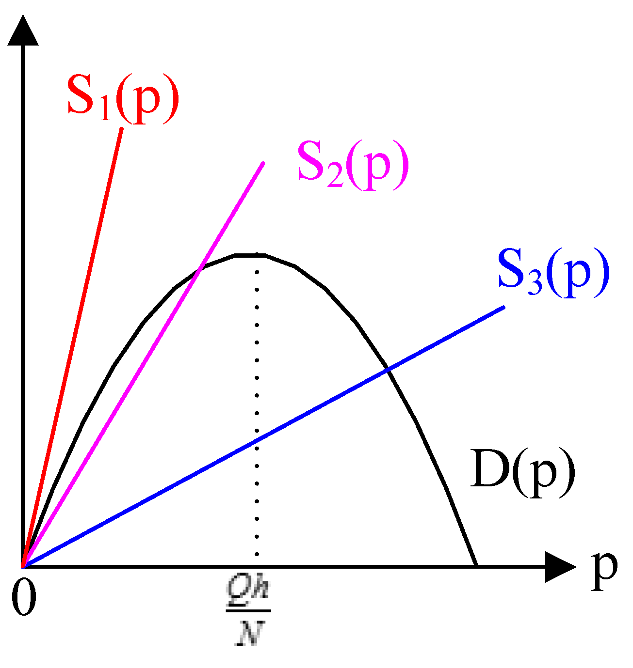
From the above equations, we observe that $D(p)$ is a quadratic function, and $S(p)$ is a linear function. Thus, we can obtain the maximum point of $D(p)$ at $p_d=Qh/N$. The relationships between $S(p)$ and $D(p)$ are described in Figure 2.

• $S_1(p)$ (excessive supply): $S_1(p)$ doesn’t intersect with $D(p)$, $p^{*}=p_d$;
• $S_2(p)$ (excessive supply): $S_2(p)$ has one intersection with $D(p)$, where $D(p)$ has a non-negative slope, $p^{*}=p_d$;
• $S_3(p)$ (conservative supply): $S_3(p)$ has one intersection with $D(p)$, where $D(p)$ has a negative slope, $p^{*}=p_h$, where $p_h$ is the intersection point of $D(p)$ and $S(p)$ and $p^{*}$ is the optimal price announced by the energy provider.

Letting $D(p)=S(p)$, we obtain a quadratic function with respect to p and make it equal to zero:

$$\begin{array}{c}\hfill -\frac{N{p}^2}{2h}+(Q-(\beta +{\beta }_0)p_s)p=0.\end{array}$$

(15)

Solving the above Equation (15), we obtain the intersection point of $D(p)$ and $S(p)$:

$$\begin{array}{c}\hfill p_h=\frac{2h(Q-(\beta +{\beta }_0)p_s)}{N}.\end{array}$$

(16)

In the excessive supply regime, the maximum profit of the energy provider is at $p=p_d$:

$$\begin{array}{c}\hfill W_{II}^{ES}=\frac{h{Q}^2}{2N}-\mu {\beta }_0{p}_s-p_w\beta p_s.\end{array}$$

(17)

In the conservative supply regime, the maximum profit of the energy provider is at $p=p_h$:

$$\begin{array}{c}\hfill W_{II}^{CS}=\frac{2h(Q-(\beta +{\beta }_0)p_s)}{N}(\beta +{\beta }_0)p_s-\mu {\beta }_0{p}_s-p_w\beta p_s.\end{array}$$

(18)

The optimal pricing decision and the corresponding optimal profit at Stage II are given in

Table 2. Optimal pricing decision and profit in Stage II in scenario A.

Total Energy Obtained	Optimal Price	Optimal Profit
in Stages I and II	${\mathit{p}}^{*}({\mathit{p}}_{\mathbf{s}},\mathit{\beta })$	${\mathit{W}}_{\mathbf{II}}({\mathit{p}}_{\mathbf{s}},\mathit{\beta })$
Excessive Supply Regime: $p_s\ge \frac{Q}{2}$	$p^{ES}=p_d$	$W_{II}^{ES}(p_s,\beta )$ in Equation (17)
Conservative Supply Regime: $p_s<\frac{Q}{2}$	$p^{CS}=p_h$	$W_{II}^{CS}(p_s,\beta )$ in Equation (18)

4.3. Energy Supply Strategy in Stage I

In Stage I, the energy provider determines the energy purchase to maximize its profit by taking into account the uncertainty factor of the energy supply $\beta$ [15]. The profit of the energy provider in the Stage I is given as follows:

$$\begin{array}{c}\hfill W_I=\underset{p_s\ge 0}{max}{W}_{II}(p_s,\beta ),\end{array}$$

(19)

where $W_{II}(p_s,\beta )$ is the energy provider’s profit functions with respect to $p_s$ and the uncertain factor $\beta$ obtained in Stage II.

We assume that the wind power generation $P=\beta p_s$, and the minimum power and maximum power of the wind power generation are $P_{\min }$ and $P_{\max }$, respectively. The probability density function of the wind power $f_{WP}(P)$ can be obtained in [38]. From Figure 2, we can obtain that the maximum consumers’ demands ${\sum }_{i\in N}{c}_i^{*}(p)$ is $Q/2$ when the price p is $Qh/N$. Thus, we consider the following two intervals:

(1)

Interval I: $p_s\in [0,\frac{Q}{2}]$. In this interval, the energy provider’s profit function is:

$$\begin{array}{cc}\hfill W_{II}^1(p_s)& =E_{P\in [P_{\min },P_{\max }]}\left[W_{II}^{CS}(P)\right]\hfill \\ & ={\int }_{P_{\min }}^{P_{\max }}{W}_{II}^{CS}(P)f_{WP}(P)\mathrm{d}P.\hfill \end{array}$$

(20)

(2)

Interval II: $p_s\in [\frac{Q}{2},\infty ]$. The energy provider’s profit function is:

$$\begin{array}{cc}\hfill W_{II}^2(p_s)=& E_{P\in [P_{\min },\frac{Q}{2}]}\left[W_{II}^{CS}(P)\right]+E_{P\in [\frac{Q}{2},P_{\max }]}\left[W_{II}^{ES}(P)\right]\hfill \\ \hfill =& {\int }_{P_{\min }}^{\frac{Q}{2}}{W}_{II}^{CS}(P)f_{WP}(P)\mathrm{d}P+{\int }_{\frac{Q}{2}}^{P_{\max }}{W}_{II}^{ES}(P)f_{WP}(P)\mathrm{d}P.\hfill \end{array}$$

(21)

By comparing Interval I with Interval II, we can obtain the maximum profit of the energy provider and the optimal energy purchase in scenario A.

5. Scenario B: The Three-Stage Game for Price-Anticipating Consumers

Since the price is set by the energy provider based on the total energy consumption, the consumers are interactive with each other. Thus, we formulate a non-cooperative game among the consumers. The non-cooperative game has a unique Nash equilibrium if $p(c)$ is a linear rotational symmetric function, and $p(c)$ is formulated as follows [8]:

$$\begin{array}{c}\hfill p(c)=\omega \sum _{i\in N}{c}_i+p_0,\end{array}$$

(22)

where $\omega$ is a positive parameter to implement the elastic pricing, $c_i$ is the actual energy demands of the consumer i, and $p_0$ is a basic price.

5.1. Consumer’s Energy Demands in Stage III

In Stage I and Stage II, the energy provider determines the energy purchased from the electricity markets and the pricing strategy for the consumers, respectively. In Stage III, similar to Equation (5), we formulate the payoff of price-anticipating consumer i given the unit price $p(c)$ announced by the energy provider as follows:

$$\begin{array}{cc}\hfill u_i(p(c),c_i)& =-(h{(c_i-c_i^{{}^{\prime }})}^2+b_i)-p(c)c_i,\hfill \end{array}$$

(23)

where h and $c_i^{{}^{\prime }}$ were defined in Equation (5), and $b_i$ is a base value of the satisfaction level of consumer i and is different for each consumer, which reflects the flexibility of the consumers. The first derivative of $u_i(c)$ with respect to $c_i$ is:

$$\begin{array}{c}\hfill \frac{\partial u_i(c)}{\partial c_i}=-2h(c_i-c_i^{{}^{\prime }})-\omega c_i-\omega \sum _{i\in N}{c}_i-p_0.\end{array}$$

(24)

Letting $\partial u_i(c)/\partial c_i=0$, we obtain:

$$\begin{array}{c}\hfill -2h(c_i-c_i^{{}^{\prime }})-\omega c_i-\omega \sum _{i\in N}{c}_i-p_0=0,\forall i\in N.\end{array}$$

(25)

Adding Equation (25) from 1 to N, we have:

$$\begin{array}{c}\hfill -2h\sum _{i\in N}{c}_i+2h\sum _{i\in N}{c}_i^{{}^{\prime }}-\omega \sum _{i\in N}{c}_i-\omega N\sum _{i\in N}{c}_i-\sum _{i\in N}{p}_0=0,\end{array}$$

(26)

from which we obtain the total energy consumption of all consumers:

$$\begin{array}{c}\hfill \sum _{i\in N}{c}_i^{*}(\omega )=\frac{2h{\sum }_{i\in N}{c}_i^{{}^{\prime }}-N{p}_0}{2h+\omega (N+1)}.\end{array}$$

(27)

To simplify the calculation process, we make:

$$\begin{array}{c}\hfill 2h\sum _{i\in N}{c}_i^{{}^{\prime }}-\sum _{i\in N}{p}_0=G,\end{array}$$

(28)

and then we have:

$$\begin{array}{c}\hfill \sum _{i\in N}{c}_i^{*}(\omega )=\frac{G}{2h+\omega (N+1)}.\end{array}$$

(29)

5.2. Optimal Pricing Strategy in Stage II

In Stage II, the energy provider determines the pricing strategy according to the consumers’ energy demands, given the energy purchase in Stage I. The profit of the energy provider is:

$$\begin{array}{c}\hfill W(p_s,\beta )=\min (p(c)\sum _{i\in N}{c}_i^{*}(\omega ),p(c)(\beta +{\beta }_0)p_s)-\mu {\beta }_0{p}_s-p_w\beta p_s,\end{array}$$

(30)

and the maximum profit of the energy provider is:

$$\begin{array}{c}\hfill W_{II}(p_s,\beta )=\underset{\omega \ge 0}{max}W(p_s,\beta ),\end{array}$$

(31)

where $W_{II}(p_s,\beta )$ denotes the maximum profit of the energy provider in Stage II. We can maximize the revenue of the energy provider by optimizing the price:

$$\begin{array}{c}\hfill \underset{\omega \ge 0}{max}min(p(c)\sum _{i\in N}{c}_i^{*}(\omega ),p(c)(\beta +{\beta }_0)p_s).\end{array}$$

(32)

Let us define the consumers’ total energy demands $D(\omega )=p(c){\sum }_{i\in N}{c}_i^{*}$ and the energy supply $S(\omega )=p(c)(\beta +{\beta }_0)p_s$. Then,

$$\begin{array}{c}\hfill D(\omega )=\frac{\omega G^2}{{[2h+\omega (N+1)]}^2}+\frac{p_{0}G}{2h+\omega (N+1)},\end{array}$$

(33)

and the intersection point of $D(\omega )$, and the y-axis is $p_{0}G/2h$.

The first derivative of $D(\omega )$ with respect to $\omega$ is:

$$\begin{array}{cc}\hfill \frac{\partial D(\omega )}{\partial \omega }& =\frac{G^2}{{(2h+\omega (N+1))}^2}-\frac{2\omega (N+1)G^2}{{(2h+\omega (N+1))}^3}-\frac{p_0(N+1)G}{{(2h+\omega (N+1))}^2}\hfill \\ & =\frac{2h{G}^2-\omega (N+1)G^2-2h{p}_0(N+1)G-p_0\omega {(N+1)}^{2}G}{{(2h+\omega (N+1))}^3}.\hfill \end{array}$$

(34)

When

$$\begin{array}{c}\hfill \omega <\frac{2h(G-p_0(N+1))}{G(N+1)+p_0{(N+1)}^2},\end{array}$$

(35)

$\frac{\partial D(\omega )}{\partial \omega }>0$, so $D(\omega )$is an increasing function. When

$$\begin{array}{c}\hfill \omega >\frac{2h(G-p_0(N+1))}{G(N+1)+p_0{(N+1)}^2},\end{array}$$

(36)

$\frac{\partial D(\omega )}{\partial \omega }<0$, so $D(\omega )$ is an decreasing function.

Letting $\partial D(\omega )/\partial \omega =0$, we obtain:

$$\begin{array}{c}\hfill {\omega }_0=\frac{2h(G-p_0(N+1))}{G(N+1)+p_0{(N+1)}^2}\end{array}$$

(37)

and

$$\begin{array}{c}\hfill S(\omega )=\frac{\omega G(\beta +{\beta }_0)p_s}{2h+\omega (N+1)}+p_0(\beta +{\beta }_0)p_s,\end{array}$$

(38)

and the intersection point of $S(\omega )$, and the y-axis is $p_0(\beta +{\beta }_0)p_s$.

The first derivative of $S(\omega )$ with respect to $\omega$ is:

$$\begin{array}{cc}\hfill \frac{\partial S(\omega )}{\partial \omega }=& \frac{G(\beta +{\beta }_0)p_s}{2h+\omega (N+1)}-\frac{\omega G(\beta +{\beta }_0)p_s(N+1)}{{(2h+\omega (N+1))}^2}\hfill \\ \hfill =& \frac{2hG(\beta +{\beta }_0)p_s}{{(2h+\omega (N+1))}^2}.\hfill \end{array}$$

(39)

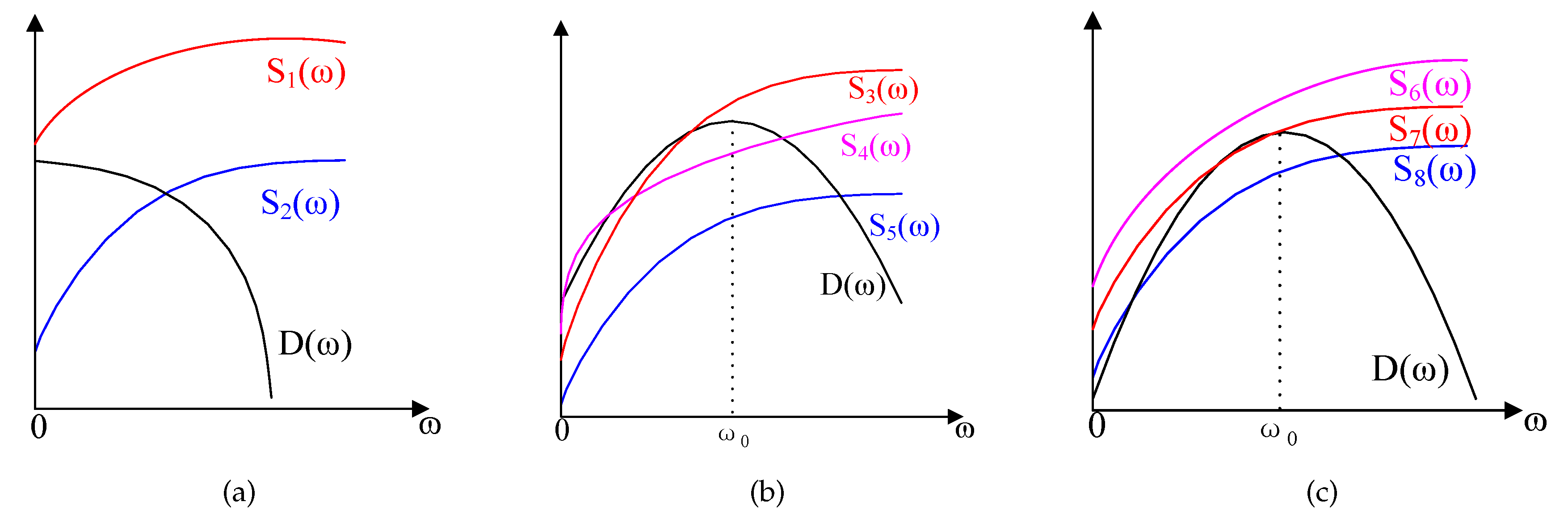
Since ${\sum }_{i\in N}{c}_i^{*}>0$ and $\partial S(\omega )/\partial \omega >0$, $S(\omega )$ is an increasing function. The relationships between $S(\omega )$ and $D(\omega )$ are described in Figure 3.

(a) When $G-p_0(N+1)<0$, we can obtain the following conclusions from Figure 3a:

• $S_1(\omega )$ (excessive supply): $p_0(\beta +{\beta }_0)p_s\ge p_{0}G/2h$, ${\omega }^{*}=0$,
• $S_2(\omega )$ (conservative supply): $p_0(\beta +{\beta }_0)p_s<p_{0}G/2h$, ${\omega }^{*}={\omega }_p$,

where ${\omega }_p$ is the intersection point of $D(\omega )$ and $S(\omega )$, and ${\omega }^{*}$ is the optimal parameter of the elastic price.

Because $p(c)$ is a linear rotational symmetric function, the case with ${\omega }^{*}=0$ is neglected.

(b) When $G-p_0(N+1)\ge 0$ and $p_0(\beta +{\beta }_0)p_s\ge p_{0}G/2h$, we have the conclusions by analyzing Figure 3b:

• $S_3(\omega )$ (excessive supply): $S_3(\omega )$ has one intersection with $D(\omega )$, where $D(\omega )$ has a non-negative slope, ${\omega }^{*}={\omega }_0$,
• $S_4(\omega )$ (conservative supply): $S_4(\omega )$ has three intersections with $D(\omega )$, ${\omega }^{*}={\omega }_p$,
• $S_5(\omega )$ (conservative supply): $S_5(\omega )$ has one intersection with $D(\omega )$, where $D(\omega )$ has a negative slope, ${\omega }^{*}={\omega }_p$.

(c) When $G-p_0(N+1)\ge 0$ and $p_0(\beta +{\beta }_0)p_s<p_{0}G/2h$, we can get the conclusions from Figure 3c:

• $S_6(\omega )$ (excessive supply): $S_6(\omega )$ doesn’t intersect with $D(\omega )$, ${\omega }^{*}={\omega }_0$,
• $S_7(\omega )$ (excessive supply): $S_7(\omega )$ has one or two intersections with $D(\omega )$, where both intersections are located in the increasing interval of $D(\omega )$, ${\omega }^{*}={\omega }_0$,
• $S_8(\omega )$ (conservative supply): $S_8(\omega )$ has two intersections with $D(\omega )$, where both intersections are located in the both sides of ${\omega }_0$, respectively, ${\omega }^{*}={\omega }_p$.

Letting $D(\omega )=S(\omega )$, we obtain a quadratic function with respect to $\omega$ and make it equal to zero:

$$\begin{array}{c}(G(N+1)+p_0{(N+1)}^2)(\beta +{\beta }_0)p_s{\omega }^2+[(4h{p}_0(N+1)+2hG)(\beta +{\beta }_0)p_s\hfill \\ -(G{p}_0(N+1)+G^2)]\omega +4h^2{p}_0(\beta +{\beta }_0)p_s-2h{p}_{0}G=0.\hfill \end{array}$$

(40)

For convenience, we define:

$$\begin{array}{cc}\hfill A& =G(N+1)+p_0{(N+1)}^2,\hfill \\ \hfill B& =4h{p}_0(N+1)+2hG,\hfill \\ \hfill C& =G{p}_0(N+1)+G^2,\hfill \\ \hfill D& =4h^2{p}_0,\hfill \\ \hfill E& =2h{p}_{0}G,\hfill \\ \hfill \Delta & =\sqrt{{(B(\beta +{\beta }_0)p_s-C)}^2-4A(\beta +{\beta }_0)p_s(D(\beta +{\beta }_0)p_s-E)}.\hfill \end{array}$$

Solving the above Equation (40), we obtain the intersection point of $D(\omega )$ and $S(\omega )$:

$$\begin{array}{cc}\hfill {\omega }_p& =\frac{-(B(\beta +{\beta }_0)p_s-C)+\Delta }{2A(\beta +{\beta }_0)p_s}.\hfill \end{array}$$

(41)

In the excessive supply regime, the maximum profit of the energy provider is at $\omega ={\omega }_0$:

$$\begin{array}{c}\hfill W_{II}^{ES}=\frac{{[G+p_0(N+1)]}^2}{8h(N+1)}-\mu {\beta }_0{p}_s-p_w\beta p_s.\end{array}$$

(42)

In the conservative supply regime, the maximum profit of the energy provider is at $\omega ={\omega }_p$:

$$\begin{array}{c}\hfill W_{II}^{CS}=\frac{(C-B(\beta +{\beta }_0)p_s+\Delta )G(\beta +{\beta }_0)p_s}{4Ah(\beta +{\beta }_0)p_s+(C-B(\beta +{\beta }_0)p_s+\Delta )(N+1)}+p_0(\beta +{\beta }_0)p_s-\mu {\beta }_0{p}_s-p_w\beta p_s.\end{array}$$

(43)

The optimal pricing decision and the corresponding optimal profit in Stage II are given in

Table 3. Optimal pricing decision and profit in Stage II in scenario B.

Total Energy Obtained	Optimal Parameter	Optimal Profit
in Stages I and II	${\mathit{p}}^{*}({\mathit{p}}_{\mathbf{s}},\mathit{\beta })$	${\mathit{W}}_{\mathbf{II}}({\mathit{p}}_{\mathbf{s}},\mathit{\beta })$
Excessive Supply Regime: $p_s\ge \frac{A}{4h(N+1)}$	${\omega }^{ES}={\omega }_0$	$W_{II}^{ES}(p_s,\beta )$ in Equation (43)
Conservative Supply Regime: $p_s<\frac{A}{4h(N+1)}$	${\omega }^{CS}={\omega }_p$	$W_{II}^{CS}(p_s,\beta )$ in Equation (44)

.

5.3. Energy Supply Strategy in Stage I

In Stage I, the energy provider also determines the energy purchase to maximize its profit by taking into account the uncertainty of the energy supply. The profit of the energy provider in the Stage I is given by:

$$\begin{array}{c}\hfill W_I=\underset{p_s\ge 0}{max}{W}_{II}(p_s,\beta ),\end{array}$$

(44)

where $W_{II}(p_s,\beta )$ is the energy provider’s profit function with respect to $p_s$ and the uncertain factor $\beta$ obtained in Stage II.

We assume that the wind power generation $P=\beta p_s$, and the minimum power and maximum power of the wind power generation are $P_{\min }$ and $P_{\max }$, respectively. The probability density function of the wind power $f_{WP}(P)$ can be obtained in [38]. From Figure 3, we can obtain that the maximum consumers’ demands ${\sum }_{i\in N}{c}_i^{*}(\omega )$ is $A/4h(N+1)$ when $\omega ={\omega }_0$. For convenience, we assume that $L=A/4h(N+1)$ and consider the following two intervals:

(1)

Interval I: $p_s\in [0,\frac{A}{4h(N+1)}]$. In this interval, the energy provider’s profit function is:

$$\begin{array}{cc}\hfill W_{II}^{1^{\prime }}(p_s)=& \hfill E_{P\in [P_{\min },P_{\max }]}\left[W_{II}^{CS}(P)\right]\\ \hfill =& \hfill {\int }_{P_{\min }}^{P_{\max }}{W}_{II}^{CS}(P)f_{WP}(P)\mathrm{d}P.\end{array}$$

(45)

(2)

Interval II: $p_s\in [\frac{A}{4h(N+1)},\infty ]$. The energy provider’s profit function is:

$$\begin{array}{cc}\hfill W_{II}^{2^{\prime }}(p_s)& =E_{P\in [P_{\min },\frac{A}{4h(N+1)}]}\left[W_{II}^{CS}(P)\right]+E_{P\in [\frac{A}{4h(N+1)},P_{\max }]}\left[W_{II}^{ES}(P)\right]\hfill \\ & ={\int }_{P_{\min }}^{\frac{A}{4h(N+1)}}{W}_{II}^{CS}(P)f_{WP}(P)\mathrm{d}P+{\int }_{\frac{A}{4h(N+1)}}^{P_{\max }}{W}_{II}^{ES}(P)f_{WP}(P)\mathrm{d}P.\hfill \end{array}$$

(46)

Similar to scenario A, we can obtain the maximum profit of the energy provider and the optimal amount of energy purchased from the electricity markets.

6. Simulation Results

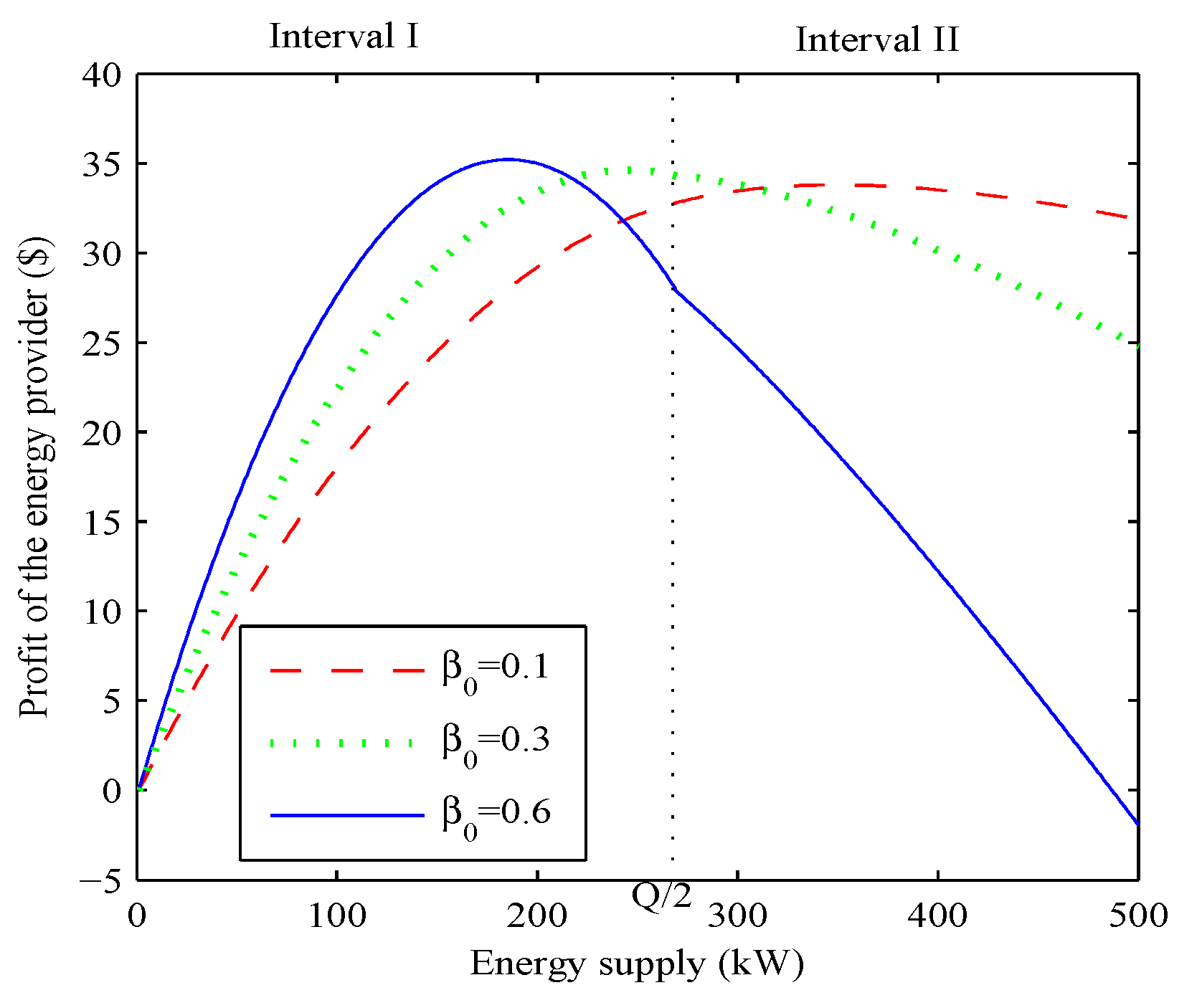
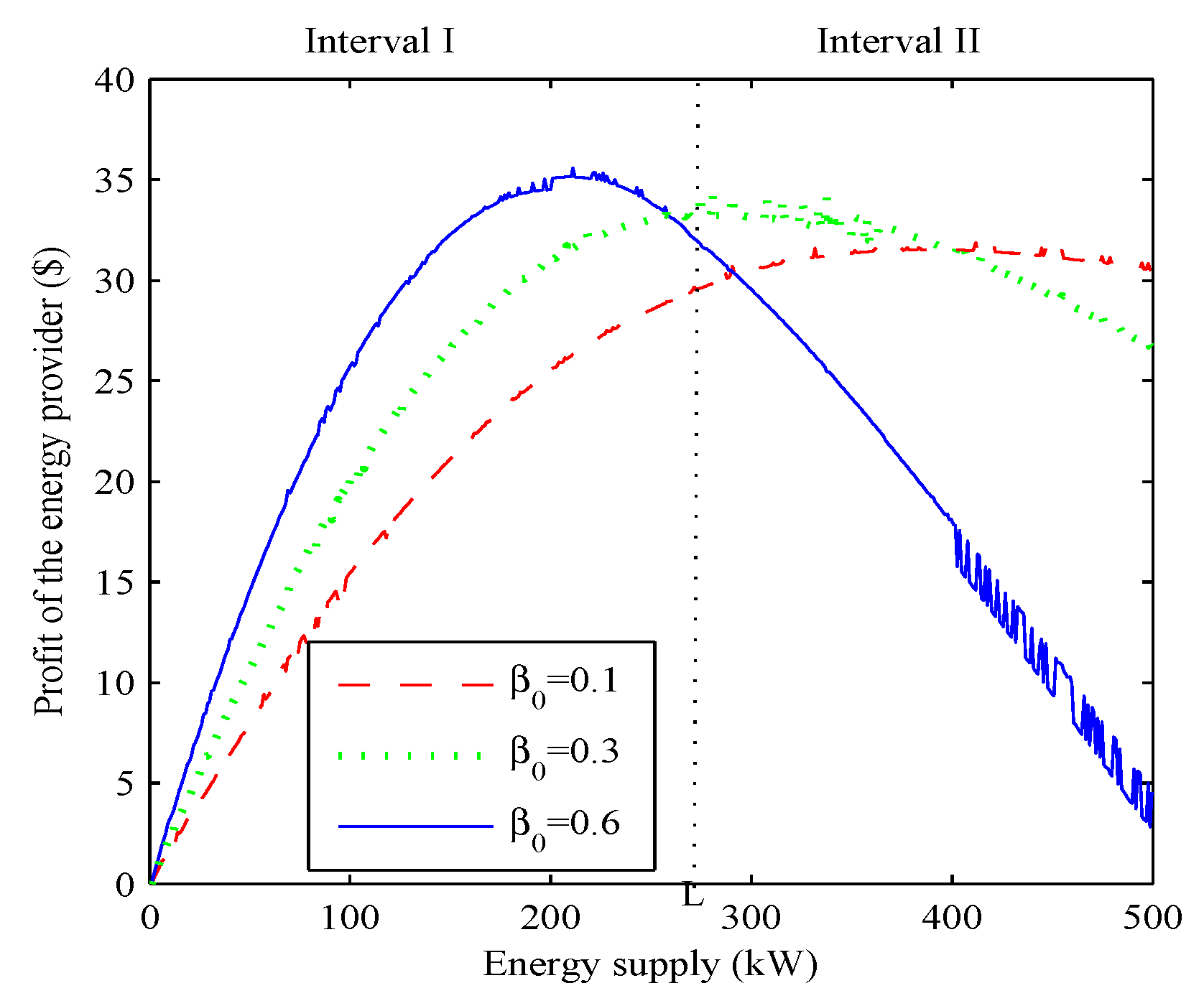
This section presents simulation studies of the proposed scheme using MATLAB 7.11.0 (MathWorks, Natick, MA, USA). In the simulations, we assume that the wind power generation follows a uniform distribution in $[P_{\min },P_{\max }]$, and we select that $h=0.04$, $p_0=0.1$, $N=100$, and $\mu =10$. For the parameter $c_i^{{}^{\prime }}$, we select a set of stochastic values. Then, we can obtain the profit of the energy provider under different ${\beta }_0$ for two scenarios as shown in Figure 4 and Figure 5, respectively.

From Figure 4 and Figure 5, we observe that the optimal energy supply decreases with the increase of the ${\beta }_0$ and the maximum profit is changed from Interval II to Interval I. In general, the wind power generation cost is less than the cost of purchasing energy. From the profit function of the energy provider, when ${\beta }_0$ increases, only by decreasing $p_s$ can the profit of the energy provider be maximized. Thus, it is verified that the proposed method is effective, and the simulation values of Figure 4 and Figure 5 are shown in

Table 4. Simulation values of the two scenarios.

	Scenario A		Scenario B
${\mathit{\beta }}_0$	${\mathit{p}}_{\mathbf{s}}$	Profit	${\mathit{p}}_{\mathbf{s}}$	Profit
0.1	349	33.79	399.6	31.52
0.3	246	34.61	288.6	33.27
0.6	186	35.2	209	35.13

.

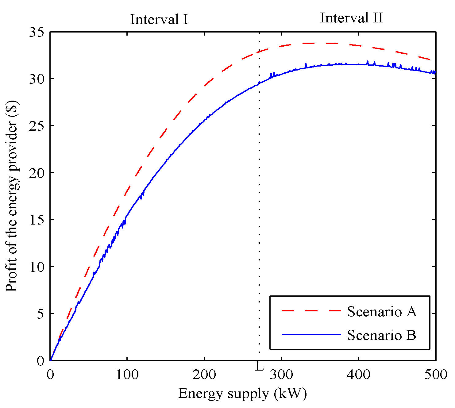
Taking ${\beta }_0=0.1$ as an example, the comparisons between the two scenarios are shown in Figure 6. From Figure 6 and Table 4, we observe that the energy provider can obtain more profit in scenario A.

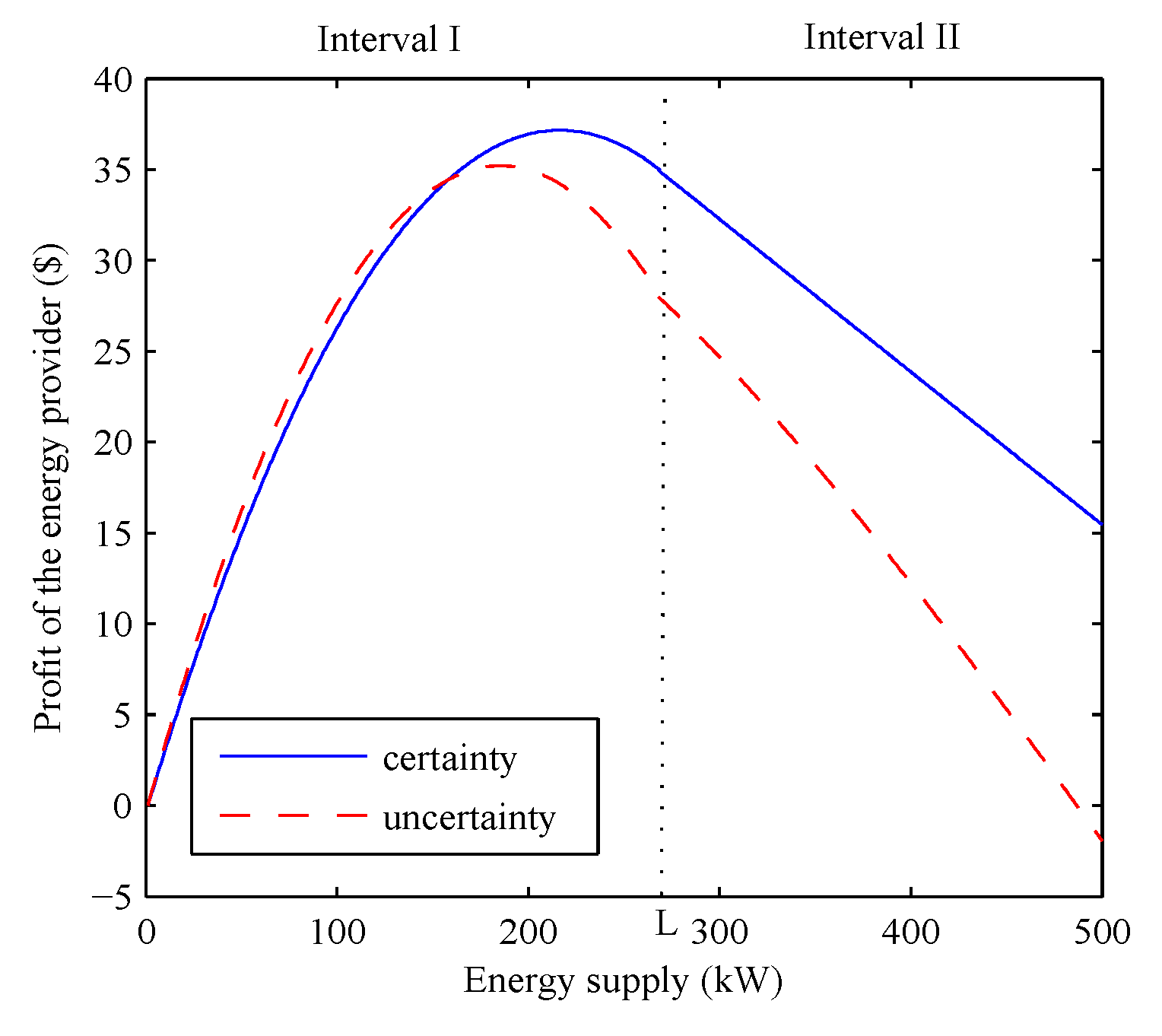
To explain the effect of the uncertainty, taking ${\beta }_0=0.6$ under scenario A as an example, we show the profit of the energy provider under the certain and uncertain energy supply in Figure 7. It is observed that the energy provider can achieve the higher profit under the certain energy supply. In reality, the uncertainty of the energy supply is necessary because the energy generated from the renewable energy sources is uncertain.

7. Conclusions

In this paper, we establish a model for energy trading and pricing in the microgrid. We formulate a hierarchical game between the energy provider with the renewable energy generation and the consumers, e.g., the price-taking consumers and the price-anticipating consumers. In the hierarchical game, the energy provider acts as the leader and the consumers act as the followers. The equilibrium point of the hierarchical game is obtained through the backward induction method. Furthermore, we also consider the uncertainty of the energy supply in the problem formulation. The simulation results show that the optimal energy supply can be obtained based on the reasonable pricing strategy and purchase strategy. Comparing the price-taking consumers with the price-anticipating consumers, we can obtain that the energy provider obtains more profit from the price-taking consumers. From the simulation results, we also can obtain that the energy provider’s profit reduces because of the uncertainty of the energy supply.

However, we do not consider that the consumers can sell the energy to the energy provider when the consumers have photovoltaic (PV) panels and a storage system. In that case, the energy demands of the consumers will be uncertain, and the payoff of the consumer includes two additional parts: one part is the PV generation cost, and the other part is the uncertainty of the energy demands. In order to compute the payoff of the consumer, we need to know the distribution that the PV generation follows. Then, we can get the average payoff of the consumer by expectation, and the optimal energy demands are obtained by the derivation method. Simultaneously, the profit of the energy provider needs to introduce two additional parts that denote buying the energy from the consumers and selling the energy to the electricity markets, which will be considered in the future.

References

- Chen, H.; Li, Y.; Han, Z.; Vucetic, B. A stackelberg game-based energy trading scheme for power beacon-assisted wireless-powered communication. In Proceedings of the IEEE International Conference on Acoustics, Speech and Signal Processing (ICASSP), Brisbane, Australia, 19–24 April 2015; pp. 3177–3181. [Google Scholar]
- Misra, S.; Bera, S.; Ojha, T.; Mouftah, H.T.; Anpalagan, A. ENTRUST: Energy trading under uncertainty in smart grid systems. Comput. Netw. 2016, 110, 232–242. [Google Scholar] [CrossRef]
- Belgana, A.; Rimal, B.P.; Maier, M. Open energy market strategies in microgrids: A Stackelberg game approach based on a hybrid multiobjective evolutionary algorithm. IEEE Trans. Smart Grid 2015, 6, 1243–1252. [Google Scholar] [CrossRef]
- Jia, L.; Tong, L. Dynamic pricing and distributed energy management for demand response. IEEE Trans. Smart Grid 2016, 7, 1128–1136. [Google Scholar] [CrossRef]
- Duan, L.; Huang, J.; Shou, B. Investment and pricing with spectrum uncertainty: A cognitive operator’s perspective. IEEE Trans. Mob. Comput. 2011, 10, 1590–1604. [Google Scholar] [CrossRef]
- Hu, M.C.; Lu, S.Y.; Chen, Y.H. Stochastic–multiobjective market equilibrium analysis of a demand response program in energy market under uncertainty. Appl. Energy 2016, 182, 500–506. [Google Scholar] [CrossRef]
- Nie, S.; Huang, C.Z.; Huang, G.H.; Li, Y.P.; Chen, J.P.; Fan, Y.R.; Cheng, G.H. Planning renewable energy in electric power system for sustainable development under uncertainty—A case study of Beijing. Appl. Energy 2016, 162, 772–786. [Google Scholar] [CrossRef]
- Ma, K.; Hu, G.; Spanos, C.J. Distributed energy consumption control via real-time pricing feedback in smart grid. IEEE Trans. Control Syst. Technol. 2014, 22, 1907–1914. [Google Scholar]
- Ma, K.; Hu, G.; Spanos, C.J. A cooperative demand response scheme using punishment mechanism and application to industrial refrigerated warehouses. IEEE Trans. Ind. Inform. 2015, 11, 1520–1531. [Google Scholar] [CrossRef]
- Mohsenian-Rad, A.H.; Wong, V.W.S.; Jatskevich, J.; Schober, R.; Leon-Garcia, A. Autonomous demand-side management based on game-theoretic energy consumption scheduling for the future smart grid. IEEE Trans. Smart Grid 2010, 1, 320–331. [Google Scholar] [CrossRef]
- Baharlouei, Z.; Hashemi, M.; Narimani, H.; Mohsenian-Rad, H. Achieving optimality and fairness in autonomous demand response: Benchmarks and billing mechanisms. IEEE Trans. Smart Grid 2013, 4, 968–975. [Google Scholar] [CrossRef]
- Yu, M.; Hong, S.H. Supply–demand balancing for power management in smart grid: A Stackelberg game approach. Appl. Energy 2016, 164, 702–710. [Google Scholar] [CrossRef]
- Gao, B.; Ma, T.; Tang, Y. Power transmission scheduling for generators in a deregulated environment based on a game-theoretic approach. Energies 2015, 8, 13879–13893. [Google Scholar] [CrossRef]
- Liu, N.; Wang, C.; Lin, X.; Lei, J. Multi-party energy management for clusters of roof leased PV prosumers: A game theoretical approach. Energies 2016, 9, 536. [Google Scholar] [CrossRef]
- Bu, S.; Yu, F.R. A game-theoretical scheme in the smart grid with demand-side management: Towards a smart cyber-physical power infrastructure. IEEE Trans. Emerg. Top. Comput. 2013, 1, 22–32. [Google Scholar] [CrossRef]
- Maharjan, S.; Zhu, Q.; Zhang, Y.; Gjessing, S. Dependable demand response management in the smart grid: A stackelberg game approach. IEEE Trans. Smart Grid 2013, 4, 120–132. [Google Scholar] [CrossRef]
- Soliman, H.M.; Leon-Garcia, A. Game-theoretic demand-side management with storage devices for the future smart grid. IEEE Trans. Smart Grid 2014, 5, 1475–1485. [Google Scholar] [CrossRef]
- Maharjan, S.; Zhu, Q.; Zhang, Y.; Gjessing, S.; Basar, T. Demand response management in the smart grid in a large population regime. IEEE Trans. Smart Grid 2016, 7, 189–199. [Google Scholar] [CrossRef]
- Lee, J.; Guo, J.; Choi, J.K.; Zukerman, M. Distributed energy trading in microgrids: a game-theoretic model and its equilibrium analysis. IEEE Trans. Ind. Electron. 2015, 62, 3524–3533. [Google Scholar] [CrossRef]
- Yoon, S.G.; Choi, Y.J.; Park, J.K.; Bahk, S. Demand response design based on a Stackelberg game in smart grid. In Proceedings of the International Conference on ICT Convergence, Jeju, Korea, 14–16 October 2013; pp. 177–178. [Google Scholar]
- Fadlullah, Z.M.; Quan, D.M.; Kato, N.; Stojmenovic, I. GTES: An optimized game-theoretic demand-side management scheme for smart grid. IEEE Syst. J. 2014, 8, 588–597. [Google Scholar] [CrossRef]
- Yang, B.; Li, J.; Han, Q.; He, T.; Chen, C.; Guan, X. Distributed control for charging multiple electric vehicles with overload limitation. IEEE Trans. Parallel Distrib. Syst. 2016, 27, 3441–3454. [Google Scholar] [CrossRef]
- Abegaz, B.W.; Mahajan, S.M. Optimal dispatch control of energy storage systems using forward-backward induction. In Proceedings of the 2015 International Conference on Clean Electrical Power (ICCEP), Taormina, Italy, 16–18 June 2015; pp. 731–736. [Google Scholar]
- Cho, J.; Kleit, A.N. Energy storage systems in energy and ancillary markets: A backwards induction approach. Appl. Energy 2015, 147, 176–183. [Google Scholar] [CrossRef]
- Mahoney, W.P.; Parks, K.; Wiener, G.; Liu, Y.; Myers, W.L.; Sun, J.; Monache, L.D.; Hopson, T.; Johnson, D.; Haupt, S.E. A wind power forecasting system to optimize grid integration. IEEE Trans. Sustain. Energy 2012, 3, 670–682. [Google Scholar] [CrossRef]
- Constantinescu, E.M.; Zavala, V.M.; Rocklin, M.; Lee, S.; Anitescu, M. A computational framework for uncertainty quantification and stochastic optimization in unit commitment with wind power generation. IEEE Trans. Power Syst. 2011, 26, 431–441. [Google Scholar] [CrossRef]
- Kanna, B.; Singh, S.N. Long term wind power forecast using adaptive wavelet neural network. In Proceedings of the 2016 IEEE Uttar Pradesh Section International Conference on Electrical, Computer and Electronics Engineering (UPCON), Varanasi, India, 9–11 December 2016; pp. 671–676. [Google Scholar]
- Xie, L.; Gu, Y.; Zhu, X.; Genton, M.G. Short-term spatio-temporal wind power forecast in robust look-ahead power system dispatch. IEEE Trans. Smart Grid 2014, 5, 511–520. [Google Scholar] [CrossRef]
- Finamore, A.R.; Galdi, V.; Calderaro, V.; Piccolo, A.; Conio, G.; Grasso, S. Artificial neural network application in wind forecasting: An one-hour-ahead wind speed prediction. In Proceedings of the 5th IET International Conference on Renewable Power Generation (RPG), London, UK, 21–23 September 2016; pp. 1–6. [Google Scholar]
- Sherlock, R.H. Analyzing winds for frequency and duration on atmospheric pollution. Am. Meteorol. Soc. 1951, 4, 42–49. [Google Scholar]
- Bardsley, W.E. Note on the use of the inverse Gaussian distribution for wind energy applications. J. Appl. Meteorol. 1980, 19, 1126–1130. [Google Scholar] [CrossRef]
- Luna, R.E.; Church, H.W. Estimation of long-term concentrations using a `universal’ wind speed distribution. J. Appl. Meteorol. 1974, 13, 910–916. [Google Scholar] [CrossRef]
- Hennessey, J.P.J. A comparison of the Weibull and Rayleigh distributions for estimating wind power potential. Wind Eng. 1978, 2, 156–164. [Google Scholar]
- Justus, C.G.; Hargraves, W.R.; Yalcin, A. Nationwide assessment of potential output from wind-powered generators. J. Appl. Meteorol. 1976, 15, 673–678. [Google Scholar] [CrossRef]
- Stewart, D.A.; Essenwanger, O.M. Frequency distribution of wind speed near the surface. J. Appl. Meteorol. 1978, 17, 1633–1642. [Google Scholar] [CrossRef]
- Takle, E.S.; Brown, J.M. Note on the use of Weibull statistics to characterize wind-speed data. J. Appl. Meteorol. 1978, 17, 556–559. [Google Scholar] [CrossRef]
- Liu, S.; Li, G.; Xie, H.; Wang, X. Correlation characteristic analysis for wind speed in different geographical hierarchies. Energies 2017, 10, 237. [Google Scholar] [CrossRef]
- Pan, X.; Wang, L.; Xu, Y.; Zhang, L.; Liu, W.; Wu, R. A wind farm power modeling method based on mixed Copula. Dianli Xitong Zidonghua/Autom. Electr. Power Syst. 2014, 38, 17–22. [Google Scholar]
- Du, M.; Yi, J.; Mazidi, P.; Cheng, L.; Guo, J. A parameter selection method for wind turbine health management through SCADA data. Energies 2017, 10, 253. [Google Scholar] [CrossRef]
- Ma, C. Robust exponential stability of reaction-diffusion generalized Cohen-Grossberg neural networks with distributed delays. J. Xinjiang Norm. Univ. 2007, 26, 18–24. [Google Scholar]
- Li, X.M.; Shi, D.J. Research on dependence structure between shanghai and shenzhen stock markets. Appl. Stat. Manag. 2006, 25, 729–736. [Google Scholar]
- Hu, L. Dependence patterns across financial markets: A mixed copula approach. Appl. Financ. Econ. 2006, 16, 717–729. [Google Scholar] [CrossRef]
Figure 1.
The system structure of energy trading.
Figure 2.
The relationships between and .
Figure 3.
The relationships between and under the different conditions.
Figure 4.
Scenario A: the profit of the energy provider under different .
Figure 5.
Scenario B: the profit of the energy provider under different .
Figure 6.
Comparisons between Scenario A with Scenario B.
Figure 7.
The effect of the uncertainty of the energy supply.