Power Take-Off Simulation for Scale Model Testing of Wave Energy Converters

Abstract

Small scale testing in controlled environments is a key stage in the development of potential wave energy conversion technology. Furthermore, it is well known that the physical design and operational quality of the power-take off (PTO) used on the small scale model can have vast effects on the tank testing results. Passive mechanical elements such as friction brakes and air dampers or oil filled dashpots are fraught with nonlinear behaviors such as static friction, temperature dependency, and backlash, the effects of which propagate into the wave energy converter (WEC) power production data, causing very high uncertainty in the extrapolation of the tank test results to the meaningful full ocean scale. The lack of quality in PTO simulators is an identified barrier to the development of WECs worldwide. A solution to this problem is to use actively controlled actuators for PTO simulation on small scale model wave energy converters. This can be done using force (or torque)-controlled feedback systems with suitable instrumentation, enabling the PTO to exert any desired time and/or state dependent reaction force. In this paper, two working experimental PTO simulators on two different wave energy converters are described. The first implementation is on a 1:25 scale self-reacting point absorber wave energy converter with optimum reactive control. The real-time control system, described in detail, is implemented in LabVIEW. The second implementation is on a 1:20 scale single body point absorber under model-predictive control, implemented with a real-time controller in MATLAB/Simulink. Details on the physical hardware, software, and feedback control methods, as well as results, are described for each PTO. Lastly, both sets of real-time control code are to be web-hosted, free for download, modified and used by other researchers and WEC developers.

1. Introduction

Similarity of Froude number is widely relied upon as a scaling law for the estimation of full scale wave energy converter (WEC) dynamics from model scale WEC observations. Because the WEC dynamics are highly dependent on the power-take off (PTO) force, the choice of PTO at the experimental scale is also critical to ensuring dynamic similarity. Previous experimental studies of scale model WEC devices have used a variety of systems to emulate the reaction forces exerted by a PTO device. Because these small scale systems are not intended to convert the scale model mechanical power into the final power commodity (electricity, fresh water, etc.), these systems are referred to as PTO simulators.

The PTO simulator must provide user-definable forces, dynamically similar to full scale WEC PTOs, that are adjustable to meet the desired PTO control scheme (i.e., passive damping, reactive, latching, etc.). Given a geometric scale ratio of $\alpha$ between experimental model and full scale WECs, under Froude scaling, the power absorption scales with ${\alpha }^{3.5}$ net. With such sensitivity in the scaling law, power losses from forces that are not dynamically similar, such as friction and mechanical backlash, must be minimized because they will obfuscate the power absorption results [1].

Some studies have designed PTO simulators using passive elements, such as oil-filled dashpots and pneumatic dampers [2,3], even though the range and resolution of PTO force adjustability is limited. Flocard and Finnigan reported using only three PTO damping settings from a PTO simulator based on a rotational viscous dashpot [2]. Bailey and Bryden reported using only five PTO damping settings from a PTO simulator based on translational pneumatic dampers [3]. Pecher reported testing six PTO settings on a PTO simulator based on adjustable sliding friction [4]. Although the simplicity and low cost of passive element PTO simulators is attractive, these systems have limited test ranges and can not be adjusted in situ, and thus do not allow investigations of alternative or advanced PTO control schemes.

Actively controlled PTO simulators, on the other hand, enable investigations of a much wider range of possible PTO control schemes. Both Taylor and Mackay [5] and Lopes et al. [6] designed and fabricated PTO simulators based on eddy current brakes that enable PTO control strategies beyond passive damping. Another actively controlled PTO simulator concept, requiring less complex electro-mechanical design than eddy current based systems, are feedback controlled electric motors. Feedback controlled motors, now common as off-the-shelf products for automation applications, can provide an arbitrarily defined PTO force with high resolution and repeatability when used in conjunction with a real-time controller and suitable instrumentation. Example implementations, reported by Villegas and Van der Schaaf [7] and Zurkinden et al. [8], used linear motors controlled in real-time by a feedback loop with the process variable being PTO force. Actively controlled PTO simulators can also function as an actuator for experimental identification of hydrodynamic coefficients.

The objectives of this work are to demonstrate the utility of actively controlled PTO simulators by presenting two separate applications based on feedback controlled linear motors, and to present the methodology used in each application for other researchers to implement in their own work. In Section 2, a PTO simulator is used to apply optimal passive damping control on a two-body point absorber in regular waves. In Section 3, a PTO simulator is applied to a more advanced model predictive control strategy on a one-body point absorber WEC.

Within each section, each application is described in terms of the physical system, controller implementation and results. The PTO simulator hardware is the same in both applications; the reaction force is provided by a linear motor, a load cell provides force feedback, and laser position sensors and accelerometers measure the motion of the WEC. PTO simulators therefore have great versatility, since the same hardware can be used to simulate a variety of different PTO systems and can be applied to multiple WEC designs.

2. Application: Passive Damping Control of Two-Body Point Absorber

In this section, a PTO simulator that successfully provided optimum passive damping control for a 1:25 scale model self-reacting point absorber WEC [9] is described and discussed.

2.1. Methods

2.1.1. Physical System

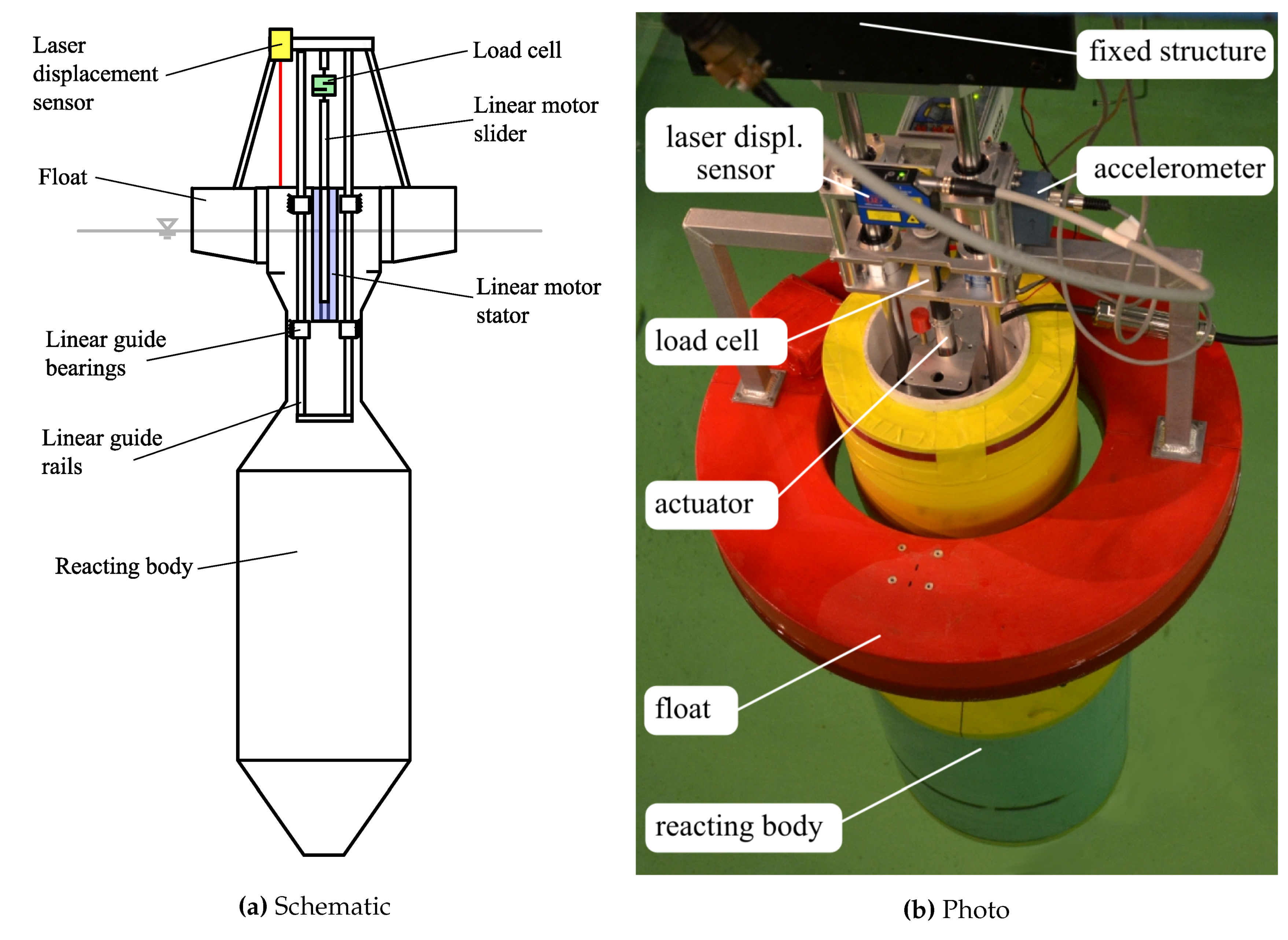
The PTO simulator consists of a linear motor and instrumentation connected between the float and reacting body of the experimental WEC model. A schematic of the system is given in Figure 1a and a photo of the system is given in Figure 1b.

The linear motor (LinMot PS01-37x120 by NTI AG, Spreitenbach, Switzerland), exerts 250 N maximum force, has a maximum travel of 0.28 m, and weighs under 3 kg. Relative displacements are measured with a non-contacting laser displacement sensor (optoNCDT-1402-600 by Micro-Epsilon, Ortenburg, Germany) with a range of 600 mm and resolution of 80 $\mu$m. The PTO force was measured by a 500 N capacity, S-type, tension/compression load cell. Accelerations of the float and reacting bodies were measured via accelerometers (ADXL203 by Analog Devices, Norwood,MA, USA) with +/−1.7 g range.

2.1.2. Reactive and Passive-Damping Control

The two-body WEC time-domain equations of motion, assuming heave motion only, can be modelled using a coupled system based on the Cummins Equation [10] with additional terms for the PTO force u and viscous drag $f_{dj}$:

$$\begin{array}{cc}\hfill M_1{\ddot{x}}_1\left(t\right)+{\int }_0^t{K}_1(t-\tau ){\dot{x}}_1\left(\tau \right)d\tau +k_1{x}_1\left(t\right)-f_{d1}\left(t\right)& =f_{e1}\left(t\right)-u\left(t\right),\hfill \\ \hfill M_2{\ddot{x}}_2\left(t\right)+{\int }_0^t{K}_2(t-\tau ){\dot{x}}_2\left(\tau \right)d\tau +k_2{x}_2\left(t\right)-f_{d2}\left(t\right)& =f_{e2}\left(t\right)+u\left(t\right),\hfill \end{array}$$

(1)

where $M_j=m_j+a_j\left(\infty \right)$ and $K_j\left(t\right)$ is the radiation impulse response function given by $K_j\left(t\right)=\frac{2}{\pi }{\int }_0^{\infty }b\left(\omega \right)cos\left(\omega t\right)d\omega$. The PTO force is defined as:

$$u=m_{pto}({\ddot{x}}_1-{\ddot{x}}_2)+c_{pto}({\dot{x}}_1-{\dot{x}}_2)+k_{pto}(x_1-x_2).$$

(2)

The relative velocity formulation of Morison drag is used for the drag forces $f_{d1}$ and $f_{d2}$ [9]. These can be linearized using an approach described by Clauss [11]. By carrying out this linearization of and assuming the regular incident waves, Equation (1) can be represented in the frequency domain as [12]:

$$ZU=F,$$

(3)

where $U={\left[{\widehat{U}}_1{\widehat{U}}_2\right]}^T$ are the complex amplitudes of body velocity, and $F={\left[X_1{\mathrm{e}}^{i{\Phi }_1}{X}_2{\mathrm{e}}^{i{\Phi }_2}\right]}^T$ are the complex excitation force amplitudes, and the impedance matrix Z is given by Equation (4). The hydrodynamic coupling impedance $Z_c$ is referred to as cross-radiation:

$$\begin{array}{cc}\hfill Z& =\left[\begin{array}{cc}{Z}_{11}+Z_{pto}& Z_c-Z_{pto}\\ Z_c-Z_{pto}& Z_{22}+Z_{pto}\end{array}\right],\hfill \\ \hfill Z_{jj}& =b_j\left(\omega \right)+i\omega \left(m_j+a_j\left(\omega \right)-\frac{k_j}{{\omega }^2}\right).\hfill \end{array}$$

(4)

Under reactive control, $Z_{pto}$ is free to have both real and imaginary terms, and the PTO acts as a coupling force with both passive and reactive contributions. In this case, power flows in two directions—power is not only absorbed by the PTO but also given back to the WEC from the PTO. This presents a challenging practical design problem for implementing full scale machines yet can enable large benefits to the overall WEC performance. In this case, optimum $Z_{pto}$ [12] is:

$$Z_{pto}^{reactive}=c_{pto}+i\omega \left(m_{pto}-\frac{k_{pto}}{{\omega }^2}\right)={\left(\frac{Z_{11}{Z}_{22}}{Z_{11}+Z_{22}}\right)}^{*}.$$

(5)

Under passive damping control, $Z_{pto}$ is constrained to be real valued, the PTO acts as a passive/resistive damping force with coefficient $c_{pto}$, and the optimum damping coefficient [12] is:

$$Z_{pto}^{passive}=c_{pto}=\left|\frac{Z_{11}{Z}_{22}}{Z_{11}+Z_{22}}\right|.$$

(6)

As is evident in Equations (5) and (6), the optimal values for $k_{pto}$, $c_{pto}$, and $m_{pto}$ are frequency dependent. Thus, on a WEC physical model:

• to physically realize reactive control, the PTO simulator must provide u with $k_{pto}$, $c_{pto}$, and $m_{pto}$ adjusted for each regular wave condition according to Equation (5).
• to physically realize passive damping control, the PTO simulator must provide u with $k_{pto},m_{pto}=0$ and $c_{pto}$ adjusted for each regular wave condition according to Equation (6).

The technical objective of the PTO simulator is to attain the greatest possible ranges for $k_{pto},m_{pto}=0$ and $c_{pto}$ to enhance the utility of this system. In practice, these ranges are limited by controller stability and the physical limitations of the linear motor.

2.1.3. Controller Implementation

The force output of the linear motor is determined by a controller implemented in NI LabVIEW and operated in real time on an NI PXI chassis running at 500 Hz for sampling and control. The purpose of the controller is to ensure the linear motor reaction force tracks the reference signal given in Equation (2). The controller minimizes the following error signal:

$$e\left(t\right)=f_{ref}-u,$$

(7)

where u is the measured PTO force and $f_{ref}$ is the reference signal defined as:

$$f_{ref}=m_{pto}{\ddot{\Delta }}_x+c_{pto}{\dot{\Delta }}_x+k_{pto}{\Delta }_x,$$

(8)

and ${\Delta }_x=x_1-x_2$ is the reference position of the WEC float relative to the reacting body.

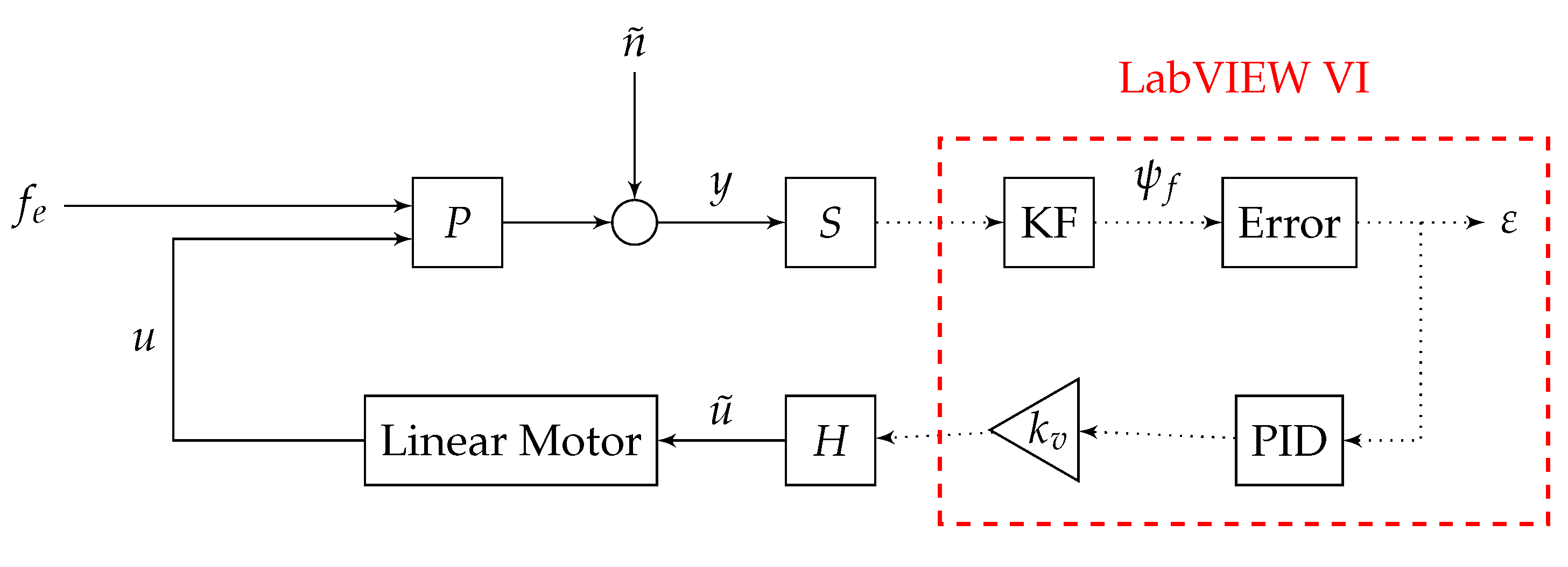
The reference signal is computed using measurements from the position sensor and accelerometers. A Kalman filter is used to synthesize the reference position, velocity and acceleration signals required to compute $f_{ref}$ via Equation (8). The PTO simulator can be represented by the following block diagram:

In Figure 2, S represents the sampling block, which converts the continuous-time measurements, y to discrete-time, and H represents the zero-hold operator, which converts the controller output from discrete-time to continuous-time. Signal $\epsilon$ represents the discrete-time equivalent of $e\left(t\right)$ given in Equation (7).

The transfer function P represents the dynamics of the WEC model. It provides the measurement signals y, which consists of the measurements provided by the laser sensor, accelerometers and load cell. These measurements are contaminated by sensor noise n before being sampled by the LabVIEW controller. LabVIEW then generates an analog control signal $\tilde{u}$ in Volts that is proportional to the force output of the linear motor. The gain between the linear motor force and the control signal $\tilde{u}$ is denoted as $k_v$. However, nonlinear forces due to friction and cogging [13] disturb the output force of the PTO; the purpose of the controller is to mitigate the error due to these effects.

The LabVIEW controller itself consists of three parts: a filter, an error signal calculator, and a proportional-integral-derivative (PID) feedback controller. The filter block applies a third-order Butterworth filter to each measurement in y. A Kalman Filter (KF) is then used to synthesize the reference position, velocity and acceleration signals required in Equation (8). The error block then uses the filtered signals to compute the discrete-time error signal $\epsilon$ based on Equation (7). Lastly, a PID controller is used to correct the output force of the linear motor to minimize the error signal. The PID controller was tuned in still water using the Ziegler–Nichols heuristic method resulting in a proportional term with gain 0.04, an integral term define by integral time 0.03 s, and zero derivative term.

2.1.4. State Space Model

A state-space model for P in Figure 2 can be derived starting with Equation (1) re-expressed as follows:

$$\begin{array}{cc}\hfill {\ddot{x}}_1& =\frac{1}{M_1}\left(f_{e1}-u+f_{r1}-k_1{x}_1-c_1{\dot{x}}_1\right),\hfill \\ \hfill {\ddot{x}}_2& =\frac{1}{M_2}\left(f_{e2}+u+f_{r2}-k_2{x}_2-c_2{\dot{x}}_2\right),\hfill \end{array}$$

(9)

where

$$f_{rj}\left(t\right)=-{\int }_0^t{K}_j(t-\tau ){\dot{x}}_j\left(\tau \right)d\tau .$$

(10)

Let $x_w={\left[\begin{array}{cccc}{x}_1& {\dot{x}}_1& x_2& {\dot{x}}_2\end{array}\right]}^T$ be a suitable vector of state variables for the system. Then, Equation (9) can be expressed as:

$${\dot{x}}_w={\mathbf{A}}_w^c{x}_w+{\mathbf{B}}_w^{c}f+{\mathbf{B}}_{wr}^c{f}_r,$$

where

$$f={\left[\begin{array}{ccc}{f}_{e1}& f_{e2}& u\end{array}\right]}^T,f_r={\left[\begin{array}{cc}{f}_{r1}& f_{r2}\end{array}\right]}^T,$$

$${\mathbf{A}}_w^c=\left[\begin{array}{cccc}0& 1& 0& 0\\ -{\displaystyle \frac{k_1}{M_1}}& -{\displaystyle \frac{c_1}{M_1}}& 0& 0\\ 0& 0& 0& 1\\ 0& 0& -{\displaystyle \frac{k_2}{M_2}}& -{\displaystyle \frac{c_2}{M_2}}\end{array}\right],$$

$${\mathbf{B}}_w^c=\left[\begin{array}{ccc}0& 0& 0\\ {\displaystyle \frac{1}{M_1}}& 0& -{\displaystyle \frac{1}{M_1}}\\ 0& 0& 0\\ 0& {\displaystyle \frac{1}{M_2}}& {\displaystyle \frac{1}{M_2}}\end{array}\right],{\mathbf{B}}_{wr}^c=\left[\begin{array}{cc}0& 0\\ {\displaystyle \frac{1}{M_1}}& 0\\ 0& 0\\ 0& {\displaystyle \frac{1}{M_2}}\end{array}\right].$$

The superscript c denotes that the state-space model is in the continuous domain. The output of P is the error signal given in Equation (11), which in terms of the inputs and state variables becomes:

$$\begin{array}{cc}\hfill e& =\frac{m_{pto}}{M_1}\left(f_{e1}-u+f_{r1}-k_1{x}_1-c_1{\dot{x}}_1\right)\hfill \\ & -\frac{m_{pto}}{M_2}\left(f_{e2}+u+f_{r2}-k_2{x}_2-c_2{\dot{x}}_2\right)\hfill \\ & +c_{pto}({\dot{x}}_1-{\dot{x}}_2)+k_{pto}(x_1-x_2)-u.\hfill \end{array}$$

(11)

The continuous-time state-space model for P can then be expressed as:

$$\begin{array}{cc}\hfill {\dot{x}}_w& ={\mathbf{A}}_w^c{x}_w+{\mathbf{B}}_w^{c}f+{\mathbf{B}}_{wr}^c{f}_r,\hfill \\ \hfill e& ={\mathbf{C}}_w^c{x}_w+{\mathbf{D}}_w^{c}f+{\mathbf{D}}_{wr}^c{f}_r,\hfill \end{array}$$

(12)

where

$${\mathbf{C}}_w^c=\left[\begin{array}{cccc}{k}_{pto}-{\displaystyle \frac{k_1{m}_{pto}}{M_1}}& c_{pto}-{\displaystyle \frac{c_1{m}_{pto}}{M_1}}& {\displaystyle \frac{k_2{m}_{pto}}{M_2}}-k_{pto}& {\displaystyle \frac{c_2{m}_{pto}}{M_2}}-c_{pto}\end{array}\right],$$

$${\mathbf{D}}_w^c=\left[\begin{array}{ccc}{\displaystyle \frac{m_{pto}}{M_1}}& -{\displaystyle \frac{m_{pto}}{M_2}}& -{\displaystyle \frac{m_{pto}}{M_1}}-{\displaystyle \frac{m_{pto}}{M_2}}-1\end{array}\right],$$

$${\mathbf{D}}_{wr}^c=\left[\begin{array}{cc}{\displaystyle \frac{m_{pto}}{M_1}}& -{\displaystyle \frac{m_{pto}}{M_2}}\end{array}\right].$$

An approximate state-space representation for the convolutions for $f_{r1}$ and $f_{r2}$ in Equation (10) can be obtained via the Hankel singular value decomposition [14]. Given the radiation impulse response function $K_j\left(t\right)$, the MATLAB function imp2ss.m [15] can approximate $f_{rj}$ as:

$$\begin{array}{cc}\hfill {\dot{x}}_{rj}& =A_{rj}{x}_{rj}+B_{rj}{\dot{x}}_j,\hfill \\ \hfill f_{rj}& =C_{rj}{x}_{rj}+D_{rj}{\dot{x}}_j.\hfill \end{array}$$

(13)

Note from Equation (13) that $f_{r1}$ and $f_{r2}$ can be expressed in terms of the state variable $x_w$ as:

$$\begin{array}{cc}\hfill {\dot{x}}_r& ={\mathbf{A}}_r^c{x}_r+{\mathbf{B}}_r^c{x}_w,\hfill \\ \hfill f_r& ={\mathbf{C}}_r^c{x}_r+{\mathbf{D}}_r^c{x}_w,\hfill \end{array}$$

(14)

where

$$\begin{array}{ccc}\hfill {\mathbf{A}}_r^c& =\left[\begin{array}{cc}{\mathbf{A}}_{r1}^c& 0\\ 0& {\mathbf{A}}_{r2}^c\end{array}\right],\hfill & {\mathbf{B}}_r^c=\left[\begin{array}{cccc}0& {\mathbf{B}}_{r1}^c& 0& 0\\ 0& 0& 0& {\mathbf{B}}_{r2}^c\end{array}\right],\hfill \\ \hfill {\mathbf{C}}_r^c& =\left[\begin{array}{cc}{\mathbf{C}}_{r1}^c& 0\\ 0& {\mathbf{C}}_{r2}^c\end{array}\right],\hfill & {\mathbf{D}}_r^c=\left[\begin{array}{cccc}0& {\mathbf{D}}_{r1}^c& 0& 0\\ 0& 0& 0& {\mathbf{D}}_{r2}^c\end{array}\right].\hfill \end{array}$$

Combining Equations (12) and (14) then gives the final state-space representation for P:

$$\begin{array}{cc}\hfill \dot{x}& ={\mathbf{A}}^{c}x+{\mathbf{B}}^{c}f,\hfill \\ \hfill e& ={\mathbf{C}}^{c}x+{\mathbf{D}}^{c}f,\hfill \end{array}$$

(15)

where the state variable is now $x={\left[\begin{array}{cc}{x}_w& x_r\end{array}\right]}^T$ and:

$$\begin{array}{cc}\hfill {\mathbf{A}}^c& =\left[\begin{array}{cc}{\mathbf{A}}_w^c+{\mathbf{B}}_{wr}^c{\mathbf{D}}_r^c& {\mathbf{B}}_{wr}{\mathbf{C}}_r^c\\ {\mathbf{B}}_r^c& {\mathbf{A}}_r^c\end{array}\right]\hfill \\ & =\left[\begin{array}{cccccc}0& 1& 0& 0& 0& 0\\ -{\displaystyle \frac{k_1}{M_1}}& {\displaystyle \frac{{\mathbf{D}}_{r1}^c-c_1}{M_1}}& 0& 0& {\displaystyle \frac{{\mathbf{C}}_{r1}^c}{M_1}}& 0\\ 0& 0& 0& 1& 0& 0\\ 0& 0& -{\displaystyle \frac{k_2}{M_2}}& {\displaystyle \frac{{\mathbf{D}}_{r2}^c-c_2}{M_2}}& 0& {\displaystyle \frac{{\mathbf{C}}_{r2}^c}{M_2}}\\ 0& {\mathbf{B}}_{r1}^c& 0& 0& {\mathbf{A}}_{r1}^c& 0\\ 0& 0& 0& {\mathbf{B}}_{r2}^c& 0& {\mathbf{A}}_{r2}^c\end{array}\right],\hfill \end{array}$$

$${\mathbf{B}}^c=\left[\begin{array}{c}{\mathbf{B}}_w^c\\ 0\end{array}\right]=\left[\begin{array}{ccc}0& 0& 0\\ {\displaystyle \frac{1}{M_1}}& 0& -{\displaystyle \frac{1}{M_1}}\\ 0& 0& 0\\ 0& {\displaystyle \frac{1}{M_2}}& {\displaystyle \frac{1}{M_2}}\\ 0& 0& 0\\ 0& 0& 0\end{array}\right],$$

$${\mathbf{C}}^c=\left[\begin{array}{cc}{\mathbf{C}}_w^c+{\mathbf{D}}_{wr}^c{\mathbf{D}}_r^c& {\mathbf{D}}_{wr}^c{\mathbf{C}}_r^c\end{array}\right]={\left[\begin{array}{c}{k}_{pto}-{\displaystyle \frac{k_1{m}_{pto}}{M_1}}\\ c_{pto}+({\mathbf{D}}_{r1}^c-c_1){\displaystyle \frac{m_{pto}}{M_1}}\\ {\displaystyle \frac{k_2{m}_{pto}}{M_2}}-k_{pto}\\ (c_2-{\mathbf{D}}_{r2}^c){\displaystyle \frac{m_{pto}}{M_2}}-c_{pto}\\ {\mathbf{C}}_{r1}^c{\displaystyle \frac{m_{pto}}{M_1}}\\ -{\mathbf{C}}_{r2}^c{\displaystyle \frac{m_{pto}}{M_2}}\end{array}\right]}^T,$$

$${\mathbf{D}}^c={\mathbf{D}}_w^c=\left[\begin{array}{ccc}{\displaystyle \frac{m_{pto}}{M_1}}& -{\displaystyle \frac{m_{pto}}{M_2}}& -{\displaystyle \frac{m_{pto}}{M_1}}-{\displaystyle \frac{m_{pto}}{M_2}}-1\end{array}\right].$$

The discrete-time realization $P_d$ can be obtained using the step-invariant transform [16]:

$$\begin{array}{cc}\hfill \dot{\xi }& =\mathbf{A}\xi +\mathbf{B}\zeta ,\hfill \\ \hfill \epsilon & =\mathbf{C}\xi +\mathbf{D}\zeta .\hfill \end{array}$$

(16)

The matrices $\mathbf{A}$, $\mathbf{B}$, $\mathbf{C}$ and $\mathbf{D}$ can be obtained using the MATLAB function c2d.m [15].

2.1.5. Stability Analysis

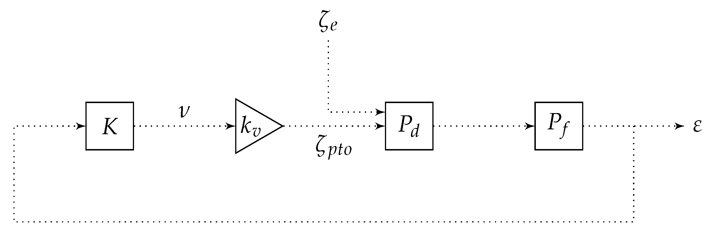
A stability analysis of the controller shown in Figure 2 can be done with a discrete-time simplified representation of the system shown in Figure 3. Signals ${\zeta }_e$, ${\zeta }_{pto}$ and $\nu$ are the discrete-time equivalents of $f_e$, u and u, respectively.

Referring to Figure 3, the discretized plant model is denoted $P_d$ as derived in Section 2.1.4. The output of $P_d$ is error signal given by Equation (7) directly, therefore eliminating the need to include the Kalman filter and error block from the original system. $P_f$ is the transfer function for a third-order Butterworth filter representing the delay observed in lab measurements. Finally, the linear motor transfer function is replaced by the gain $k_v$ neglecting nonlinearities such as friction or cogging. The PID controller is represented by K.

A MATLAB model [15] of the system in Figure 3 is used to analyze the stability properties by computing the pole locations of the transfer function between ${\zeta }_e$ and $\epsilon$.

2.1.6. Sensitivity to Noise

Since the reference force signal is dependent on the laser position sensor and accelerometers, care must be taken to ensure electrical noise is minimized as much as possible. It is particularly important when testing with large PTO coefficients, which amplify the measurement noise. While the lowpass filters and Kalman filter significantly reduce noise, some noise still carries through to the PID controller, decreasing the accuracy of the PTO emulation.

If ${\sigma }_x^2$ is the variance of the relative position output from the Kalman filter, while ${\sigma }_v^2$ and ${\sigma }_a^2$ are the corresponding variances for velocity and acceleration, then the variance of the reference force signal is:

$${\sigma }_{pto}^2=m_{pto}^2{\sigma }_a^2+c_{pto}^2{\sigma }_v^2+k_{pto}^2{\sigma }_x^2.$$

(17)

Therefore, it is expected that, in particular for tests with large $c_{pto}$, PTO performance may be significantly affected by sensor noise.

2.2. Results

2.2.1. Power Production Tests

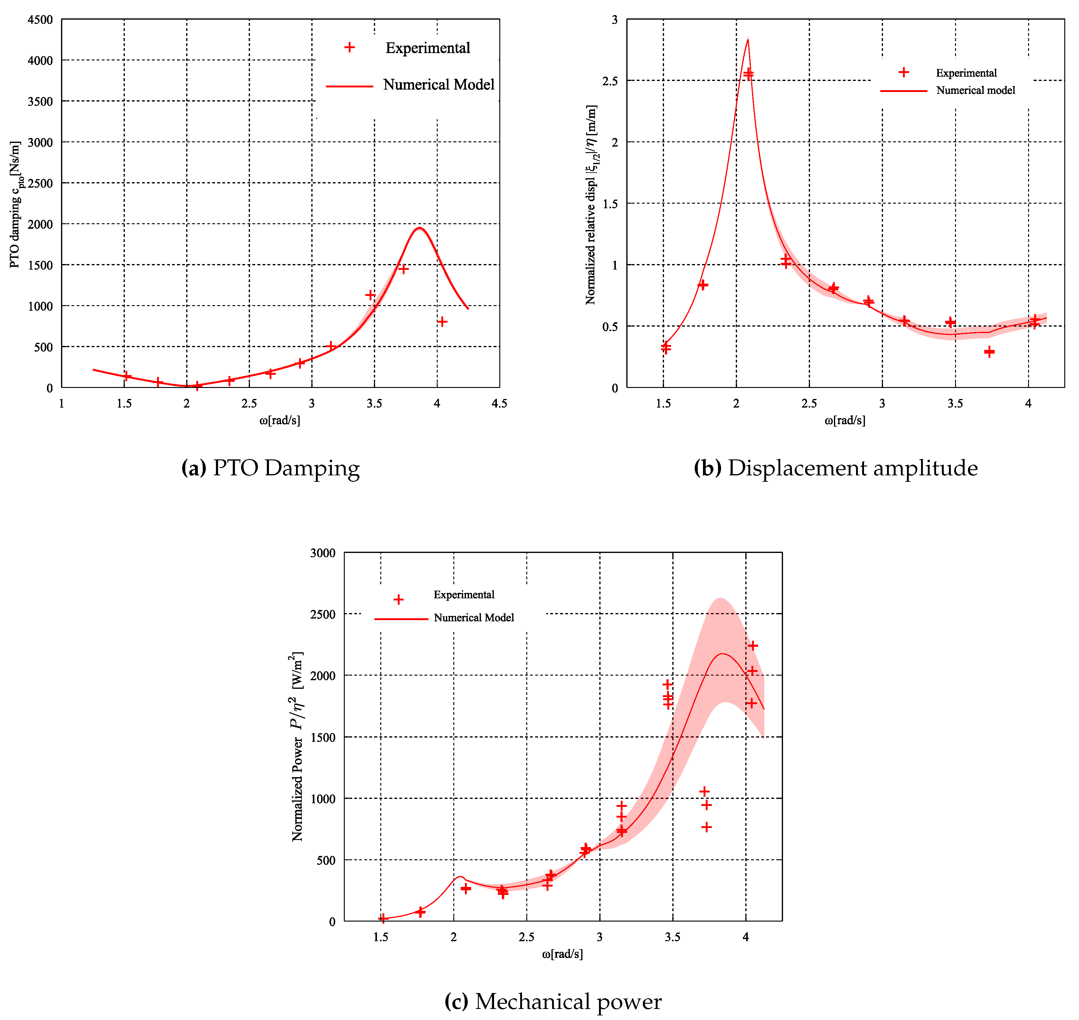
The PTO simulator was used to characterize the power production of the two-body point absorber, with optimal passive damping control in model tests with wave heights of 4–6 cm, frequencies $\omega$ = 1.5–4 rad/s. Frequency domain experimental displacement and mechanical power across the two-body point absorber PTO along with results from the numerical frequency domain model of Equation (3) are given in Figure 4.

Key points for the results of given in Figure 4 are as follows. For application to the experiments, the optimal passive damping PTO coefficients were estimated a priori by Equation (6) with boundary element methods (BEM). model estimates for the hydrodynamic terms feeding into $Z_{11}$ and $Z_{22}$; these $c_{pto}$ values are labelled “Experimental” in Figure 4a. Numerical model curves are a posteriori calculated using the model of Equation (3) with optimum damping given by Equation (6) including the best known set of hydrodynamic coefficients—a combination of numerically and experimentally derived coefficients. To indicate the sensitivity to uncertainty in hydrodynamic coefficients, the shaded regions of the model results are the envelope of the results from supplying Equation (3) with all possible combinations of experimental and BEM-derived hydrodynamic coefficients. The reader may refer to Beatty et al. [17] for a detailed description of the experimental methods and analysis.

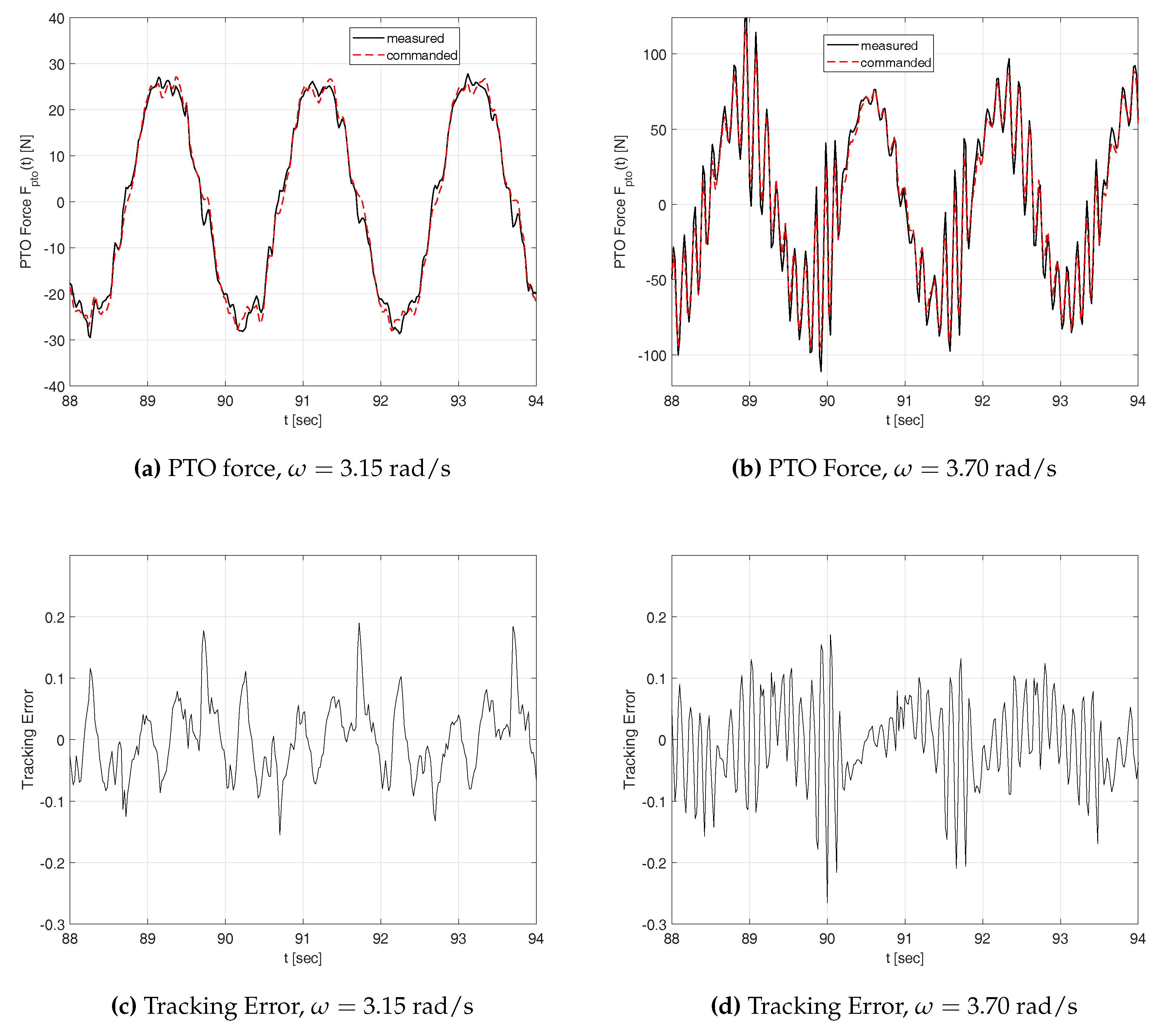
From Figure 4, it can be observed that the PTO simulator was generally successful for characterizing the performance of the two body WEC with optimal PTO damping, apart from the wave frequency $\omega =$ 3.7 rad/s where the controller exhibited poor performance. The poor controller performance resulted from a couple of factors. First, the wave frequency $\omega =$ 3.7 rad/s coincides with the peak of the WEC’s performance, and is thus demanding the greatest PTO force of all tests. Second, at $\omega =$ 3.7 rad/s, sensor noise contributed particularly large disturbances to the force reference signal in comparison to the tests at other wave frequencies. This is observed in the time series of the actual and reference PTO force given by Figure 5.

During most wave conditions, the PTO simulator showed reasonable capability to track the reference force; however, at wave frequencies around $\omega =3.7$ rad/s, a drop in controller performance was encountered. Figure 5b shows the actual and reference forces signals while the control system introduced high amplitude, higher frequency oscillations into the system. Figure 5c,d show the time series for the error between the measured and reference force signals, normalized by the amplitude of the reference signal. Figure 5e shows the variance of force oscillations related to the control instability for each test, indicating that the instability is localized around $\omega$ = 3.5–4.1 rad/s. This range of frequencies corresponds with the highest levels of the optimal $c_{pto}$ coefficient, where noise in the velocity measurement is greatly amplified. This illustrates the importance of reducing measurement noise as much as possible to obtain a cleaner reference force signal and improve PTO simulation.

2.2.2. Stability

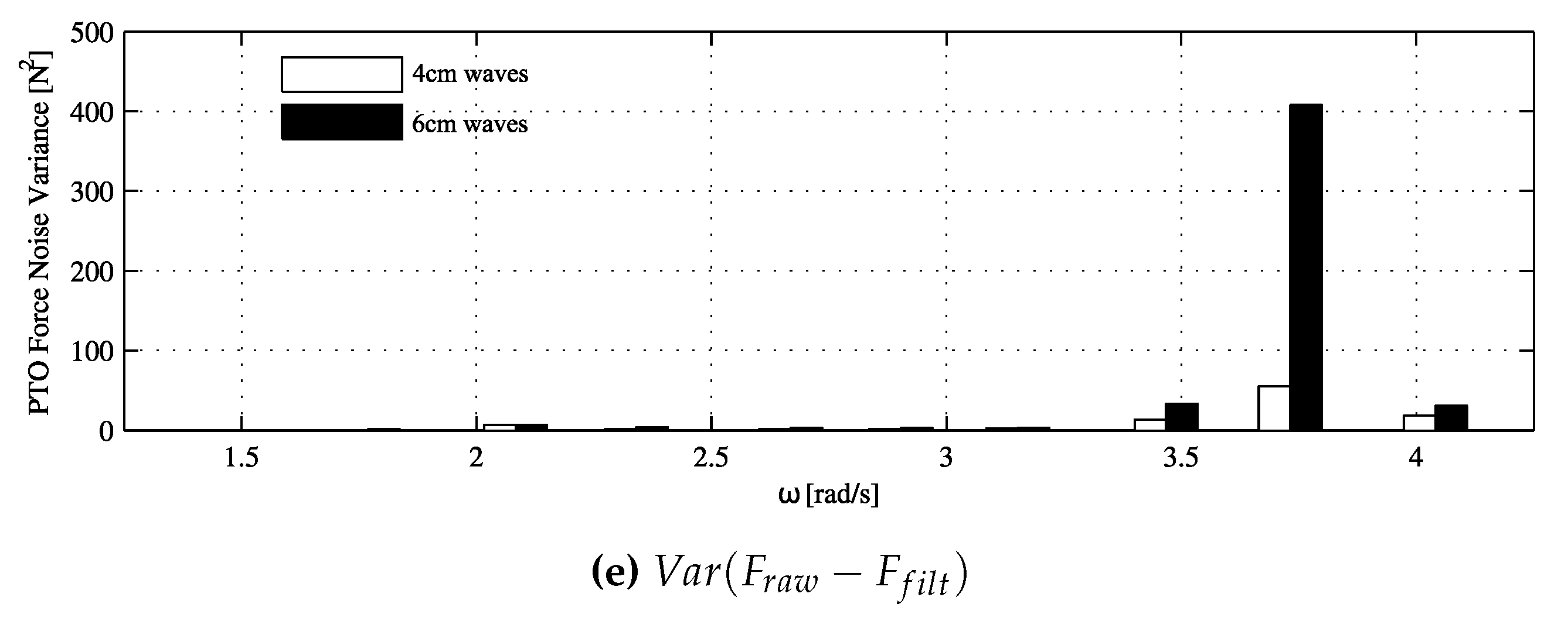
To investigate the stability issue encountered around $\omega =3.70$ rad/s, a stability analysis of the controller shown in Figure 3 was done using the methods discussed in Section 2.1.5. Figure 6a shows the pole locations for increasing values of $c_{pto}$, while $m_{pto}=k_{pto}=0$ as a representative of the experimental tests. Since none of the poles fall outside the unit circle, the system is theoretically stable for the high ranges of $c_{pto}$. Thus, the issue observed around $\omega$ = 3.5–4.1 rad/s may be attributed to sensor noise, rather than an unstable control system.

Because the PTO simulation methods described in this section can be applied to reactive control scenarios (i.e., $k_{pto}\ne 0$ and/or $m_{pto}\ne 0$), the controller stability analysis is extended here to those other scenarios. Figure 6b shows the pole locations for increasing values of $k_{pto}$, while $c_{pto}=m_{pto}=0$. Figure 6c shows the pole locations for increasing values of $m_{pto}$, while $c_{pto}=m_{pto}=0$.

From Figure 6b–d, it can be observed that some combinations of PTO coefficients will result in an unstable system. Figure 6a–c show that the system is stable for wide ranges of individually set $c_{pto}$ and $m_{pto}$ but can transition to unstable for high individual values of $k_{pto}$. Figure 6d shows how increasing $c_{pto}$ can stabilize an otherwise unstable system with $k_{pto}=5000$ N/m. Thus, during implementation of these methods, the reader is cautioned to re-tune the controller settings for individual combinations of PTO coefficients.

2.3. Discussion

A PTO simulation methodology for testing a two body WEC with optimum passive damping in regular waves has been demonstrated. The hardware and instrumentation as well as the controller architecture has been described. The PTO simulator performed its intended function generally, apart from poor performance observed at a specific frequency range within the test regime, which is attributed to sensor noise. In addition, a stability analysis of the control architecture indeed shows specific vulnerability to instability in certain combinations of PTO coefficients. Recommended improvements to the control architecture are as follows:

• Provide the force reference signal as a feed-forward term in the linear motor control signal, for example as implemented by Villegas and van der Schaaf [7]. This minimizes the magnitude of the control actions, as the PID controller is required only to cancel disturbance forces.
• Include PTO joint friction and linear motor cogging as feedforward forces.
• Include a correction to the PTO force due to the acceleration of the reference frame.

The next section details the application of the PTO simulation strategy to optimal model-predictive control of a single body WEC in irregular waves.

3. Application: Model Predictive Control of One-Body Point Absorber

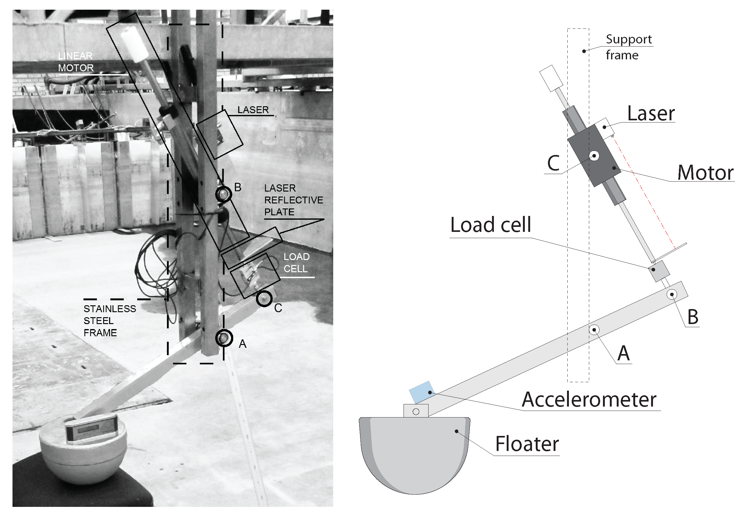
This section highlights the implementation and test of a model predictive control (MPC) applied to a 1:20 scale physical model single absorber from the Wavestar WEC. The Wavestar WEC is a bottom-mounted multi-absorber WEC [18]. Each absorber is a single degree-of-freedom (DOF), wave-activated body system composed of a hinged arm and a floater. The single DOF floater motion is the rotation about the pivot point (A). An image of the physical model and a schematic sketch are given in Figure 7.

3.1. Physical System

The PTO system is composed of a linear motor connecting a reference inertial frame to the absorber, suitable instrumentation, and a real-time controller.

A summary of the PTO instrumentation is as follows:

• Position sensor: Laser displacement sensor and reflective laser surface: MicroEpsilon ILD-1402-600.
• Acceleration sensor: Dual-axis accelerometer, Analog Devices ADXL203EB.
• Force sensor: Extension-compression s-beam load cell, Futek LSB302 300lb, with SGA Analogue Strain Gauge Amplifier.
• Actuator: Linear DC two phase brushless motor, LinMot Series P01-37x240, equipped with LinMot controller Series E1100.

The floater diameter is 0.25 m at the equilibrium waterline. The natural frequency of the floater is approx 0.8 s at model scale. The PTO force is constrained in the range $\pm 200$ N in order to guarantee a safe operation of the machine.

3.2. Model Predictive Control

To generate an optimal reference force signal for the physical model PTO, a control architecture relating the system state to an optimal target force must be implemented. In the first PTO simulation application, outlined in Section 2, the PTO reference force is generated by multiplication of the system state with constant PTO coefficients, which has applicability limited to idealized scenarios and results in lower WEC performance in irregular waves. By contrast, this section outlines a model predictive control (MPC) method to generate an optimal target force signal in the time domain enabling optimized performance of the single wavestar point absorber in irregular waves.

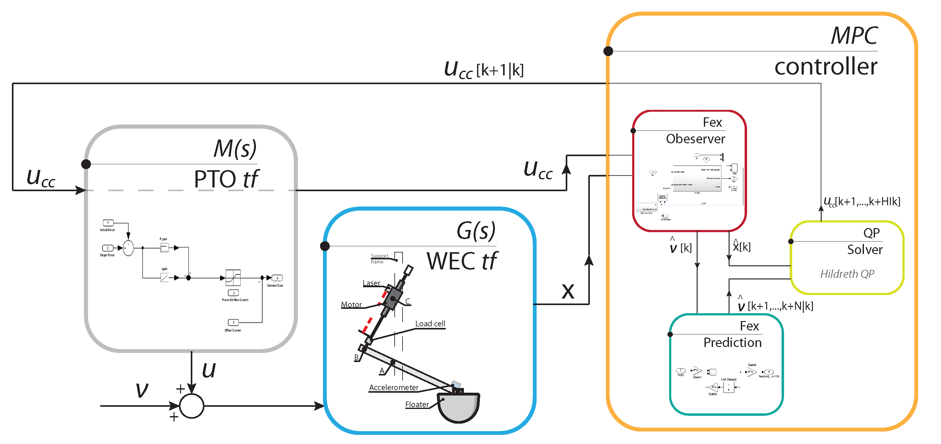
Figure 8 shows a block-diagram for the system and the controller model.

3.2.1. PTO and WEC Models

The commanded target force ($u_{cc}$) is passed through the linear actuator transfer function ($M\left(s\right)$) to generate the actual target force (u). u is summed with the wave excitation force ($\nu$) and fed to the transfer function of the WEC ($G\left(s\right)$), resulting in the WEC dynamic state (x). The dynamic state space model of the linear actuator, including the actuator controller, depends on the machinery type, orientation, etc.; therefore, an a priori model cannot be generalized. This dynamic model can be obtained in several ways, such as simplified transfer function from data sheet parameters, model fitting of input/output data, etc.

To model the WEC, we apply a state-space model derived from the familiar Cummins equations by Yu and Falnes [19]:

$$\begin{array}{ccc}\hfill {\dot{x}}_p^c& =& {\mathbf{A}}_p^c{x}_p^c+{\mathbf{B}}_p^c(\nu +u),\hfill \\ \hfill v^c& =& {\mathbf{C}}_{\mathbf{p}}^{\mathbf{c}}{x}_p^c,\hfill \end{array}$$

(18)

where:

$$\begin{array}{ccc}\hfill {\mathbf{A}}_p^c& =& \left[\begin{array}{ccc}0& 1& \underline{0}\\ -K/J_{tot}& -{\mathbf{D}}_{\mathbf{r}}^{\mathbf{c}}/J_{tot}& -{\mathbf{C}}_{\mathbf{r}}^{\mathbf{c}}/J_{tot}\\ \underline{0}& {\mathbf{B}}_{\mathbf{r}}^{\mathbf{c}}& {\mathbf{A}}_{\mathbf{r}}^{\mathbf{c}}\end{array}\right],\hfill \\ \hfill {\mathbf{B}}_p^c& =& \left[\begin{array}{c}0\\ 1/J_{tot}\\ \underline{0}\end{array}\right],\hfill \\ \hfill {\mathbf{C}}_p^c& =& \left[\begin{array}{ccc}0& 1& \underline{0}\end{array}\right],\hfill \\ \hfill x_p^c& =& {\left[\begin{array}{ccc}\theta & \dot{\theta }& x_r\end{array}\right]}^T,\hfill \end{array}$$

(19)

$$\begin{array}{ccc}\hfill v^c& =& \dot{\theta }.\hfill \end{array}$$

(20)

Superscript c identifies a continuous time model; p denotes the state-space model of the $\underline{p}$lant; m denotes the model of the $\underline{m}$achine; K is the hydrostatic stiffness; $J_{tot}$ is the total mass moment of inertia of the system; ${\mathbf{A}}_{\mathbf{r}}^{\mathbf{c}}$, ${\mathbf{B}}_{\mathbf{r}}^{\mathbf{c}}$, ${\mathbf{C}}_{\mathbf{r}}^{\mathbf{c}}$ and ${\mathbf{D}}_{\mathbf{r}}^{\mathbf{c}}$ are the state-space matrices of the radiation model, $\theta$ and $\dot{\theta }$ are the angular position and velocity, respectively, and $x_r$ is the radiation state vector. The total mass moment of inertia is obtained from the summation of the mass moment of inertia of the dry system and the added mass at infinite frequency.

Since the MPC will be implemented in a digital machine, it is required to discretize the PTO and WEC models prior to the controller formulation. To this end, the bi-linear transform is applied according to the MPC implementation presented in [20].

The discrete state-space model of the plant is defined as:

$$\begin{array}{ccc}\hfill x[k+1]& =& \mathbf{A}x\left[k\right]+\mathbf{B}\left(\nu \right[k]-u[k\left]\right),\hfill \\ \hfill v\left[k\right]& =& \mathbf{C}x\left[k\right]+\mathbf{D}\left(\nu \right[k]-u[k\left]\right).\hfill \end{array}$$

(21)

Here, k identifies the time index (integer) and $\mathbf{A}$, $\mathbf{B}$, $\mathbf{C}$ and $\mathbf{D}$ are the state-space matrices of the system. The matrix $\mathbf{D}$ identifies the constant term of a proper transfer function decomposition. It arises from the non-strictly proper representation of the continuous system returned by the bi-linear transform. It should be noted that the discrete state-space model of the PTO has a very similar shape to Equation (23).

In order to formulate an MPC for the state space system given by (18)–(23), it is necessary to forecast the system dynamics over the future N samples. The MPC formulation is thus comprised of the following three key blocks:

• Excitation Force Observer,
• Excitation Force Prediction,
• Quadratic Problem Solver.

3.2.2. Excitation Force Observer

The prediction of the system velocity is linked to the excitation force measurements/forecast over the entire prediction horizon. The excitation force is not directly measurable, and its actual value requires estimation using a soft-sensor observer technique.

The observation of the state is achieved by combining a model of the system (18) with measurements of system state and forces. If the system is linear, or can be linearized, a Kalman observer guarantees the minimum observation error of the state in a linear sense, [21]. Taking advantage of this fact, a linear Kalman observer is applied here using the numerical model of the plant WEC and PTO along with real-time state measurements from the sensors.

3.2.3. Excitation Force Prediction

Once an estimation of the excitation force is available, it is possible to predict its evolution over the prediction horizon required by the controller using an auto-regressive model (AR). Other models are possible but as presented in several works [22,23], AR has clear advantages over the other tested candidates.

An AR model assumes a linear correlation between the past and future values of the variable. Therefore, the one-step ahead predictor can be defined as:

$$\widehat{\nu }[k+1|k]=\sum _{i=0}^{n-1}{a}_i·\nu [k-i],$$

(22)

where $\widehat{\nu }[k+1|k]$ is the predicted excitation force at time $k+1$ given the state of the variable at time k, n is the model order, $a_i\left[k\right]$ are the model coefficients and $\nu [k-i]$ is a scalar in the vector containing the past values of the estimated excitation force. Numerical and physical implementations of the AR model for the prediction of the excitation force are presented in [24,25,26]. The multi-step ahead prediction can be obtained using the plug-in or sequential method, in which the predicted step ($k+1$) is pre-pended at the vector of past values of the excitation force.

The coefficients of the AR model are assessed by minimizing the squared error between the predicted values and measured values. The excitation force time series is measured by generating waves while the structure is held fixed in its equilibrium position.

Since the AR coefficients are fitted to a specific sea state, they should be updated whenever the sea state changes. However, by laboratory experience, it has been noticed that, for the tested sea state, the influence of AR model variation was marginal; therefore, in this work, $a_i\left[k\right]$ are held fixed in time. Note that the prediction technique has a direct influence on the controller capability. Refer to [22,27] for general considerations on this matter.

3.2.4. Quadratic Program Formulation

Define the prediction vector as:

$$\begin{array}{c}\hfill \underline{\mathbf{\varnothing }}\left[k\right]={\left[\chi [k+1|k],\cdots ,\chi [k+N\left|k\right]\right]}^T.\end{array}$$

The target force u and system velocity v can be obtained over the prediction horizon from the free evolution of the state-space model:

$$\begin{array}{ccc}\hfill \underline{\mathbf{u}}\left[k\right]& =& {\mathcal{P}}_m{x}_m\left[k\right]+{\mathcal{T}}_m{\underline{\mathbf{u}}}_{cc}\left[k\right],\hfill \end{array}$$

(23)

$$\begin{array}{ccc}\hfill \underline{\mathbf{v}}\left[k\right]& =& {\mathcal{P}}_p{x}_p\left[k\right]+{\mathcal{T}}_p(\underline{\nu }\left[k\right]-\underline{\mathbf{u}}\left[k\right])\hfill \end{array}$$

(24)

$$\begin{array}{cc}=& {\mathcal{P}}_{pm}+{\mathcal{T}}_{pm}{\underline{\mathbf{u}}}_{cc}\left[k\right],\hfill \end{array}$$

(25)

where:

$$\begin{array}{ccc}\hfill \mathcal{P}& =& \left[\begin{array}{c}\mathbf{CA}\\ {\mathbf{CA}}^2\\ ⋮\\ {\mathbf{CA}}^N\end{array}\right],\hfill \end{array}$$

$$\begin{array}{ccc}\hfill \mathcal{T}& =& \left[\begin{array}{ccccc}\mathbf{D}& \underline{0}& \underline{0}& \cdots & \underline{0}\\ \mathbf{CB}& \mathbf{D}& \underline{0}& \cdots & \underline{0}\\ \mathbf{CAB}& \mathbf{CB}& \mathbf{D}& \cdots & \underline{0}\\ ⋮& ⋮& ⋮& \ddots & ⋮\\ {\mathbf{CA}}^{N-1}\mathbf{B}& {\mathbf{CA}}^{N-2}\mathbf{B}& {\mathbf{CA}}^{N-3}\mathbf{B}& \cdots & \mathbf{D}\end{array}\right].\hfill \end{array}$$

The subscripts have been omitted from the definition above for simplicity and $\underline{0}$ has to be considered as a zero matrix with the same shape as $\mathbf{D}$. Equation (25) is obtained by substituting Equation (23) in Equation (24), and by separating the terms proportional to and independent of the commanded target force.

The objective of the controller is to minimize the objective function (J) over the prediction horizon, within a (given) feasible region, by varying the controller load. Using the receding control theory only the first sample of the predicted control trajectory is implemented, and, at each time step, a full optimization problem is solved.

In this work, the cost function considers absorbed energy only, but other alternatives are possible [24]. The cost function is formally defined as the mechanical energy absorbed by the WEC over the prediction horizon using an Euler integration scheme:

$$\begin{array}{c}\hfill J={\int }_t^{t+N\delta T}u\left(\tau \right)v\left(\tau \right)d\tau \underset{Continuos}{\overset{Discrete}{\iff }}\underline{\mathbf{u}}{\left[k\right]}^T·\underline{\mathbf{v}}\left[k\right],\end{array}$$

(26)

where “·” is the vector dot product, t is the actual instant of time, and $\delta T$ is the time step between two successive samples. To form the optimization as a quadratic programming problem, Equation (25) and Equation (23) are substituted into Equation (26):

$$\begin{array}{ccc}\hfill J& =& \frac{1}{2}{\underline{\mathbf{u}}}_{cc}^T\mathbf{Q}{\underline{\mathbf{u}}}_{cc}+\mathbf{f}{\underline{\mathbf{u}}}_{cc}+c_o,\hfill \end{array}$$

(27)

where:

$$\begin{array}{ccc}\hfill \mathbf{Q}& =& {\mathcal{T}}_{pm}^T{\mathcal{T}}_m^T+{\mathcal{T}}_m{\mathcal{T}}_{pm},\hfill \\ \hfill \mathbf{f}& =& {\mathcal{P}}_{pm}^T{\mathcal{T}}_m+x_m^T{\mathcal{P}}_m^T{\mathcal{T}}_{pm},\hfill \\ \hfill c_o& =& x_m^T{\mathcal{P}}_m^T{\mathcal{P}}_{pm}.\hfill \end{array}$$

The convexity of the cost function given in Equation (26) is not guaranteed. As presented in [28,29], the convexity can be imposed by adding a penalties term proportional to the target force and its variation.

3.2.5. Controller Implementation

On the Wavestar physical scale model, the target force commanded by the MPC algorithm input to the real-time controlled PTO simulator. The PTO simulator is comprised of a real-time control application, the LinMot linear motor, and the LinMot E1100 controller. The MPC is implemented using a Simulink block diagram on a host PC. The host PC is interfaced with a second PC that runs a kernel of xPC Target via TCP/IP connection. The xPC target runs the MPC controller in real time and communicates with the physical model and the LinMot via an NI PCI-6221 IO interface. The target force signal is generated at a sample rate of 1 kHz. The real-time controller seeks to minimize the error between the target and measured forces. The real-time controller used is the built-in PI force control architecture within the LinMot E1100. The overall control architecture is shown in Figure 8 and the LinMot force PI controller parameters are summarized in

Table 1. LinMot set-up description and controller parameters.

Name		Value
Description	Parameter
Analog Input on LinMot board, force measurement	x4.4	−
Analog Input on LinMot board, force target	x4.7	−
Proportional coefficient	$K_p$	$0.5$
Integral coefficient	$K_i$	$1.47$

.

3.3. Results

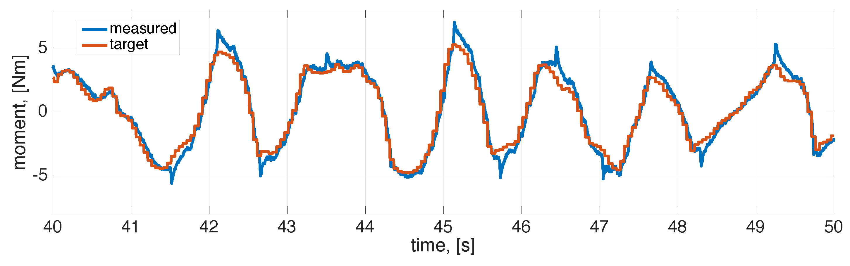
3.3.1. Force Controller Performance

For the PTO simulator to be effective, the measured force must match well with the target force. At a minimum, the PI controller must provide the target force in the frequency band covering the incoming wave spectrum. The Aalborg University Hydraulics Laboratory deep-water wave facility in Aalborg, Denmark, with wave period range 0.7 to 2 s, was used for the experiments.

Figure 9 shows the comparison between target and measured force for an irregular sea state.

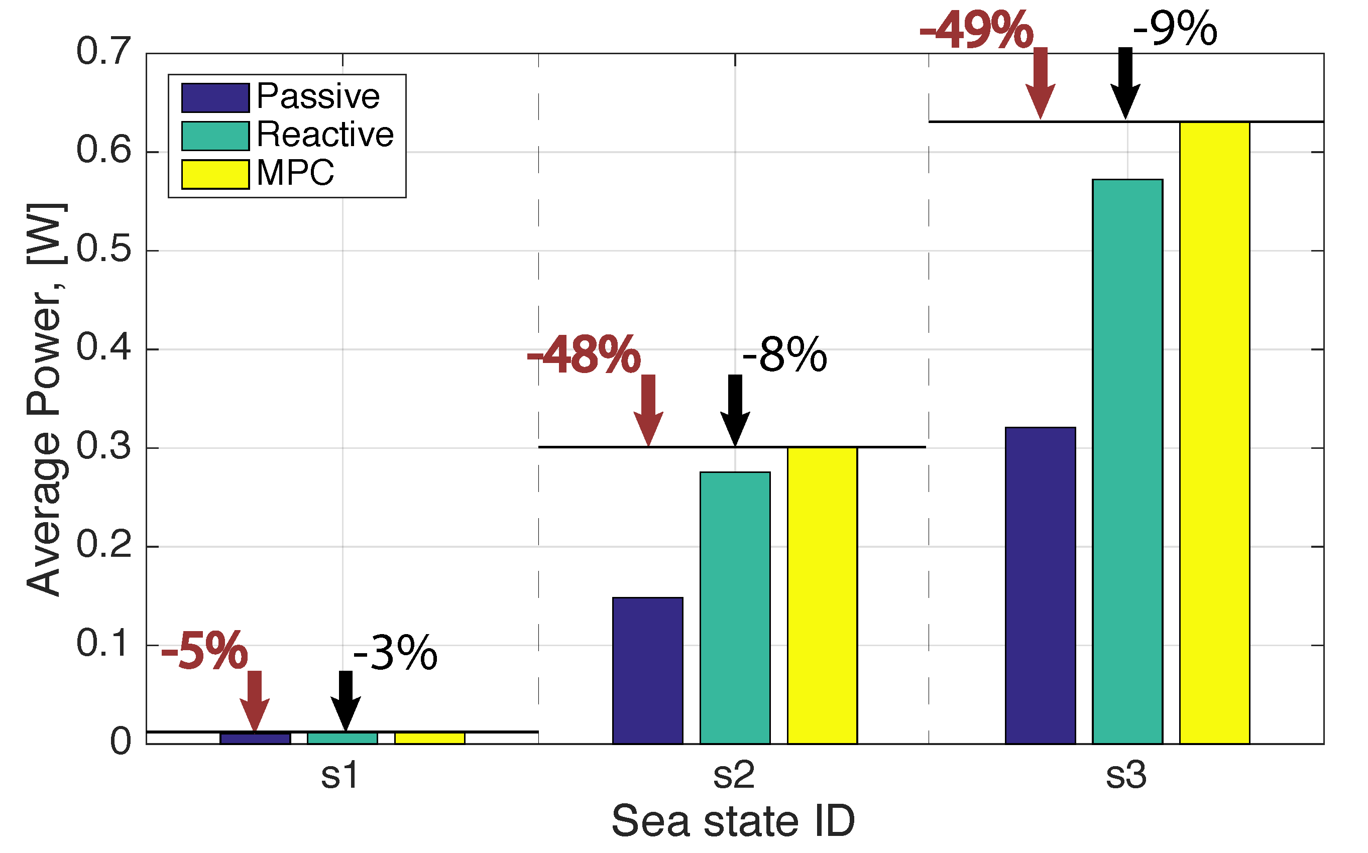
3.3.2. Power Performance

The WEC fitted with MPC has been tested in three different sea states, for which details are given in

Table 2. Sea state characteristics, water depth 0.60 m.

Sea State Name	Spectrum Type	T${}_{\mathit{p}}$ [s]	H${}_{\mathit{m}0}$ [m]	Sample Time [s]
s1	JONSWAP, $gamma=3.3$	$0.9$	$0.045$	270
s2	JONSWAP, $gamma=3.3$	$1.2$	$0.045$	360
s3	JONSWAP, $gamma=3.3$	$1.5$	$0.045$	450

. The sea states are generated using the Aalborg University Civil Dept. in house software AwaSys6 [30] with a white noise method [30]. To quantify the performance of the MPC controller, the WEC was tested with two alternative PTO configurations in identical sea states.

The first alternative is referred to as “passive controller”. It uses a PTO feedback control architecture based on Equation (2), where $m_{pto}=k_{pto}=0$, i.e., only the damping term, $c_{pto}$ is applied. The PTO damping coefficient is chosen based on a numerical look up table and held fixed over the full sea state.

The second PTO alternative, referred to as the “reactive controller,” also uses a PTO feedback control architecture based on Equation (2) but where $k_{pto}\ne 0$, i.e., the stiffness $k_{pto}$ and damping term $c_{pto}$ are both used. The PTO damping and stiffness coefficients are chosen based on a numerical look up table and held fixed over the full sea state.

The difference between the reactive and passive controllers is: the reactive controller provides mechanical power back to the floater during a fraction of the wave cycle in order to increase the band-width of the system response, thus increasing the overall power production [31]; however, it uses no predictive capacity. The MPC is also a reactive controller, but due to its optimization of the PTO force in real time using prediction of the future motion, it is expected to outperform the non-predictive reactive controller.

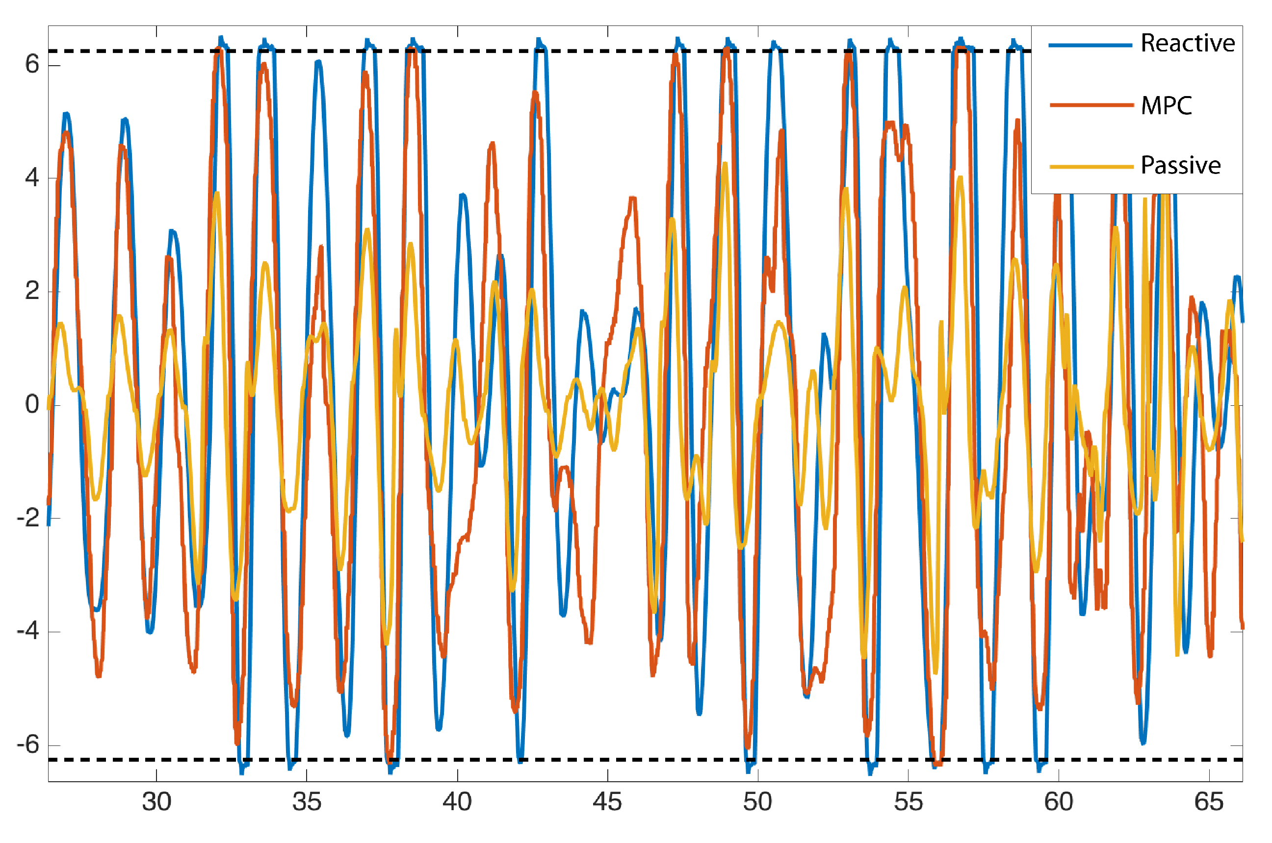
Figure 10 shows the power performance of the three controllers for the three sea states analyzed.

Figure 11 shows a comparison of measured PTO moment for the MPC (red line) with the passive (yellow line) and reactive (blue line) controllers. The black dashed line indicates the PTO moment limit of 6.25 Nm. The amplitude of the control signal for the MPC and reactive controllers are in the same range, while the passive controller requires less effort from the PTO. The timeseries variance is, respectively, 11.37, 10.1 and 2.33 Nm${}^2$ for the Reactive, MPC and Passive controllers.

3.4. Discussion

For the single float Wavestar WEC, the LinMot built-in PI force controller provides a reasonably successful force tracking performance as shown in Figure 9. The figure shows a small phase error and good agreement in terms of amplitude. The spikes visible in the measured force signal are because the PI controller is unable to react to the system friction. Figure 10 shows that the active and MPC controllers perform better than the passive PTO controller by an average factor two, for the sea states where most of the incoming energy is placed at frequencies that are far from the floater heave resonant frequency. Since sea state s1 is close to the natural resonance condition of the WEC, the passive controller performs nearly as well as the other controllers. The comparison between the reactive and the MPC controllers reveals that the prediction of the future state of the system improves the WEC power production.

Furthermore, observing the force output timeseries in Figure 11, although the reactive and MPC controllers have roughly the equivalent wave energy absorption performance, the PTO with reactive controller often hits the maximum PTO moment limit. When the limit is reached, the controller must apply a brake to the PTO connection, thus dissipating useful energy. From this observation, we find that a critical difference between MPC and the reactive controller is the MPC controller’s ability to foresee and prevent situations where the floater must be decelerated due to reaching the maximum PTO moment limit.

4. Conclusions

The versatility of actively controlled PTO simulators has been demonstrated by presenting two successful implementations in experimental WEC models.

In the first application, the PTO simulator was used to implement an idealized passive damping control on a two-body point absorber in regular waves. The PTO simulator allowed the researchers to specify the PTO impedance directly in the experiment. As a result, the PTO simulator approach facilitated rigorous characterization of the two-body point absorber’s performance as a function of wave frequency. Identified drawbacks of that particular implementation are (a) the sensitivity of the system to sensor noise when the PTO force is necessarily large at wave frequencies near the resonance condition/peak performance of the WEC and (b) to ensure controller stability, as evidenced by stability analysis, there is a need to re-tune the feedback controller’s PI coefficients for each combination of PTO coefficients under test. However, the recommendations for improving the method may indeed alleviate these concerns.

In the second application, the PTO simulator architecture allowed for a model-predictive control to be successfully applied to a single-body point absorber in irregular waves. The method enabled a successful assessment of MPC methods in comparison to alternative control strategies, resulting in a quantification of the advantages of an optimal reactive control made possible by the MPC technique over passive control methods.

In general, both applications of the PTO simulator method resulted in the desired research outcomes. Although there are additional complexities and costs to the PTO simulation method, the functional benefits and flexibility of actively controlled PTO simulators for assessing WEC concepts and control systems at physical model scale are very high. It is the authors’ hope that research groups can make use of the presented methods to advance and improve their experimental wave energy conversion research.

References

- Payne, G.S.; Taylor, J.R.; Ingram, D. Best practice guidelines for tank testing of wave energy converters. J. Ocean Technol. 2009, 4, 39–69. [Google Scholar]
- Flocard, F.; Finnigan, T. Experimental Investigation of Power Capture from Pitching Point absorbers. Available online: http://www.homepages.ed.ac.uk/shs/Wave%20Energy/EWTEC%202009/EWTEC%202009%20%28D%29/papers/251.pdf (accessed on 7 July 2017).
- Bailey, H.; Bryden, I. The Influence of a Mono-Directional PTO on a Self-Contained Inertial WEC. Available online: http://www.homepages.ed.ac.uk/shs/Wave%20Energy/EWTEC%202009/EWTEC%202009%20%28D%29/papers/250.pdf (accessed on 7 July 2017).
- Pecher, A.; Kofoed, J.; Espedal, J.; Hagberg, S. Results of an experimental study of the langlee wave energy converter. In Proceedings of the Twentieth International Offshore and Polar Engineering Conference, Beijing, China, 20–25 June 2010; Volume 1, pp. 877–885. [Google Scholar]
- Taylor, J.R.M.; Mackay, I. The Design of an Eddy Current Dynamometer for a Free-Floating Sloped IPS Buoy. Available online: http://www.homepages.ed.ac.uk/v1ewaveg/sloped%20IPS/The%20Design%20of%20an%20eddy%20current%20etc%20etc.pdf (accessed on 7 July 2017).
- Lopes, M.F.P.; Henriques, J.C.C.; Lopes, M.C.; Gato, L.M.C.; Dente, A. Design of a Non-Linear Power Take-Off Simulator for Model Testing of Rotating Wave Energy Devices. Available online: http://www.homepages.ed.ac.uk/shs/Wave%20Energy/EWTEC%202009/EWTEC%202009%20%28D%29/papers/183.pdf (accessed on 7 July 2017).
- Villegas, C.; van der Schaaf, H. Implementation of a pitch stability control for a wave energy converter. In Proceedings of the Ninth European Wave and Tidal Conference, Southampton, UK, 5–9 Sepember 2011. [Google Scholar]
- Zurkinden, A.; Ferri, F.; Beatty, S.; Kofoed, J.; Kramer, M. Non-linear numerical modeling and experimental testing of a point absorber wave energy converter. Ocean Eng. 2014, 78, 11–21. [Google Scholar] [CrossRef]
- Beatty, S.J. Self-Reacting Point Absorber Wave Energy Converters. Ph.D. Thesis, University of Victoria, Victoria, BC, Canada, 2015. [Google Scholar]
- Cummins, W. The impulse response function and ship motions. Schiffstechnik 1962, 47, 101–109. [Google Scholar]
- Clauss, G.; Lehmann, E.; Ostergaard, C. Offshore Structures; Springer Science & Business Media: Berlin, Germany, 2012. [Google Scholar]
- Falnes, J. Wave-energy conversion through relative motion between two single-mode oscillating bodies. J. Offshore Mechan. Arct. Eng. 1999, 121, 32–38. [Google Scholar] [CrossRef]
- Zare, M.; Marzband, M. Calculation of Cogging Force in Permanent Magnet Linear Motor Using Analytical and Finite Element Methods. Available online: http://mjee.org/index/index.php/ee/article/view/310/pdf (accessed on 7 July 2017).
- Duarte, T.; Alves, M.; Jonkman, J.; Sarmento, A. State-Space Realization of the Wave-Radiation Force within FAST. Available online: http://www.nrel.gov/docs/fy13osti/58099.pdf (accessed on 7 July 2017).
- Version 8.2.0.701 (R2013b), The MathWorks Inc.: Natick, MA, USA, 2013.
- Chen, T.; Francis, B.A. Optimal Sampled-Data Control Systems; Springer Science & Business Media: Berlin, Germany, 2012. [Google Scholar]
- Beatty, S.J.; Hall, M.; Buckham, B.J.; Wild, P.; Bocking, B. Experimental and numerical comparisons of self-reacting point absorber wave energy converters in regular waves. Ocean Eng. 2015, 104, 370–386. [Google Scholar] [CrossRef]
- Wavestar. 2016. Available online: http://wavestarenergy.com/concept (accessed on 27 January 2016).
- Yu, Z.; Falnes, J. State-space modelling of a vertical cylinder in heave. Appl. Ocean Res. 1995, 17, 265–275. [Google Scholar] [CrossRef]
- Tona, P.; Nguyen, H.; Sabiron, G.; Creff, Y. An Efficiency-Aware Model Predictive Control Strategy for a Heaving Buoy Wave Energy Converter. Available online: https://hal-ifp.archives-ouvertes.fr/hal-01443855/document (accessed on 7 July 2017).
- Fossen, T.I. Handbook of Marine Craft Hydrodynamics and Motion Control; John Wiley & Sons: Hoboken, NJ, USA, 2011. [Google Scholar]
- Ferri, F.; Ambühl, S.; Kofoed, J.P. Influence of the Excitation Force Estimator Methodology within a Predictive Controller Framework on the Overall Cost of Energy Minimisation of a Wave Energy Converter. Available online: http://vbn.aau.dk/ws/files/224093895/Influenceoftheexcitationforceestimatormethodologywithinapredictivecontrollerframeworkontheoverallcostofenergyminimisationofawaveenergyconverter.pdf (accessed on 7 July 2017).
- Fusco, F.; Ringwood, J.V. Short-term wave forecasting for real-time control of wave energy converters. IEEE Trans. Sustain. Energy 2010, 1, 99–106. [Google Scholar] [CrossRef]
- Brekken, T.K. On model predictive control for a point absorber wave energy converter. In Proceedings of the 2011 IEEE Trondheim PowerTech, Trondheim, Norway, 19–23 June 2011; pp. 1–8. [Google Scholar]
- Gieske, P. Model Predictive Control of a Wave Energy Converter: Archimedes Wave Swing. Ph.D. Thesis, Delft University of Technology, Delft, The Netherlands, 2007. [Google Scholar]
- Fischer, B.; Kracht, P.; Perez-Becker, S. Online-algorithm using adaptive filters for short-term wave prediction and its implementation. In Proceedings of the 4th International Conference on Ocean Energy (ICOE), Dublin, Ireland, 17–19 October 2012. [Google Scholar]
- Hals, J.; Falnes, J.; Moan, T. Constrained optimal control of a heaving buoy wave-energy converter. J. Offshore Mechan. Arct. Eng. 2011, 133, 1–15. [Google Scholar] [CrossRef]
- Cretel, J.A.; Lightbody, G.; Thomas, G.P.; Lewis, A.W. Maximisation of energy capture by a wave-energy point absorber using model predictive control. IFAC Proc. Vol. 2011, 44, 3714–3721. [Google Scholar] [CrossRef]
- Li, G.; Belmont, M.R. Model predictive control of a sea wave energy converter: A convex approach. IFAC Proc. Vol. 2014, 47, 11987–11992. [Google Scholar] [CrossRef]
- “Awasys”. 2016. Available online: http://www.hydrosoft.civil.aau.dk/awasys/ (accessed on 7 July 2017).
- Falnes, J. Ocean Waves and Oscillating Systems: Linear Interactions Including Wave-Energy Extraction; Cambridge University Press: Cambridge, UK, 2002. [Google Scholar]
Figure 1.
1:25 scale two-body point absorber WEC with PTO simulator components.
Figure 2.
System diagram for the original PTO simulator.
Figure 3.
Simplified representation of the PTO simulator controller.
Figure 4.
Two-body point absorber (a) optimal and experimentally applied (b) displacement amplitudes; and (c) mechanical power in regular waves.
Figure 5.
PTO force time series in regular waves of frequency (a) rad/s (b) rad/s. The “commanded” and “measured” signals are the reference force and the measured force output of the PTO, respectively. Plots (c) and (d) are the error time series between the measured and commanded force signals, normalized by the maximum of the commanded force time series; (e) variance of the PTO Force Noise as a function of frequency for 4 cm and 6 cm wave heights. is post-processed through a 124th order, low pass filter with 8 rad/s cut-off.
Figure 6.
Zeros (O) and poles (X) of the closed loop transfer function (Figure 3) for different values of (a) , (b) , (c) , and (d) .
Figure 7.
1:20 physical model of a Wavestar single floater with annexed instrumentation.
Figure 8.
Block-diagram of the complete numerical model and detailed description of the controller block.
Figure 9.
Comparison between target and measured moments on the model scale Wavestar WEC.
Figure 10.
Power performance as a function of the sea state for a passive controller, reactive controller and the MPC.
Figure 11.
Measured PTO moment [Nm] as a function of time [s] from the wavestar point absorber physical model operating with passive, reactive, model-predictive controllers in sea state s3.