Using Thermostats for Indoor Climate Control in Office Buildings: The Effect on Thermal Comfort
by
 ,
,
Georgios D. Kontes
1,2,* ,
,
Georgios I. Giannakis
3,
Philip Horn
4,
Simone Steiger
2 and
Dimitrios V. Rovas
5 1
Department of Mechanical Engineering and Building Services Engineering, Technische Hochschule Nürnberg Georg Simon Ohm, 90489 Nuremberg, Germany
2
Technical Building Systems Group, Nuremberg Branch, Department of Energy Efficiency and Indoor Climate, Fraunhofer Institute for Building Physics, 90429 Nuremberg, Germany
3
School of Production Engineering and Management, Technical University of Crete, Chania 73100, Greece
4
Energy Department, Austrian Institute of Technology, 1220 Vienna, Austria
5
The Bartlett School of Environment, Energy and Resources, Faculty of the Built Environment, University College London, London WC1E 6BT, UK
*
Author to whom correspondence should be addressed.
Energies 2017, 10(9), 1368; https://doi.org/10.3390/en10091368
Submission received: 23 May 2017
/
Revised: 4 September 2017
/
Accepted: 6 September 2017
/
Published: 10 September 2017
Abstract
:Thermostats are widely used in temperature regulation of indoor spaces and have a direct impact on energy use and occupant thermal comfort. Existing guidelines make recommendations for properly selecting set points to reduce energy use, but there is little or no information regarding the actual achieved thermal comfort of the occupants. While dry-bulb air temperature measured at the thermostat location is sometimes a good proxy, there is less understanding of whether thermal comfort targets are actually met. In this direction, we have defined an experimental simulation protocol involving two office buildings; the buildings have contrasting geometrical and construction characteristics, as well as different building services systems for meeting heating and cooling demands. A parametric analysis is performed for combinations of controlled variables and boundary conditions. In all cases, occupant thermal comfort is estimated using the Fanger index, as defined in ISO 7730. The results of the parametric study suggest that simple bounds on the dry-bulb air temperature are not sufficient to ensure comfort, and in many cases, more detailed considerations taking into account building characteristics, as well as the types of building heating and cooling services are required. The implication is that the calculation or estimation of detailed comfort indices, or even the use of personalised comfort models, is key towards a more human-centric approach to building design and operation.
1. Introduction
In modern buildings, it is very common that Building Automation and Control Systems (BACS) are used to ensure parsimonious energy use and cost-effective building operation. This often happens by tuning BACS parameters (e.g., set points) to exploit the inherent trade-off between energy consumption and thermal comfort, with the latter acting as a constraint defining a theoretical and practical upper bound on potential energy savings [1,2,3,4]. Estimation of thermal comfort is a challenging task given the subjectivity of human perception; this subjectivity is reflected in the statistical nature of comfort models, as well as the plethora of comfort models available. It is conceivable that different ways of estimating thermal comfort will alter the operational constraints [5,6] and can influence design and operational decisions. Over-relaxing comfort, while positive from an energetic perspective, can lead to dissatisfied users and incur indirect costs related to productivity loss [7,8].
Estimation of thermal sensation has been the subject of active research for many years, and the knowledge acquired has been incorporated into national and international standards [9,10,11]. Research on building energy management systems and model-based control [12,13,14,15,16,17] hints at the need for proper comfort estimation; a similar view is shared by the industry [18]. Nevertheless, the use of thermostats for temperature regulation remains the current state of practice in most buildings. The thermostats ensure that temperature is maintained within a band around a target set point (e.g., 22 °C ± 2 °C), with the implicit assumption being that within that range, comfort is guaranteed. In practice, this happens mainly due to increased capital and commissioning costs, since calculating complex thermal sensation indices usually requires the installation of additional sensors.
Changing the set point or increasing the dead band can lead to significant energy savings [4,19,20,21,22], but i is also evident from field experiments in spaces with dry-bulb temperature control that users tend to act upon the controllable elements of a building—such as windows, blinds, lights and thermostats—in response to their feeling of thermal discomfort, with potentially detrimental effects to energy performance [23,24,25]. A significant effort has been undertaken within the IEA-EBC Annex 66 project [26], towards analysing and modelling occupant behaviour in buildings, as well as quantifying the impact of users’ behaviour in actual energy consumption.
A review of the findings of Annex 66 can be found in [27]. There, the DNAS (Drivers, Needs, Actions, Systems) framework is presented, capturing four key aspects in the human-building environment interaction:
- Drivers: a set of drivers (or events or triggers) comprises the stimulating factors (such as indoor and outdoor conditions, day of the week, building properties, etc.) that provoke energy-influencing occupant behaviour;
- Needs: needs are the requirements of the occupants that need to be met in order to ensure satisfaction with their environment (e.g., thermal and visual comfort);
- Actions: actions are interactions of occupants with their environment and controllable systems, as well as activities (e.g., changing clothes, drinking water, etc.) that occupants undertake to satisfy their needs;
- Systems: this is the set of controllable building elements (e.g., windows, blinds, thermostats, etc.) available to the user to interact with and restore/maintain comfort.
In agreement with the DNAS framework, stochastic models [28] predicting the probability of an occupant control action can be defined and trained using available field data [29,30,31,32], while a different set of models is used to predict the comfort sensation of occupants in individual spaces and adapt building control to an individual’s needs [28,33,34,35].
The work presented here is intricately linked with the user modelling framework described above. More specifically, we investigate one of the main (and rather overlooked) drivers that trigger user actions in buildings, that of oversimplification in the estimation of user comfort. Zone dry-bulb air temperature measurements when used in isolation might not always by suggestive of the actual thermal sensation of the occupants due to all other factors also affecting thermal comfort in building spaces, such as the effect of solar radiation or humidity [9]. In view of this, the effect of solar radiation on thermal comfort has been studied extensively [36,37], while in [38,39,40,41], controllers able to compensate this effect in buildings with Thermally-Activated Building Systems (TABS) were presented. In this paper, we take a wider view on the effect of dominant parameters affecting thermal sensation and suggest that depending on the thermal characteristics of each building, as well as the types of heating and cooling systems, some of these additional factors should be taken into account.
In our study, two buildings have been selected with contrasting thermal and construction characteristics and different systems to meet heating and cooling demands. The buildings were chosen to highlight differences obtained by the use of widely-available room controllers to ensure indoor comfort conditions. In each case, a systematic exploration of the effect of relevant controller parameters and associated boundary conditions has been performed. The resulting thermal comfort levels are evaluated using Fanger’s thermal comfort index [42]. To ensure the same boundary conditions in all of the experiments and to avoid disturbances from uncontrollable influencing factors, such as occupant’s actions or inaccurate sensor measurements, simulation-based experiments were performed. The findings of the present work support our hypothesis and provide valuable insights, on thermal comfort inefficiencies due to improper regulation, and translate to conclusions that apply in real buildings.
2. Thermal Comfort Evaluation in Buildings
A wide range of methodologies for indoor thermal comfort estimation exist: from simple dry-bulb temperature-tracking [2,43] to more elaborate indices [42,44,45]. The most widely-accepted models, as evidenced by their adoption in indoor climate thermal comfort standards, are: (i) Fanger’s Predictive Mean Vote (PMV) model [42] used in the International Organization for Standardization (ISO 7730) [9] and the American Society of Heating, Refrigerating and Air-Conditioning Engineers (ASHRAE 55) [11] standards; (ii) the Adaptive Comfort Model of the ASHRAE Standard 55-2010 [11]; and (iii) the Adaptive Comfort Model of the European Standard EN 15251 [10].
These methodologies can be put into two broad categories: (i) human body heat balance approaches [42,44,45]; and (ii) thermal adaptation approaches [10,11]. The first category applies to buildings with mechanical Heating, Ventilation and Air Conditioning (HVAC) systems where the building occupants are allowed to control the internal environment to desired levels of air temperature, while the second category applies to naturally-ventilated buildings.
Fanger’s Predicted Mean Vote Model
Fanger’s Predicted Mean Vote (PMV) model is based on human body heat-balance considerations. Taking into account that thermal sensation is influenced by environmental (air temperature, radiant temperature, humidity and air velocity) and personal factors (activity and clothing), the PMV index predicts the thermal comfort on a seven-point sensation scale (−3 cold, −2 cool, −1 slightly cool, 0 neutral, +1 slightly warm, +2 warm and +3 hot). The Fanger Predicted Percentage of Dissatisfied (PPD) people index, derived from the PMV index, predicts the percentage of a large group of people likely to be thermally (dis-)satisfied with their environment.
Precise quantification of personal factors is a challenging task, due to the difficulty associated with making robust measurements. Instead, metabolic rate estimation methods and predefined clothing insulation values are used. Methods for metabolic rate estimation are divided into four levels in ascending order of accuracy [46]. At Levels 1 (screening) and 2 (observation), look-up tables are used to estimate metabolic rates for various occupation and activity types. At Level 3 (analysis), the metabolic rate is estimated using an empirical correlation to the total heart rate. The total heart rate is the sum of the heart rate at rest and its increase under specified conditions. When the total heart rate is known, a linear relationship can be established between the two parameters. At Level 4 (expertise), the metabolic rate is determined by measuring oxygen consumption and carbon dioxide production rates. Level 3 and 4 methods require measurements that might be hard to collect, and the improvement in accuracy (±20% error for Level 2 vs. ±5% error for Level 4) does not significantly impact the results of our study as a simple sensitivity analysis might show.
The role of clothing as an insulating material is captured by the thermal resistance and typically measured in units of clo. In many applications, constant values of 0.5 clo are used during the cooling season and 1.0 clo during the heating season. To account for the fact that humans adjust their clothing based on prevailing conditions, three predictive clothing insulation models are proposed in ASHRAE 55-2013 [47]; in all of these models, the clothing insulation varies as a function of outdoor air temperature measured early in the morning (at 6:00) and the indoor operative temperature.
Concerning environmental factors, air temperature, humidity and air velocity are relatively easy to measure, and low-cost sensors are readily available and installed in many buildings. Radiant temperature measurements are not frequently performed, except in experimental buildings (both buildings in our study are equipped with such sensors). In cases where sensed measurements of radiant temperature are missing, two methods are commonly used to estimate radiant temperature: the space averaged radiant temperature, calculated assuming that the occupant is at the centre of a space; and the angle-factor radiant temperature, calculated based on angle factors between a person’s location and the different surfaces of a space. As can be inferred from the discussion above, the evaluation of the PMV index is not easy, since many of the parameters have to be estimated or require sensing modalities that may not be available. For this reason, both ASHRAE 55 and ISO 7730 introduce simplified calculation methodologies to define acceptable limits for thermal comfort.
In ISO 7730, the simplification is based on an operative temperature of 24.5 °C in summer and 22.0 °C in winter. These recommendations correspond to zero values of the PMV index, under standard assumptions on the metabolic rate (1.2 met, corresponding to sedentary activity), clothing level (0.5 clo in summer and 1 clo in winter), relative humidity (60% in summer and 40% in winter) and air velocity (as in Table 1). Three different comfort categories are introduced in ISO 7730 with varying ranges, corresponding to varying percentages of the PPD index: (i) Category A is recommended for buildings occupied by people with special thermal comfort requirements (e.g., very young children, the elderly); (ii) Category B is suitable for most new buildings and renovations; and (iii) Category C is suitable for existing, less energy-efficient buildings.
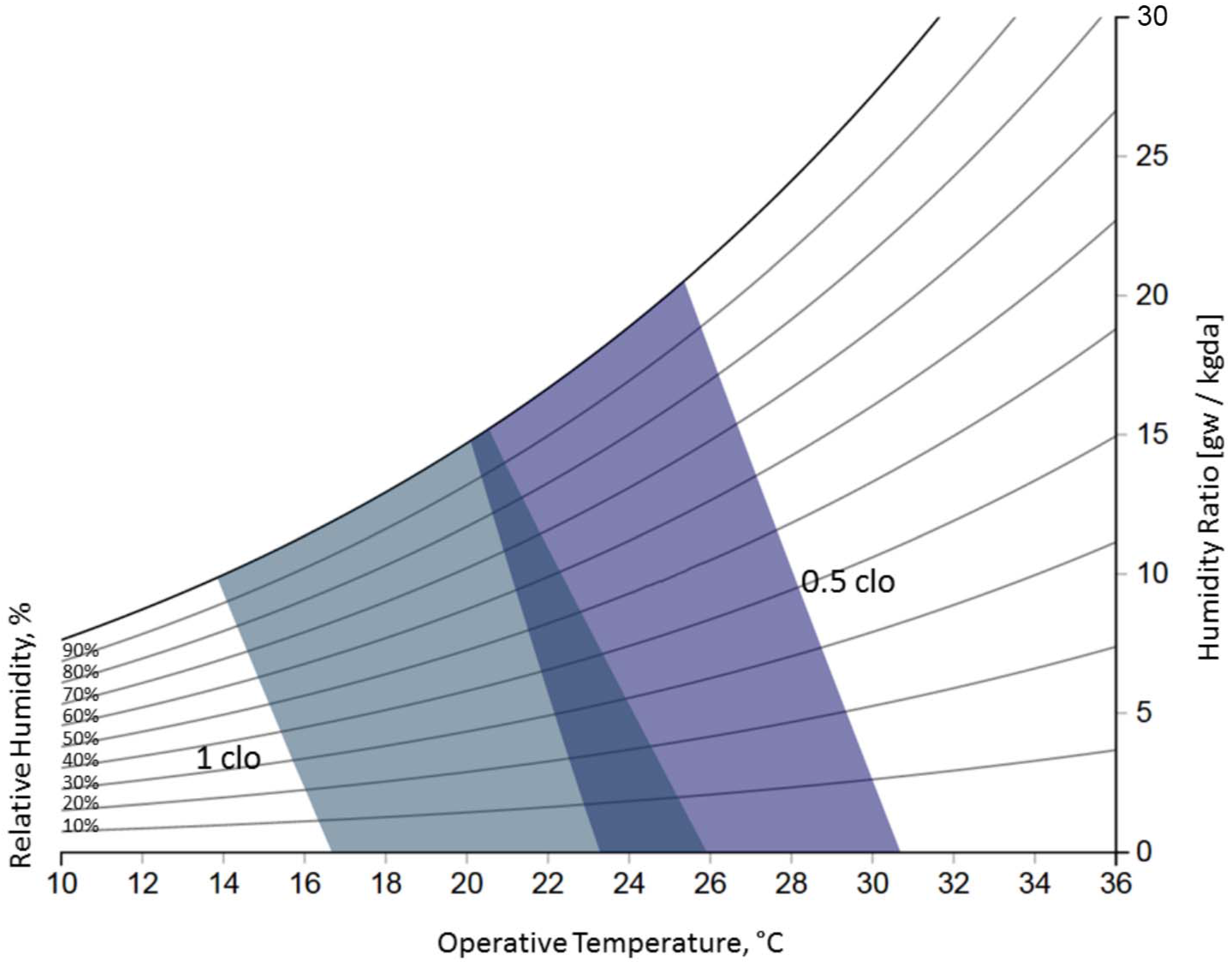
In ASHRAE 55, acceptable ranges of operative temperature (defined as the average of radiant and dry-bulb air temperature) and the humidity ratio are defined. In Figure 1, comfort ranges (shaded polygons) are illustrated for heating season (clothing value = 1.0 clo) and cooling season (clothing value = 0.5 clo), for occupants under light activity (1.2 met). The limits for each season are defined for a value of PPD = 10% (corresponding to −0.5 ≤ PMV ≤ 0.5), where 10% of the users are expected to express discomfort with their environment. The discomfort levels approach a PPD = 10% level near the edges of the polygons and approximate a value of PPD = 5% (or PMV = 0) as we move towards the centre of the shaded areas. We can move to the right of the diagram by heating a space, to the left by cooling it, upwards by humidifying a space and downwards by dehumidifying it.
3. Methodology
In current practice, the operative temperature values defined in the ISO 7730 comfort limits (Table 1) are used as reference values for programming room thermostats, with the difference that the measured temperature is usually not the operative temperature, but rather the dry-bulb air temperature. This practice is based on two assumptions: (i) the values of air and operative temperatures in each building space are (more or less) identical; and (ii) maintaining the operative temperature within some predefined bounds throughout occupied periods suffices to ensure thermal comfort for the occupants, since usually, still-air internal environments with moderate humidity levels are assumed.
Both of these assumptions are not without issues. First, the assumption that air temperature can be a proxy for operative temperature is true only if the radiant temperature that is linked to building surfaces temperatures is not too different. This is very frequently the case in buildings with TABS systems; in this case, local discomfort can be minimized and an almost uniform vertical temperature distribution can be achieved that matches the ideal comfort temperature profile. Even in this case, solar and internal gains can lead to discrepancies between radiant and air temperature. Second, the assumption of pre-defined and static bounds for the operative temperature alone suggests that this is the dominant factor, but neglecting other personal (clo value) and environmental (humidity) factors can be pernicious.
The experiments presented in the next section aim at quantifying the divergence from the designed thermal comfort levels for buildings controlled by simple thermostats, developed and applied based on the aforementioned assumptions. For our hypothesis testing, two buildings have been selected with significant differences in terms of construction and building services systems: the Technical Services Building of Technical University of Crete (TUC) building in Chania, Greece; and the “Zentrum für Umweltbewusstes Bauen” (ZUB) office building in Kassel, Germany. The TUC building has a light-weight construction, low levels of insulation and relatively poor air tightness; while arguably not the best building from an energetic or comfort perspective, it can be considered as an archetype of many buildings in South Europe. The ZUB building has a very high thermal mass, exceptional levels of insulation, good airtightness and exemplifies a high-performance low-energy building built to passive house standards.
We have intentionally selected two buildings that represent the two “extrema” of the spectrum regarding their thermal characteristics. This will allow us to quantify the significance of thermal mass in the air/operative temperature mismatch (and in maintaining comfortable interiors in general). Our research findings could be generalized for all of the building types in between.
3.1. Simulation Model of the TUC Building
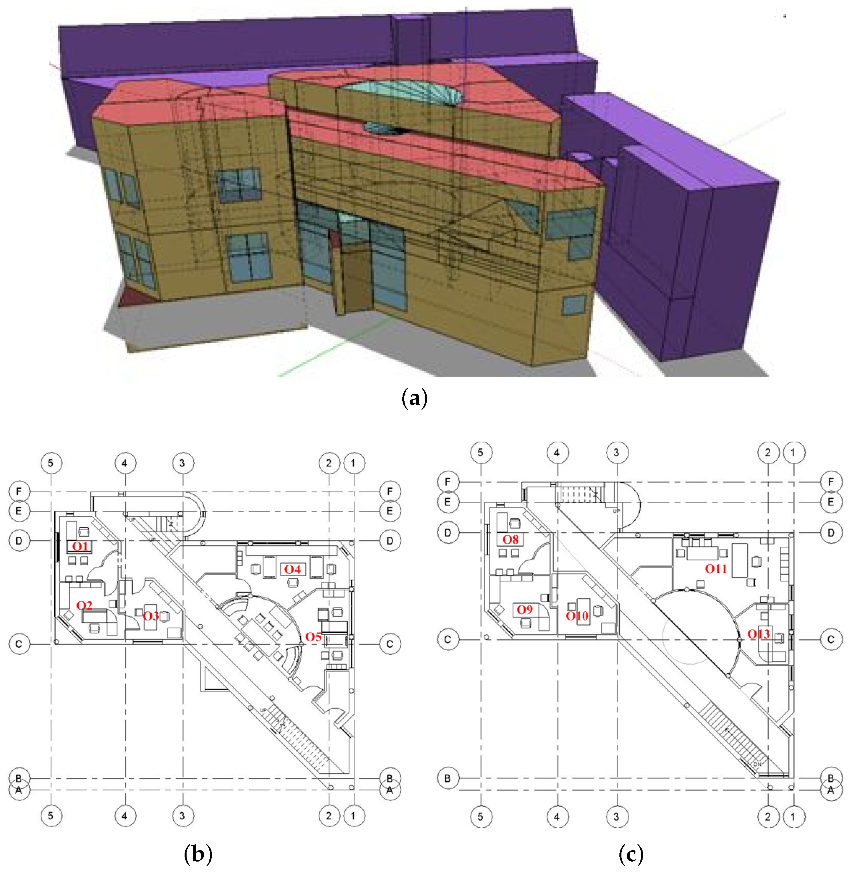
The TUC building is located in a thinly-built-up area on the outskirts of Chania, Greece. The building is a two-storey office building with a basement and a total surface area of 450 m2. It has a north-northwest orientation with large openings and an atrium. The region is characterized by long hot summers, cold humid winters and long periods of sunlight during the year, typical of a Mediterranean climate. A simulation model of the building has been created using EnergyPlus as the simulation engine [49]. A detailed geometric model was created using the floor plans and on-site measurements to capture the as-built condition of the building. To account for shading from nearby buildings, shading surfaces of neighbouring buildings were introduced. Furthermore, based on the building construction data, templates were created for each of the walls (internal partitions, external walls, roof, etc.) detailing thermal characteristics. The OpenStudio plugin (v1.4.2) for SketchUp (Figure 2) was used to generate the first version of the EnergyPlus Input Data File (IDF).
These files were further edited to include systems and other relevant simulation parameters. Heating is achieved through a central system using an oil boiler and hot water radiators in each room, while a Packaged Terminal Heat Pump (PTHP) unit is installed in each office for cooling, with detailed modelling of both systems in EnergyPlus. Heat gains due to infiltration and ventilation can be significant, and as such, a detailed modelling of the infiltration/ventilation was performed using EnergyPlus Airflow Network [50], enabling the multi-zone airflow calculation driven by outdoor wind and forced air (due to HVAC systems’ operation). To correctly account for internal gains due to occupant presence and their thermal sensation, activity data have been collected for the building and imported in the model. The types of data imported include occupant density (people/m2) in each zone, metabolic rates for office activities and occupants’ clothing insulation. Computer and equipment gains have also been introduced for each zone of the building, as well as lighting data (type of lights, energy requirement, visible and radiant fractions).
Towards increasing the indoor relative humidity estimation’s accuracy, the Effective Capacitance (EC) model has been adopted in the thermal simulation model, estimating the moisture absorption into the materials, often neglected by building thermal simulation models [51]; here, a moisture capacitance multiplier equal to 15 was used to combine this term with the zone air [51].
The TUC building is well monitored both for energy use, but also for indoor air parameters, including dry-bulb temperature, humidity and radiant temperature sensors in all rooms. Although our methodology is based on a simulation for the reasons explained above, these data have been used to validate the model and ensure it captures the building performance both from an energetic performance, but also from an indoor thermal comfort perspective. More details on the simulation model details and its validation can be found in [17,52].
3.2. Simulation Model of the ZUB Building
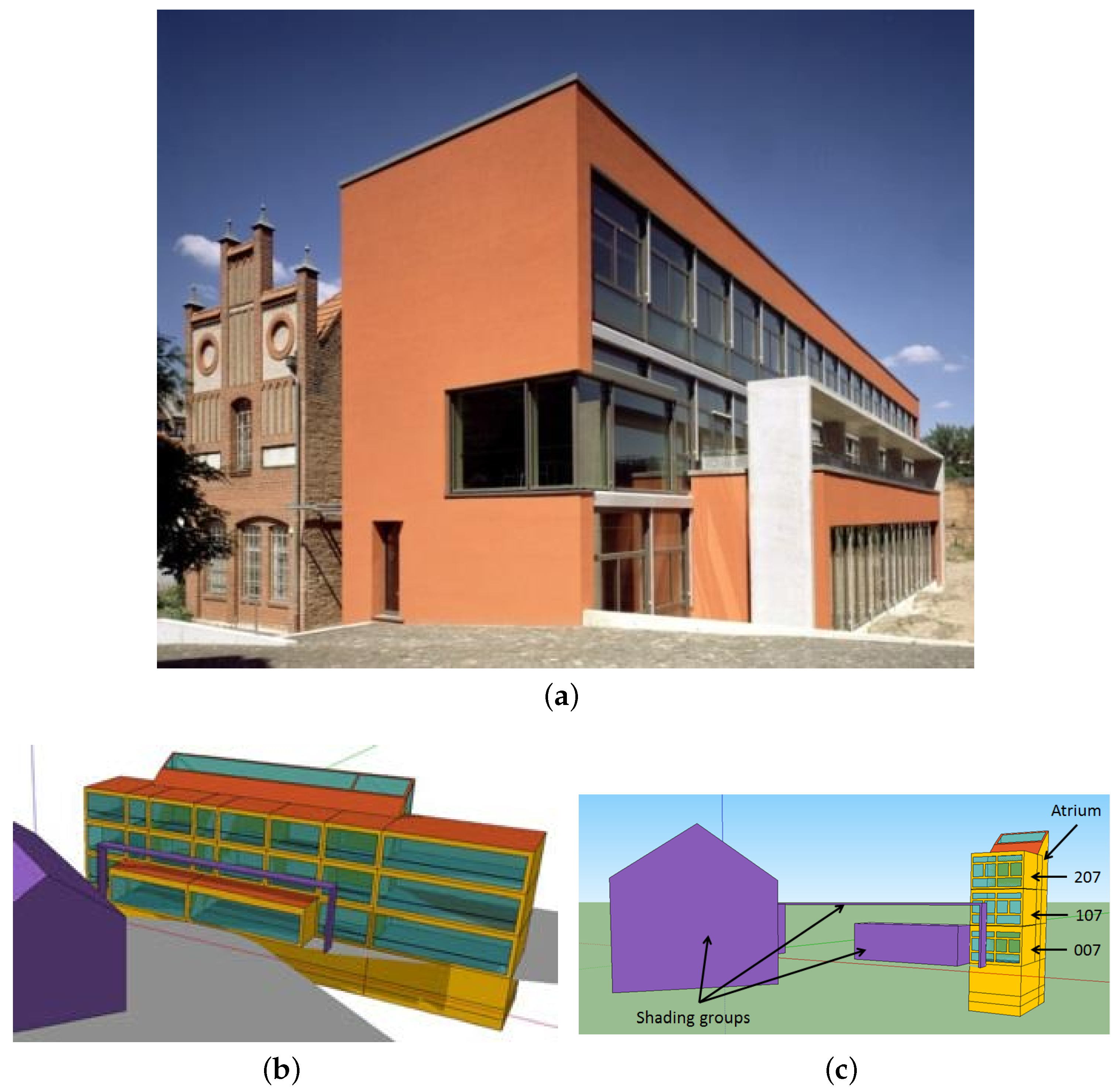
The ZUB building (Figure 3a) is a low-energy office building, characterized by high thermal mass, good airtightness and a south-facing facade with a high (62%) glazing ratio. It is a well-insulated building, with the U-value of the exterior walls equal to 0.11 W/m2K and triple-glazed windows with a U-value of 0.6 W/m2K.
The building is equipped with a radiant surface heating system with heat supplied in each of the office spaces via thermally-activated floors. The building is connected to a district heating network, and the supply water temperature is regulated based on the average outside temperature during the last 24 hours. A mechanical ventilation system with heat recovery has been installed; fresh air is heated and supplied to the office rooms, while exhaust air is extracted from the atrium and passed through the heat recovery unit.
The simulation model of the ZUB building was developed using the TRNSYS 17 [53] whole-building simulation tool. The building exhibits periodicity, and a simplified three-office tower model is able to capture all relevant dynamics as described in more detail in [54] and shown in Figure 3c. The tower model (Figure 3b) consists of three offices (25 m2 each) and an adjacent atrium. Here, the east and west walls of the building are modelled as heavy-weight external walls with a total thickness of 0.5 m and a U-value of 0.113 W/m2K, with the same construction also used for the side walls of the atrium. An identical occupancy schedule is assumed for all 3 offices of the tower model from Monday–Friday. The offices are occupied with 2 persons each from 9:00–12:30 and from 13:15–17:30, while the internal gains are set according to the Verein Deutscher Ingenieure (VDI) 2078 (Class 1 at 23 °C) [55].
It should be noted that the TUC model was developed in EnergyPlus, whereas the ZUB model was developed in TRNSYS. The actual choice of tool is not important and was dictated by specific requirements of a research project; see the Acknowledgements section. Both EnergyPlus and TRNSYS are whole-building simulation tools, and while differences exist in the modelling approach taken, both have been validated under standard validation procedures [56,57]. What is more important is that both buildings, being research buildings, are well instrumented (including radiant temperature sensors); and the sensor data acquired from the available building management system have been used to validate the two models to the same exacting detail. As such, we are confident that these models properly capture the actual buildings’ behaviour and do not introduce unwanted artefacts.
4. Results and Analysis
Summer and winter operation simulation experiments were performed for the TUC building. In each mode, two numerical experiments were performed: one assuming a thermostat that regulates heating or cooling based on dry-bulb air temperature measurements, representing current practices; and one based on operative temperature control. In winter operation, heating is delivered to the spaces using radiators, whereas in summer operation, cooling is delivered by the PTHP units in each office. These experiments provide some insights to the first assumption in Section 3, namely quantifying the impact on thermal comfort when air temperature is used as a proxy. Furthermore, the discussion contributes to the development of some understanding of the effect that different types of systems (radiant or air-based) have on thermal comfort.
In the case of the ZUB building, only winter experiments were performed; in summer, the building is naturally ventilated, and set-point control is not relevant. Heating is delivered using the TABS system, which can be independently controlled in each office; a ventilation system is serving all offices, maintaining acceptable indoor air quality. This allows us to evaluate the effect of internal and solar gains on the comfort conditions in the offices.
For both buildings, the Fanger PPD index is utilized to evaluate the thermal comfort levels, with the values of the Fanger index at each time step of the simulation being a simulation output for both EnergyPlus and TRNSYS simulation engines. Even though according to ISO 7730, both buildings should belong to Class C (see Table 1), as they are existing buildings, the thermal properties of the ZUB building allow reaching Class A comfort levels, at least in the simulation, where the internal gains and occupant behaviour are deterministic. This means that for the experiments below, we define a 15% Fanger PDD limit for the TUC building and a 6% Fanger PPD limit for the ZUB building.
For all of the experiments both in the TUC and ZUB building, we have selected to operate the heating system continuously during night and day. This is due to the simple structure of the controllers applied, which can lead to poor tracking of the temperatures when switching to different comfort bounds during the transition between unoccupied to occupied periods, due to the inability to incorporate weather and occupancy predictions [58].
In the remaining part of this section, the results from all of the experiments for the TUC and ZUB building are illustrated.
4.1. TUC Building
For the summer experiments, the period between 1 July and 16 July was examined, using a Meteonorm weather file [59] for the simulation. This period is characterized by hot days, with the average temperature at 26.9 °C, the minimum temperature at 20.4 °C and the maximum temperature at 35 °C. The blinds and the windows of the building are considered always closed, and the operative/air thermostat temperature set-point (controlling the PTHP units in each office) is set at 24.5 °C for the entire simulation period (day-night), following the mean operative temperature shown in Table 1 for summer.
For the winter experiments, the period between 1 January and 16 January was selected using the same weather file. Here, we have some sunny days, with the average temperature at 11.9 °C, the minimum temperature at 5.6 °C and the maximum temperature at 17 °C. The windows in all offices are considered closed, but the blinds are always open to exploit the solar gains for heating. The operative/air temperature set-point (controlling the radiators in each office) is set at 22 °C for the entire simulation period (day-night), again according to the mean operative temperature provided in ISO 7730 (Table 1) for winter.
The results of Offices 04 and 08 are presented in the ensuing discussion. The two offices selected are representative of the thermal behaviour of other offices in the building: Office 04 is south-facing and receives high solar gains both during summer and winter, while Office 08 is north-facing, is more exposed to wind and receives the least amount of solar gains of all offices.
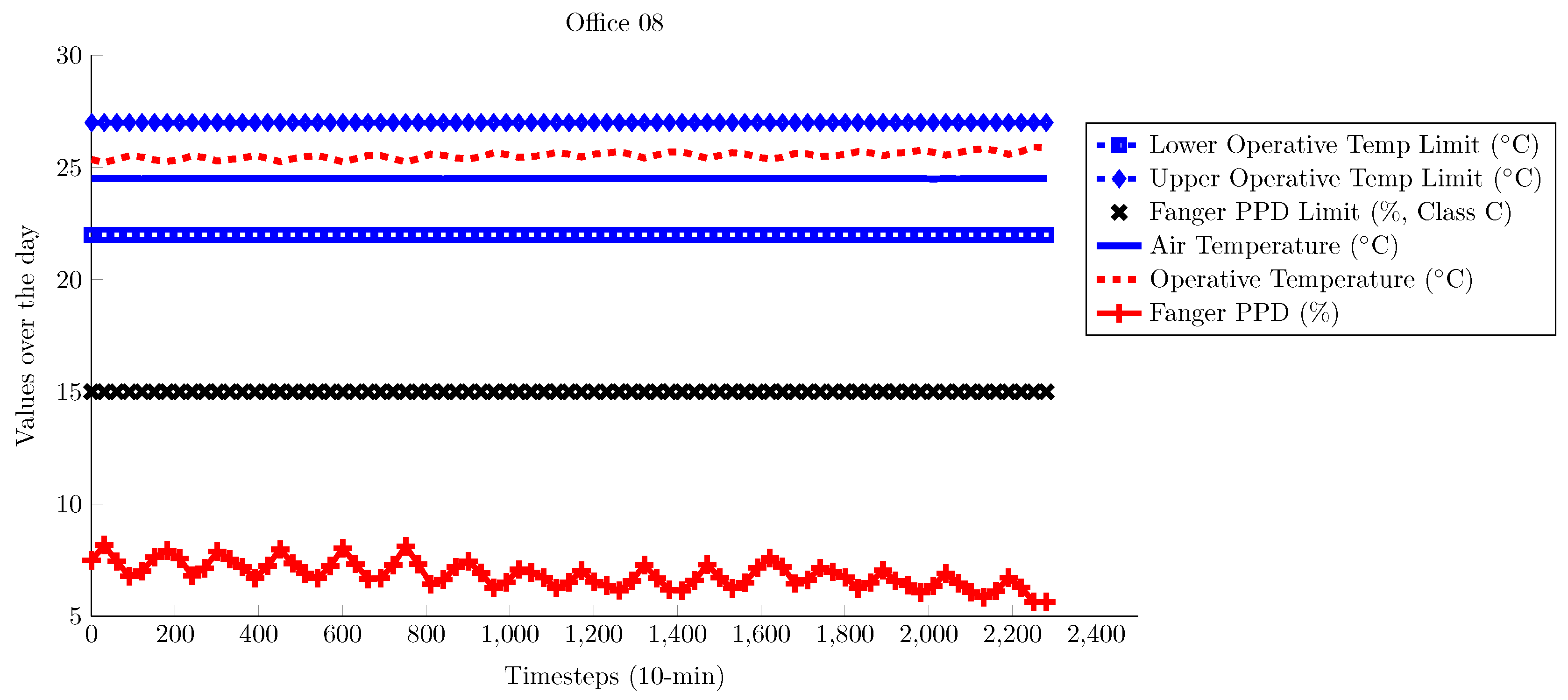
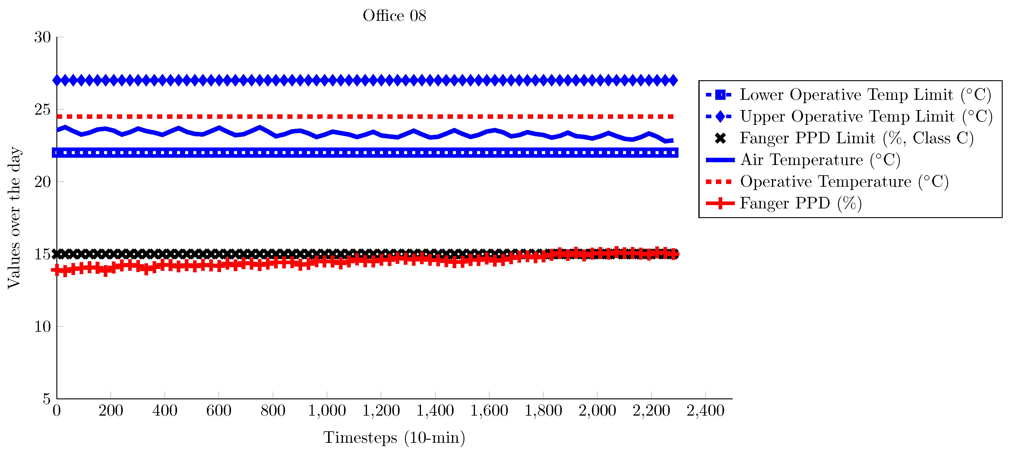
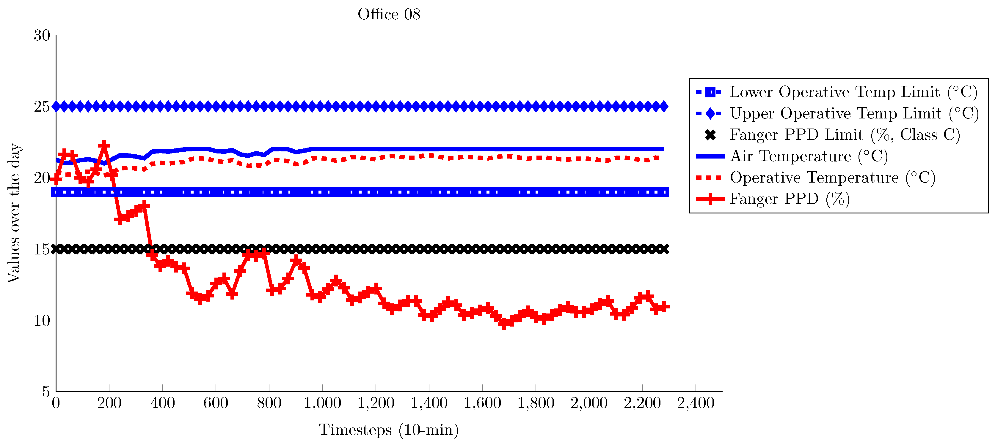
Starting with the summer experiments, Figure 4 illustrates the results for Office 08 using the air temperature thermostat control, where it is obvious that the selected control strategy manages to maintain comfort at acceptable limits, as indicated by the Fanger PPD values. Note that the operative temperature is higher compared to the air temperature, as expected, due to the lightweight construction of the building and the type of HVAC system (air and not radiant system): here, the air system cools the zone air, but the radiant temperature remains higher, leading to higher operative temperatures.
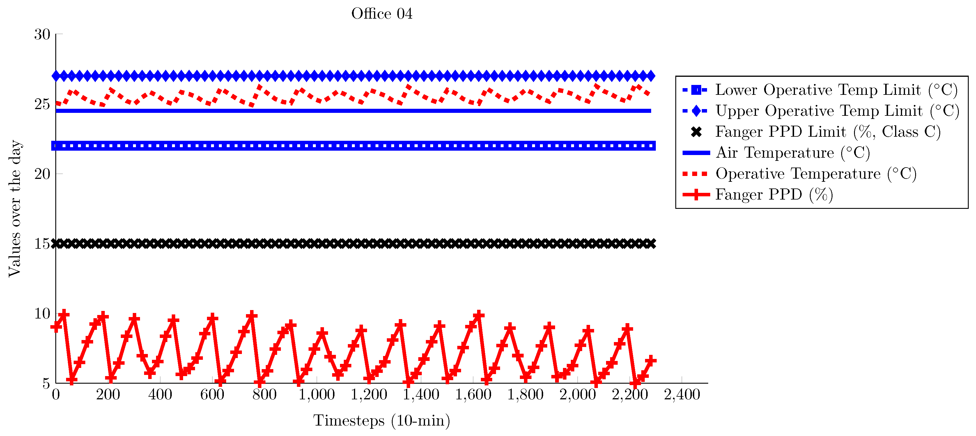
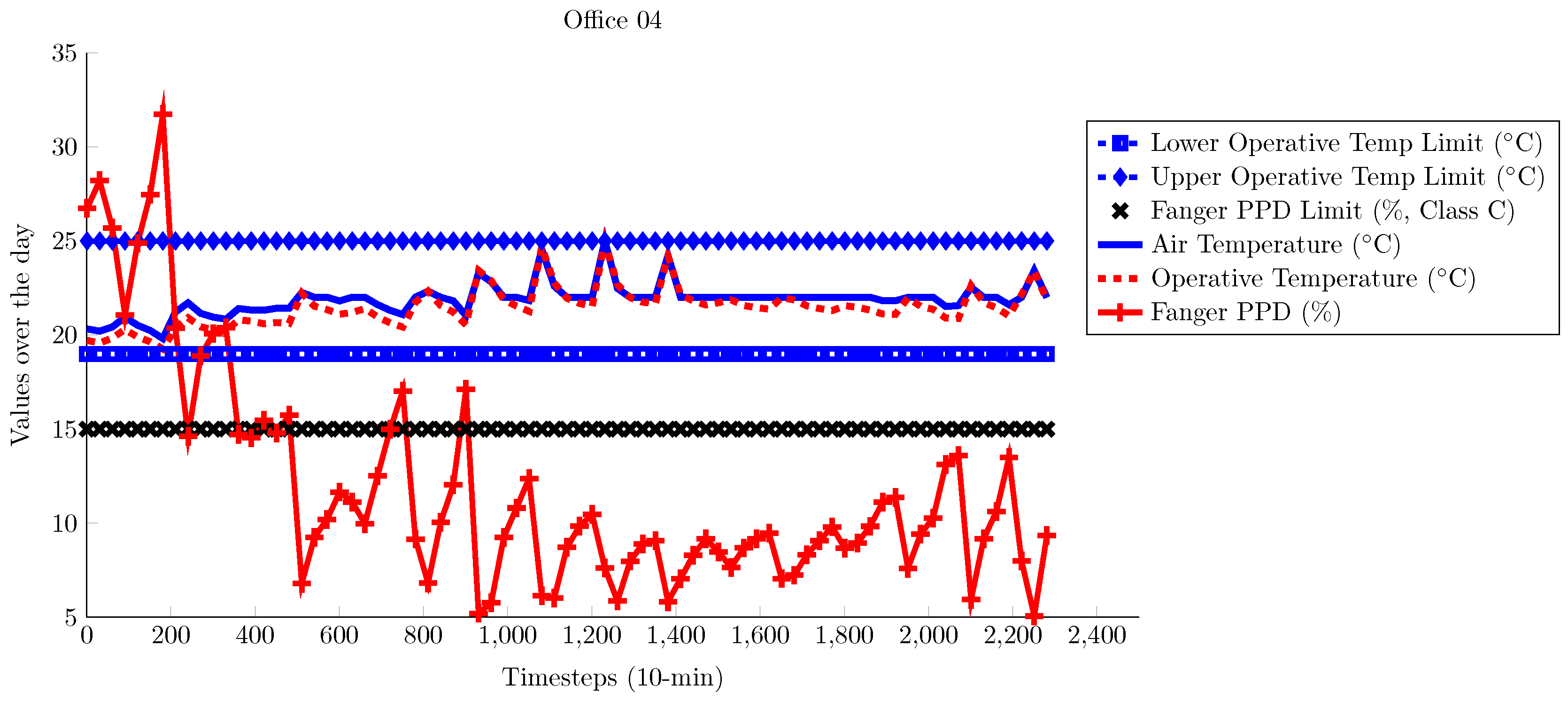
Figure 5 shows the results from the same experiment for Office 04. Similar behaviour with respect to both comfort levels and the incompatibility of air and operative temperatures as with Office 08 is observed, but in this case, the operative temperature values exhibit higher variability, fluctuating between day and night, due to the significantly higher solar gains that Office 04 receives compared to Office 08.
For operative temperature control in the summer experiments, where the thermostat control mode has been modified properly to enable operative, instead of air, temperature control (set-point values refer to the desired operative temperatures), the results for Office 08 are shown in Figure 6. It is obvious that the operative temperature is still higher compared to the air temperature, but also attains lower values compared to the results of the air temperature control shown before (Figure 4). Here, the Fanger PPD values lay on the upper comfort bound due to over-cooling.
Controlling the operative instead of air temperature leads to similar results for Office 04, as well (Figure 7), where the control strategy is characterized by higher discomfort than before (Figure 5), again due to over-cooling.
The fact that even though the operative temperature in both offices is set equal to the design temperature suggested in the ISO 7730 (shown in Table 1), this leads to over-cooling should not come as a surprise. The acceptable temperature and comfort bands in the ISO example tables have been calculated under specific assumptions for all other influencing factors, namely the clo value, metabolic rate and relative humidity levels (constant at 60%). For the experiments presented here, although personal factors are defined according to similar assumptions, the relative humidity levels are not constant, but dynamically calculated by the EnergyPlus simulation engine, resulting to relative humidity values between 40% and 48% approximately for the entire simulation period. These values are substantially lower compared to the relative humidity level assumed in Table 1. Here, higher values of the PPD index are due to the fact that the Fanger comfort model takes into account the heat loss by evaporation of sweat from the human body’s skin; due to sweating effects, when the relative humidity gets higher, occupant thermal sensation is expected to be hotter than the actual temperature.
Towards further investigating the impact of relative humidity on the desired operative temperature for thermal comfort, we use the psychometric chart of Figure 1 as a guideline. Here, taking into account the shaded polygon corresponding to the cooling season (clo = 0.5), we can see that for lower relative humidity values, operative temperature values higher than 24.5 °C are required in order to move closer to the centre of the polygon. Thus, we perform another experiment using 25.5 °C as the set-point to the operative temperature thermostat. Results shown in Figure 8 and Figure 9 highlight the better comfort levels for both offices, a fact that indicates that taking into account the humidity levels in a building when designing the respective operative temperature comfort bounds is crucial for capturing the actual thermal comfort profile of the specific building.
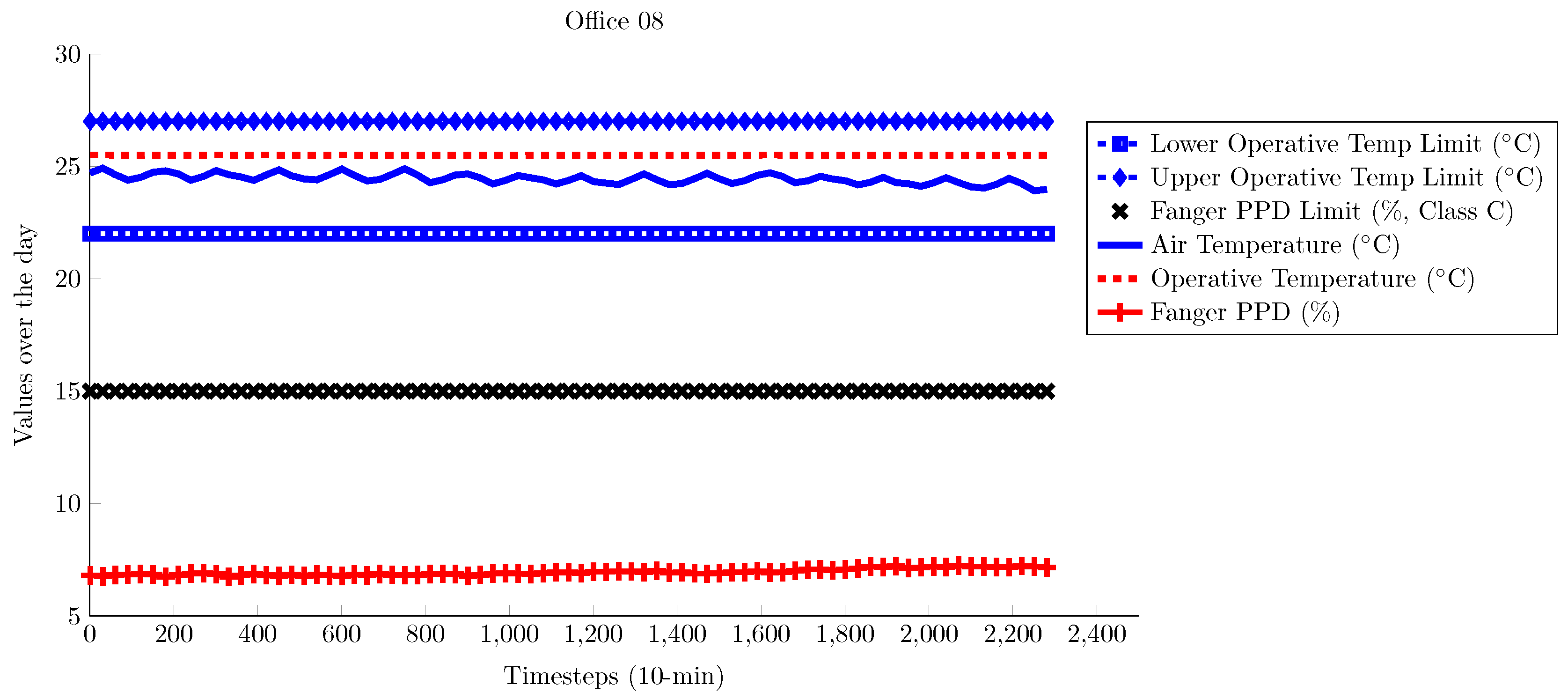
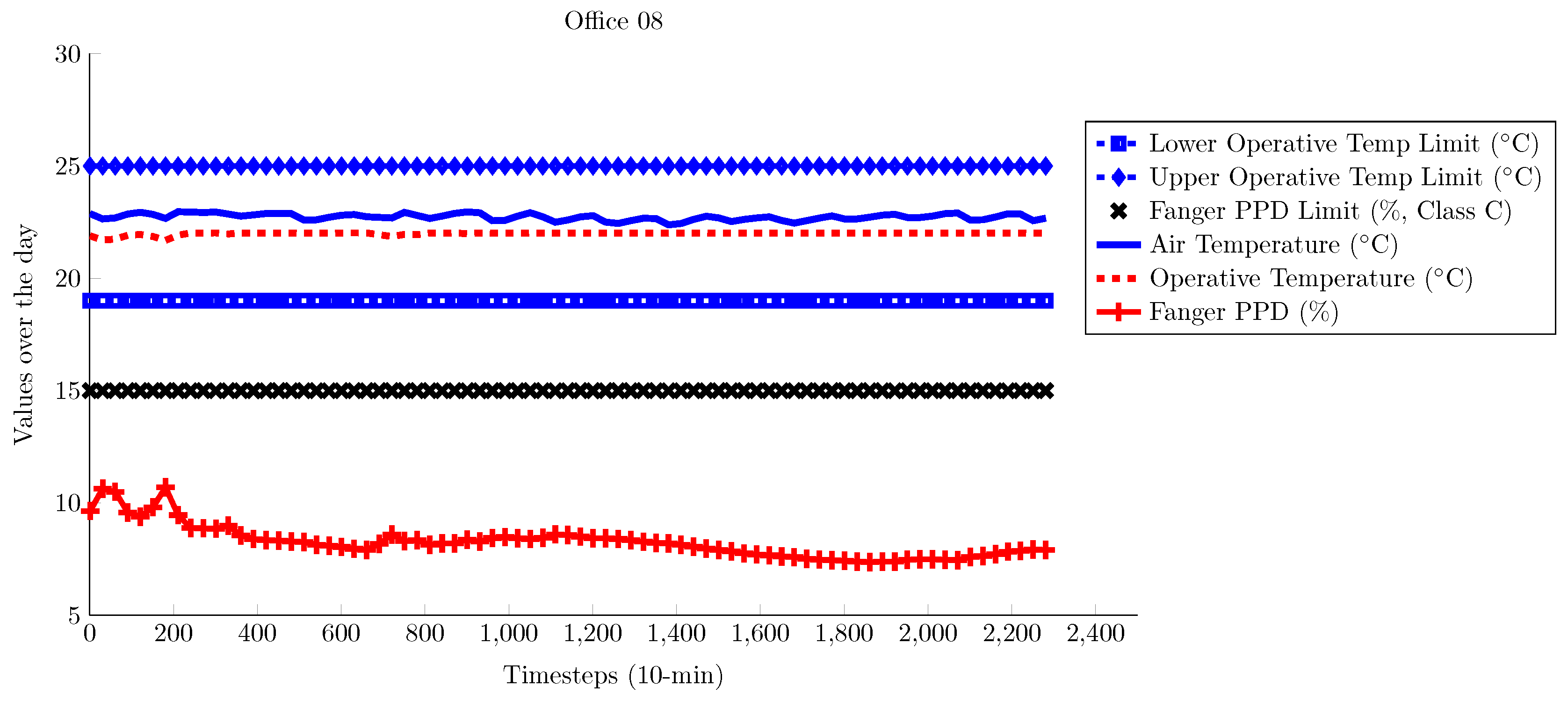
For the winter experiments, Figure 10 illustrates the results obtained for Office 08, where Fanger PPD values are within the acceptable limit for this type of building most of the time. Note here that the operative temperature is lower compared to the air temperature throughout the simulation period. This is expected, since even though the HVAC system is based on radiant heating (radiators) and a part of the heating energy is absorbed by the walls, the lightweight construction and the poor insulation of the building lead to lower wall temperatures (thus lower radiant temperature) compared to the air temperature of the zone. The relative humidity in the office varies from 30%–50% depending on the external conditions, thus affecting the comfort as with the summer experiments, with this effect being more obvious in the first two days of the experiment, where the relative humidity is around 30%.
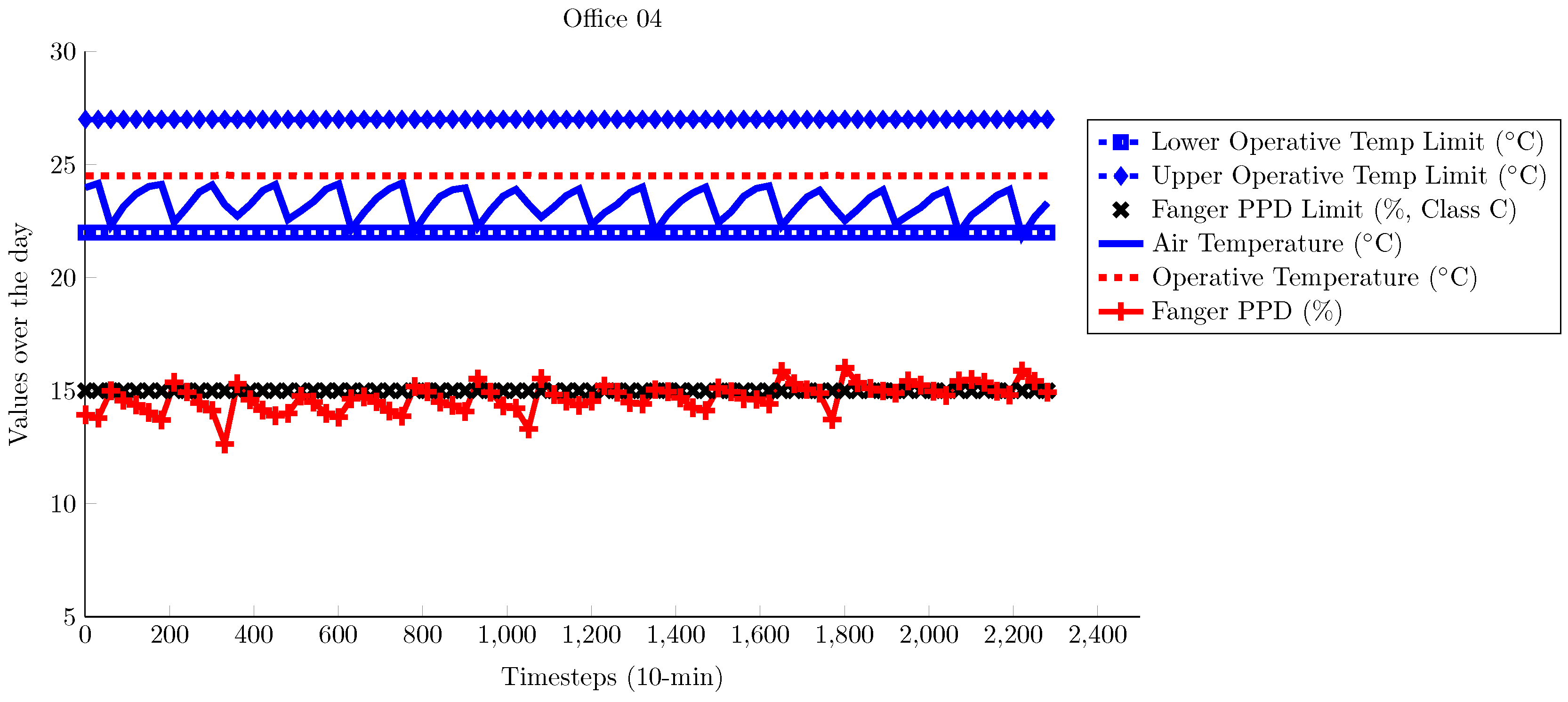
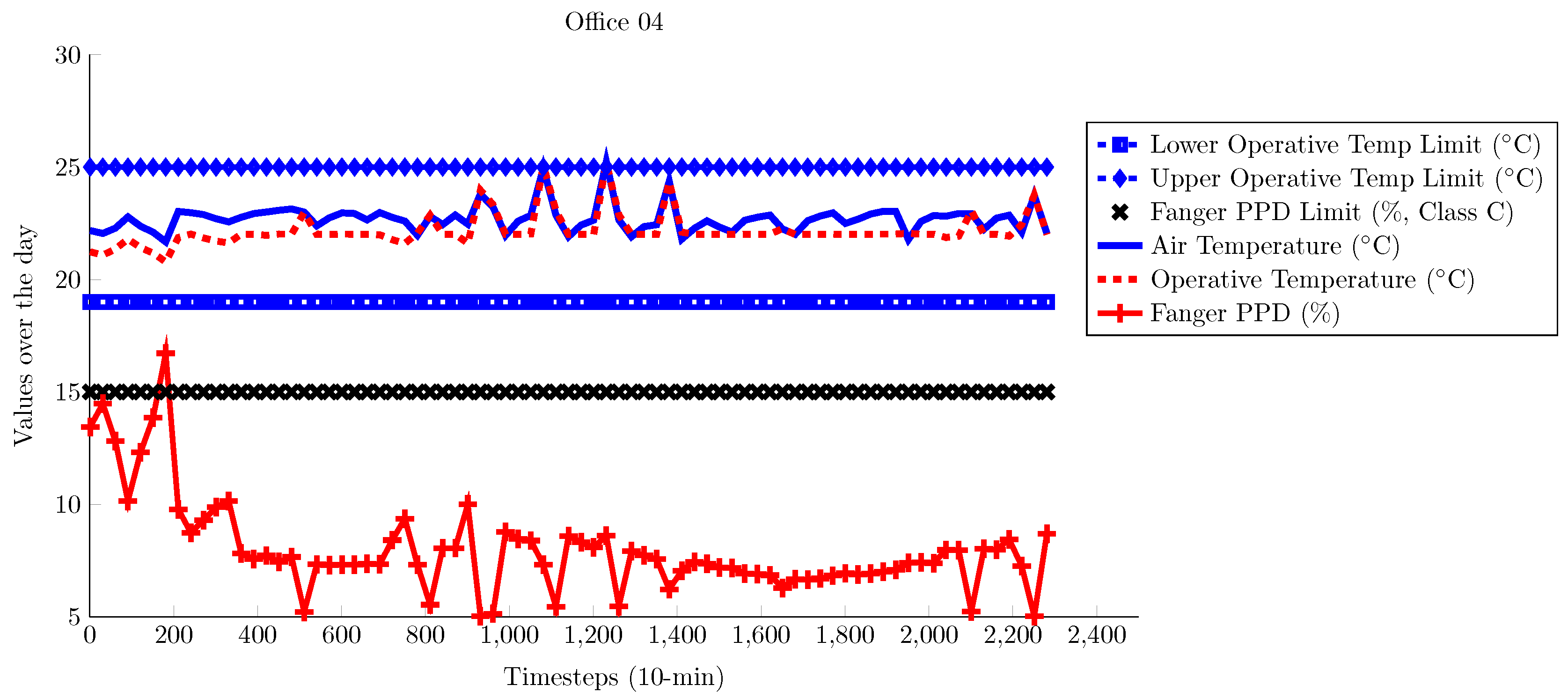
Office 04 results for the same experiment are shown in Figure 11, leading to the same conclusions: Fanger PPD values remain within acceptable limits for most of the time, while the air temperature is higher compared to the operative temperature. On the other hand, we can notice some spikes on both air and operative temperatures, which are due to the high solar gains office 04 is exposed to (unlike office 08) on days with clear sky. Note that for the first two days of the experiment, relative humidity is around 30%, thus leading to increased discomfort as in the case of office 08 above.
As with the summer set of evaluations, the same experiments are conducted controlling the operative temperature instead of the zone air temperature. Here, as illustrated in Figure 12 for Office 08, the air temperature is higher than the operative temperature as with the air temperature thermostat control, but both naturally acquire higher values compared to the previous experiment for the same office (Figure 10), which leads to more comfortable interior conditions as indicated by the Fanger PPD levels.
The same comfort improvement due to the increased values of operative temperature is also observed in Office 04 results (Figure 13). Of course, as with the previous winter experiment controlling the air temperature in the same office (Figure 11), both operative and air temperatures show periodic increments due to the high solar gains on less cloudy days.
The results from these experiments confirm our initial hypotheses: (i) controlling the air temperature does not provide a structured method for controlling the operative temperature; and (ii) the suggested operative temperature comfort band calculated in ISO 7730 for a fixed clo value, metabolic rate and relative humidity levels needs to be adapted to the particularities of each target building.
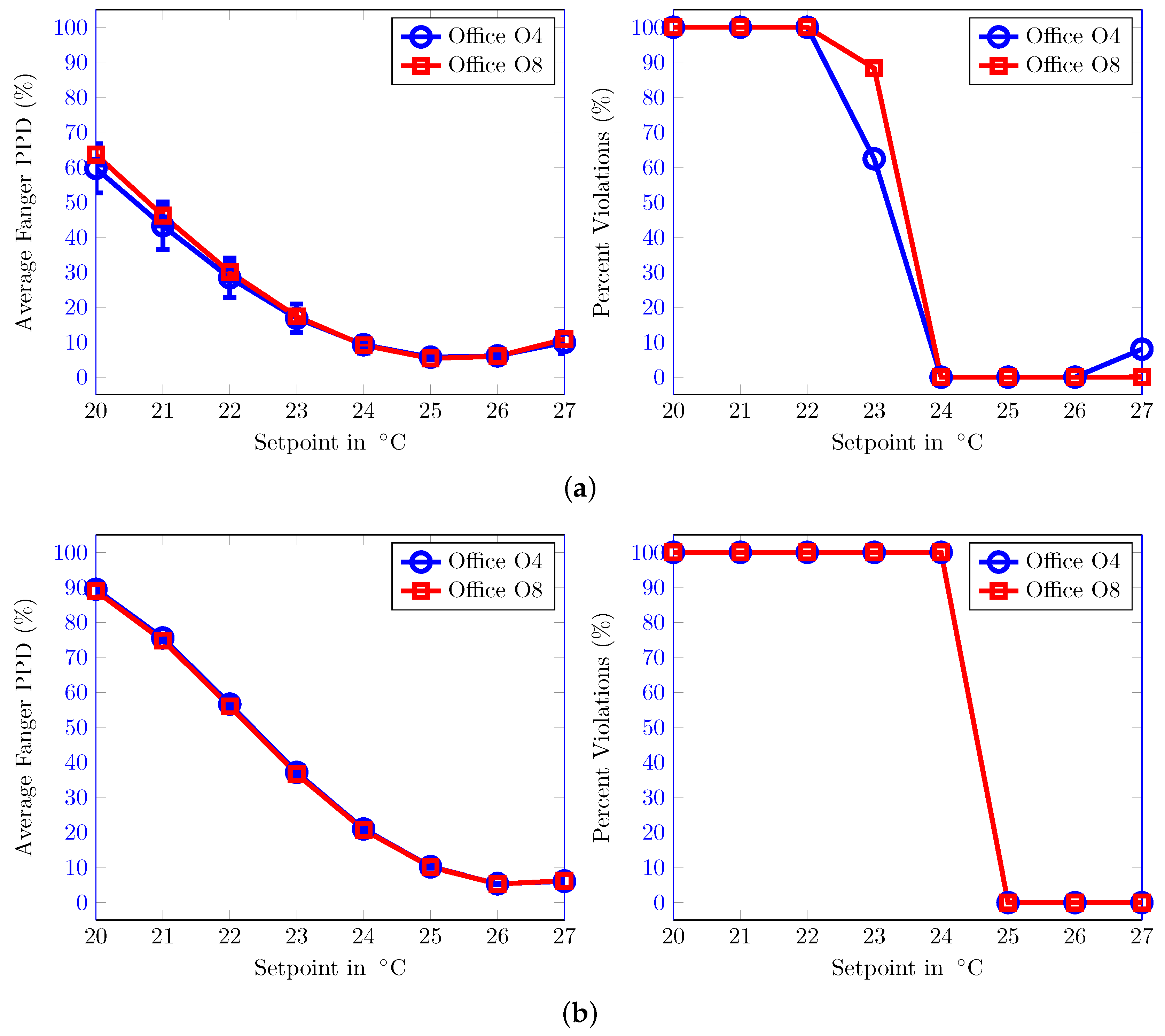
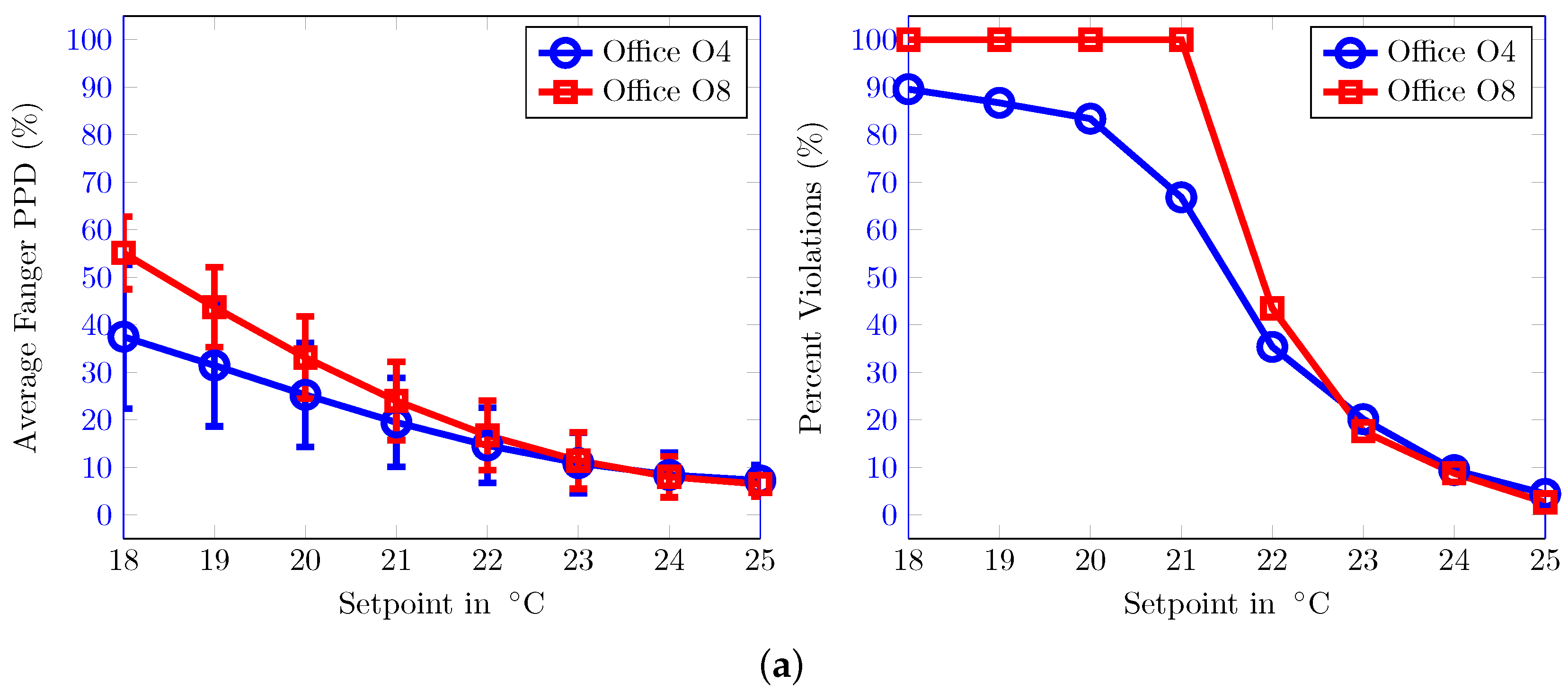
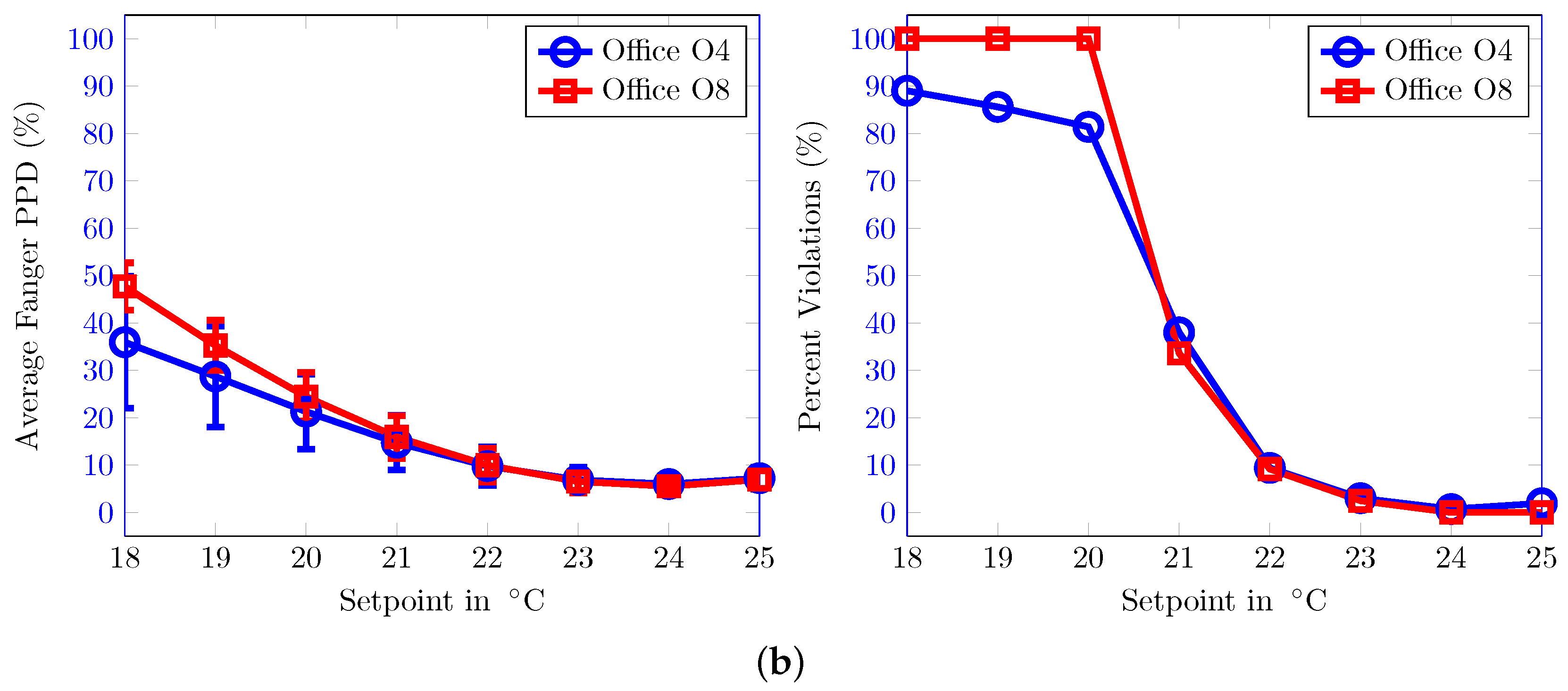
In order to provide a clear illustration of the difference in the thermal comfort conditions between air and operative temperature control in the TUC building, a parametric study for the same summer and winter days as before and with different air and operative temperature set-points has been performed. The impact on comfort is evaluated using both the percentage of comfort violations and the average Fanger PPD values in the entire experimental period. For the latter, the standard deviation of the Fanger PPD values is also presented to provide an estimate of the variability of the comfort levels throughout the experiment. The results for all cases are shown in Figure 14 and Figure 15 for Offices 04 and 08 as before and for summer and winter, respectively.
For the summer study, the inequivalence of the two control strategies (air over operative temperature) is apparent, since for the air temperature control, all set-points between 24 °C and 26 °C lead to comfortable interiors for both offices, while for the operative temperature, this interval is shifted between 25 °C and 27 °C.
The same conclusion is derived from the winter results, since here, the best air temperature set-point is 25 °C, while it is 24 °C for the operative temperature. Apart from this, another interesting observation here is the high variability of the Fanger PPD values (as indicated by the high standard deviation) due to the internal occupant and equipment gains and, mostly for Office 04, the solar gains throughout the entire simulation period, as well as the slow dynamics of the heating system (radiators).
Concluding with the experiments conducted in the TUC building, we have been able to confirm the inability of widely-used air temperature control methodologies to provide a structured and systematic way of representing and controlling thermal comfort in buildings, as well as the necessity to constantly adapt thermal comfort constraints based on the actual environmental (humidity) and personal (e.g., clo value) influencing factors, rather than myopically adopting the (calculated under steady-state conditions) operative temperature constraints in the example tables included in ISO 7730.
4.2. ZUB Building
In the ZUB building, only winter experiments are performed using air temperature thermostat control. The period between 25 January and 4 February is selected, while a Meteonorm weather file [59] is used. In this period, we have some days with clear sky, with the average temperature at 3.3 °C, the minimum temperature at −5.4 °C and the maximum temperature at 9.3 °C.
In contrast to the experiments conducted in the TUC building, the ZUB building is intended to serve as a test bed complying with the assumptions leading to Table 1 of ISO 7730. In this direction, an ideal ventilation system with a fixed airflow of 50% relative humidity has been implemented in all offices and the atrium. In order to not affect the room temperature and the energy balance, the ventilated air (with an air-change rate of 0.7 1/h) has the same temperature as the respective room temperature. In reality, the building is not equipped with a de-/humidification system, so this approach is a theoretic workaround to obtain the desired humidity levels. In the same direction, although an airflow model (TRNFlow) of the building is available, it is disabled for this study to limit the disturbances affecting comfort. Instead, an infiltration rate of 0.1 1/h has been set for all offices due to cracks and openings in the building. Finally, the same clo value assumed in ISO 7730 has been defined in all experiments.
Here, a simple control approach was chosen. Each room has an on/off differential controller, which is acting as a thermostat. The controller tries to maintain a user-defined set temperature within a certain dead band (±1 °C) by switching the TABS-mass flow on or off. An internal hysteresis is used to prevent oscillation, while the hot water sending temperature in this case depends on the mean ambient temperature over the last 24 h through a heating curve defined for the building [60].
In these experiments, windows are considered always closed, while the blinds are activated when the total radiation on the main facade rises above 500 W/m2, and they are deactivated when it falls below 300 W/m2. Here, closed blinds result in a reduction of the solar radiation in an office by 70%. The air temperature thermostat set-point is set at 21 °C (lower limit for Class A buildings according to ISO 7730; see Table 1), implemented using the controller described above.
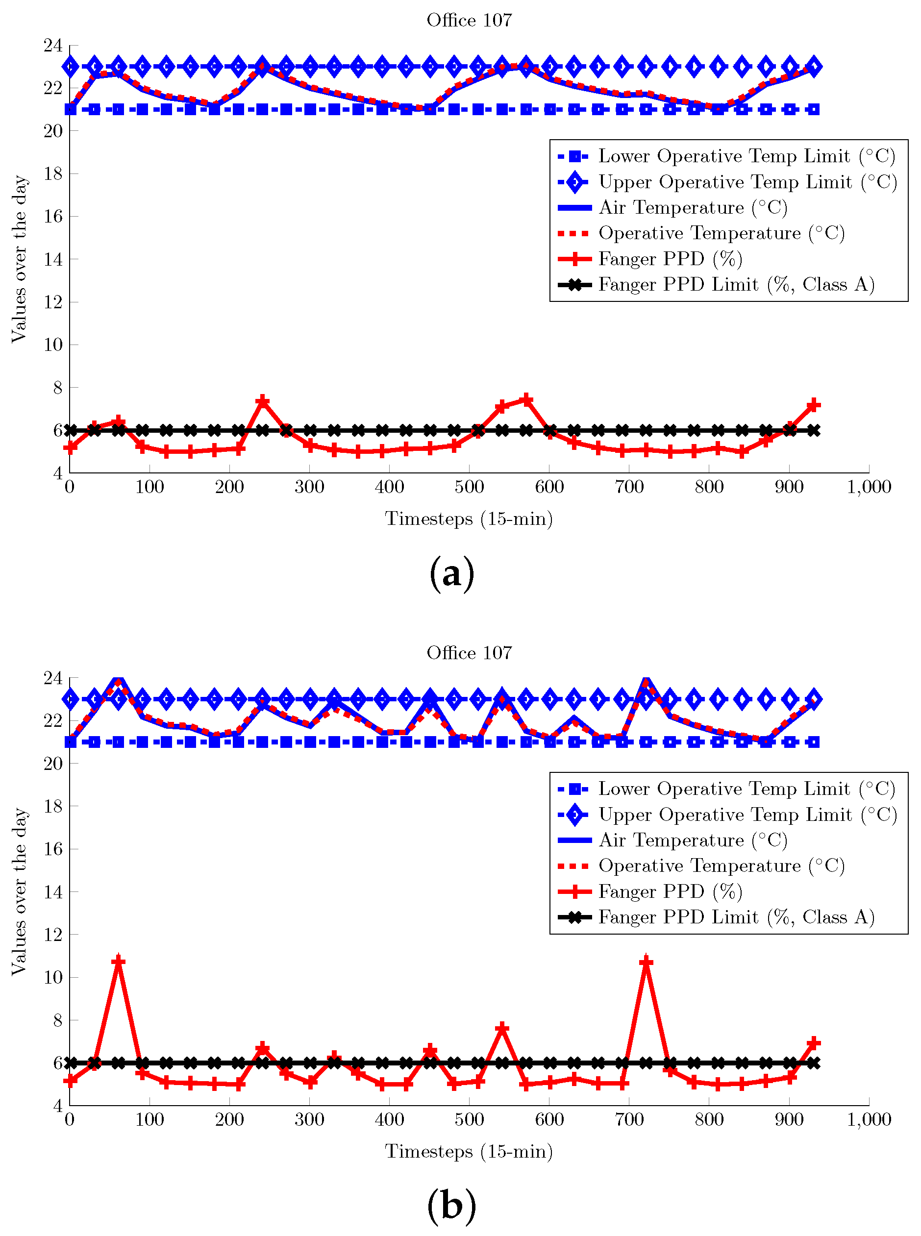
For the ZUB building, two sets of air temperature control experiments are conducted, with the results shown in Figure 16, only for Office 107. The first setting forces the blinds always closed and no internal gains in order to ensure steady-state operation of the TABS, while the second includes internal gains and uses the default blinds control strategy of the building as described earlier. For both cases, the air and operative temperatures coincide, due to the dynamics of the system and the heavy construction and insulation of the building. On the other hand, Figure 16b reveals the well-known overheating problem of buildings equipped with TABS due to internal and solar gains [39,61], indicating the utilization of solutions facilitating weather and occupancy forecasts [2,16,39] as an attractive option for control.
5. Conclusions
In the present work, an investigation on the ability of room thermostats to ensure comfortable building interiors has been performed. The wide use of such controllers is mainly based on two assumptions: (i) that the operative temperature limits for comfortable interiors defined in ISO 7730 suffice to ensure user thermal comfort; and (ii) that air and operative temperatures of building interiors coincide.
Regarding the first assumption, simulation results for an existing building in Crete indicate that neglecting other parameters influencing thermal sensation and designing controllers based on the indicative operative temperature limits of ISO 7730 can lead to invalid thermal sensation estimates. More importantly, the necessity for controlling (or at least accounting for) the humidity in building spaces has proven a crucial ingredient towards accurate estimation of thermal sensation and, thus, towards efficient control of building indoor climate.
For the second assumption, experimental validation on the same building revealed an appreciable mismatch between indoor air and operative temperatures for both summer and winter tests, due to the dynamics of the HVAC system in each case (radiators for heating and PTHP for cooling season) and the construction and thermal properties of the building. On the other hand, we observed similar air and operative temperature values on a heavy construction building equipped with TABS leading to the conclusion that for specific construction and HVAC system dynamics, the air temperature measurements provide an accurate enough estimation of the operative temperature. Here, we can generalize that for buildings with high thermal mass, this assumption holds, if proper care is taken to account for solar and internal gains in the control strategy, while as we move to buildings with lower thermal mass, there can be a considerable mismatch between air and operative temperatures in building spaces.
In connection with studies that model the user behaviour in buildings, the work presented here indicates that in many cases, the users interact with the controllable building elements in order to restore comfortable interiors, due to the wrong estimation of thermal comfort in their spaces. This suggests that the ability to calculate comfort indices such as Fanger, or even the ability to build personalized comfort models for the building occupants [62,63,64,65,66] can enable a more comfort-aware and user-centric building design and operation. Here, building designers and energy modellers can estimate more accurately the future energy consumption of a building, by taking into account the energy required to ensure comfortable interiors (through proper control actions), instead of using fixed temperature set-points throughout yearly simulations. In a similar manner, the realization from building operators that thermal comfort is not synonymous with pre-defined indoor air temperature bounds can enable them to control the buildings in a more thermal comfort-aware manner, thus minimizing user requests for adaptation of their local environment and leading to increased productivity. To this end, in buildings where proper sensor installation for calculating comfort indices like Fanger is missing, a simulation model of the building (or of specific building spaces) can be utilized as a virtual sensor, providing accurate thermal comfort estimations through, e.g., simulation-based Fanger calculation [67].
Finally, compared to existing standards, the DNAS (Drivers, Needs, Actions, Systems) framework (developed within IEA Annex 66) is meant to highlight a way forward, as it captures the subjectivity of user actions and highlights something that is now beginning to emerge and be understood: user actions are subjective and influenced by specific drivers. As demonstrated in various studies outside the domain of human comfort in buildings (which involved engineers, but also anthropologists and psychologists), users exhibit an ordinal set of preferences with respect to the various actions they have to takes and make decisions based on specific drivers. Establishing such an ordinal relationship can be key to user modelling. This is different from the accepted notion that a simple statistical index might act as a universal approximator of comfort sensation. Furthermore the fallacy of the assumption that comfort can be estimated simply by a single point measurement (typically dry bulb temperature), highlighted in this paper, partly explains the irrationality of the current state of practice with respect to building control. Towards shaping a new generation of standards, the DNAS framework (developed within IEA Annex 66) and the implicit assumption of ordinal preference learning should be key considerations underpinning the development of such standards.
Acknowledgments
The authors would like to express their gratitude to Martin Felix Pichler and Hermann Schranzhofer of Graz University of Technology for providing the initial version of the ZUB TRNSYS model within the Positive Energy Buildings thru Better Control Decisions (PEBBLE) FP7 Project (FP7-ICT-2007-9.6.3, Grant #248537). We also thank Juan Rodriguez Santiago of Fraunhofer Institute for Wind Energy and Energy System Technology (IWES) Kassel for many helpful discussions regarding ZUB building operation. Research leading to these results has been partially supported by FP7-ICT-2011-6: Building as a Service (BaaS, #288409). Georgios Kontes gratefully acknowledges financial support from the Modelling Optimization of Energy Efficiency in Buildings for Urban Sustainability (MOEEBIUS) project, a Horizon 2020 research and innovation program under Grant Agreement #680517. Georgios Kontes and Simone Steiger gratefully acknowledge use of the services and facilities of the Energie Campus Nürnberg and financial support through the “Aufbruch Bayern (Bavaria on the move)” initiative of the state of Bavaria. Georgios Giannakis and Dimitrios Rovas gratefully acknowledge financial support from the European Commission H2020-EeB5-2015 project “Optimised Energy Efficient Design Platform for Refurbishment at District Level” under Contract #680676 (OptEEmAL).
Author Contributions
Georgios Kontes designed the experiments and analysed the results, with the support of Georgios Giannakis and Philip Horn. Georgios Giannakis set up the EnergyPlus simulations for the TUC building and Philip Horn the TRNSYS simulations for the ZUB building. Georgios Kontes, Georgios Giannakis and Philip Horn wrote the paper. Simone Steiger proofread the paper and helped improve various sections in the text, in addition to offering key insights into the interpretation of the results. Dimitrios Rovas oversaw the entire work, offered key insights in the design and extension of the experiments and the analysis of the results and proofread the paper.
Conflicts of Interest
The authors declare no conflict of interest.
References
- Pichler, M.; Droscher, A.; Schranzhofer, H.; Kontes, G.; Giannakis, G.; Kosmatopoulos, E.; Rovas, D. Simulation-assisted building energy performance improvement using sensible control decisions. In Proceedings of the 3rd ACM Workshop on Embedded Sensing Systems for Energy-Efficiency in Buildings, Seattle, WA, USA, 1 November 2011. [Google Scholar]
- Oldewurtel, F.; Parisio, A.; Jones, C.; Gyalistras, D.; Gwerder, M.; Stauch, V.; Lehmann, B.; Morari, M. Use of model predictive control and weather forecasts for energy efficient building climate control. Energy Build. 2012, 45, 15–27. [Google Scholar] [CrossRef]
- Zavala, V.M. Real-Time Optimization Strategies for Building Systems. Ind. Eng. Chem. Res. 2012, 52, 3137–3150. [Google Scholar] [CrossRef]
- Ghahramani, A.; Zhang, K.; Dutta, K.; Yang, Z.; Becerik-Gerber, B. Energy savings from temperature set-points and deadband: Quantifying the influence of building and system properties on savings. Appl. Energy 2016, 165, 930–942. [Google Scholar] [CrossRef]
- Kontogianni, E.; Giannakis, G.; Kontes, G.; Rovas, D. Comparing the Impact of Different Thermal Comfort Constraints on a Model-Assisted Control Design Process. In Proceedings of the 11th REHVA World Congress, Prague, Czech Republic, 16–19 June 2013. [Google Scholar]
- Morales-Valdés, P.; Flores-Tlacuahuac, A.; Zavala, V.M. Analyzing the effects of comfort relaxation on energy demand flexibility of buildings: A multiobjective optimization approach. Energy Build. 2014, 85, 416–426. [Google Scholar] [CrossRef]
- Fisk, W.J. Health and productivity gains from better indoor environments and their relationship with building energy efficiency. Ann. Rev. Energy Environ. 2000, 25, 537–566. [Google Scholar] [CrossRef]
- Akimoto, T.; Tanabe, S.I.; Yanai, T.; Sasaki, M. Thermal comfort and productivity-Evaluation of workplace environment in a task conditioned office. Build. Environ. 2010, 45, 45–50. [Google Scholar] [CrossRef]
- International Organization for Standardization. ISO7730:2005: Ergonomics of the Thermal Environment—Analytical Determination and Interpretation of Thermal Comfort Using Calculation of the PMV and PPD Indices and Local Thermal Comfort Criteria; International Organization for Standardization: Geneva, Switzerland, 2005. [Google Scholar]
- European Committee for Standardization (CEN). EN15251: Indoor Environmental Input Parameters for Design and Assessment of Energy Performance of Buildings—Addressing Indoor Air Quality, Thermal Environment, Lighting and Acoustics; CEN: Brussels, Belgium, 2007. [Google Scholar]
- American Society of Heating, Refrigerating and Air-Conditioning Engineers (ASHRAE). ANSI/ASHRAE Standard 55-2010: Thermal Environmental Conditions for Human Occupancy; ASHRAE: Atlanta, GA, USA, 2010. [Google Scholar]
- Donaisky, E.; Oliveira, G.H.; Freire, R.Z.; Mendes, N. PMV-based predictive algorithms for controlling thermal comfort in building plants. In Proceedings of the IEEE International Conference on Control Applications, CCA 2007, Singapore, 1–3 October 2007. [Google Scholar]
- Freire, R.Z.; Oliveira, G.H.; Mendes, N. Predictive controllers for thermal comfort optimization and energy savings. Energy Build. 2008, 40, 1353–1365. [Google Scholar] [CrossRef]
- Cigler, J.; Prívara, S.; Váňa, Z.; Žáčeková, E.; Ferkl, L. Optimization of predicted mean vote index within model predictive control framework: Computationally tractable solution. Energy Build. 2012, 52, 39–49. [Google Scholar] [CrossRef]
- Drgona, J.; Kvasnica, M.; Klauco, M.; Fikar, M. Explicit stochastic MPC approach to building temperature control. In Proceedings of the 52nd Annual Conference on Decision and Control (CDC), Florence, Italy, 10–13 December 2013. [Google Scholar]
- Kontes, G.; Valmaseda, C.; Giannakis, G.; Katsigarakis, K.; Rovas, D. Intelligent BEMS design using detailed thermal simulation models and surrogate-based stochastic optimization. J. Process Control 2014, 24, 846–855. [Google Scholar] [CrossRef]
- Katsigarakis, K.; Kontes, G.; Giannakis, G.; Rovas, D. Sense-Think-Act Framework for Intelligent Building Energy Management. Comput. -Aided Civ. Infrastruct. Eng. 2016, 31, 50–64. [Google Scholar] [CrossRef]
- Mařík, K.; Rojíček, J.; Stluka, P.; Vass, J. Advanced HVAC control: Theory vs. reality. In Proceedings of the 18th IVAC World Congress, Milano, Italy, 28 August–2 September 2011. [Google Scholar]
- Moon, J.W.; Han, S.H. Thermostat strategies impact on energy consumption in residential buildings. Energy Build. 2011, 43, 338–346. [Google Scholar] [CrossRef]
- Hoyt, T.; Arens, E.; Zhang, H. Extending air temperature set-points: Simulated energy savings and design considerations for new and retrofit buildings. Build. Environ. 2015, 88, 89–96. [Google Scholar] [CrossRef]
- Ma, Y.; Kelman, A.; Daly, A.; Borrelli, F. Predictive Control for Energy Efficient Buildings with Thermal Storage: Modeling, Stimulation, and Experiments. IEEE Control Syst. 2012, 32, 44–64. [Google Scholar] [CrossRef]
- Atam, E.; Helsen, L. Control-Oriented Thermal Modeling of Multizone Buildings: Methods and Issues: Intelligent Control of a Building System. IEEE Control Syst. 2016, 36, 86–111. [Google Scholar] [CrossRef]
- D’Oca, S.; Fabi, V.; Corgnati, S.P.; Andersen, R.K. Effect of thermostat and window opening occupant behavior models on energy use in homes. Build. Simul. 2014, 7, 683–694. [Google Scholar] [CrossRef]
- Li, C.; Hong, T.; Yan, D. An insight into actual energy use and its drivers in high-performance buildings. Appl. Energy 2014, 131, 394–410. [Google Scholar] [CrossRef]
- Azar, E.; Menassa, C.C. Evaluating the impact of extreme energy use behavior on occupancy interventions in commercial buildings. Energy Build. 2015, 97, 205–218. [Google Scholar] [CrossRef]
- IEA Annex 66. Definition and Simulation of Occupant Behavior in Buildings. Available online: www.annex66.org (accessed on 8 September 2017).
- Hong, T.; D’Oca, S.; Turner, W.J.; Taylor-Lange, S.C. An ontology to represent energy-related occupant behavior in buildings. Part I: Introduction to the DNAs framework. Build. Environ. 2015, 92, 764–777. [Google Scholar] [CrossRef]
- Gunay, H.B.; O’Brien, W.; Beausoleil-Morrison, I.; Bursill, J. Development and implementation of a thermostat learning algorithm. Sci. Technol. Built Environ. 2017, 1–14. [Google Scholar] [CrossRef]
- Haldi, F.; Robinson, D. On the behaviour and adaptation of office occupants. Build. Environ. 2008, 43, 2163–2177. [Google Scholar] [CrossRef]
- Haldi, F.; Robinson, D. Interactions with window openings by office occupants. Build. Environ. 2009, 44, 2378–2395. [Google Scholar] [CrossRef]
- Yun, G.Y.; Tuohy, P.; Steemers, K. Thermal performance of a naturally ventilated building using a combined algorithm of probabilistic occupant behaviour and deterministic heat and mass balance models. Energy Build. 2009, 41, 489–499. [Google Scholar] [CrossRef] [Green Version]
- Nagy, Z.; Yong, F.Y.; Frei, M.; Schlueter, A. Occupant centered lighting control for comfort and energy efficient building operation. Energy Build. 2015, 94, 100–108. [Google Scholar] [CrossRef]
- Ghahramani, A.; Jazizadeh, F.; Becerik-Gerber, B. A knowledge based approach for selecting energy-aware and comfort-driven HVAC temperature set points. Energy Build. 2014, 85, 536–548. [Google Scholar] [CrossRef]
- Romero, A.; Tellado, B.; Tsitsanis, T. MOEEBIUS energy performance optimization framework in buildings for urban sustainability. In Proceedings of the 41st IAHS World Congress, Albufeira, Portugal, 13–16 September 2016. [Google Scholar]
- Baker, L.; Hoyt, T. Control for the People: How Machine Learning Enables Efficient HVAC Use Across Diverse Thermal Preferences. In Proceedings of the ACEEE Summer Study on Energy Efficiency in Buildings, Pacific Grove, CA, USA, 13–18 August 2016. [Google Scholar]
- Kang, D.H.; Mo, P.H.; Choi, D.H.; Song, S.Y.; Yeo, M.S.; Kim, K.W. Effect of MRT variation on the energy consumption in a PMV-controlled office. Build. Environ. 2010, 45, 1914–1922. [Google Scholar] [CrossRef]
- Marino, C.; Nucara, A.; Pietrafesa, M. Mapping of the indoor comfort conditions considering the effect of solar radiation. Solar Energy 2015, 113, 63–77. [Google Scholar] [CrossRef]
- Lehmann, B.; Dorer, V.; Koschenz, M. Application range of thermally activated building systems tabs. Energy Build. 2007, 39, 593–598. [Google Scholar] [CrossRef]
- Gwerder, M.; Lehmann, B.; Tödtli, J.; Dorer, V.; Renggli, F. Control of thermally-activated building systems (TABS). Appl. energy 2008, 85, 565–581. [Google Scholar] [CrossRef]
- Gwerder, M.; Tödtli, J.; Lehmann, B.; Dorer, V.; Güntensperger, W.; Renggli, F. Control of thermally activated building systems (TABS) in intermittent operation with pulse width modulation. Appl. Energy 2009, 86, 1606–1616. [Google Scholar] [CrossRef]
- Feng, J.D.; Chuang, F.; Borrelli, F.; Bauman, F. Model predictive control of radiant slab systems with evaporative cooling sources. Energy Build. 2015, 87, 199–210. [Google Scholar] [CrossRef]
- Fanger, P.O. Thermal Comfort: Analysis and Applications in Environmental Engineering; Danish Technical Press: Vanloese, Denmark, 1970. [Google Scholar]
- Ma, Y.; Borrelli, F.; Hencey, B.; Coffey, B.; Bengea, S.; Haves, P. Model predictive control for the operation of building cooling systems. IEEE Trans. Control Syst. Technol. 2012, 20, 796–803. [Google Scholar]
- Azer, N.; Hsu, S. The prediction of thermal sensation from simple model of human physiological regulatory response. ASHRAE Trans. 1977, 83, 88–102. [Google Scholar]
- Gagge, A. An effective temperature scale based on a simple model of human physiological regulatory response. ASHRAE Trans. 1971, 77, 247–262. [Google Scholar]
- International Organization for Standardization. ISO8996:1989: Ergonomics of Thermal Environments—Determination of Metabolic Heat Production; International Organization for Standardization: Geneva, Switzerland, 1989. [Google Scholar]
- Schiavon, S.; Lee, K.H. Dynamic predictive clothing insulation models based on outdoor air and indoor operative temperatures. Build. Environ. 2013, 59, 250–260. [Google Scholar] [CrossRef]
- Schiavon, S.; Hoyt, T.; Piccioli, A. Web application for thermal comfort visualization and calculation according to ASHRAE Standard 55. Build. Simul. 2014, 7, 321–334. [Google Scholar] [CrossRef]
- Crawley, D.; Lawrie, L.; Winkelmann, F.; Buhl, W.; Huang, Y.; Pedersen, C.; Strand, R.; Liesen, R.; Fisher, D.; Witte, M.; et al. EnergyPlus: creating a new-generation building energy simulation program. Energy Build. 2001, 33, 319–331. [Google Scholar] [CrossRef]
- Walton, G. AIRNET: A Computer Program for Building Airflow Network Modeling; US Dept. of Commerce, National Institute of Standards and Technology, National Engineering Laborary, Center for Building Research, Building Environment Division: Washington D.C., WA, USA, 1989.
- Woods, J.; Winkler, J.; Christensen, D. Evaluation of the Effective Moisture Penetration Depth Model for Estimating Moisture Buffering in Buildings. NREL/TP-5500-57441; National Renewable Energy Laboratory (NREL): Golden, CO, USA, 1 January 2013. [Google Scholar]
- Droscher, A.; Schranzhofer, H.; Santiago, J.; Constantin, A.; Streblow, R.; Muller, D.; Exizidou, P.; Giannakis, G.; Rovas, D. Integrated Thermal Simulation Models for the Three Buildings. In PEBBLE Deliverable 2.1; Technical University of Crete (TUC): Chania, Greece, 2010. [Google Scholar]
- Klein, S.; Beckman, W.; Duffie, J. TRNSYS—A Transient Simulation Program. ASHRAE Trans. 1976, 82, 623–633. [Google Scholar]
- Giannakis, G.; Pichler, M.; Kontes, G.; Schranzhofer, H.; Rovas, D. Simulation speedup techniques for computationally demanding tasks. Proceedings of BS 2013: 13th Conference of the International Building Performance Simulation Association, Chambéry, France, 26–28 August 2013. [Google Scholar]
- Verein Deutscher Ingenieure. Berechnung der Kühllast Klimatisierter Räume (VDI-Kühllastregeln); Verein Deutscher Ingenieure: Dusseldorf, Germany, 1977. [Google Scholar]
- Judkoff, R.; Neymark, J. International Energy Agency Building Energy Simulation Test (BESTEST) and Diagnostic Method; Technical Report; National Renewable Energy Lab: Golden, CO, USA, 1995. [Google Scholar]
- Neymark, J.; Judkoff, R.; Knabe, G.; Le, H.T.; Dürig, M.; Glass, A.; Zweifel, G. Applying the building energy simulation test (BESTEST) diagnostic method to verification of space conditioning equipment models used in whole-building energy simulation programs. Energy Build. 2002, 34, 917–931. [Google Scholar] [CrossRef]
- Maasoumy, M.; Vincentelli, A.S. Comparison of control strategies for energy efficient building HVAC systems. In Proceedings of the Symposium on Simulation for Architecture & Urban Design, Tampa, FL, USA, 13–16 April 2014. [Google Scholar]
- Remund, J.; Kunz, S.; Lang, R. METEONORM-Global meteorological database for solar energy and applied climatology. In Solar Engineering Handbook, Version 4.0; Meteotest: Bern, Switzerland, 1999. [Google Scholar]
- Rovas, D.; Kontes, G.; Valmaseda, C.; Giannakis, G.; Chacel, O.; Macek, K.; Fisera, R.; Rojicek, J.; Hottges, K.; Menzel, K.; Floeck, M. BaaS Advanced Use Cases. BAAS Deliverable 5.1b. 2014. [Google Scholar]
- Olesen, B.W. Radiant floor heating in theory and practice. ASHRAE J. 2002, 44, 19–26. [Google Scholar]
- Daum, D.; Haldi, F.; Morel, N. A personalized measure of thermal comfort for building controls. Build. Environ. 2011, 46, 3–11. [Google Scholar] [CrossRef]
- Ghahramani, A.; Tang, C.; Becerik-Gerber, B. An online learning approach for quantifying personalized thermal comfort via adaptive stochastic modeling. Build. Environ. 2015, 92, 86–96. [Google Scholar] [CrossRef]
- Malavazos, C.; Tsatsakis, K.; Tsitsanis, A. Towards a “context aware” flexibility profiling mechanism for the energy management environment. In Proceedings of the MedPower Conference, Athens, Greece, 2–5 November 2014. [Google Scholar]
- Sadeghi, S.A.; Awalgaonkar, N.M.; Karava, P.; Bilionis, I. A Bayesian modeling approach of human interactions with shading and electric lighting systems in private offices. Energy Build. 2017, 134, 185–201. [Google Scholar] [CrossRef]
- Lee, S.; Bilionis, I.; Karava, P.; Tzempelikos, A. A Bayesian approach for probabilistic classification and inference of occupant thermal preferences in office buildings. Build. Environ. 2017, 118, 323–343. [Google Scholar] [CrossRef]
- Pang, X.; Wetter, M.; Bhattacharya, P.; Haves, P. A framework for simulation-based real-time whole building performance assessment. Build. Environ. 2012, 54, 100–108. [Google Scholar] [CrossRef]
Figure 1.
Acceptable range of operative temperature and humidity ratio based on ASHRAE Standard 55 [11]. The chart was created using the Center for the Built Environment (CBE) Thermal Comfort Tool [48]. clo, clothing value.

Figure 2.
The TUC building. (a) TUC building designed with Open Studio plugin; (b) ground floor plan view; and (c) first floor plan view.
Figure 2.
The TUC building. (a) TUC building designed with Open Studio plugin; (b) ground floor plan view; and (c) first floor plan view.

Figure 3.
ZUB building and simplified tower model views: (a) External view of the ZUB building; (b) full-scale simulation model of the ZUB building; and (c) southeast view of the tower model with external shading groups.
Figure 3.
ZUB building and simplified tower model views: (a) External view of the ZUB building; (b) full-scale simulation model of the ZUB building; and (c) southeast view of the tower model with external shading groups.

Figure 4.
Summer results for Office 08 using the air temperature thermostat set at 24.5 °C.

Figure 5.
Summer results for Office 04 using the air temperature thermostat set at 24.5 °C.

Figure 6.
Summer results for Office 08 using the operative temperature thermostat set at 24.5 °C.

Figure 7.
Summer results for Office 04 using the operative temperature thermostat set at 24.5 °C.

Figure 8.
Summer results for Office 08 using the operative temperature thermostat set at 25.5 °C.

Figure 9.
Summer results for Office 04 using the operative temperature thermostat set at 25.5 °C.

Figure 10.
Winter results for Office 08 using the air temperature thermostat set at 22 °C.

Figure 11.
Winter results for office 04 using air temperature thermostat set at 22 °C.

Figure 12.
Winter results for Office 08 using the operative temperature thermostat set at 22 °C.

Figure 13.
Winter results for Office 04 using operative temperature thermostat set at 22 °C.

Figure 14.
Summer experiments with different set-points. (a) User comfort evaluation for different air temperature set-points for the summer period; and (b) user comfort evaluation for different operative temperature set-points for the summer period.
Figure 14.
Summer experiments with different set-points. (a) User comfort evaluation for different air temperature set-points for the summer period; and (b) user comfort evaluation for different operative temperature set-points for the summer period.

Figure 15.
Winter experiments with different set-points. (a) User comfort evaluation for different air temperature set-points for the winter period; and (b) user comfort evaluation for different operative temperature set-points for the winter period.
Figure 15.
Winter experiments with different set-points. (a) User comfort evaluation for different air temperature set-points for the winter period; and (b) user comfort evaluation for different operative temperature set-points for the winter period.


Figure 16.
Results for Office 107 of the ZUB building: (a) Results for Office 107 using the air temperature thermostat set at 22 °C, blinds always closed and no internal gains; and (b) results for Office 107 using the air temperature thermostat set at 22 °C.
Figure 16.
Results for Office 107 of the ZUB building: (a) Results for Office 107 using the air temperature thermostat set at 22 °C, blinds always closed and no internal gains; and (b) results for Office 107 using the air temperature thermostat set at 22 °C.


Table 1.
Acceptable operative temperature and operative temperature band for thermal comfort in office buildings based on ISO 7730 [9]. PPD, Predicted Percentage of Dissatisfied people; PMV, Predictive Mean Vote.
Table 1.
Acceptable operative temperature and operative temperature band for thermal comfort in office buildings based on ISO 7730 [9]. PPD, Predicted Percentage of Dissatisfied people; PMV, Predictive Mean Vote.
| Category | Thermal Comfort Indices | Operative Temperature (°C) | Max Air Velocity (m/s) | |||
|---|---|---|---|---|---|---|
| PPD (%) | PMV | Summer | Winter | Summer | Winter | |
| A | ≤6 | [−0.2, +0.2] | 24.5 ± 1.0 | 22.0 ± 1.0 | 0.12 | 0.10 |
| B | ≤10 | [−0.5, +0.5] | 24.5 ± 1.5 | 22.0 ± 2.0 | 0.19 | 0.16 |
| C | ≤15 | [−0.7, +0.7] | 24.5 ± 2.5 | 22.0 ± 3.0 | 0.24 | 0.21 |
© 2017 by the authors. Licensee MDPI, Basel, Switzerland. This article is an open access article distributed under the terms and conditions of the Creative Commons Attribution (CC BY) license (http://creativecommons.org/licenses/by/4.0/).
Share and Cite
MDPI and ACS Style
Kontes, G.D.; Giannakis, G.I.; Horn, P.; Steiger, S.; Rovas, D.V. Using Thermostats for Indoor Climate Control in Office Buildings: The Effect on Thermal Comfort. Energies 2017, 10, 1368. https://doi.org/10.3390/en10091368
AMA Style
Kontes GD, Giannakis GI, Horn P, Steiger S, Rovas DV. Using Thermostats for Indoor Climate Control in Office Buildings: The Effect on Thermal Comfort. Energies. 2017; 10(9):1368. https://doi.org/10.3390/en10091368
Chicago/Turabian StyleKontes, Georgios D., Georgios I. Giannakis, Philip Horn, Simone Steiger, and Dimitrios V. Rovas. 2017. "Using Thermostats for Indoor Climate Control in Office Buildings: The Effect on Thermal Comfort" Energies 10, no. 9: 1368. https://doi.org/10.3390/en10091368
Note that from the first issue of 2016, this journal uses article numbers instead of page numbers. See further details here.