Improved Krill Herd Algorithm with Novel Constraint Handling Method for Solving Optimal Power Flow Problems

Abstract

As one of the most important tools used in operation and planning of power systems, the optimal power flow (OPF) problem considering the economy and security is large-scale, complex and hard to solve. In this paper, an improved krill herd algorithm (IKHA) has been proposed. In IKHA, the onlooker search mechanism is introduced to reduce the probability of falling into local optimum; and the parameter values of the proposed algorithm including inertia weight and step-length scale factor are varied according to the iteration of evolutionary process, which improves the exploration and exploitation capabilities. Moreover, a novel constraint handling method is proposed to guide the individual to the feasible space and ensure that the optimal solution satisfies the security constraints. Then, IKHA is combined with the novel constraint handling method to solve the multi-constrained OPF problem, and its performance is tested on the IEEE 30 bus, IEEE 57 bus and IEEE 118 bus systems for 10 different simulation cases containing linear and non-linear objective functions. The simulation results demonstrate that the proposed method can solve the OPF problem successfully and obtain better solutions compared with other methods reported in the recent literatures, which prove the feasibility and effectiveness of the improvements in this work.

1. Introduction

Electricity is the main driving force of national economies and life, so it is particularly important to improve the properties of power systems, such as the safety, the reliability and the economy. Today’s electric power system is a changeable and sophisticated system due to its large scale and complicated components, including the power generation, the substations, the transmission, the power distribution and the consumption of electricity [1]. The whole society, even the whole world, should attach importance to the operation and planning of energy systems for realizing safe, reliable power system economic operation.

The optimal power flow (OPF) problem considering the economy and security is one of the most important tools used in operation and planning for energy systems [2]. The aim of OPF is to provide the optimal settings of control variables for optimizing a specific objective function, such as the generation cost function, transmission real power losses and voltage deviation, while satisfying some equality and inequality constraints. The equality constraints are power flow equations, and the inequality constraints include many limits on power system variables and operating constrains.

Initially, some traditional mathematical methods have been used to solve OPF problem, such as interior-point method [3], linear programming method [4], nonlinear programming method [5] and simplified gradient method [6]. Usually, these methods have fast calculation speed and good convergence characteristics with some restrictions on variables and objective functions. The restrictions refer to convexity, smoothness, continuity and differentiability. In fact, OPF is a large-scale, multi-constrained, non-linear and non-convex problem which contains the discrete and continuous variables. Therefore, to a certain extent, the traditional methods cannot solve the OPF problem successfully. With the development of computers, the intelligent optimization methods based on the combination of computer technology and biological simulation are proposed to overcome many drawbacks of the traditional methods; and these heuristic algorithms include artificial bee colony algorithm (ABC) [7], particle swarm optimization (PSO) [8], differential search algorithm (DSA) [9], differential evolution algorithm (DE) [10], gravitational search algorithm (GSA) [11], etc. Numerous studies indicate that each algorithm has different performance, pros and cons in different cases, so there are more and more modified methods based on intelligent algorithms to solve the OPF problem effectively. For example, the authors in [12] proposed an improved colliding bodies optimization algorithm (ICBO) which considered three mechanisms in parallel-based colliding bodies optimization (CBO), and the proposed ICBO has been proved to yield better optimization efficacy over CBO. In [9], an efficient inspired search method based on differential search algorithm (DSA) could provide better results compared with DSA for handling OPF problem. A particle swarm optimization with an aging leader and challengers (ALC-PSO) was successfully applied for the solution of OPF problem in [13]. Applications of modified methods seem like a good way to solve the OPF problem. However, it is still not an easy task to guarantee the optimal results obtained by these methods meet security constraints in larger systems. Thus, for solving OPF problem, it is greatly significant to improve the current methods and handle constraints on variables well simultaneously. Actually, in order to more efficiently contribute to the power system engineering, the academia contribution should consider the requirements of the overall OPF solution methodology as much as possible [14].

In 2012, Gandomi and Alavi proposed a new bio-inspired intelligent optimization method according to the simulation of Antarctic krill swarms’ living environment and habits, named as krill herd algorithm (KHA) [15]. This method has a strong ability of diversity and few parameters for adjustment, which is suitable for engineering optimization. However, the search precision and convergence speed of KHA can’t be guaranteed due to excessive dependence on random steps, which is easy to fall into local optimal. So far, many modified krill herd algorithms have been proposed to overcome the shortcomings. In [16], Logistic map was considered in chaotic krill herd algorithm (CKHA) to improve the performance of the basic KHA, and the proposed method yielded better optimization efficacy over some other recent popular techniques. The authors in [17] made certain modifications to increase the performance of the standard KHA, and the simulation results of the proposed method (MKHA) considerably outperformed the results obtained in the cited literature. The opposition based learning (OBL) concept was integrated with krill herd algorithm (KHA) for improving the convergence speed and simulation results in [18]. In [19], the proposed approach utilizes opposition-based learning (OBL), position clamping (PC) and Cauchy mutation (CM) to enhance the performance of basic KH. In nature, the survival of the individual is often influenced by the outside world, such as weather, food and natural enemies. Therefore, the individual should be renewed again with a certain probability. For example, in the cuckoo search algorithm, cuckoo birds re-establish new nests according to the probability that the eggs of cuckoo birds are found by other birds [20]. So far, there is no improved algorithm based on KHA that considers the impact of the external environment. In this paper, onlooker search mechanism, which is based on the behavior of onlooker bees of artificial bee colony (ABC) algorithm [21], is proposed to simulate the external factors. A certain number of bees will interfere with the evolution of krill individuals according to a probability value. Furthermore, the improvement of parameters is also considered in the proposed method.

As to the problem of constraints, in many literatures, evolutionary algorithms choose the penalty function method to handle the inequality constraints of dependent variables [12,22,23,24]. However, the method requires many penalty factors, and the setting and adjustment of these parameters may increase the complexity of the algorithm. Besides, in larger systems, the penalty function does not necessarily lead the algorithm to obtain a solution that satisfies the security constraints. Therefore, a novel constraint handling method is proposed to overcome the drawbacks. For state variables constraints, the constraint evaluation value Constraint(X_i) considered as the conditions of selecting optimal individual has fewer parameters to set and adjusted in larger system, and the non-greedy selection is aimed to guide the individual to the feasible space. The constraint method also presents a new mechanism for self-constrained control variables, which makes the variable closer to the optimal direction. Briefly, the contributions of this paper can be summarized as follows:

• An improved krill herd algorithm is proposed, namely IKHA, which introduces the onlooker search mechanism to reduce the probability of falling into local optimum. Moreover, the parameter values of the proposed algorithm including inertia weight ω and step-length scale factor C_t are varied according to the iteration of evolutionary process.
• A novel constraint handling method, which contains two parts of control variable constraint and state variable constraint, is proposed to guide the individual to the feasible space and ensure the optimal solutions satisfy the security constraints, especially in larger systems.
• The OPF problem is successfully implemented on standard IEEE 30 bus, IEEE 57 bus and IEEE 118 bus systems to solve 10 different cases by using the proposed method.

Finally, the KHA and IKHA are tested on standard IEEE 30 bus, IEEE 57 bus and IEEE 118 bus systems; and different objective functions, such as quadratic fuel cost, voltage magnitude deviation, fuel cost emission and quadratic fuel cost considering voltage magnitude deviation, are considered to verify the efficiency of IKHA for solving OPF problem. The simulation results demonstrate that IKHA can solve the OPF problem successfully and obtain better solutions compared with KHA and other methods reported in the recent literatures.

The rest of the paper is organized as follows: Section 2 describes the mathematical formulation of the OPF problem. Section 3 proposes an improved krill herd algorithm. Section 4 introduces a novel constraint method. Section 5 presents simulation cases and results. Finally, the conclusion is drawn in Section 6.

2. OPF Problem Formulation

As previously mentioned, the OPF problem can be mathematically formulated as follows:

$$Minimize\hspace{0.17em}\hspace{0.17em}F(x,u)$$

(1)

Subject to:

$$\{\begin{array}{l}g(x,u)=0\\ h(x,u)\le 0\end{array}$$

(2)

where x and u are the vector of state variables and the vector of control variables, respectively. F(x, u) is the objective function to be minimized. g(x, u) is the set of equality constraints and h(x, u) is the set of inequality constraints. In actual operation of power systems, there are many types of objective function which is non-linear, non-convex or non-differential.

2.1. Control Variable

The control variables of this model include active power generation P_G at PV buses except the slack bus, voltage magnitude V_G at PV buses, transformer tap settings T and shunt reactive compensation Q_C, which can be expressed as:

$$u^{\mathrm{T}}=[P_{\mathrm{G}2}\dots P_{\mathrm{GNG}},V_{\mathrm{G}1}\dots V_{\mathrm{GNG}},T_1\dots T_{\mathrm{NT}},Q_{\mathrm{C}1}\dots Q_{\mathrm{CNC}}]$$

(3)

where NG, NT and NC represent the number of generator buses, the number of regulating transformers and the number of shunt compensators, respectively. Commonly, the transformer tap settings T and shunt reactive compensation Q_C have been considered as discrete variables.

2.2. State Variable

The state variables of this model are active power generation P_G1 at the slack bus, voltage magnitude V_L at PQ buses, reactive power output Q_G at PV buses and transmission line loadings (or line flow) S_l, which can be represented as:

$$x^{\mathrm{T}}=[P_{\mathrm{G}1},V_{\mathrm{L}1}\dots V_{\mathrm{LNL}},Q_{\mathrm{G}1}\dots Q_{\mathrm{GNG}},S_{\mathrm{l}1}\dots S_{\mathrm{lNTL}}]$$

(4)

where NL is the number of load buses and NTL is the number of transmission lines; P_G1 as the state variable is the active power generation at the slack bus.

2.3. Equality Constraint

The power balance are considered as basic equality constraints and reflect the physics of power systems, which are defined as follows:

$$\begin{array}{c}{Q}_{\mathrm{G}i}-Q_{\mathrm{L}i}-V_i{\displaystyle \sum _{j=1}^{{\mathrm{N}}_i}{V}_j}(G_{ij}\sin {\delta }_{ij}-B_{ij}\cos {\delta }_{ij})=0\hspace{0.17em}\hspace{0.17em}\hspace{0.17em}(i=1,2\dots {\mathrm{N}}_{\mathrm{PQ}})\\ P_{\mathrm{G}i}-P_{\mathrm{L}i}-V_i{\displaystyle \sum _{j=1}^{{\mathrm{N}}_i}{V}_j(G_{ij}\cos {\delta }_{ij}+B_{ij}\sin {\delta }_{ij})}=0\hspace{0.17em}\hspace{0.17em}\hspace{0.17em}(i=1,2\dots {\mathrm{N}}_{\mathrm{S}})\end{array}\}$$

(5)

where δ_ij = δ_i − δ_j, which are voltage angles at bus i and j, respectively. N_i is the number of buses which are adjacent to bus i, including bus i. N_PQ is the number of PQ buses and N_S is the number of system buses excluding slack bus. Q_Gi and P_Gi represent the reactive power output and the active power generation at bus i which belongs PV buses, respectively. Q_Li and P_Li represent the reactive load demand and active load demand at bus i, respectively. G_ij and B_ij are the conductance and susceptance between bus i and bus j, respectively. V_i is the voltage magnitude at bus i. It is noted that the equality constraints are satisfied because they are considered as the termination conditions when calculating Jacobian matrix in Newton Raphson load flow calculation [11].

2.4. Inequality Constraint

The operating limits of power systems are considered as inequality constraints which guarantee the system security.

• Generator constraints:

  $$V_{\mathrm{G}i\min }\le V_{\mathrm{G}i}\le V_{\mathrm{G}i\max }\hspace{0.17em}\hspace{0.17em}\hspace{0.17em}\hspace{0.17em}(i=1,\dots ,\mathrm{NG})$$

  (6)

  $$P_{\mathrm{G}i\min }\le P_{\mathrm{G}i}\le P_{\mathrm{G}i\max }\hspace{0.17em}\hspace{0.17em}\hspace{0.17em}\hspace{0.17em}(i=1,\dots ,\mathrm{NG})$$

  (7)

  $$Q_{\mathrm{G}i\min }\le Q_{\mathrm{G}i}\le Q_{\mathrm{G}i\max }\hspace{0.17em}\hspace{0.17em}\hspace{0.17em}(i=1,\dots ,\mathrm{NG})$$

  (8)
• Transformer constraints:

  $$T_{i\min }\le T_i\le T_{i\max }\hspace{0.17em}\hspace{0.17em}\hspace{0.17em}\hspace{0.17em}(i=1,\dots ,\mathrm{NT})$$

  (9)
• Shunt reactive compensator constraints:

  $$Q_{\mathrm{C}i\min }\le Q_{\mathrm{C}i}\le Q_{\mathrm{C}i\max }\hspace{0.17em}\hspace{0.17em}\hspace{0.17em}\hspace{0.17em}(i=1,\dots ,\mathrm{NC})$$

  (10)
• Security constraints:

  $$V_{\mathrm{L}i\min }\le V_{\mathrm{L}i}\le V_{\mathrm{L}i\max }\hspace{0.17em}\hspace{0.17em}\hspace{0.17em}\hspace{0.17em}(i=1,\dots ,\mathrm{NL})$$

  (11)

  $$S_{li}\le S_{li\max }\hspace{0.17em}\hspace{0.17em}\hspace{0.17em}\hspace{0.17em}(i=1,\dots ,\mathrm{NTL})$$

  (12)

3. Improved Krill Herd Algorithm (IKHA)

3.1. Brief on Krill Herd Algorithm (KHA)

As one of the marine species studied by humans, krill swarms have a habit of clustering. When krill swarms encounter natural enemies, some of them will be killed or forced to change the position, resulting in a decrease in population density. In order to restore the original state, krill swarms will be gathered towards two main goals: increasing population density and finding food. Based on the two behaviors in the process of krill clustering, some scholars have proposed a new heuristic algorithm to solve the global optimal problem—krill herd algorithm (KHA).

In KHA, each krill individual represents a feasible solution for the optimization problem. The above two goals are considered as forward direction of the optimization problem, then the process of individual re-aggregation of krill is the process of the algorithm to search for the optimal solution. The location of each krill will change over time and its changes are mainly affected by the following three factors:

• Movement induced by other krill individuals
• Foraging motion
• Random diffusion

For an n dimensional decision problem, the Lagrangian model is used in KHA:

$$\frac{d{X}_i}{dt}=N_i+F_i+D_i$$

(13)

where N_i is the induced motion of other krill individuals; F_i is the Foraging activity and D_i is the physical diffusion.

3.1.1. Movement Induced by Other Krill Individuals

In order to achieve the overall migration of the population, each krill individual will interact with each other, making the population remain highly intensive. The direction α_i of movement is influenced by the effects of neighboring individuals (local effect), the optimal individual (target effect), and population exclusion (repulsive effect). For a krill, the movement N_i induced by other krill individuals can be defined as:

$$N_i=N^{\max }{\alpha }_i+w_n{N}_i^{\mathrm{old}}$$

(14)

$${\alpha }_i={\alpha }_i^{\mathrm{local}}+{\alpha }_i^{\mathrm{target}}$$

(15)

where N^max and N_i^old are the maximum induced speed and the last motion induced, respectively. ω_n ∈ [0, 1] is the inertia weight of the motion. α_i^local and α_i^target represent the local effect and target effect, respectively. The local effect induced by neighbors can be assumed as an attractive/repulsive tendency and determined as follows:

$${\alpha }_i^{\mathrm{local}}={\displaystyle \sum _{j=1}^{\mathrm{NN}}{\widehat{K}}_{i,j}}{\widehat{X}}_{i,j}$$

(16)

$${\widehat{X}}_{i,j}=\frac{X_j-X_i}{\Vert X_j-X_i\Vert +\epsilon }$$

(17)

$${\widehat{K}}_{i,j}=\frac{K_i-K_j}{K^{worst}-K^{best}}$$

(18)

where NN is the number of neighbors, X and K represent the related position and fitness, respectively. K^worst and K^best are the worst and the best value of the krill herds so far; ε is a small positive value to avoid singularities. Furthermore, the sensing distance of krill individuals should be proposed to define the local effect, which determines the neighbors of a krill individual using the following formula:

$$d_i=\frac{1}{5\mathrm{NP}}{\displaystyle \sum _{j=1}^{\mathrm{NP}}\Vert X_i-X_j\Vert }$$

(19)

where NP represents the population size.

The global optimal solution as target direction will affect the motion of each krill which is defined as:

$${\alpha }_i^{\mathrm{target}}=C^{\mathrm{best}}{\widehat{K}}_{i,best}{\widehat{X}}_{i,best}$$

(20)

$$C^{\mathrm{best}}=2(ran{d}_1+\frac{g}{g_{\max }})$$

(21)

where rand₁ is uniformly distributed random variable between 0 and 1, g and g_max represent the actual iteration and the maximum iteration numbers.

3.1.2. Foraging Motion

In the foraging motion, the “food” searched by the population is estimated according to the fitness distribution of the krill individuals, and its position is determined by the definition of “center of mass” in physics:

$$X^{\mathrm{food}}=\frac{{\displaystyle \sum _{i=1}^{\mathrm{NP}}\frac{1}{K_i}{X}_i}}{{\displaystyle \sum _{i=1}^{\mathrm{NP}}\frac{1}{K_i}}}$$

(22)

The foraging activity of the krill is affected by two main factors: the current and the previous location of the food source which can be expressed as follows:

$$F_i=V_f{\beta }_i+{\omega }_f{F}_i^{\mathrm{old}}$$

(23)

$${\beta }_i={\beta }_i^{\mathrm{food}}+{\beta }_i^{i\mathrm{best}}$$

(24)

where V_f is the foraging speed, ω_f is the inertia weight between 0 and 1, F_i^old is the previous foraging motion, β_i^food and β_i^ibest represent the food attraction and the effect of the best fitness of the ith krill so far which are defined as:

$${\beta }_i^{\mathrm{food}}=C^{\mathrm{food}}{\widehat{K}}_{i,\mathrm{food}}{\widehat{X}}_{i,\mathrm{food}}$$

(25)

$${\beta }_i^{i\mathrm{best}}={\widehat{K}}_{i,i\mathrm{best}}{\widehat{X}}_{i,i\mathrm{best}}$$

(26)

where C^food is the food coefficient and varied by the iteration as:

$$C^{\mathrm{food}}=2(ran{d}_2+\frac{g}{g_{\max }})$$

(27)

where rand₂ is uniformly distributed random variable between 0 and 1.

3.1.3. Random Diffusion

The physical diffusion of krill individuals can be expressed with the maximum diffusion speed and a random directional vector as:

$$D_i=D^{\max }(1-\frac{g}{g_{\max }})\delta$$

(28)

where D^max represents the maximum diffusion speed and δ is random vector whose arrays are random values generated according to uniform distribution between −1 and 1.

3.1.4. Position Update

The above three factors will make each krill individual change its position in the optimal direction. The position of the individual during the interval t + ∆t is updated as follows:

$$X_i(t+\Delta t)=X_i(t)+\Delta t\frac{d{X}_i}{dt}$$

(29)

∆t is one of the most important constants and completely depends on the search space which can be expressed as:

$$\Delta t=C_t{\displaystyle \sum _{j=1}^{\mathrm{NV}}(U{B}_j-L{B}_j)}$$

(30)

where C_t is a constant number between [0, 2], NV is the total number of control variables, UB_j and LB_j represent the upper and lower bounds of the jth variable, respectively.

3.1.5. Genetic Operators

The crossover and mutation strategies of Genetic algorithm are incorporated into KH to improve the performance of the algorithm. The crossover is formulated as [15]:

$$X_{i,j}=\{\begin{array}{l}{X}_{r1,j}ran{d}_3<C_R\\ X_{i,j}\mathrm{else}\end{array}j=1,\dots ,Di=1,\dots ,\mathrm{NP}$$

(31)

$$C_R=0.2{\widehat{K}}_{i,\mathrm{best}}$$

(32)

where D is the dimension of the optimal problem, rand₃ is uniformly distributed random variable between 0 and 1, X_r1 (r1 ≠ i) is randomly chosen from the current population, C_R is the crossover probability which is equal to zero for the global best solution. The mutation is defined as [15]:

$$X_{i,j}=\{\begin{array}{c}{X}_{\mathrm{best},j}+\mu (X_{r2,j}-X_{r3,j})ran{d}_4<\mathrm{Mu}\\ X_{i,j}\mathrm{else}\end{array}j=1,\dots ,Di=1,\dots ,\mathrm{NP}$$

(33)

$$\mathrm{Mu}=0.05/{\widehat{K}}_{i,\mathrm{best}}$$

(34)

where X_best is the global best position of the whole swarm, μ ∈ [0, 1] is the mutant factor, rand₄ is uniformly distributed random variable between 0 and 1, X_r2 and X_r3 (r2 ≠ r3 ≠ i) are randomly chosen from the current population, Mu is the mutant probability which is also equal to zero for the global best solution.

3.1.6. The Process of Krill Herd Algorithm

Generally, the KHA can be described by the following steps:

Step 1:

Initialization: The algorithm parameters, the power system data, limits of variables.

Step 2:

The generation of initial population: The individual is randomly generated in the search space of the optimization problem. Random values are assigned to each D-dimensional individual according to:

$$X_{j,i|g=0}=X_{j,\min }+ran{d}_5\times (X_{j,\max }-X_{j,\min })\hspace{0.17em}\hspace{0.17em}\hspace{0.17em}j=1,\dots ,D\hspace{0.17em}\hspace{0.17em}\hspace{0.17em}i=1,\dots ,\mathrm{NP}$$

(35)

where X_j,min and X_j,max represent the lower and upper bounds of the jth decision variable, NP is the population size, rand₅ is uniformly distributed random variable between 0 and 1.

Step 3:

Fitness evaluation: Evaluate each krill individual according to its position and memorise the global best solution.

Step 4:

Motion calculation:

• Movement induced by other krill individuals
• Foraging motion
• Random diffusion

Step 5:

Perform the genetic operators including crossover and mutation.

Step 6:

Update the population and repeat the Step 3.

Step 7:

Stop and display the final solution if the stop criteria is reached, else go back to Step 4.

3.2. Onlooker Search Mechanism

The above three factors will make each krill individual to change the direction of own position according krill swarms. In the evolutionary process, the difference among individuals will gradually decrease as the number of iterations increases, which makes KHA is prone to fall into local optimum. Therefore, the onlooker search mechanism based on the behavior of onlooker bees of artificial bee colony (ABC) algorithm [21] is introduced to overcome this shortcoming. All onlookers select individuals to be updated again according to the probability (P_i) value which is based on the roulette method [25]:

$$P_i=\frac{fi{t}_i}{{\displaystyle {\sum }_j^{\mathrm{NP}}fi{t}_j}}$$

(36)

where i ∈ {1, 2, …, NP}, NP represents the number of the population size. fit_i is associated with the fitness value f_i of the ith krill calculated as follows:

$$fi{t}_i=\{\begin{array}{l}\frac{1}{1+f_i},\hspace{0.17em}\hspace{0.17em}{f}_i\ge 0\\ 1+\left|f_i\right|,\hspace{0.17em}{f}_i<0\end{array}$$

(37)

The individual with better fitness will attract more onlooker bees and be updated by the following formula:

$$X_i^{″}=X_i+ran{d}_1\times (X_{best}-X_i)+(1-ran{d}_1)\times (X_{r1,g}-X_{r2,g})$$

(38)

where X_r1,g and X_r2,g (r1 ≠ r2 ≠ i) are randomly chosen from the current population, X_best is the global best position of the whole swarm, rand₁ is uniformly distributed random variable between 0 and 1. Then the selection combined with novel constraint method is utilized to choose a better vector between the trial vector X″_i and the target vector X_i which is explained in detail in Section 4. Moreover, the number of onlooker bees influences the convergence speed and it is usually to be 1/3 of the number of the population size.

3.3. Parameter Improvement

Generally, ω_n and ω_f are defined as ω called inertia weight. When ω takes bigger value, the algorithm can perform better globally and diversify the solution. Smaller ω is aimed to perform the local search. An excellent algorithm should have the two capabilities: exploration and exploitation. The former is the ability to avoid the possibility of finding the global optimal solution quickly by falling into local minimum. The latter refers to the ability to explore potential better solutions near the existing optimal value. C_t is step-length scale factor. The larger the value of C_t is, the stronger the exploration capability will be, which may lead to slower convergence. On the contrary, the exploitation capability will be stronger, which may lead to premature convergence. Therefore, the improvement of the parameters should be implemented, which directly affects the search precision and convergence speed.

In the proposed method, inertia weight ω is gradually decreased as:

$$\omega =0.1+0.8\times {(1-\frac{g}{g_{\max }})}^2$$

(39)

where g and g_max represent the number of the iteration and maximum iteration number, respectively. The way of non-linear decline is to ensure that the motion can get a greater range of exploration in the early and accelerate the convergence of particles in the later.

The step-length scale factor C_t is changed according to the number of iterations of the algorithm:

$$C_t=\{\begin{array}{c}0.7\\ 0.4\end{array}\hspace{0.17em}\hspace{0.17em}\hspace{0.17em}\begin{array}{c}\mathrm{if} g<0.4\times g_{\max }\\ otherwise\end{array}$$

(40)

3.4. Implementation of IKHA Algorithm

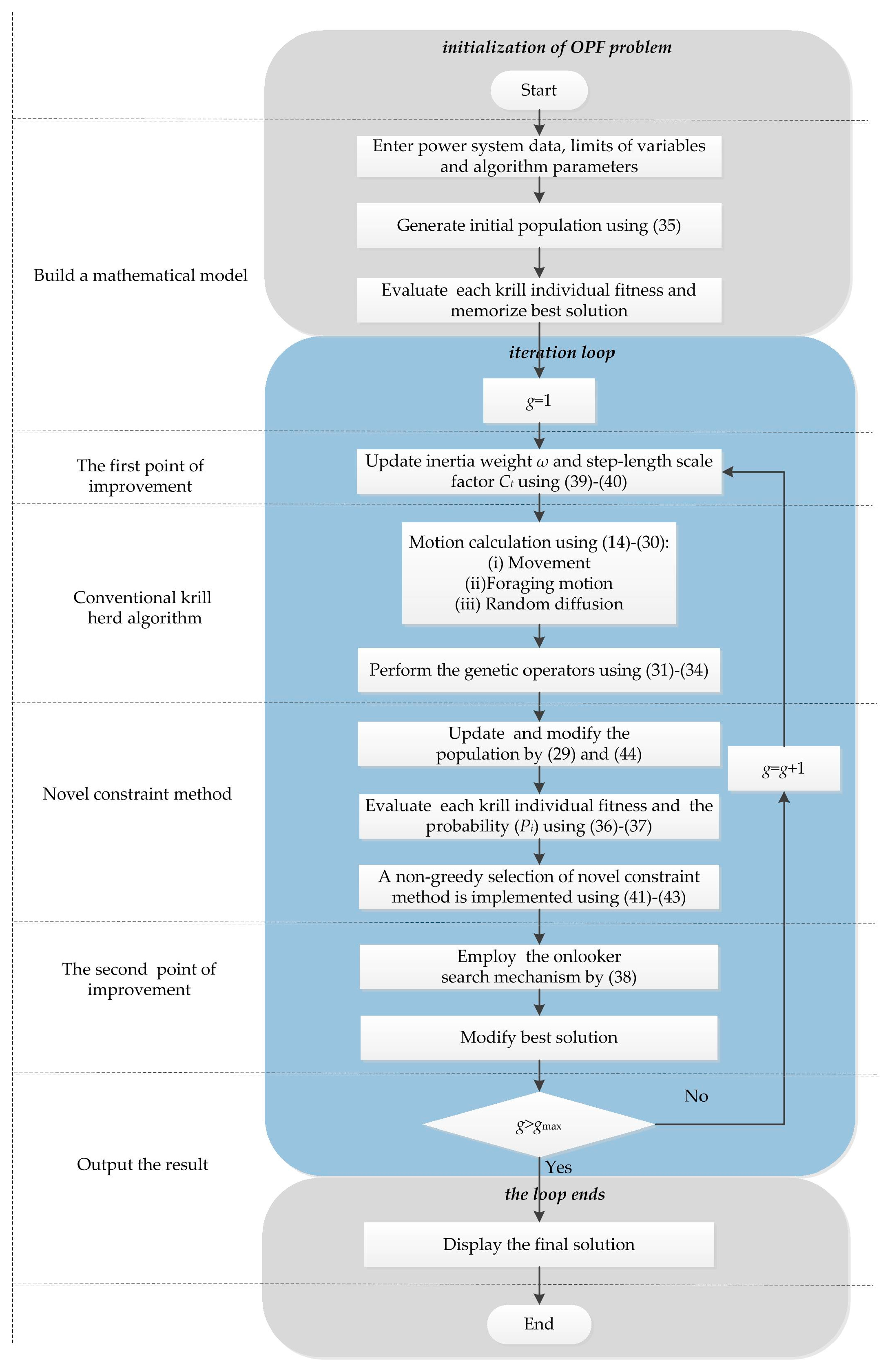
Some steps involved to solve the OPF problem by IKHA algorithm are presented in the flowchart shown in Figure 1.

4. Novel Constraint Handling Method

The non-linear, non-convex constrained optimization problem can be solved by indirect and direct methods. The indirect method means that constraints are incorporated in an explicit manner and the direct method means that constrained optimization problem is converted into unconstrained optimization problem [26]. In this paper, an indirect method combined with a non-greedy selection is proposed, which is divided into two parts as follows.

4.1. State Variable Constraint

In this method, the inequality constraints of state variables which contain real power generation at slack bus P_G1, reactive power generation at PV buses Q_G, load bus voltage magnitude V_L and line loading S_l are considered as the conditions of selecting optimal individual and mathematically formulated as:

$$\begin{array}{c}\mathrm{Constraint}(X_i)=C_{\mathrm{V}}{\displaystyle \sum _{i=1}^{\mathrm{NL}}Cos(V_{\mathrm{L}i})}+C_{\mathrm{Q}}{\displaystyle \sum _{i=1}^{\mathrm{NG}}Cos(Q_{\mathrm{G}i})}\\ +C_{\mathrm{P}}Cos(P_{\mathrm{G}1})+C_{\mathrm{S}}{\displaystyle \sum _{i=1}^{\mathrm{NTL}}Cos(S_{\mathrm{l}i})}\end{array}$$

(41)

where Constraint(X_i) is the constraint evaluation value of X_i. C_V、 C_Q、 C_P and C_S are constraint coefficients of state variables, respectively. Cos(V_Li), Cos(Q_Gi), Cos(P_G1) and Cos(S_li) respect the constraint value of the state variable V_L, Q_G, P_G1, S_l at the current operating state X_i, and each one can be expressed as follows:

$$Cos(x_i)==\{\begin{array}{c}\left|x_{i\min }-x_i\right|\\ 0\hspace{0.17em}\hspace{0.17em}\hspace{0.17em}\\ \left|x_{i\max }-x_i\right|\end{array}\hspace{0.17em}\hspace{0.17em}\begin{array}{c}\hspace{0.17em}{x}_i<x_{i\min }\\ x_{i\min }\le x_i\le x_{i\max }\\ x_i>x_{i\max }\end{array}$$

(42)

where x_i represents ith state variable of V_L, Q_G, P_G1 and S_l. x_imin and x_imax are lower and upper bounds of the state variable, respectively. Constraint coefficients are usually 1, but in large systems, if some state variable is easy to violate constraints, the value of its corresponding constraint coefficient can be increased.

A non-greedy selection based on constraint evaluation value Constraint(X_i) is introduced to pick out qualified solutions, mathematically formulated as:

$$X_i=\{\begin{array}{c}\begin{array}{cc}{X}_1& \mathrm{Constraint}(X_1)=0,\hspace{0.17em}\mathrm{Constraint}(X_2)\ne 0\end{array}\\ \begin{array}{cc}{X}_2& \mathrm{Constraint}(X_2)=0,\hspace{0.17em}\mathrm{Constraint}(X_1)\ne 0\end{array}\\ \begin{array}{cc}\min (\mathrm{Constraint}(X_1),\hspace{0.17em}\mathrm{Constraint}(X_2))& otherwise\end{array}\end{array}$$

(43)

The selection is applied in the algorithm to guide the individual to the feasible space.

4.2. Control Variable Constraint

On the other hand, the control variable is self-constrained. When the independent variable violates limits then the position of it will be adjusted as follows:

$$X_j=\{\begin{array}{l}{r}_1\times X_{j,\max }+(1-r_1)\times X_{j,\mathrm{best}}\\ r_2\times X_{j,\min }+(1-r_2)\times X_{j,\mathrm{best}}\end{array}\hspace{1em}\begin{array}{l}if\hspace{0.17em}\hspace{0.17em}{X}_j>X_{j\max }\\ if\hspace{0.17em}\hspace{0.17em}{X}_j<X_{j,\min }\end{array}\hspace{1em}j=1,\dots ,D$$

(44)

where X_j,best is the corresponding variable of the best individual, r₁ and r₂ are uniformly distributed random variables between 0 and 1.

5. Application and Simulation Results

To verify the efficiency of the proposed algorithm, 3 different types of test system and 10 different cases are considered for simulation, which are summarized in

Table 1. Summary of the studied cases.

Test System	Name	Objective Function	Constraints
IEEE 30	Case 1	Quadratic fuel cost function	Equality/non-equality
	Case 1-a	Fuel cost function with multiple fuel sources	Equality/non-equality
	Case 1-b	Fuel cost function with valve point effect	Equality/non-equality
	Case 2	Voltage magnitude deviation	Equality/non-equality
	Case 3	Fuel cost emission	Equality/non-equality
	Case 4	Transmission real power losses	Equality/non-equality
	Case 5	Quadratic cost considering voltage deviation	Equality/non-equality
	Case 6	Quadratic cost considering power losses	Equality/non-equality
IEEE 57	Case 7	Quadratic fuel cost function	Equality/non-equality
	Case 8	Voltage magnitude deviation	Equality/non-equality
	Case 9	Quadratic cost considering voltage deviation	Equality/non-equality
IEEE 118	Case 10	Quadratic fuel cost function	Equality/non-equality

. For each case, 30 runs are conducted to get the solution quality. In addition,

Table 2. Parameter values of improved krill herd algorithm (IKHA) and krill herd algorithm (KHA).

Algorithm	NP	gmax	Nmax	Vf	Dmax	Ct
IKHA	30	500	0.01	0.02	0.005	0.4/0.7
KHA	30	500	0.01	0.02	0.005	0.4

shows some parameter values of IKHA and KHA. The choices of these values which are obtained from multiple experiments can make the method have better search efficiency.

The simulations were performed in Matlab 2014 on a 3.30 GHz personal computer with 8.00 GB for random access memory (RAM) and the optimization results obtained by IKHA are compared with the results of KHA and other methods presented in the recent literatures. All of constraint coefficients of the novel constraint method are set to be 1 in IEEE 30 bus system, but C_V and C_Q are set to be 500 in IEEE 57 bus and IEEE 118 bus systems. Besides, KHA employs the penalty function to handle the constraints on state variables, and all of the penalty factors are set to be 500.

5.1. IEEE 30 Bus System

The system has 6 generators, 41 branches, 9 shunt reactive compensations and 4 transformers, which also has 2.834 p.u. for the active power demand and 1.262 p.u. for the reactive power demand on base of 100 MVA. In addition, the detailed line date, the bus date and the cost coefficients are given in [27,28]. The transformer tap settings are divided into 20 discrete steps. The minimum and maximum limits are 0.9 p.u. and 1.1 p.u., and the step size is 0.01 p.u. The shunt reactive compensation is divided into 50 discrete steps with a step of 0.001 p.u.; and the lower and upper limits are 0.0 p.u. and 0.05 p.u., respectively. Furthermore, the voltage magnitudes of generator buses are assumed to vary in the range [0.95, 1.1] p.u., and the lower and upper limits of load buses are considered to be 0.95 p.u. and 1.05 p.u., respectively.

5.1.1. Case 1: Minimization of Quadratic Fuel Cost Function

The objective of the total fuel cost is widely used and it can be formulated by a quadratic curve as follows:

$$f_{\mathrm{Cost}}={\displaystyle \sum _{i=1}^{\mathrm{NG}}{f}_i(\$/h)}$$

(45)

$$f_i=a_i+b_i{P}_{\mathrm{G}i}+c_i{P}_{\mathrm{G}i}^2$$

(46)

where a_i, b_i and c_i are the cost coefficients of the ith generator.

In actual operation of power systems, the fuel cost of generators is affected by some factors. Therefore, two other general formulas for calculating the fuel cost are also considered in this paper: Case 1-a and Case 1-b.

Case 1-a considers the situation where the generators use multiple fuel sources like natural gas, oil and coal. The mathematical formulation of these generators is described as a set of piecewise quadratic cost functions for different fuel types, which can be defined as:

$$f_i=\{\begin{array}{ll}{a}_{i1}+b_{i1}{P}_{Gi}+c_{i1}{P}_{Gi}^2& P_{\mathrm{G}i\min }^{}\le P_{\mathrm{G}i}<P_{\mathrm{G}i1}\\ a_{i2}+b_{i2}{P}_{Gi}+c_{i2}{P}_{Gi}^2& P_{\mathrm{G}i1}^{}\le P_{\mathrm{G}i}<P_{\mathrm{G}i2}\\ \dots & \\ a_{ik}+b_{ik}{P}_{Gi}+c_{ik}{P}_{Gi}^2& P_{\mathrm{G}ik-1}^{}\le P_{\mathrm{G}i}<P_{\mathrm{G}i\max }^{}\end{array}$$

(47)

where a_ik, b_ik and c_ik are the cost coefficients of the ith generator for fuel type k. In this case, the generators at buses 1 and 2 have two different types of fuel cost sources, and their cost coefficients are presented in [12]. The cost functions of other generators have the same presentations as Case 1. Clearly, the problem becomes non-continuous which may result in local optimum and the total objective function can be described as:

$$f_{\mathrm{Cost}-a}=\left({\displaystyle \sum _{i=1}^2{a}_{ik}+b_{ik}{P}_{\mathrm{G}i}+c_{ik}{P}_{\mathrm{G}i}^2}\right)+\left({\displaystyle \sum _{i=3}^{\mathrm{NG}}{a}_i+b_i{P}_{\mathrm{G}i}+c_i{P}_{\mathrm{G}i}^2}\right)(\$/h)$$

(48)

Case 1-b considers the valve point effect which is described as an absolute sinusoidal function [29]. In this case, the valve point effect is added to the basic quadratic cost functions of generators at buses 1 and 2, and the non-differential objective function is calculated as follows:

$$\begin{array}{c}{f}_{\mathrm{Cost}-b}=\left({\displaystyle \sum _{i=1}^2{a}_i+b_i{P}_{\mathrm{G}i}+c_i{P}_{\mathrm{G}i}^2+\left|d_i\sin \left(e_i\left(P_{\mathrm{G}i\min }^{}-P_{\mathrm{G}i}\right)\right)\right|}\right)\\ +\left({\displaystyle \sum _{i=3}^{\mathrm{NG}}{a}_i+b_i{P}_{\mathrm{G}i}+c_i{P}_{\mathrm{G}i}^2}\right) (\$/h)\end{array}$$

(49)

where a_i, b_i, c_i, d_i and e_i are cost coefficients of the ith generator, and the cost coefficients of buses 1 and 2 are given in [23]. The cost coefficients of other generators remain the same values as Case 1.

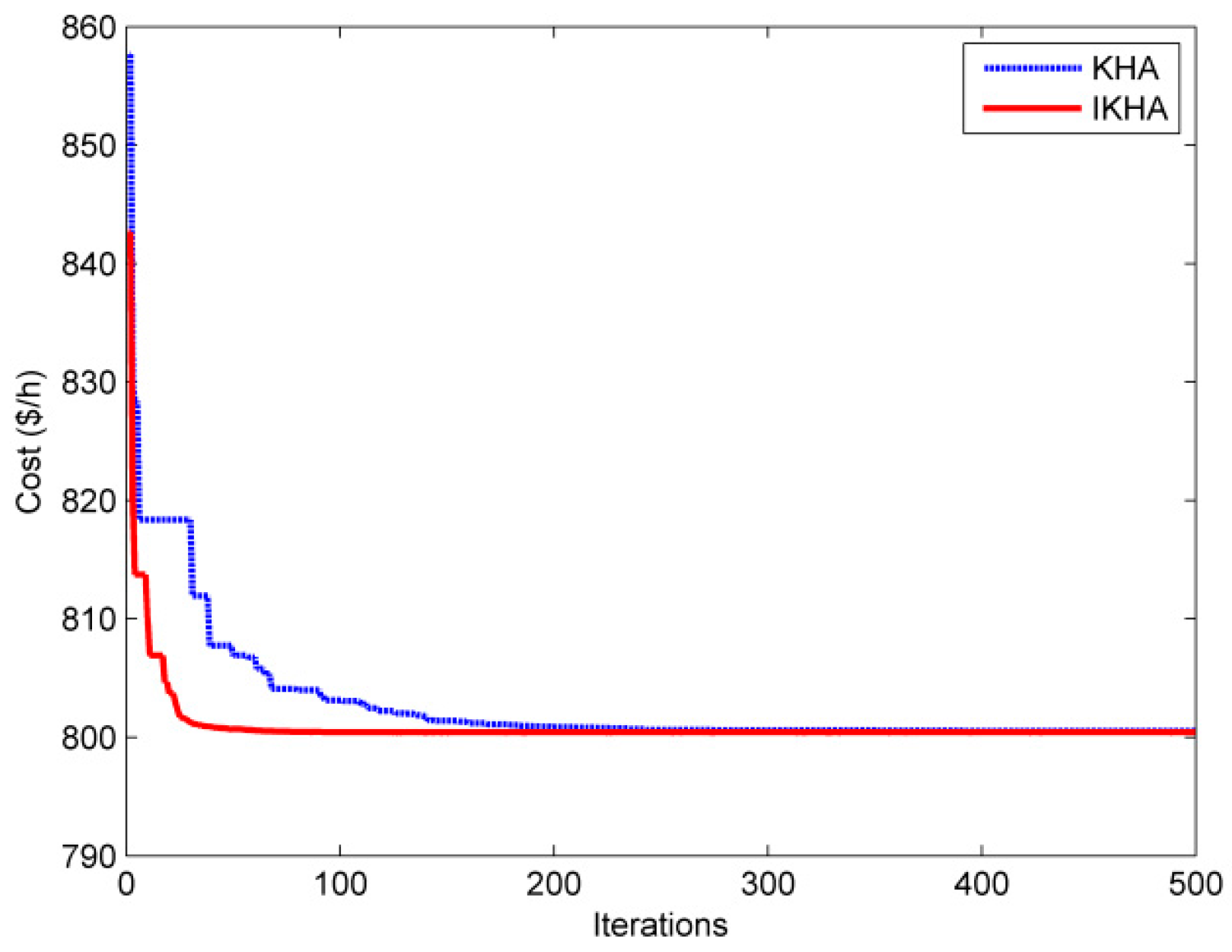
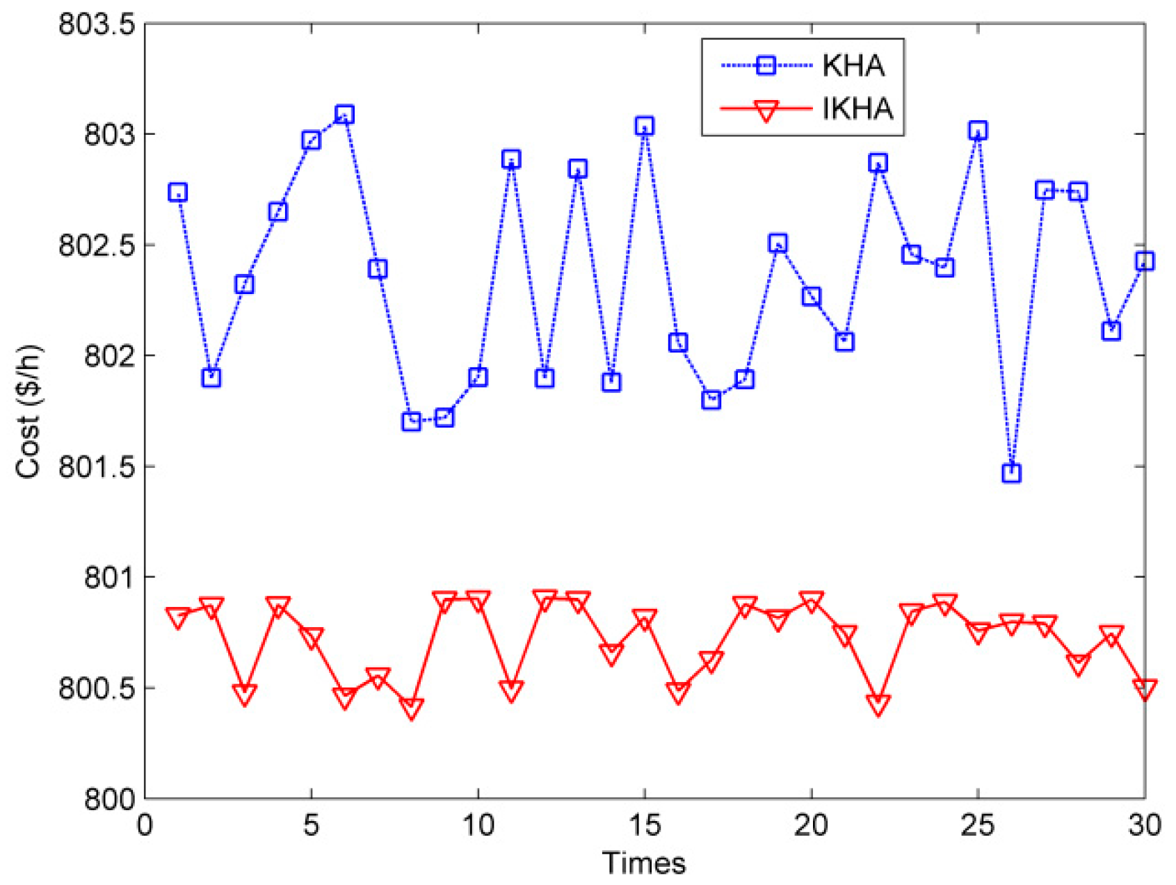
For Case 1, the optimal control variables and objective function value of IKHA are shown in

Table 3. Optimal solutions obtained by IKHA on IEEE 30 system.

Control Variables	Case 1	Case 1-a	Case 1-b	Case 2	Case 3	Case 4	Case 5	Case 6
P1 (MW)	177.0460	139.9931	199.2307	53.7862	64.0580	51.4880	176.4745	102.5066
P2 (MW)	48.7423	54.9987	51.9824	79.8421	67.5612	79.9973	48.8341	55.6717
P5 (MW)	21.3782	24.1051	15.0001	49.8070	50.0000	50.0000	21.6357	38.0835
P8 (MW)	21.3084	34.9883	10.0001	34.7705	35.0000	35.0000	22.0723	34.9998
P11 (MW)	11.9203	18.4108	10.0002	30.0000	30.0000	29.9998	12.2127	29.9980
P13 (MW)	12.0020	17.6480	12.0002	39.0733	40.0000	40.0000	12.0005	26.6695
V1 (p.u.)	1.0827	1.0734	0.9784	1.0054	1.0636	1.0609	1.0409	1.0675
V2 (p.u.)	1.0635	1.0593	0.9607	1.0070	1.0575	1.0569	1.0244	1.0571
V5 (p.u.)	1.0325	1.0341	0.9799	1.0189	1.0381	1.0377	1.0127	1.0338
V8 (p.u.)	1.0374	1.0401	0.9631	1.0114	1.0444	1.0441	1.0010	1.0421
V11 (p.u.)	1.0897	1.0972	1.0992	0.9880	1.0877	1.0805	1.0428	1.0773
V13 (p.u.)	1.0470	1.0411	0.9831	1.0049	1.0487	1.0564	0.9920	1.0511
T11 (p.u.)	1.0400	1.0300	0.9000	1.0000	1.0800	1.0800	1.0600	1.0500
T12 (p.u.)	0.9300	0.9800	0.9000	0.9000	0.9000	0.9000	0.9000	0.9100
T15 (p.u.)	0.9700	0.9700	1.1000	0.9700	0.9800	0.9900	0.9500	0.9900
T36 (p.u.)	0.9700	0.9700	0.9200	0.9500	0.9700	0.9800	0.9600	0.9800
QC10 (p.u.)	0.0020	0.0440	0.0480	0.0500	0.0000	0.0060	0.0500	0.0010
QC12 (p.u.)	0.0130	0.0440	0.0430	0.0000	0.0070	0.0000	0.0130	0.0430
QC15 (p.u.)	0.0410	0.0460	0.0050	0.0500	0.0440	0.0430	0.0500	0.0460
QC17 (p.u.)	0.0500	0.0350	0.0450	0.0000	0.0500	0.0500	0.0000	0.0500
QC20 (p.u.)	0.0390	0.0400	0.0120	0.0500	0.0390	0.0400	0.0500	0.0390
QC21 (p.u.)	0.0500	0.0460	0.0000	0.0500	0.0500	0.0500	0.0500	0.0500
QC23 (p.u.)	0.0280	0.0410	0.0470	0.0500	0.0280	0.0290	0.0500	0.0280
QC24 (p.u.)	0.0500	0.0480	0.0100	0.0500	0.0500	0.0500	0.0500	0.0500
QC29 (p.u.)	0.0220	0.0190	0.0040	0.0070	0.0190	0.0240	0.0170	0.0260
Fuel cost	800.4143	646.5126	929.901	965.5317	944.3314	967.6201	803.5879	859.0579
Voltage deviations	0.9215	0.9256	0.6826	0.0892	0.9226	0.8814	0.0984	0.9083
Emission	0.3660	0.2835	0.4410	0.2077	0.204818	0.2073	0.3642	0.2287
Power loss	8.9972	6.7439	14.8136	3.8792	3.2192	3.0850	9.8297	4.5291

, and the comparison of the results obtained by IKHA and other methods reported in recent literatures is shown in

Table 4. Comparison of the simulation results for Case 1 on IEEE 30 system.

Algorithms	Min ($/h)	Simulation Time (s)/gmax
IKHA	800.4143	75.11/500
KHA	801.4675	74.06/500
MSLFA [30]	802.2870	NA/100
ABC [31]	800.6600	130.16/200
MSA [22]	800.5099	NA/100
MGBICA [32]	801.1409	NA/NA
ARCBBO [34]	800.5159	NA/200
Jaya [33]	800.479	72.4/100
GSA [35]	798.6751 a	10.7582/200
BBO [36]	799.1116 a	NA/200

^a Infeasible solution.

. The computation time is a vital issue in power system operation which depends on the algorithm’s search efficiency, maximum iteration number and population size. In recent literatures, the maximum iteration number and population size which are related to time complexity are usually not the same. The average computation time of the single iteration is considered to reflect the algorithm efficiency in this paper. Thus, the simulation time and maximum iteration number of methods are recorded which can be seen in Table 4. It is worth noting that the result with ‘^a’ represents an infeasible solution. NA means that the datum is not reported in the referred literature. From the tables, it is clear that the minimization of quadratic fuel cost obtained by IKHA is better than KHA, modified shuffle frog leaping algorithm (MSLFA) [30], ABC [31], moth swarm algorithm (MSA) [22], modified Gaussian bare-bones imperialist competitive algorithm (MGBICA) [32], Jaya [33] and adaptive real coded biogeography-based optimization (ARCBBO) [34]. The single iteration computation times of ABC [31] and Jaya [33] are longer than IKHA, which shows the search efficiency of IKHA. The result of IKHA is greatly reduced to 800.4143 $/h comparing with 801.4675 $/h obtained by KHA, and the difference of the simulation time is small which proves the effectiveness of the proposed method. Although the results obtained by GSA [35] and biogeography based optimization (BBO) [36] are less than IKHA, the optimal solutions are regarded as unqualified solutions for violating system security constraints mentioned before. Meanwhile, Figure 2 shows the optimal convergence curves over the iterations and Figure 3 shows the results in 30 independent simulations of IKHA and KH for case 1. As shown in Figure 2, the initial value of IKHA is smaller than KHA due to the novel constraint method; and IKHA has smooth curve with a better convergence than KHA. Moreover, the distribution range of results of IKHA is smaller than KHA according to Figure 3, which demonstrates that IKHA has a stronger robustness.

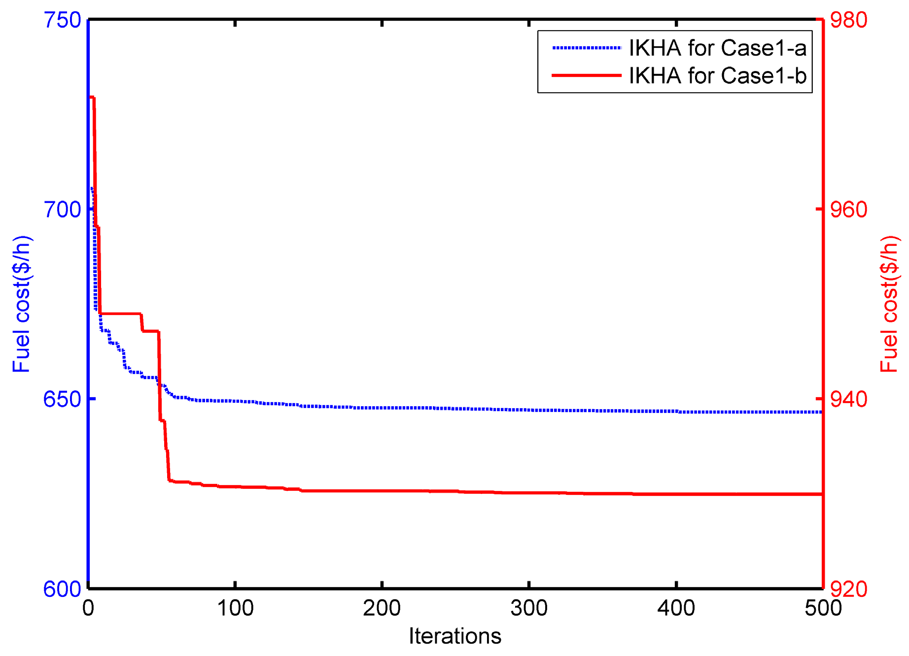
For Case 1-a and Case 1-b, the optimal control variables and objective function values of IKHA are shown in Table 3, and the comparison of the results is shown in

Table 5. Comparison of the simulation results for Case 1-a and Case 1-b on IEEE 30 system.

Algorithms	Case 1-a Min ($/h)	Case 1-b Min ($/h)	Average Time (s)/gmax
IKHA	646.5126	929.9010	80.75/500
KHA	647.0264	932.1784	78.22/500
MSA [22]	646.8364	930.7441	NA/100

. It can be seen that the results of IKHA are 646.5126 $/h and 929.9010 $/h for Case 1-a and Case 1-b, which are both less than KHA and MSA [22]. Furthermore, the optimal convergence curves of IKHA for Case 1-a and Case 1-b are shown in Figure 4 which demonstrates the convergence characteristic. According to the experimental data of the three situations, the proposed method can successfully solve the non-differential and non-continuous OPF problem which contains the discrete and continuous variables.

5.1.2. Case 2: Minimization of Voltage Magnitude Deviation

The function which is an important safety quality index aims to minimize the deviation of the PQ buses voltages from 1.0, and it can be formulated as follows:

$$f_{\mathrm{Deviation}}={\displaystyle \sum _{i=1}^{\mathrm{NL}}|V_i-1|}$$

(50)

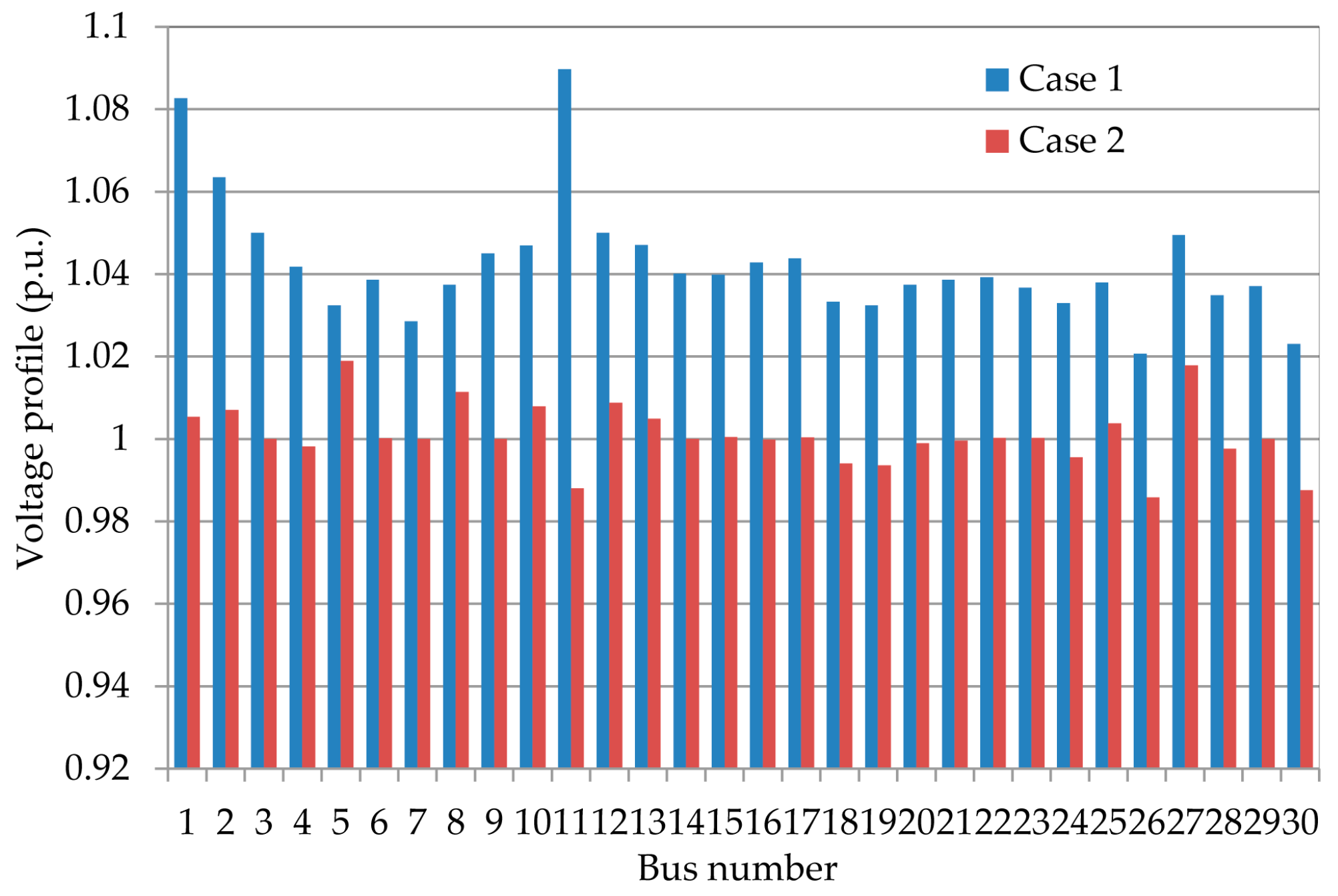
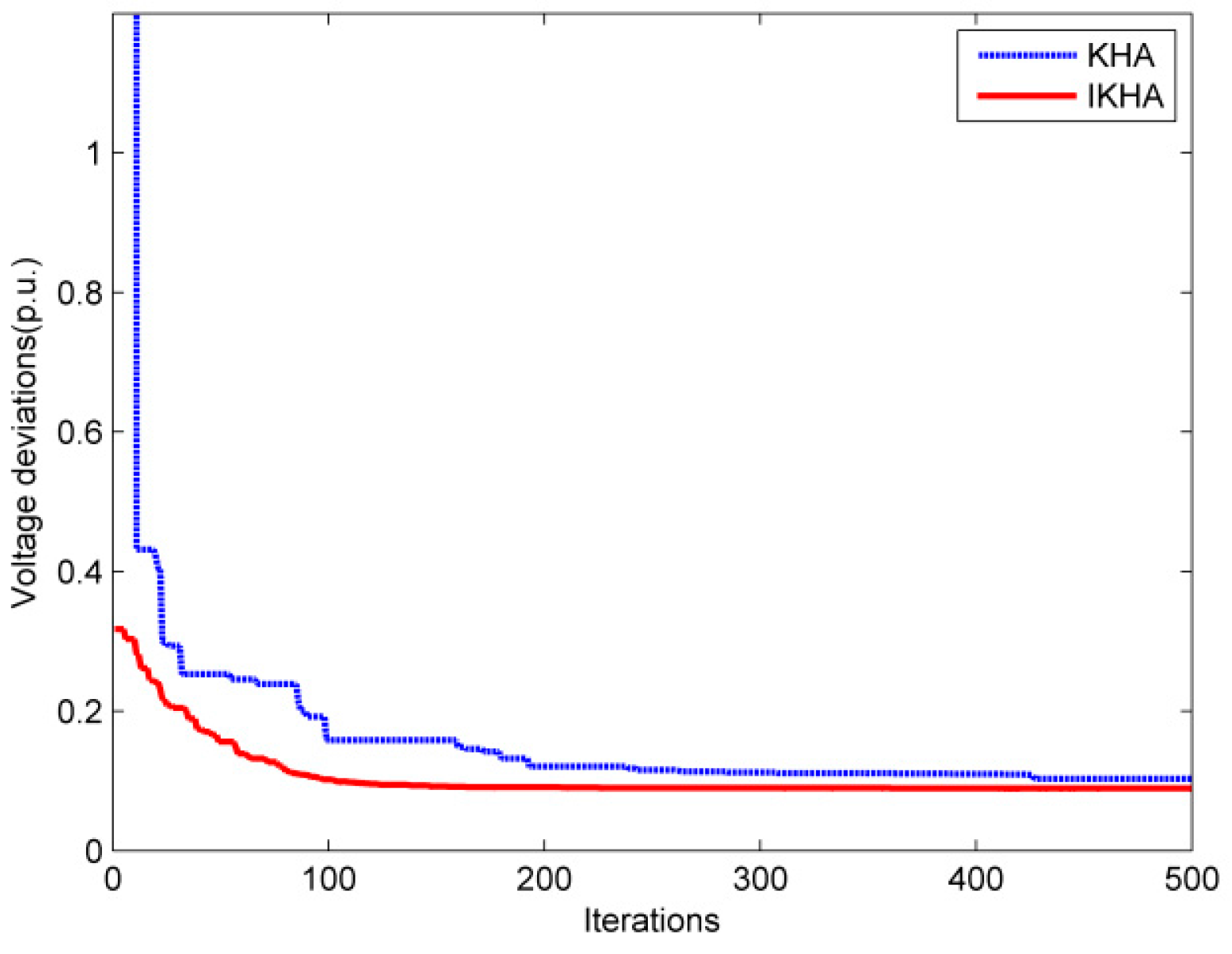
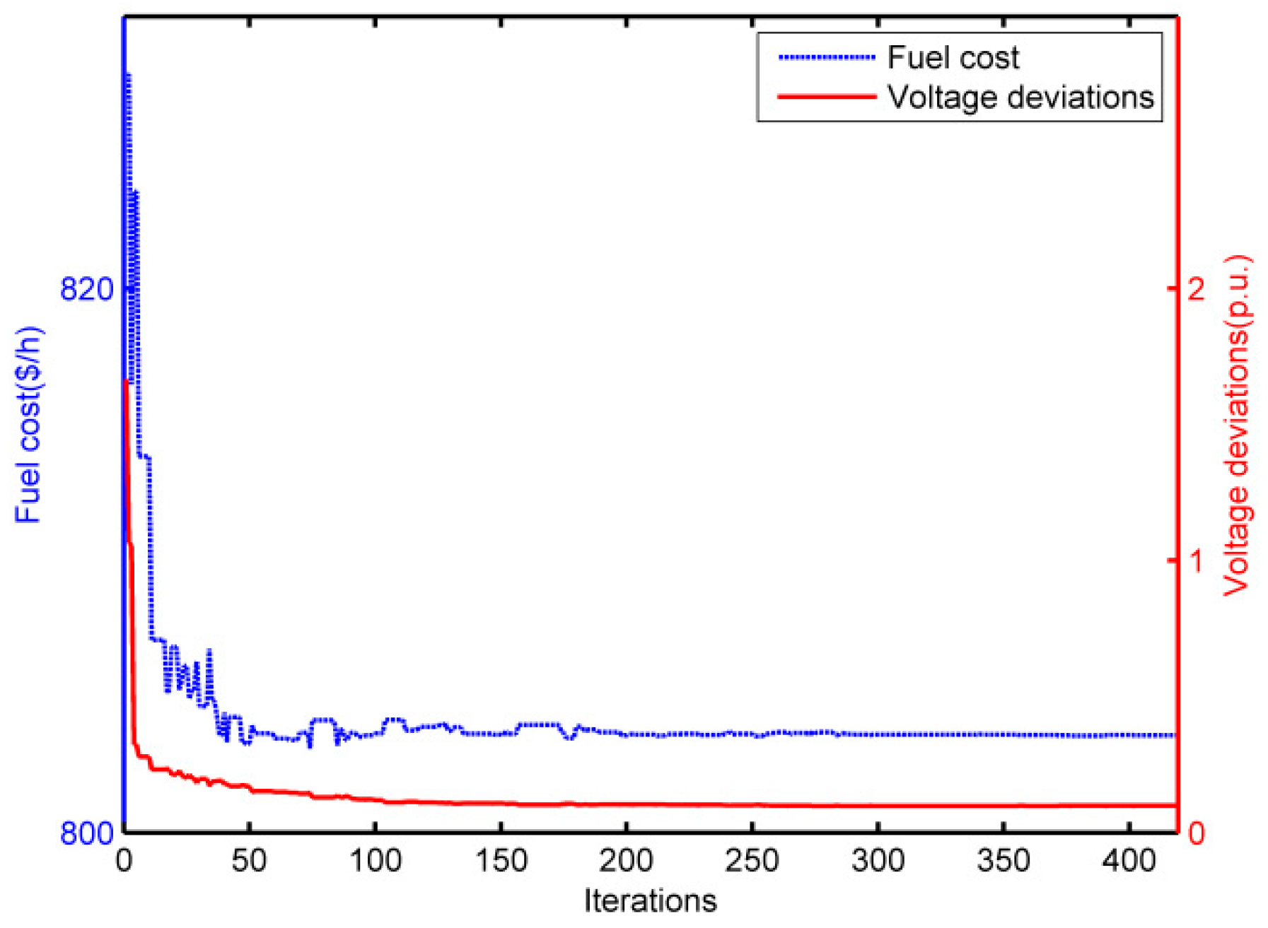
where NL is the number of load buses and V_i represents the voltage magnitude of ith load bus. For case 2, Table 3 shows the optimal solutions of IKHA and

Table 6. Comparison of the simulation results for Case 2 on IEEE 30 system.

Algorithms	Min	Simulation Time (s)/gmax
IKHA	0.0892	70.40/500
KHA	0.1029	68.02/500
MGBICA [32]	0.1239	NA/NA
LTLBO [23]	0.0974	20.17/100
BBO [36]	0.0951	NA/200

shows the comparison of the results obtained by IKHA and other methods. It can be seen that the minimization of voltage magnitude deviation of IKHA is 0.0892 p.u., which is less by 0.0137, 0.0347, 0.0082 and 0.0059 p.u. comparing with KHA, MGBICA [32], lévy teaching–learning-based optimization (LTLBO) [23] and BBO [36], respectively. Moreover, the voltage magnitude deviation in this case is decreasing from 0.9215 p.u. obtained by case 1 to 0.0892 p.u., which is equivalent to 90% reduction. In order to make the result of case 2 clearer, the comparison of voltage profiles between case1 and case 2 is shown in Figure 5, and the optimal convergence curves of IKHA and KH is shown in Figure 6. It is noted that the initial value of KHA is not shown in Figure 6 for making the convergence curve better clear. The reason for this is that the difference between the initial values of IKHA and KHA is larger due to the difference of the novel constraint method and the penalty function method. Obviously, the proposed method can guide the individual to find the better location in the viable domain.

5.1.3. Case 3: Minimization of Fuel Cost Emission

Aimed to minimize the harmful gas amount, such as SO_x and NO_x, the objective for the generators can be defined as bellow [37]:

$$f_{\mathrm{E}}={\displaystyle \sum _{i=1}^{\mathrm{NG}}{\alpha }_i+{\beta }_i{P}_{\mathrm{G}i}+}{\gamma }_i{P}_{\mathrm{G}i}^2+{\xi }_i\exp ({\lambda }_i{P}_{\mathrm{G}i})\hspace{0.17em}\mathrm{ton}/\mathrm{h}$$

(51)

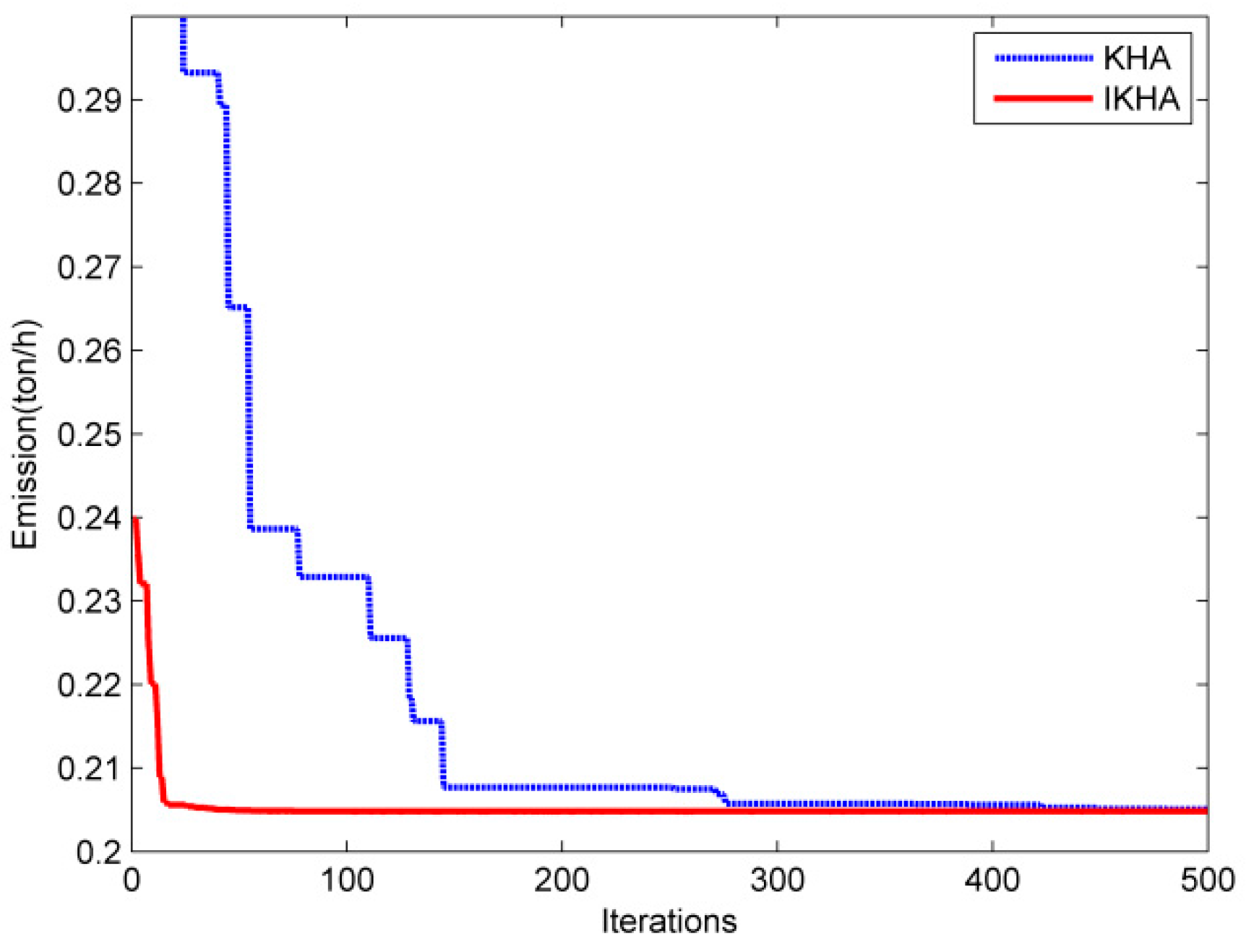
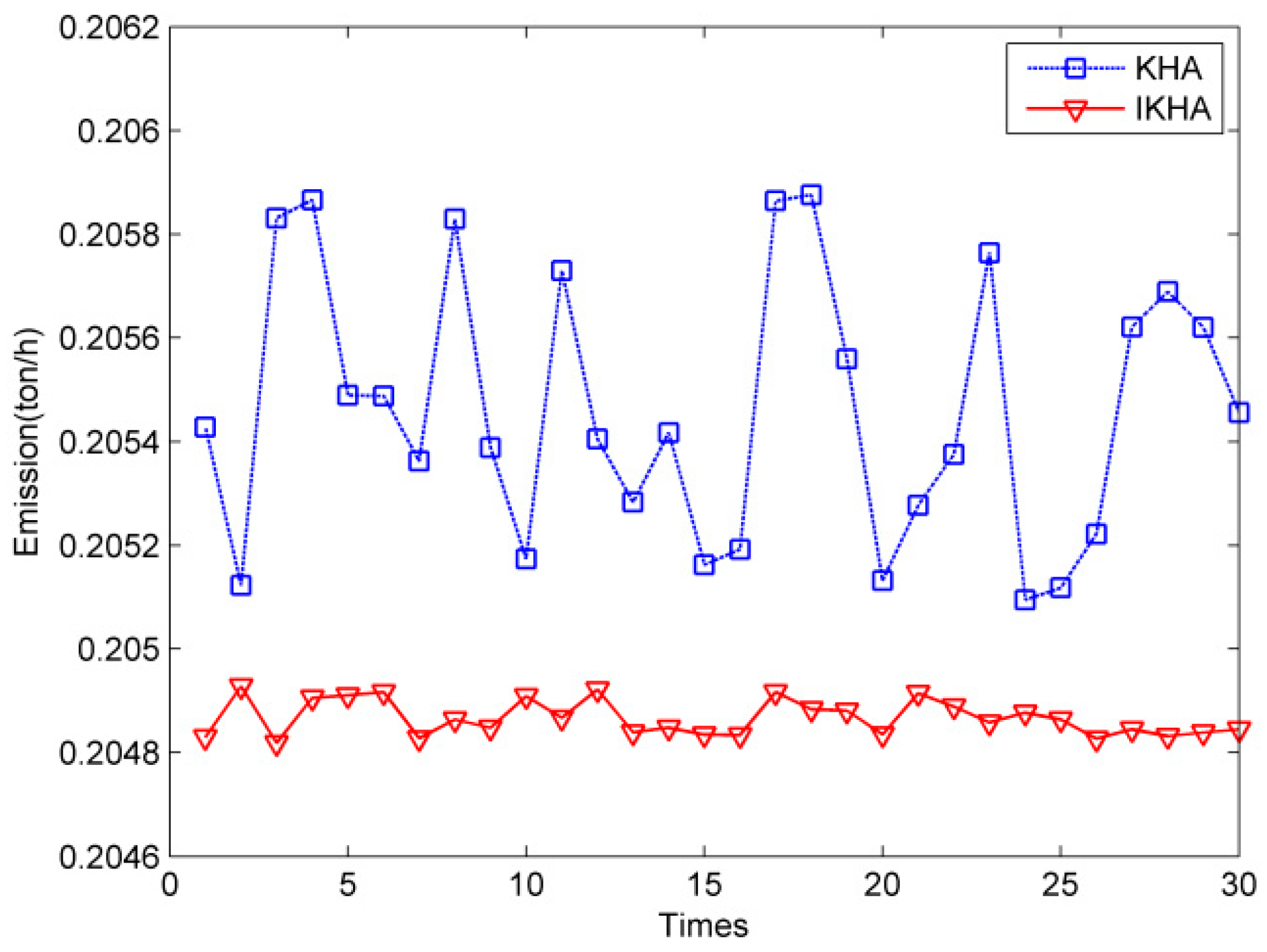
where α_i, β_i, γ_i, ξ_i and λ_i are the emission coefficients of the ith generator. NG represents the number of generator buses. The setting of optimal control variables of IKHA are presented in Table 3, which shows that the minimum of fuel cost emission obtained by IKHA is 0.204818 ton/h. The simulation result is compared with other methods in

Table 7. Comparison of the simulation results for Case 3 on IEEE 30 system.

Algorithms	Min (ton/h)	Simulation Time (s)/gmax
IKHA	0.204818	76.68/500
KHA	0.205082	74.89/500
DSA [9]	0.2058255	NA/500
ABC [31]	0.204826	NA/200
MSA [22]	0.20482	NA/100
MGBICA [32]	0.2048	NA/NA
MSLFA [30]	0.2056	NA/100

, and better than KHA, differential search algorithm (DSA) [9] ABC [31], MSA [22], MGBICA [32] and MSLFA [30]. Compared with the above cases, this objective function is non-linear. The result of IKHA, which is less 0.001002 than KHA, proves that the proposed method can get not only the better optimal solution but also better convergence curve when solving non-linear problem as shown in Figure 7. Besides, Figure 8 shows the results in 30 independent simulations of IKHA and KH for case 3, which indicates the robustness of IKHA.

5.1.4. Case 4: Minimization of Transmission Real Power Losses

The function determined by the bus voltage magnitude and angle is the total active power losses of all transmission lines, and can be formulated as follows:

$$f_{\mathrm{Loss}}={\displaystyle \sum _{k=1}^{\mathrm{NTL}}{G}_k[V_i{}^2+V_j{}^2-2V_i{V}_j\cos ({\delta }_i-{\delta }_j)]}$$

(52)

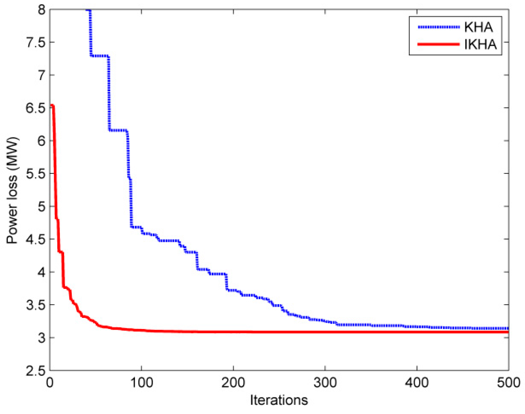
where G_k is the conductance between bus i and bus j, and NTL is the number of transmission lines. It can be seen in Table 3 that the minimization of transmission real power losses obtained by IKHA is 3.0850 MW, and the result is less than KHA, ABC [31] Combined approach [28], DSA [9] MSA [22], MGBICA [32], Proposed efficient evolutionary algorithm (EEA) [38], Jaya [33] and ALC-PSO [13] reported in

Table 8. Comparison of the simulation results for Case 4 on IEEE 30 system.

Algorithms	Min (MW)	Simulation Time (s)/gmax
IKHA	3.0805	72.32/500
KHA	3.1409	70.64/500
ABC [31]	3.1078	NA/200
Combined approach [28]	3.2601	3.3109/NA
DSA [9]	3.0945	NA/500
MSA [22]	3.1005	NA/100
MGBICA [32]	4.937	NA/NA
Proposed EEA [38]	3.2823	5.7167/94
ALC-PSO [13]	3.1700	10.2345/500
Jaya [33]	3.1035	NA/100

. But the single iteration computation times of Proposed EEA [38] and ALC-PSO [13] are shorter than IKHA. As shown in Figure 9 and Figure 10, to a certain extent, the onlooker search mechanism reduces the probability of falling into the local optimal and makes the IKHA obtain a better solution compared with the basic KHA.

5.1.5. Case 5: Minimization of Quadratic Cost and Voltage Magnitude Deviation

Generally, the weighted sum method is used to make multi-objective into a single objective problem. This case is aimed to simultaneously minimize the quadratic cost and voltage magnitude deviation, which can be expressed as:

$$f_{\mathrm{CD}}=f_{\mathrm{Cost}}+{\lambda }_{\mathrm{D}}{f}_{\mathrm{Deviation}}$$

(53)

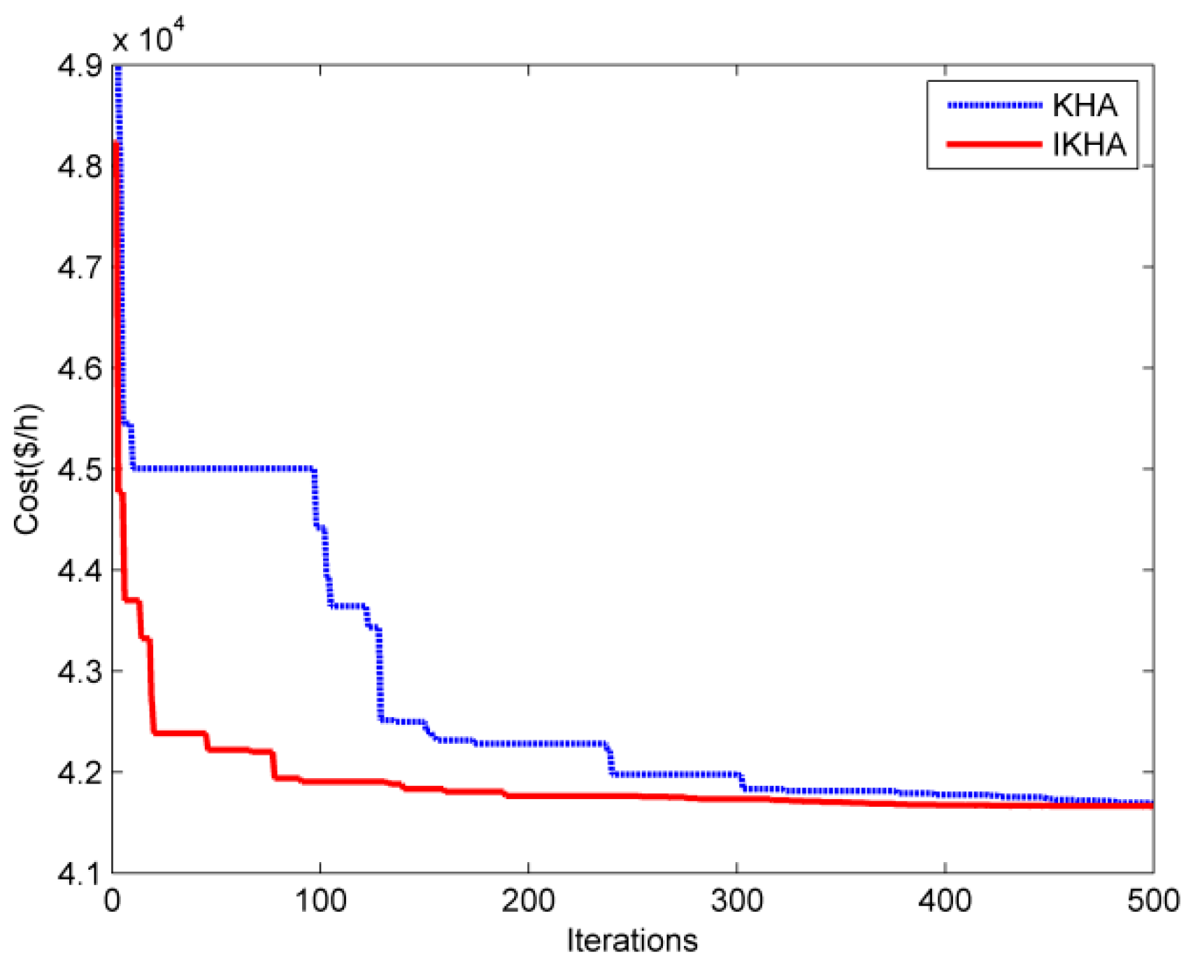
where λ_D selected by the user is a weighting factor and it is selected as 100 in this study [23]. Table 3 shows that the quadratic fuel cost and voltage magnitude deviation for case 5 of IKHA are 803.5879 $/h and 0.0984 p.u, respectively. It is also shows 0.3965% increase in the quadratic fuel cost and 89.32% reduction in the voltage magnitude deviation compared with case 1. Additionally, the results are compared with other methods, and the comparison is shown in

Table 9. Comparison of the simulation results for Case 5 on IEEE 30 system.

Algorithms	Fuel Cost ($/h)	Voltage Deviations	Total	Time (s)/gmax
IKHA	803.5879	0.0984	813.4279	78.36/500
KHA	803.8889	0.0987	813.7589	75.68/500
PSOGSA [29]	804.43123	0.09638	814.06923	NA/200
The proposed KHA [39]	804.6337	0.0996	814.5937	NA/100
ABPPO [40]	804.7339	0.09232	813.9659	NA/300
MSA [22]	803.3125	0.10842	814.1545	NA/100
LTLBO [23]	803.7431	0.0974	813.4831	20.17/100
GABC [24]	803.5785	0.1007	813.6485	2.98/100
ICBO [12]	803.3978	0.1014	813.5378	NA/500

. According to the value of the weighted sum, IKHA is better than KHA, particle swarm optimization and gravitational search algorithm (PSOGSA) [29], The proposed KHA [39], adaptive biogeography based predator–prey optimization (ABPPO) [40], MSA [22], LTLBO [23], Gbest guided artificial bee colony algorithm (GABC) [24] and ICBO [12] Looking at the two goals separately, the results of IKHA are lower than those of KHA and the proposed KHA For the results of the other methods in Table 8, such as the PSOGSA [29], only one of the two goals is better than IKHA. As the individual evaluation criteria are different, the optimal solution is different. The optimal convergence curves of quadratic fuel cost and voltage magnitude deviation of IKHA are shown in The Figure 11.

5.1.6. Case 6: Minimization of Quadratic Cost and Transmission Real Power Losses

Similarly, this case minimizes the quadratic cost and transmission real power losses at the same time through the weighted sum method, which is calculated as:

$$f_{\mathrm{CL}}=f_{\mathrm{Cost}}+{\lambda }_{\mathrm{L}}{f}_{\mathrm{Loss}}$$

(54)

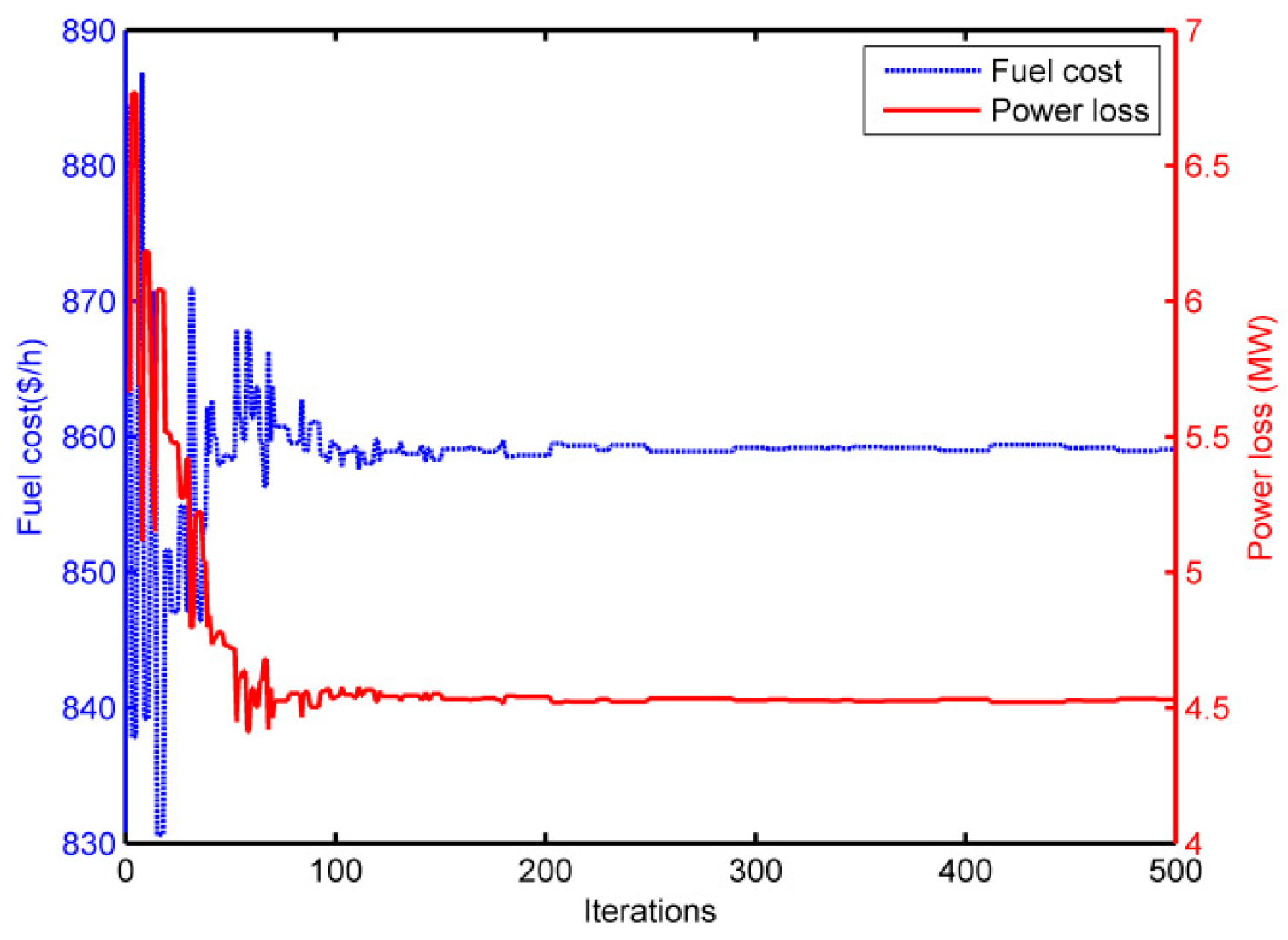
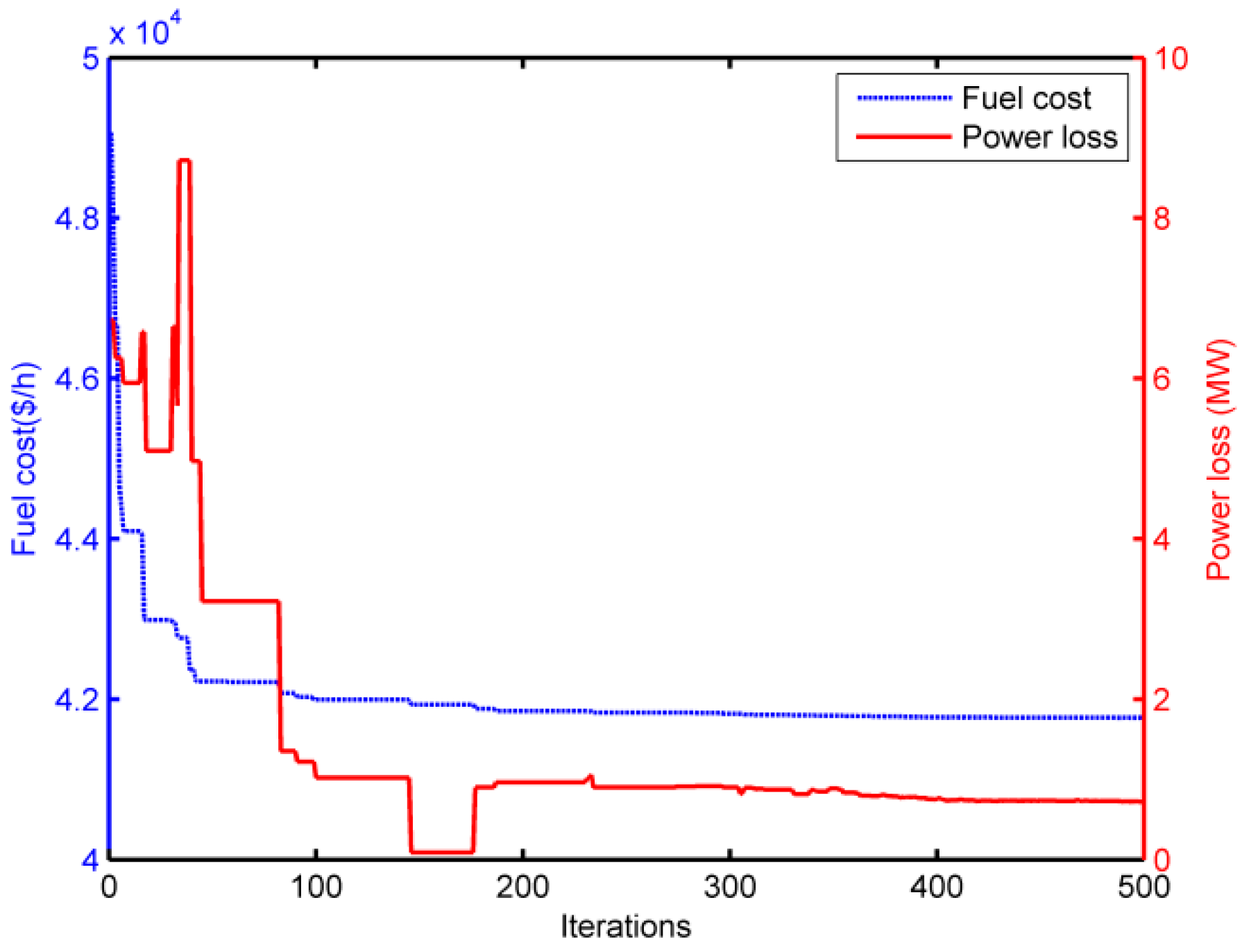
where λ_L selected by the user is a weighting factor and it is selected as 40 in this study [22]. From Table 3, the quadratic fuel cost and transmission real power losses for case 6 obtained by IKHA are 859.0579 $/h and 4.5291 MW, respectively. It is also shows 7.3266% increase in the quadratic fuel cost and 49.661% reduction in the transmission real power losses compared with case 1. The simulation results are compared with other methods in

Table 10. Comparison of the simulation results for Case 6 on IEEE 30 system.

Algorithms	Fuel Cost ($/h)	Power Loss (MW)	Total	Simulation Time (s)/gmax
IKHA	859.0579	4.5291	1040.2219	77.29/500
KHA	859.4961	4.5246	1040.4801	75.04/500
MSA [22]	859.1915	4.5404	1040.8075	NA/100
MDE [22]	868.7138	4.3891	1044.2778	NA/100
PSOGSA [29]	822.40631	5.46816	1041.13271	NA/200
ABPPO [40]	822.7693	5.452	1040.8493	NA/300

, and the value of the weighted sum is better than KHA, MSA [22], modified differential evolution (MDE) [22], PSOGSA [29] and ABPPO [40]. The analysis of current case is similar to Case 5 because that the different criteria make different choices. The Figure 12 shows the optimal convergence curves of quadratic fuel cost and transmission real power losses over the iterations, which is very different from Figure 11 due to the differences between nonlinear and linear objective functions. This case proves that IKHA can handle the OPF problem successfully.

5.2. IEEE 57 Bus System

The system has seven generators, three shunt reactive compensations and 15 transformers, which also has 12.508 p.u. for the active power demand and 3.364 p.u. for the reactive power demand on base of 100 MVA. All detailed line date, the bus date and the cost coefficients are given in [41]. The transformer tap settings are divided into 2000 discrete steps. The minimum and maximum limits are 0.9 p.u. and 1.1 p.u., and the step size is 0.0001 p.u. The shunt reactive compensation is divided into 3000 discrete steps with a step of 0.0001 p.u.; and the lower and upper limits are 0.0 p.u. and 0.3 p.u., respectively. Furthermore, the voltage magnitudes of generator buses are assumed to vary in the range [0.9, 1.1] p.u. and the lower and upper limits of load buses are considered to be 0.94 p.u. and 1.06 p.u., respectively.

5.2.1. Case 7: Minimization of Quadratic Fuel Cost Function

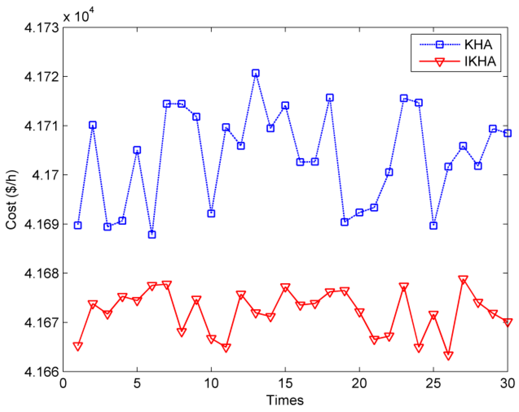
The objective function in this case is the minimization of quadratic cost which is given by Equations (45) and (46). The setting of optimal control variables for case 7 of IKHA are presented in

Table 11. Optimal solutions obtained on IEEE 57 system.

Control Variables	Case7	Case8	Case9
	IKHA	IKHA	IKHA	DSA [9]	MSA [22]
P1 (MW)	143.0334	355.4995	142.8777	142.6780	143.8661
P2 (MW)	85.3299	2.3831	88.5835	89.6450	85.34818
P3 (MW)	44.8387	124.4492	45.1741	45.6795	45.85493
P6 (MW)	75.1387	86.9520	70.3558	73.1394	71.30797
P8 (MW)	461.8476	212.7213	460.6468	461.7316	462.4092
P9 (MW)	95.0960	99.1914	96.7565	92.1106	94.08068
P12 (MW)	360.3747	387.2737	361.9443	361.4796	363.8543
V1 (p.u.)	1.0528	1.0082	1.0269	1.0212	1.022121
V2 (p.u.)	1.0494	1.0001	1.0246	1.0740	1.019646
V3 (p.u.)	1.0455	1.0125	1.0185	1.0646	1.013444
V6 (p.u.)	1.0581	1.0032	1.0313	0.9913	1.025691
V8 (p.u.)	1.0748	1.0086	1.0505	1.0519	1.044968
V9 (p.u.)	1.0587	1.0192	1.0312	1.0808	1.014033
V12 (p.u.)	1.0397	1.0232	1.0115	1.0103	1.010858
T4-18 (p.u.)	1.0449	0.9935	0.9690	0.9688	0.9101725
T4-18 (p.u.)	0.9495	0.9472	0.9901	0.9952	1.075124
T21-20 (p.u.)	1.0223	0.9765	0.9933	1.0248	0.9854176
T24-25 (p.u.)	0.9577	1.0504	0.9640	1.0010	0.9872317
T24-25 (p.u.)	1.0798	1.0465	1.0665	1.0025	1.053424
T24-26 (p.u.)	1.0190	0.9985	1.0179	0.9452	1.016568
T7-29 (p.u.)	0.9970	0.9985	1.0059	0.9000	1.00709
T34-32 (p.u.)	0.9672	0.9237	0.9405	0.9443	0.9348021
T11-41 (p.u.)	0.9028	0.9000	0.9005	0.9542	0.900021
T15-45 (p.u.)	0.9712	0.9317	0.9624	0.9772	0.9479471
T14-46 (p.u.)	0.9616	0.9740	0.9611	0.9252	0.9608689
T10-51 (p.u.)	0.9795	1.0097	0.9799	0.9665	0.9781408
T13-49 (p.u.)	0.9355	0.9013	0.9343	1.0116	0.9182851
T11-43 (p.u.)	0.9833	0.9648	0.9610	0.9343	0.9509346
T40-56 (p.u.)	0.9945	1.0188	1.0210	1.0130	0.9941227
T39-57 (p.u.)	0.9605	0.9010	0.9274	0.9861	0.9361633
T9-55 (p.u.)	1.0093	1.0186	1.0098	1.0214	0.998129
QC18 (p.u.)	0.1037	0.0025	0.0667	0.1095	0.1188253
QC25 (p.u.)	0.1437	0.1890	0.1648	0.1370	0.1678665
QC53 (p.u.)	0.1243	0.2889	0.1482	0.1326	0.1828455
Fuel cost ($/h)	41,663.3910	48,834.0293	41,697.5456	41,699.4	41,714.9851
V-deviatios	1.5494	0.5520	0.7233	0.7620	0.67818
Total	41,818.3310	48,889.22930	41,769.8815	41,775.6	41,782.8031

, which shows that the minimum of quadratic fuel cost obtained by IKHA is 41,663.391 $/h. The simulation result is compared with other methods in

Table 12. Comparison of the simulation results for Case 7 on IEEE 57 system.

Algorithms	Min ($/h)	Simulation Time (s)/gmax
IKHA	41,663.3910	136.34/500
KHA	41,687.8183	130.85/500
MSA [22]	41,673.7231	NA/NA
LTLBO [23]	41,679.5451	NA/150
ICBO [12]	41,697.3324	NA/1500
DSA [9]	41,686.82	NA/500
ARCBBO [34]	41,686	NA/500
GABC [42]	41,684.2011	NA/100

, and less than the results of KHA, MSA [22], LTLBO [23], ICBO [12], DSA [9], ARCBBO [34] and GABC [42]. Figure 13 shows the optimal convergence curves over the iterations and Figure 14 shows the results in 30 independent simulations of IKHA and KH for case 7. From Figure 13, it is clear that the convergence characteristic is not as good as case 1 in the same maximum iteration number, and the reason is that the system becomes bigger which means that the problem is more complicated. Besides, the initial value of KHA is also not shown in Figure 13 and the reason is described in case 2. Moreover, the distribution range of results of IKHA is smaller than KHA according to Figure 14, which demonstrates that IKHA also has a stronger robustness in larger systems.

5.2.2. Case 8: Minimization of Voltage Magnitude Deviation

The goal of this case is to minimize the voltage magnitude deviation which is given by Equation (50). The setting of optimal control variables of IKHA for case 8 are presented in Table 11. Apparently, the solution in this case is decreasing from 1.5494 p.u. obtained by case 7 to 0.552 p.u., which is equivalent to 64.3733% reduction. In order to make the result of case 8 clearer, the comparison of voltage profiles between case7 and case 8 is shown in Figure 15.

5.2.3. Case 9: Minimization of Quadratic Cost and Voltage Magnitude Deviation

In this case, the objective function is to minimize the quadratic cost and voltage magnitude deviation simultaneously, which is given by Equation (53). It can be seen in Table 11 that the quadratic fuel cost, voltage magnitude deviation and the value of the weighted sum are 41,697.5456 $/h, 0.7233 p.u. and 41,769.8815, respectively. And the results both are less than DSA [9].The optimal solution of MSA [22] shows 0.0418% increase in the quadratic fuel cost and 6.2381% reduction in the voltage magnitude deviation compared with IKHA. Additionally, the optimal convergence curves of quadratic fuel cost and voltage magnitude deviation over the iterations of IKHA for case 9 are shown in Figure 16.

5.3. IEEE 118 Bus System

The IEEE 118 bus system has 54 generators, 186 lines, nine transformers and 14 shunts reactive compensations which contain 2 reactors and 12 capacitors. The active and reactive power demands of the large system are 42.42 p.u and 14.39 p.u. on base of 100 MVA, respectively. Furthermore, the detailed data and cost coefficients of the system are taken form [41]. The transformer tap settings are divided into 200 discrete steps. The minimum and maximum limits are 0.9 p.u. and 1.1 p.u., and the step size is 0.001 p.u. The shunt reactive compensation is divided into different discrete steps and has different minimum and maximum limits which can be seen in [41]. The larger the system is, the harder the convergence of OPF problem will be. So, in this system, the maximum iteration number g_max is set as 1000.

Case 10: Minimization of Quadratic Fuel Cost Function

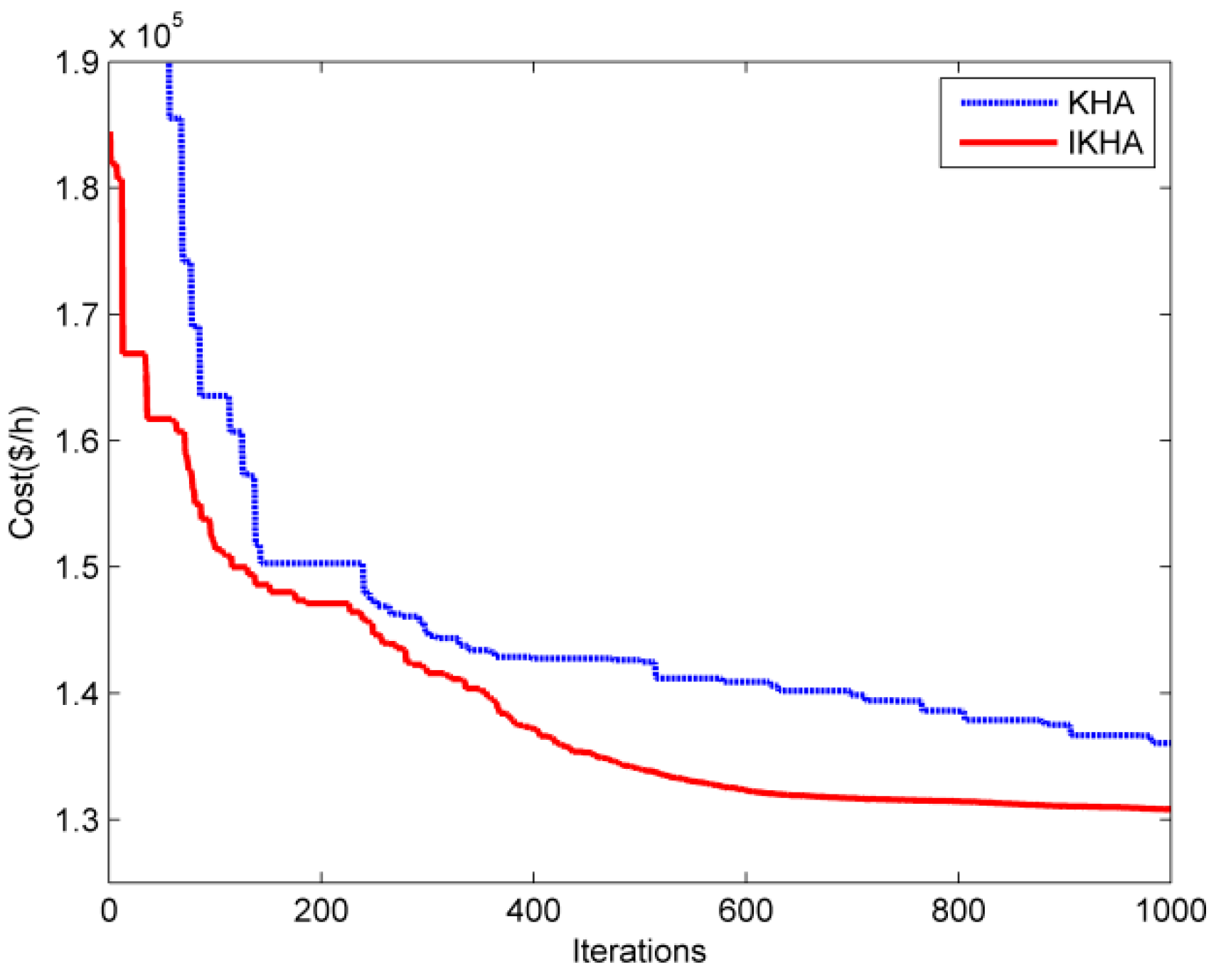
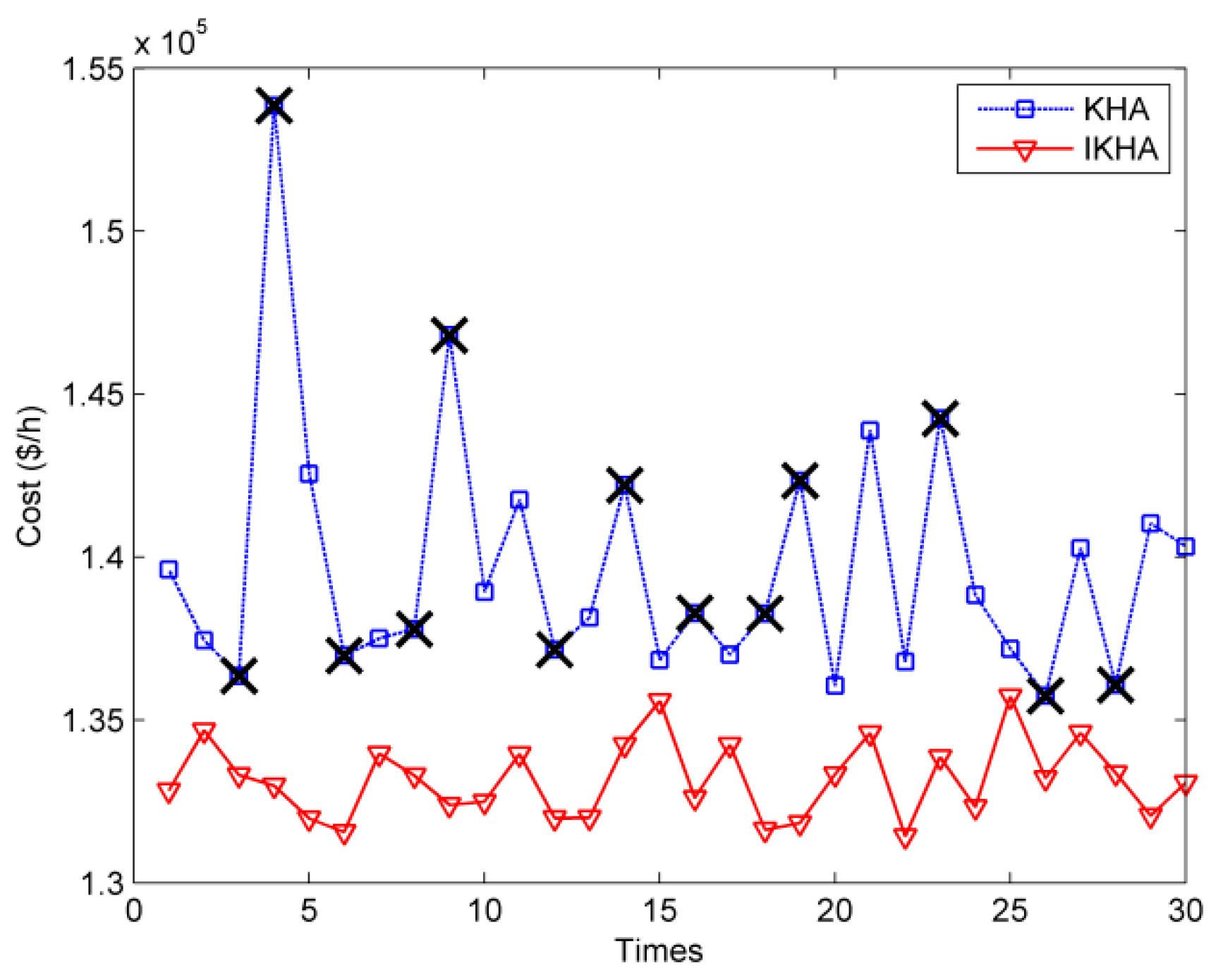
The objective function in this case is the minimization of quadratic fuel cost which is given by Equations (45) and (46). The setting of optimal control variables of IKHA is presented in

Table 13. Optimal solutions obtained by IKHA for Case 10 on IEEE 118 system.

Variables	Value	Var.	Value	Var.	Value	Var.	Value	Var.	Value
PG4	75.5892	PG65	1.1061	PG116	2.6329	V61	1.0136	V112	1.0220
PG6	2.3944	PG66	346.5375	V1	0.9873	V62	1.0103	V113	0.9817
PG8	13.2117	PG69	311.5309	V4	1.0092	V65	1.0497	V116	1.0243
PG10	1.8752	PG70	2.5131	V6	0.9970	V66	1.0292	T8-5	0.0960
PG12	350.2058	PG72	0.3332	V8	0.9740	V69	0.9943	T26-25	0.1070
PG1	82.1866	PG73	2.9797	V10	0.9918	V70	1.0007	T30-17	0.1000
PG18	5.6590	PG74	79.1184	V12	0.9949	V72	1.0113	T38-37	0.1010
PG19	55.9071	PG76	26.5457	V15	0.9646	V73	1.0440	T63-59	0.1010
PG24	6.0264	PG77	47.3801	V18	0.9688	V74	0.9738	T64-61	0.1020
PG25	2.9631	PG80	410.2660	V19	0.9628	V76	0.9415	T65-66	0.1020
PG26	182.0172	PG85	53.3588	V24	1.0099	V77	0.9617	T68-69	0.1080
PG27	253.7070	PG87	7.1808	V25	1.0084	V80	0.9765	T81-80	0.1040
PG31	24.5511	PG89	440.0013	V26	1.0130	V85	0.9786	QC5	0.4000
PG32	8.1844	PG90	0.5161	V27	1.0219	V87	0.9654	QC34	0.0000
PG34	4.8480	PG91	0.1538	V31	0.9965	V89	1.0127	QC37	0.0500
PG36	12.1483	PG92	35.7542	V32	1.0063	V90	0.9842	QC44	0.0000
PG40	0.3641	PG99	0.6210	V34	0.9659	V91	0.9894	QC45	0.1000
PG42	22.5623	PG100	182.5943	V36	0.9593	V92	0.9893	QC46	0.0500
PG46	45.1902	PG103	34.1980	V40	0.9612	V99	0.9465	QC48	0.1500
PG49	18.9517	PG104	24.3619	V42	0.9970	V100	0.9761	QC74	0.1200
PG54	187.8779	PG105	74.1968	V46	1.0045	V103	0.9798	QC79	0.1000
PG55	49.2065	PG107	0.8261	V49	1.0119	V104	0.9770	QC82	0.1500
PG56	48.1089	PG110	55.5449	V54	1.0201	V105	0.9818	QC83	0.1000
PG59	26.1531	PG111	32.5718	V55	1.0154	V107	1.0051	QC105	0.0000
PG61	94.0442	PG112	0.4718	V56	1.0152	V110	1.0039	QC107	0.0000
PG62	135.9548	PG113	0.2558	V59	1.0106	V111	1.0078	QC110	0.0600
						Fuel cost ($/h)		131,427.2636
						PG1(MW)		442.1525

, and the comparison of the results obtained by IKHA and other methods is shown in

Table 14. Comparison of the simulation results for Case 10 on IEEE 118 system.

Algorithms	Min ($/h)	Simulation Time (s)/gmax
IKHA	131,427.2636	1108.06/1000
KHA	136,051.9664	1095.39/1000
BSA [43]	135,333.4743	NA/2500
ICBO [12]	135,121.5704	NA/2500
MSA [22]	129,640.7191 a	NA/NA

^a Infeasible solution.

. From the tables, it is clear that the minimization of quadratic fuel cost obtained by IKHA is better than KHA, backtracking search algorithm (BSA) [43] and ICBO [12]. In addition, the difference of single iteration computation time between IKHA and KHA is small, which proves the efficiency of the proposed method. The best result given in MSA [22] is an infeasible solution because the voltage magnitudes at some buses (25, 26, 49, 59, 61, 65, 66, 69, 70, 77, 80 and 100) violate their upper limits. From the point of economic, the result of IKHA is really good, which is less 4624.7028 $/h than KHA. Meanwhile, Figure 17 illustrates the convergence characteristic and Figure 18 shows the results in 30 independent simulations of IKHA and KH for case 10. In Figure 17, the initial value of KHA is not shown and the reason is described in case 2. It is noted that the black ‘×’ in Figure 18 represents the optimal result which doesn’t satisfy the security constraints, namely infeasible solution.

Apparently, KHA with the penalty function method performs 13 invalid optimizations in 30 independent simulations. This illustrates that the optimization algorithm and constraint method are both worthy to be improved. According to the experimental data, the proposed method can solve the constraints successfully while getting a better result in larger systems.

6. Conclusions

For solving the optimal power flow (OPF) problem, which is a large-scale, multi-constrained, non-linear and non-convex problem, an improved krill herd algorithm (IKHA) with novel constraint handling method has been proposed in this paper. In order to show the practicability of the proposed method, three systems (IEEE 30 bus system, IEEE 57 bus system and IEEE 118 bus system) and 10 different cases containing linear and non-linear objective functions are considered for the OPF problem. Then, the results obtained from the IKHA are compared with KHA and other methods reported in the recent literatures. As the simulation results indicated, the proposed method can solve the OPF problem successfully whether the objective function is linear or non-linear, and outperform many other methods in terms of solution quality. Apparently, the proposed method has better robustness and convergence characteristics than KHA, and the improvement of IKHA is feasible and effective. It means that the onlooker search mechanism added to the basic KHA is useful to reduce the probability of falling into local optimum and the parameters varied according to the iteration of evolutionary process can improve the exploration and exploitation capabilities of KHA. Furthermore, the result of case 10 in IEEE 118 bus system shows that the novel constraint handling method which consists of two parts, control variable constraint and state variable constraint, overcomes the drawback of the traditional penalty function method and ensures the optimal solutions satisfy the security constraints, especially in larger systems. In a word, the proposed method successfully improves the current method and does well in dealing with variables constraints simultaneously.

References

- Daryani, N.; Hagh, M.T.; Teimourzadeh, S. Adaptive Group Search Optimization Algorithm for Multi-Objective Optimal Power Flow Problem. Appl. Soft Comput. 2016, 38, 1012–1024. [Google Scholar] [CrossRef]
- Sanseverino, E.R.; di Silvestre, M.L.; Badalamenti, R.; Nguyen, N.Q.; Guerrero, J.M.; Meng, L. Optimal Power Flow in Islanded Microgrids Using a Simple Distributed Algorithm. Energies 2015, 8, 11493–11514. [Google Scholar] [CrossRef] [Green Version]
- Capitanescu, F.; Glavic, M.; Ernst, D.; Wehenkel, L. Interior-point based algorithms for the solution of optimal power flow problems. Electr. Power Syst. Res. 2007, 77, 508–817. [Google Scholar] [CrossRef]
- Mota-Palomino, B.; Quintana, V.H. Sparse Reactive Power Scheduling by a Penalty Function—Linear Programming Technique. IEEE Trans. Power Syst. 1986, 1, 31–39. [Google Scholar] [CrossRef]
- Shoults, R.; Sun, D. Optimal Power Flow Based Upon P-Q Decomposition. IEEE Trans. Power Appar. Syst. 1982, PAS-101, 397–405. [Google Scholar] [CrossRef]
- Carpentier, J. Contribution a l’Etude du Dispatching Economique. Bulletin de la Societe Francaise des Electriciens 1962, 3, 431–474. [Google Scholar]
- Oliva, D.; Ewees, A.A.; Aziz, M.A.E.; Hassanien, A.E.; Cisneros, M.P. A Chaotic Improved Artificial Bee Colony for Parameter Estimation of Photovoltaic Cells. Energies 2017, 10, 865. [Google Scholar] [CrossRef]
- Khaled, U.; Eltamaly, A.; Beroual, A. Optimal Power Flow Using Particle Swarm Optimization of Renewable Hybrid Distributed Generation. Energies 2017, 10, 1013. [Google Scholar] [CrossRef]
- Abaci, K.; Yamacli, V. Differential search algorithm for solving multi-objective optimal power flow problem. Electr. Power Energy Syst. 2016, 79, 1–10. [Google Scholar] [CrossRef]
- Zhao, Z.; Yang, J.; Hu, Z.; Che, H. A differential evolution algorithm with self-adaptive strategy and control parameters based on symmetric Latin hypercube design for unconstrained optimization problems. Eur. J. Oper. Res. 2016, 250, 30–45. [Google Scholar] [CrossRef]
- Chen, G.; Liu, L.; Zhang, Z.; Huang, S. Optimal reactive power dispatch by improved GSA-based algorithm with the novel strategies to handle constraints. Appl. Soft Comput. 2017, 50, 58–70. [Google Scholar] [CrossRef]
- Bouchekara, H.R.E.H.; Chaib, A.E.; Abido, M.A.; El-Sehiemy, R.A. Optimal power flow using an Improved Colliding Bodies Optimizationalgorithm. Appl. Soft Comput. 2016, 42, 119–131. [Google Scholar] [CrossRef]
- Singh, R.P.; Mukherjee, V.; Ghoshal, S.P. Particle swarm optimization with an aging leader and challengers algorithm for the solution of optimal power flow problem. Appl. Soft Comput. 2016, 40, 161–177. [Google Scholar] [CrossRef]
- Capitanescu, F. Critical review of recent advances and further developments needed in AC optimal power flow. Electr. Power Syst. Res. 2016, 136, 57–68. [Google Scholar] [CrossRef]
- Gandomi, A.H.; Alavi, A.H. Krill herd: A new bio-inspired optimization algorithm. Commun. Nonlinear Sci. Numer. Simul. 2012, 12, 4831–4845. [Google Scholar] [CrossRef]
- Mukherjee, A.; Mukherjee, V. Chaos embedded krill herd algorithm for optimal VAR dispatch problem of power system. Electr. Power Energy Syst. 2016, 82, 37–48. [Google Scholar] [CrossRef]
- Bulatović, R.R.; Miodragović, G.; Bošković, M.S. Modified Krill Herd (MKH) algorithm and its application in dimensional synthesis of a four-bar linkage. Mech. Mach. Theory 2016, 95, 1–21. [Google Scholar] [CrossRef]
- Sultana, S.; Roy, P.K. Oppositional krill herd algorithm for optimal location of capacitor with reconfiguration in radial distribution system. Electr. Power Energy Syst. 2016, 74, 78–90. [Google Scholar] [CrossRef]
- Wang, G.; Deb, S.; Gandomi, A.H.; Abaci, K. Opposition-based krill herd algorithm with Cauchy mutation and position clamping. Neurocomputing 2016, 177, 147–157. [Google Scholar] [CrossRef]
- Wang, H.; Wang, W.; Sun, H.; Cui, Z.; Rahnamayan, S.; Zeng, S. A new cuckoo search algorithm with hybrid strategies for flow shop scheduling problems. Soft Comput. 2017, 21, 4297–4307. [Google Scholar] [CrossRef]
- Cui, L.; Li, G.; Zhua, Z.; Lin, Q.; Wen, Z. A novel artificial bee colony algorithm with an adaptive population size for numerical function optimization. Inf. Sci. 2017, 414, 53–67. [Google Scholar] [CrossRef]
- Mohamed, A.A.; Mohamed, Y.S.; El-Gaafary, A.A.M. Optimal power flow using moth swarm algorithm. Electr. Power Syst. Res. 2017, 142, 190–206. [Google Scholar] [CrossRef]
- Ghasemi, M.; Ghavidel, S.; Gitizadeh, M.; Akbari, E. An improved teaching–learning-based optimization algorithm using Lévy mutation strategy for non-smooth optimal power flow. Electr. Power Energy Syst. 2015, 65, 375–384. [Google Scholar] [CrossRef]
- Roy, R.; Jadhav, H.T. Optimal power flow solution of power system incorporating stochastic wind power using Gbest guided artificial bee colony algorithm. Electr. Power Energy Syst. 2015, 64, 562–578. [Google Scholar] [CrossRef]
- Xia, X. Particle Swarm Optimization Method Based on Chaotic Local Search and Roulette Wheel Mechanism. Phys. Procedia 2012, 24, 269–275. [Google Scholar] [CrossRef]
- Singh, M.; Dhillon, J.S. Multiobjective thermal power dispatch using opposition-based greedy heuristic search. Electr. Power Energy Syst. 2016, 82, 339–353. [Google Scholar] [CrossRef]
- Alsac, O.; Stott, B. Optimal Load Flow with Steady-State Security. IEEE Trans. Power Appar. Syst. 1974, 93, 745–751. [Google Scholar] [CrossRef]
- Reddy, S.S.; Bijwe, P.R. Efficiency improvements in meta-heuristic algorithms to solve the optimal power flow problem. Electr. Power Energy Syst. 2016, 82, 288–302. [Google Scholar] [CrossRef]
- Radosavljević, R.; Klimenta, D. Optimal Power Flow Using a Hybrid Optimization Algorithm of Particle Swarm Optimization and Gravitational Search Algorithm. Electr. Power Compon. Syst. 2015, 17, 1958–1970. [Google Scholar] [CrossRef]
- Niknam, T.; Narimani, M.R. A modified shuffle frog leaping algorithm for multi-objective optimal power flow. Energy 2011, 36, 6420–6432. [Google Scholar] [CrossRef]
- Adaryani, M.R.; Karami, A. Artificial bee colony algorithm for solving multi-objective optimal power flow problem. Electr. Power Energy Syst. 2013, 53, 219–230. [Google Scholar] [CrossRef]
- Ghasemi, M.; Ghavidel, S.; Ghanbarian, M.M.; Gitizadeh, M. Multi-objective optimal electric power planning in the power system using Gaussian bare-bones imperialist competitive algorithm. Inf. Sci. 2015, 294, 286–304. [Google Scholar] [CrossRef]
- Warid, W.; Hizam, H.; Mariun, N.; Abdul-Wahab, N.I. Optimal Power Flow Using the Jaya Algorithm. Energies 2016, 9, 678. [Google Scholar] [CrossRef]
- Kumar, A.R.; Premalatha, L. Optimal power flow for a deregulated power system using adaptive real coded biogeography-based optimization. Electr. Power Energy Syst. 2015, 73, 393–399. [Google Scholar] [CrossRef]
- Duman, S.; Güvenç, U.U.; Sönmez, Y.; Yörükeren, N. Optimal power flow using gravitational search algorithm. Energy Convers. Manag. 2012, 59, 86–95. [Google Scholar] [CrossRef]
- Bhattacharya, A.; Chattopadhyay, P.K. Application of biogeography-based optimisation to solve different optimal power flow problems. IET Gener. Trans. Distrib. 2011, 5, 70–80. [Google Scholar] [CrossRef]
- Abdelaziz, A.Y.; Ali, E.S.; Elazim, S.M.A. Combined economic and emission dispatch solution using Flower Pollination Algorithm. Electr. Power Energy Syst. 2016, 80, 264–274. [Google Scholar] [CrossRef]
- Reddy, S.S.; Bijwe, P.R.; Abhyankar, A.R. Faster evolutionary algorithm based optimal power flow using incremental variables. Electr. Power Energy Syst. 2014, 54, 198–210. [Google Scholar] [CrossRef]
- Roy, P.K.; Paul, C.C. Optimal power flow using krill herd algorithm. Int. Trans. Electr. Energy Syst. 2015, 8, 1397–1419. [Google Scholar] [CrossRef]
- Christy, A.A.; Raj, P.A.D.V. Adaptive biogeography based predator–prey optimization technique for optimal power flow. Electr. Power Energy Syst. 2014, 62, 344–352. [Google Scholar] [CrossRef]
- Matpower MATLAB Toolbox. Available online: http://www.pserc.cornell.edu//matpower/ (accessed on 8 May 2016).
- Jadhav, H.T.; Bamane, P.D. Temperature dependent optimal power flow using g-best guided artificial bee colony algorithm. Electr. Power Energy Syst. 2016, 77, 77–90. [Google Scholar] [CrossRef]
- Chaib, A.E.; Bouchekara, H.R.E.H.; Mehasni, R.; Abido, M.A. Optimal power flow with emission and non-smooth cost functions using backtracking search optimization algorithm. Electr. Power Energy Syst. 2016, 81, 64–77. [Google Scholar] [CrossRef]
Figure 1.
Flowchart of the improved krill herd algorithm (IKHA) algorithm with novel constraint method for optimal power flow (OPF) problem.
Figure 2.
The optimal convergence curves for Case 1 of IEEE 30 bus system.
Figure 3.
The results’ distribution for Case 1 of IEEE 30 bus system.
Figure 4.
The optimal convergence curves for Case 1-a and Case 1-b.
Figure 5.
Comparison of voltage profiles between Case 1 and Case 2.
Figure 6.
The optimal convergence curves for Case 2 of IEEE 30 bus system.
Figure 7.
The optimal convergence curves for Case 3 of IEEE 30 bus system.
Figure 8.
The results’ distribution for Case 3 of IEEE 30 bus system.
Figure 9.
The optimal convergence curves for Case 4 of IEEE 30 bus system.
Figure 10.
The results’ distribution for Case 4 of IEEE 30 bus system.
Figure 11.
The optimal convergence curves of fuel cost and voltage magnitude deviation for Case 5.
Figure 12.
The optimal convergence curves of fuel cost and transmission real power losses for Case 6.
Figure 13.
The optimal convergence curves for Case 7 of IEEE 57 bus system.
Figure 14.
The results’ distribution for Case 7 of IEEE 57 bus system.
Figure 15.
Comparison of voltage profiles between Case 7 and Case 8.
Figure 16.
The optimal convergence curves of fuel cost and voltage magnitude deviation for Case 9.
Figure 17.
The optimal convergence curves for Case 10 of IEEE 118 bus system.
Figure 18.
The results’ distribution for Case 10 of IEEE 118 bus system.