The Multi-Objective Optimization Algorithm Based on Sperm Fertilization Procedure (MOSFP) Method for Solving Wireless Sensor Networks Optimization Problems in Smart Grid Applications

Abstract

Prior studies in Wireless Sensor Network (WSN) optimization mostly concentrate on maximizing network coverage and minimizing network energy consumption. However, there are other factors that could affect the WSN Quality of Service (QoS). In this paper, four objective functions that affect WSN QoS, namely end-to-end delay, end-to-end latency, network throughput and energy efficiency are studied. Optimal value of packet payload size that is able to minimize the end-to-end delay and end-to-end latency, while also maximizing the network throughput and energy efficiency is sought. To do this, a smart grid application case study together with a WSN QoS model is used to find the optimal value of the packet payload size. Our proposed method, named Multi-Objective Optimization Algorithm Based on Sperm Fertilization Procedure (MOSFP), along with other three state-of-the-art multi-objective optimization algorithms known as OMOPSO, NSGA-II and SPEA2, are utilized in this study. Different packet payload sizes are supplied to the algorithms and their optimal value is derived. From the experiments, the knee point and the intersection point of all the obtained Pareto fronts for all the algorithms show that the optimal packet payload size that manages the trade-offs between the four objective functions is equal to 45 bytes. The results also show that the performance of our proposed MOSFP method is highly competitive and found to have the best average value compared to the other three algorithms. Furthermore, the overall performance of MOSFP on four objective functions outperformed OMOPSO, NSGA-II and SPEA2 by 3%, 6% and 51%, respectively.

1. Introduction

A Wireless Sensor Network (WSN) is a network formed by a large number of wireless sensors embedded with different kinds of devices to detect physical phenomena such as pressure, light, heat, etc. The first use of these sensors was in military applications such as video surveillance in conflict areas [1]. Today, there are many short-range communication technologies such as ZigBee, Wi-Fi, etc. which are used to support sensor-based devices. These technologies can operate on the license-free Industrial, Scientific, and Medical Band (ISM) [2,3] with different communication ranges. WSNs are quickly gaining popularity for sensing and monitoring with real applications in the building field. This is extended to many applications in industrial infrastructure, health, automation, traffic, and various consumer areas [4].

Sensor nodes that operate in these applications are often exposed to different challenges due to their limited capabilities, which include limited power (battery), limited memory size, and limited communication ranges [5]. The mismanagement and misuse of these devices will reduce the network lifetime and reduce the Quality of Service (QoS), especially in dense networks. For instance, if the packet payload size increases, the probability of dropping the packet will be increased, and the retransmission of these packets requires reallocation of the dropped packets in the memory and consumes more battery power. In addition, this procedure will take more time, which leads to increased network delay.

To mitigate the effect of the aforementioned challenges, various optimization methods have been used by prior researchers. These methods are typically used to optimize a set of mathematical features of the network such as throughput, network coverage, network energy consumption, etc. [6,7,8,9,10,11,12,13,14,15]. These features also include the effect of various network parameters such as packet payload size, frequency range, and the distance between sender and receiver. In addition, these features involve the parameters of interference such as Packet Error Rate (PER) based on the interference from other devices that operate on the same frequency band. Though the study of these features is important, prior works do not pay much attention to finding the optimum value for some parameters of a physical layer such as packet payload size. Packet payload size can affect some of the important network model features such as end-to-end delay, end-to-end latency, energy efficiency, and network throughput. The study of these features is very important, especially in WSN applications that can be affected by delays such as health monitoring networks, smart grid networks, and disaster monitoring networks. For this reason, optimization algorithms are important to determine the optimal value of the different parameters that affect network QoS.

We choose a smart grid as a case study to prove the ability of our algorithm in solving different kinds of real-life problems and also because the smart grid has problems that can be represented in objective functions similar to the aforementioned objective functions used in our Multi-Objective Optimization Algorithm Based on Sperm Fertilization Procedure (MOSFP) that has a higher efficiency and the ability of providing an optimal solution for them. Examples of these objective functions are end-to-end delay and end-to-end latency, where the latency is affected by the end-to-end delay results.

In this work, four complex computational algorithms known to date: Optimized Multi-Objective Particle Swarm Optimization (OMOPSO) [16], Non-Dominated Sorting Genetic Algorithm (NSGA-II) [17], Strength Pareto Evolutionary Algorithm 2 (SPEA2) [18], and our proposed MOSFP [19] are applied. The motivation of this paper is to find the optimal value of packet payload size that manages the trade-offs between objective functions. The optimal value considers four objective functions, which include energy efficiency, packet throughput, end-to-end delay, and end-to-end latency. The inclusion of these four objective functions is believed to improve QoS of a communication link in the smart grid network unlike most of the prior work that only focuses on maximizing network coverage and minimizing energy consumption. In this paper, we propose to apply our proposed MOSFP method that is inspired by sperm motility to fertilize the egg to find the optimal value of packet payload size based on the aforementioned objective functions.

The complexity of real life problems in WSN increases with time due to the limited power, memory size, and communication ranges of sensor nodes. Most of the available metaheuristic techniques suffer from slow convergence and bad local search ability. Therefore, solving the real life problems in WSN will require a more powerful metaheuristic-based technique. The advantages of MOSFP over the other algorithms are the ability of MOSFP to solve complex objective functions, such as Zitzler-Deb-Thiele 3 (ZDT3) and solve functions that contain more than two objective functions, such as Walking-Fish-Group 5 and 8 (WFG5 and WFG8) as proved in our prior paper [19]. Additionally, MOSFP has the advantages of finding a good approximation of Pareto front and attending a high amount of points of the true Pareto front for these objective functions [19]. In this paper, we choose a smart grid as a case study because smart grids have problems that can be represented by the objective functions similar to ZDT3, WFG5, and WFG8 in which MOSFP has a higher efficiency and ability to provide an optimal solution for them. This is because MOSFP has a higher convergence and spread of the results than OMOPSO, NSGA-II, and SPEA2 while solving these kinds of problems. Examples of these objective functions that have the same features of the aforementioned problems are end-to-end delay and end-to-end latency, where the latency is affected by the results of end-to-end delay.

In addition, the four aforementioned algorithms will be used to study the effect of packet payload size to the network QoS as well as how this parameter plays a significant role in minimizing both end-to-end delay and end-to-end latency and also in maximizing both energy efficiency and packet throughput. In the first stage, the four algorithms are evaluated to find the most efficient algorithm. This is followed by Pareto-optimal set analysis to find the optimal value of packet payload size that minimizes both end-to-end delay and end-to-end latency and maximizes both energy efficiency and packet throughput.

This paper is organized as follows: Section 2 presents a literature review. Section 3 shows the multi-objective optimization algorithms. Section 4 discusses the quality of service features of WSNs. Section 5 presents a case study. Section 6 presents the methodology and experimental setup. Section 7 presents our experimentation and results. We conclude the findings in Section 8.

2. Literature Review

This section gives a detail description of WSN challenges and reviews the related optimization methods.

2.1. Wireless Sensor Network Challenges

(1)

Network scalability: the nature of WSN based on a widespread deployment of sensors to cover the largest possible area for monitoring. This makes the whole system very sensitive to failure [20]. To diminish this challenge, the network coverage should be examined to ensure a high Quality of Service (QoS).

(2)

Energy management: the energy (power) is the biggest limitation in any wireless sensors capabilities. Power is one of the main reasons that sensors are subject to failure due to depletion of batteries [21]. Sensors are created to work autonomously for prolonged periods of time in months or years after deployment task. It is not easy to recharge or replace the sensors batteries [22]. Therefore, many aspects that affect the energy management should be examined to minimize the energy consumption of the sensor battery. This can be achieved by examining some issues of the physical layer and protocol layer of the network.

(3)

Limited storage and memory: the storage in any sensor mostly has the range from 32 KB to 2 GB while the memory (RAM) has the range from 2 KB to 256 KB. This limitation affects the throughput of the sensors [23].

Table 1. Available sensor nodes along with their storage and memory characteristics [5].

Platform	Microcontroller Unit (MCU)	RAM	Program and Data Memory	Radio Chip
BTnode3	ATMega128	64 KB	128–180 KB	CC1000/Bluth
Cricket	ATMega128	4 KB	128–512 KB	CC1000
Imote2	Intel PXA271	256 KB	32–MB	CC2420
MICA12	ATMega128	4 KB	128–512 KB	CC1000
MICAZ	ATMega128	4 KB	128–512 KB	CC2420
Shimmer	TI MSP 430	10 KB	48KB-UP to 2 GB	CC2420/Bluth
TelosA	TI MSP 430	2 KB	60–512 KB	CC2420
TelosB	TI MSP 430	10 KB	48 KB–1 MB	CC2420
XYZ	ARM 7	32 KB	256 KB	CC2420

lists some available sensor nodes along with their respective storage and memory characteristics [5].

(4)

Delay of data aggregation: this challenge is crucial in many WSN applications [24], particularly when dealing with critical data that should be received without any delay. Examples of these data are heart pulses and electrocardiograms of patients [25], disaster detection alarms [26] and power supply requests in smart grids [27].

(5)

Interference and fading: wireless devices mostly operate on license-free bands such as 2.4 GHz ISM band [28]. There are many other devices operate in the same frequency band such as microwave ovens and Wi-Fi routers. This makes the system vulnerable to interference and intrusion by those devices that work on this band [29,30]. Based on these issues, the network topology planner should keep these aspects in mind.

(6)

Security: the wireless medium is open and accessible to anyone rather than the wired one. This makes transmissions over the wireless medium easily altered, replayed, or intercepted by an adversary. In addition, the intruders may have strong transmitters to block transition that comes from other devices by transmitting many packets through the network to make the network busy. The conflict may be occurred because of packet collaging through the transfer time, which leads to network failure. These issues should be solved using a load balancing technique [31].

2.2. Network Modeling

Network modeling is a process to simplify and represent different kinds of network problems or challenges as a form of mathematical models. These models are classified into two types: minimization models, and maximization models. The former models should have minimum results whereas the later models should have maximum results. The steps of network modeling procedure are shown in Figure 1 [32]. Accordingly, we can summarize the workflow of the network modeling as follows: at the beginning, the real problem should be determined, after that, by simplifying this problem and determining its limitations and quantifications, it can be written as a form of optimization models. Hence, the optimization algorithms come to take a place in the modeling process by optimizing these models to determine their optimal solution. At the end, the evaluation of the results is very important, which in case of the results not satisfy the requirements; the modification on the data entry of the optimization model could be happened until reaching the optimal result.

Based on Figure 1, the algorithm part is very important to find the result of different kinds of optimization models. There are many studies have been done in this area especially in the field of WSN. These studies use various optimization algorithms to get the optimal result on a wide variety of optimization problems related to WSN. This will be discussed further in the next subsection.

2.3. State of the Art

In this section, we will summarize a few studies that use a wide variety of heuristic-based algorithms to optimize different types of network features and then get an optimal QoS of the network. Jia et al. [6] have proposed a new algorithm called Energy-efficient Coverage Control Algorithm (ECCA) that works based on NSGA-II. This algorithm is used to optimize two conflict network features such as maximizing the network coverage and minimizing the network energy consumption. They have conducted different experiments to test the performance of this algorithm. In the first experiment, a total of 100 nodes was used to cover a topology size of 100 × 100 m whereas in the second experiment, a total of 200 nodes was used to cover a topology size of 200 × 200 m. Different test scenarios have been applied by changing the number of generations for each algorithm from 10 to 200 generations. The results showed that the algorithm is efficient in providing a good coverage with less energy consumption.

Yang et al. [7] have discussed a set of network features that affect QoS in the WSN to maximize the network lifetime and minimize task execution time. Yang et al. proposed a modified version of Binary Particle Swarm Optimization (MBPSO) and compared it with two different algorithms such as Binary Particle Swarm Optimization (BPSO) and Genetic Algorithm (GA). The network features were tested by varying the number of nodes from 0 to 60 nodes in a topology size equal to 500 × 500 and number of execution tasks for each node from 0 to 10 tasks. The results showed that MBPSO outperformed the other algorithms in term of optimizing the previously mentioned features. However, the coverage feature is not evaluated.

For this reason, Kukunuru et al. [8] have discussed the coverage problem of WSN. Particle swarm optimization algorithm (PSO) is used to maximize the network coverage based on the distance between nodes in the topology area of 50 × 50 m. They conducted different tests by changing the number of nodes up to 80 nodes. The results showed that the best coverage for 50 × 50 area is when the number of nodes is 40 nodes. However, network end-to-end delay and energy consumption are not tested in this study. The tests are important because a longer distance between nodes will increase the network delay, thus, increase the number of dropped packets in the network. The retransmission of these packets will consume more power consumption and time.

In a different study, Sagar et al. [9] have discussed the challenges in WSNs. A very important issue in WSN is network coverage, which is used to determine the optimal number of nodes that can cover all parts of the topology. They used two algorithms to maximize the network coverage and minimize the energy consumption. These algorithms are Optimal Geography Density Control (OGDC) and NSGA-II. Different tests were performed to find the optimal coverage ratio in a topology size equal to 100 × 100. The parameter settings of the algorithm were population size equal to 100, crossover rate equal to 0.9, and maximum iterations of the algorithm equal to 250. The Pareto-front figures showed the previous objectives under changing the number of nodes from 0 to 400 nodes. Furthermore, The results showed that the NSGA-II outperformed OGDC, which used 210 nodes to cover the topology while the OGDC algorithm used 327 nodes to cover the same topology area.

Chaudhuri et al. [10] further discussed a Coverage and Lifetime Optimization (CLOP) problem of WSNs. They optimized two features for CLOP problems such as maximizing coverage and minimizing network energy consumption. Chaudhuri et al. used two algorithms to optimize these features, including NSGA-II and SPEA2. The experiments were repeated 10 times by changing the population size for each algorithm from 300 to 5000 and the number of evaluations from 50,000 to 500,000. Moreover, the numbers of nodes were changed from 5 to 20 nodes. The results illustrated that NSGA-II outperformed SPEA2 in optimizing the CLOP problem.

In a later study, Sengupta et al. [11] have proposed a multi-objective optimization problem of WSN based on scheduling algorithm to control the node density. Their objective is to achieve the maximum coverage with a good life-time of the network. This algorithm is used to schedule the randomly deployed active nodes, in which, if any failure occurs the optimization algorithm will rearrange the network unless all nodes have lost their connectivity or energy. Sengupta et al., have compared between a set of algorithms to get the maximum coverage and minimum energy consumption. The first algorithm is Multi-objective Evolutionary Algorithm Based on Decomposition (MOEA/D), which is a GA framework that decomposes a multi-objective problem to a set of single objective problems. The second algorithm is NSGA-II. The results showed that MOEA/D outperformed NSGA-II in finding the optimal results for two objective functions. However, the node selection problem of WSN is not discussed in this study. For this reason, Naeem et al. [12] have proposed selecting a set of nodes rather than utilize all the nodes in the network, which will increase the network lifetime by reducing the power consumption in the whole network. The optimization algorithms such as GA, Convex Optimization Algorithms, Binary Particle Swarm Optimization (BPSO) and PSO-Cyclic Shift Population (CSP) algorithm are used to evaluate this problem. The results showed that BPSO outperformed the other algorithms in finding the optimal number of selected sensors.

Later, Liu et al. [13] have proposed an improvement on Multi-Objective Particle Swarm Optimization (MOPSO) using crowding factor and archive method. This algorithm is used to optimize two conflicting features in WSNs such as maximizing the node coverage and minimizing the energy consumption for each node. The efficiency of their algorithm was evaluated and compared with the original version of MOPSO. The simulation parameters were topology size equal to 20 × 20 m, number of sensors equal to 40 sensors. The parameter settings of the algorithms were the number of particles equal to 30, and the number of iterations equal to 300. The experimental results showed that the improved version of MOPSO outperformed MOPSO in terms of maximizing the network coverage and minimizing the network energy consumption.

Bara’a et al. [14] proposed a multi-objective optimization modeling of WSN network using NSGA-II and MOEA/D. Their work finds an efficient routing to the sink node to maximize the network coverage and minimize the energy consumption for each node. The simulation parameters were topology area equal to 100 × 100, number of sensors equal to 25. The parameter settings of the algorithms were the crossover probability equal to 0.6, mutation probability equal to 0.03, population size equal to 50, and the maximum number of generations equal to 50. The results showed that NSGA-II outperformed MOEA/D in both minimizing the energy consumption and maximizing the node coverage. However, the features that are affected by the interference resources are not examined. For this reason, Hamdan et al. [15] have discussed the challenges that faced by 2.4 GHz WSN. They have discussed a set of multi-objective features that are affected by the interference from other devices that operate on the same band such as microwave oven and Wi-Fi router. These features are packet throughput and energy efficiency. They also maximized these features using three optimization algorithms such as NSGA-II, OMOPSO, and SPEA2. These features were evaluated by changing the distances between both interference source and receiver, and also between transmitter and receiver. The results showed that the NSGA-II outperformed both SPEA2 and OMOPSO in maximizing the previously mentioned features.

Generally, some of the previous studies proposed the improved version of optimization algorithm and tested in optimizing problems related to WSN while the others used the exact optimization algorithm to optimize a set of features that affect the network QoS. From the summarization of the state of the arts in

Table 2. Comparison between state of arts.

Author	Algorithms	Features	Study/Findings	Limitations
Jia et al. [6]	ECCA	Maximize network coverage & minimize network energy consumption	The algorithm was tested by changing the number of sensor nodes and the topology sizes.	Model of end-to-end latency is not evaluated.
Yang et al. [7]	MBPSO, BPSO, GA	Maximize network lifetime & minimize task execution time	MBPSO outperformed the other algorithms in term of optimizing the proposed features.	The features of network coverage and throughput are not evaluated.
Kukunuru et al. [8]	PSO	Maximize network coverage	The best coverage for the area of 50 × 50 is when the number of nodes is equal to 40 nodes.	The end-to-end delay and energy consumption are not evaluated.
Sagar et al. [9]	OGDC, NSGA-II	Maximize network coverage & minimize network energy consumption	NSGA-II outperformed OGDC, which used 210 nodes to cover the topology while OGDC requires 327 nodes to cover the same topology area.	Other features such as network throughput are not discussed.
Chaudhuri et al. [10]	NSGA-II, SPEA2	Maximize network coverage & minimize network energy consumption	NSGA-II outperformed SPEA2.	Model of end-to-end latency model and end-to-end delay model are not proposed.
Sengupta et al. [11]	MOEA/D, NSGA-II	Maximize network coverage & minimize network energy consumption	MOEA/D outperformed NSGA-II in finding the optimal results of the proposed objective functions.	The node selection problem of WSN is not discussed.
Naeem et al. [12]	GA, BPSO, CSP	Node selection problem to achieve minimum energy consumption.	BPSO outperformed other algorithms in finding the optimal number of selected sensors.	Effect of node selection problem on network delay is not studied.
Liu et al. [13]	Improved version of MOPSO, MOPSO	Maximize network coverage & minimize network energy consumption	The improved MOPSO outperformed the original MOPSO in maximizing the network coverage and minimizing the network energy consumption.	Features that are affected by the interference resources are not examined.
Bara’a et al. [14]	NSGA-II, MOEA/D	Maximize network coverage & minimize energy consumption	NSGA-II outperformed MOEA/D in minimizing the energy consumption and maximizing the node coverage.	Optimizing end-to-end delay model is not discussed.
Hamdan et al. [15]	NSGA-II, OMOPSO, SPEA2	Maximize packet throughput, energy efficiency & minimize interference	NSGA-II outperformed both SPEA2 and OMOPSO in optimizing the proposed features.	Network end-to-end delay is not evaluated.

, we can notice that the evaluation of end-to-end latency and end-to-end delay of the network are not highlighted in the previous studies. These features are very important in determining the QoS of any types of wireless networks. If the network end-to-end delay is increased, the dropped packets will be increased and the retransmission of these packets will consume more energy and time. Therefore, we are going to fill the gap of the previous studies by using a set of multi-objective optimization algorithm to optimize the end-to-end latency, end-to-end delay model, energy consumption model, and packet throughput model of the wireless network.

3. Multi-Objective Optimization Algorithms

The aim of any multi-objective optimization algorithm is to search for a set of solutions that manages the trade-offs among a set of conflicting optimization features, such as minimization and maximization features [33]. In addition, multi-objective optimization algorithms help to determine an unconstrained maxima or minima, and the optimal solution of continuous or differentiable objective functions [34]. These algorithms use different strategies and techniques in finding the result. For instance, PSO algorithm proposed by Kennedy et al. [35], is based on social interaction and movement of a bird swarm in search for food. In each swarm, there is a bird called a leader, which gives orders to the other birds in the swarm to adjust their velocity and location. On the other hand, Genetic Algorithm (GA) is based on the Darwinian theory of evolution, which simulates the construction of chromosome and its evolution. Furthermore, it stimulates the natural process of selecting the most convenient chromosome from a wide set of populations to achieve the optimal solution for a wide variety of optimization problems [36]. The GA performs a set of natural operations, including, different types of natural selection, crossover, and mutation to create a better generation [36]. In a different view, our algorithm Sperm Swarm Optimization (SSO) algorithm is a novel single objective optimization algorithm developed based on a metaphor of a natural fertilization procedure, which simulates the motility of sperm swarm through the fertilization procedure [37]. SSO is inherently continuous technique of updating the position and velocity of each sperm on search space domain until reaching the optimal solution [19,37].

Due to the wide variety of optimization problems that need a solution at low cost in short time, many researchers have extended these algorithms to solve different kinds of multi-objective problem. Therefore, we propose to apply three optimization algorithms to determine the optimal solution of a set of features that affect the QoS of any WSN. These algorithms are OMOPSO [16], NSGA-II [17], and SPEA2 [18]. In addition, we use our multi-objective version of SSO algorithm, called MOSFP algorithm for this purpose [19]. The selection of these algorithms was not arbitrary, which study in [38] finds that OMOPSO is the most commonly use algorithm among the swarm intelligence algorithms. This is because OMOPSO has a higher quality of results and performance. Other studies in [15,39] show that both NSGA-II and SPEA2 are the most popular algorithms among the evolutionary algorithms. Accordingly, we chose these algorithms along with our algorithm (MOSFP) in this study. Furthermore, it is good to use more than one algorithm, which helps to confirm the optimal results of the proposed problem at the end of the test.

It should be noted that SSO, PSO and their extended versions such as MOSFP and OMOPSO are inherently continuous procedures, i.e., they use three steps to update the population until the maximum number of iterations is reached. First, the position and velocity of the population are generated. Second, the velocity is updated and finally, the position is updated. SPEA2 and NSGA-II (the extended version of GA) are inherently discrete procedures, which encode the population into 1’s and 0’s; therefore, it easily performs discrete design variables. In SPEA2 and NSGA-II, the procedures perform the natural selection, crossover, and mutation operation [40]. In OMOPSO, the new position of each individual is based on the past position, which the neighborhood and the global best position guide the search on the search space domain [16]. In MOSFP, the new position of each individual is based on the past position, which the global best solution (position of the winner) is used as a reference value for other members in the swarm to adjust their velocities on the search space domain [19]. In addition, we can notice that the genetic algorithms (i.e., GA, NSGA-II, and SPEA2) deal with each individual in the population independently, which perform ranking operation on solutions, after that, perform a selection operation to filter out the best solutions and eliminate the others. On the other hand, PSO and its extended version OMOPSO do not perform ranking and selection operations, which use the solution of swarm leader (best solution) to add it for other individual solutions. OMOPSO uses a set of mutation operations to increase the algorithm convergence such as uniform mutation and non-uniform mutation. In a different view, SSO and its extended version MOSFP use mutation operation to increase the algorithm convergence. However, they do not perform the GA operations such as crossover, ranking and selection operations, which use the best solution (the value of winner) as a reference value for other members in the swarm to adjust their velocities.

On the other hand, there are new types of optimization algorithms called a Memetic Algorithm (MA) or an advanced or Hybrid GA. This type of algorithm is inspired by Darwinian’s theory of natural evolution that simulates the construction of chromosome and its evolution as well as it uses Dawkin’s notion of a meme. Meme is considered as a unit of cultural evolution capable of individual learning. Through the algorithm evaluation, every meme earns some experience through a local search before going in to evolution of new generations. The Memetic Algorithms (MAs) use GA operations namely, ranking, natural selection, crossover, and mutation operations with the addition of local search [41,42]. The comparison between SSO, MOSFP, PSO, OMOPSO, GA, NSGA-II, SPEA2 and MA (Hybrid GA) are summarized in

Table 3. Comparisons between metaheuristic methods [16,17,18,19,37,40,41,42,43].

Comparison Criteria	GA, NSGA-II, and SPEA2	PSO and OMOPSO	SSO and MOSFP	MAs (Hybrid GAs)
Type of procedure	Discrete procedures	Continuous procedures	Continuous procedures	Hybrid procedures
Type of a metaphor	Darwinian’s theory of evolution applied to biology, which simulates the construction of chromosome and its evolution.	Social interaction, which simulates the movement of birds flock while searching for food.	Natural fertilization procedure, which simulates the motility of sperm swarm through the fertilization procedure.	Darwinian’s theory of natural evolution that simulates the construction of chromosome and its evolution as well as it uses Dawkin’s notion of a meme.
Solutions need ranking and selection	Solutions will be ranked through the evaluations. Selection operator will filter out the population. Roulette wheel selection is an example of selection operator in GA.	Solutions will not be ranked through the evaluations. There is no selection operation.	Solutions will not be ranked through the evaluations. There is no selection operation.	Solutions will be ranked through the evaluations. Selection operator will filter out the population. Roulette wheel selection is an example of selection operator in GA.
Use crossover operation	Use different types of crossover operations such as Simulated Binary Crossover (SBX).	Do not use crossover operations.	Do not use crossover operations.	Use different types of crossover operations such as Simulated Binary Crossover (SBX).
Use mutation operation	Use different types of mutation such as polynomial mutation.	OMOPSO uses different types of mutations such as uniform mutation and non-uniform mutation.	MOSFP divides the swarm into three equal parts, after that, performs uniform mutation on the first part and non-uniform mutation on the second part, and also it does not apply any mutation on the third part of the swarm.	Use different types of mutation such as polynomial mutation.
Influence of population size or swarm size on solution time	Exponential	Linear	Linear	Exponential
Population affected by best solution	Deal with each individual independently.	Use the solution of swarm leader (best solution) to add it for other individual solutions.	Use the best solution (the value of winner) as a reference value for other members in the swarm to adjust their velocities.	Use local search to improve the results.
Average fitness value cannot get worse	Average fitness will not be worse because the individual will be ranked from the best to the worse. The best individuals will be reserved for next step while the worst will be eliminated.	Average fitness will not be worse because the velocity of the leader of the swarm (best solution) will be added to all other velocities in the swarm.	Average fitness will not be worse because all members in the swarm will use the velocity of a winner (optimal solution) as a reference value.	Average fitness will not be worse because the individual will be ranked from the best to the worse. The best individuals will be reserved for next step while the worst will be eliminated.
Convergence	Less than PSO, OMOPSO, SSO, and MOSFP.	More than GA, NSGA-II, and SPEA2.	More than GA, PSO, NSGA-II, OMOPSO, and SPEA2.	More than GAs.
Ability to find good solution and approximation related to the Pareto front	NSGA-II finds good solution and approximation related to the Pareto front more than SPEA2.	OMOPSO finds good solution and approximation related to the Pareto front more than SPEA2 and NSGA-II.	MOSFP finds good solution and approximation related to the Pareto front more than OMOPSO, SPEA2 and NSGA-II.

[16,17,18,19,37,40,41,42,43].

(A) Optimized multi-Objective Particle Swarm Optimization (OMOPSO)

OMOPSO is one of the most popular algorithms in the area of multi-objective optimization that based on a set of operations such as crowding operation. Crowding operation is used to crowd the best global solutions that are known as leaders; archive operation, which is used to store the obtained best solutions; mutation operation, which is used to increase the coverage of the algorithm. The pseudo-code for this algorithm is summarized in Algorithm 1 [16].

Algorithm 1: Optimized Multi-Objective Particle Swarm Optimization (OMOPSO) [16]

1: Begin

2: Step 1: initialize swarm and leaders. Send leaders to ∈ −archive

3: Step 2: crowding(leaders), iteration (g = 0)

4: Step 3: while g < max number of iterations (gmax)

5: For <each particle> do

6: Select leader. Flight. Mutation. Evaluation. Update particle best value (pbest).

7: End for

8: Update leaders, Send leaders to ∈ −archive

9: Crowding (leaders), g++

10: End while

11: Step 4: Report results in ∈ −archive

12: End procedure

(B) Non-Dominated Sorting Genetic Algorithm (NSGA-II)

NSGA-II is a multi-objective version of the genetic algorithm [17] that performs a set of operation such as selection, mutation and classical crossover operation [44]. Algorithm 2 summarizes the pseudo-code of NSGA-II [45].

Algorithm 2: Non-dominated Sorting Genetic Algorithm (NSGA-II) [45]

1: Begin

2: Step 1: initialize Population

3: Generate random population—size M.

4: Step 2: evaluate objective values

5: Step 3: assign rank (level) based on Pareto dominance-“sort”

6: Step 4: generate child population

7: Step 5: binary tournament selection and crossover

8: Step 6: recombination and mutation

9: Step 7: for i = 1 to the number of generations do

10: With parent and child population

11: Assign rank (level) based on Pareto—“sort”

12: Generate sets on non-dominated fronts

13: Loop (inside) by adding solutions to next generation

14: Starting from the “first” front until M individuals found

15: Determine crowding distances between points on each front

16: Select points (elitist) on the lower front (with lower rank) and are outside a crowding

17: Distance

18: Create next generation

19: Binary tournament selection

20: Recombination and mutation

21: Increment generation index

22: End for

23: End procedure

(C) Strength Pareto Evolutionary Algorithm 2 (SPEA2)

SPEA2 is a multi-objective optimization algorithm [18] and an improved version of SPEA algorithm [46]. Nearest neighbor technique is used to guide the search on a search space domain, which each individual in the population dominates or dominated by other solution. Furthermore, this algorithm uses the archive truncation procedure to maintain the obtained best solutions. The pseudo-code of this algorithm is summarized in Algorithm 3 [46].

Algorithm 3: Strength Pareto Evolutionary Algorithm 2 (SPEA2) [46]

1: Begin

2: Step 1: initialize population (P)

3: Step 2: evaluate objective functions

4: Step 3: create external archive (A)

5: Step 4: for i = 1 to the number of generations do

6: Compute fitness of individual in P and A

7: Add non-dominated individuals from P and A

8: If capacity of A is exceeded than allowable size then

9: Remove individuals from A by truncation operator

10: End if

11: Perform binary tournament selection to create mating pool

12: Perform crossover

13: Perform mutation

14: End for

15: End procedure

(D) Multi-Objective Optimization Algorithm Based on Sperm Fertilization Procedure (MOSFP)

MOSFP algorithm is our algorithm proposed in [19] that simulates sperm swarm motility when they fertilize the egg. This algorithm is a multi-objective version of SSO algorithm that proposed in [37]. MOSFP algorithm performs a set of operations to find a solution for multi-objective optimization problems. These operations are crowding, which is used to crowd the global best solutions that are known as winners, mutation, which divides the swarm into three equal parts, after that, performs uniform mutation on the first part and non-uniform mutation on the second part, and also it does not apply any mutation on the third part of the swarm. At the end, it performs archive on the winners. Algorithm 4 summarizes MOSFP procedure. In addition, Algorithm 5 summarizes the mutation part of MOSFP algorithm [19]. Appendix A demonstrates how the MOSFP algorithm works.

Algorithm 4: Multi-objective Optimization Algorithm based on Sperm Fertilization Procedure (MOSFP) [19]

1: Begin

2: Step 1: initialize positions for all sperms.

3: Step 2: initialize Winners.

4: Step 2: archive the Winners in ∈ −archive

5: Step 3: crowd the winners using crowding operation.

6: Step 4: define counter (i) and define number of maximum iterations (iMax).

7: Step 5: do//this do is a do—while

8: For <each sperm> do

9: Select winner from the sperm swarm

10: Update sperms positions using the predefined sperm velocity update rule (perform swim)

11: Perform mutation procedure (Algorithm 5)

12: Evaluate the fitness for each sperm

13: Update personal sperm current best solution

14: End if

15: Update Set of Winners (SoW)

16: Archive winner in ∈ −archive

17: Crowd the SoW using crowding operation

18: Update value of counter (i)

19: Step 6: while i < iMax

20: Step 7: archive results in ∈ −archive

21: End procedure

Algorithm 5: Mutation

1: Begin

2: Step 1: for i = 0 to population size do

3: If (i % 3 = = 0) then

4: Sperms_ mutated with a non-uniform mutation operator

5: Else if (i % 3 = = 1) then

6: Sperms_ mutated with a uniform mutation operator

7: Else

8: Sperms_ without mutation

9: End if

10: End for

11: End procedure

We have standardized all the symbols and the naming convention throughout the manuscript, which the abbreviation of these algorithms and their pseudocodes are kept as their resources [16,19,45,46] without any changes. The abbreviations of previous mentioned algorithms are summarized in the following

Table 4. Abbreviations of previous mentioned algorithms based on their resources.

Abbreviation	Means
OMOPSO [16]
g	Iteration number
gmax	Maximum number of iterations
∈	Is the value of the bounding size of the ∈ −archive
NSGA-II [45]
M	Is the size of random population
SPEA2 [46]
P	Population
A	External archive
MOSFP [19]
∈	Is the value of the bounding size of the ∈ −archive
i	Iteration number
iMax	Maximum number of iterations
SoW	Set of Winners

:

The Crossover and Mutation of Algorithms

Based on the previous pseudocodes of the aforementioned algorithms, we can notice that NSGA-II and SPEA2 use both crossover and mutation operations while OMOPSO and MOSFP use different types of mutation operations. In this section, we review these operations based on the JMetal tool [47]. JMetal tool is considered as one of the most popular tool in the area of optimization, which contains many types of single-objective and multi-objective optimization algorithms.

Crossover operator is a genetic operator that changes a chromosome from one generation to the next to produce new results. NSGA-II and SPEA2 use Simulated Binary Crossover (SBX) [48]. The SBX of chromosome (X) can be calculated by:

$$\{\begin{array}{l}{Y}_1=0.5[(1-\beta )X_1+(1+\beta )X_2,\\ Y_2=0.5[(1+\beta )X_1+(1-\beta )X_2,\end{array}$$

(1)

where β is a random variable in the range of 0 and 1. X is the value of chromosome while Y is the value of chromosome after the crossover. The probability distribution of variable β can be calculated by:

$$\{\begin{array}{l}P(\beta )=0.5({\eta }_c+1){\beta }^{{\eta }_c},0\le \beta \le 1,\\ p(\beta )=0.5({\eta }_c+1)\frac{1}{{\beta }^{{\eta }_c+2}},\beta >1,\end{array}$$

(2)

where η_c is the distribution index.

Mutation operator is any changes on the variable or gene of a chromosome that can produce better value. NSGA-II and SPEA2 use a polynomial mutation, while MOSFP and OMOPSO use uniform and non-uniform mutation.

(a) Polynomial mutation: this mutation is proposed by Deb et al. [49]. This mutation can be summarized via the following equation:

$$p^{\prime }=\{\begin{array}{l}p+{\delta }_L(p-x_{i,j}{}^{(L)}),for:u\le 0.5,\\ p+{\delta }_R(x_{i,j}{}^{(U)}-p),for:u>0.5,\end{array}$$

(3)

where p is the parent solution p ∈ [x^(U),x^(L)], where x^(L) is the lower bound value, while x^(U) is the upper bound value of a variable. The (U) symbol is a random number in the range of 0 and 1. The two parameters δ_L and δ_R are calculated as follows [49]:

$$\{\begin{array}{l}{\delta }_L=(2u{)}^{1/(1+n_{m)}}-1,for:u\le 0.5,\\ {\delta }_R=1-(2(1-u))1/(1+n_m),for:u>0.5,\end{array}$$

(4)

The parent point p = 3.0 in a bounded range of 1 and 8 with n_m = 20.

(b) Uniform mutation of value x used in MOSFP and OMOPSO can be summarized in the following equation [50]:

$$x_{i,j}=x_{i,j}^{(L)}+u(x_{i,j}^{(U)}-x_{i,j}^{(L)}),$$

(5)

where, x_i,j is the position of sperm or particle, x^(L) is the lower bound value, x^(U) is the upper bound value of sperm or particle and (U) is a random number in the range of 0 and 1.

(c) Non-uniform mutation of value x_i,j use in MOSFP and OMOPSO can be summarized in the following equation [51]:

$$x^{\prime }{}_{i,j}=\{\begin{array}{l}{x}_{i,j}+\Delta (t,x^{(U)}-x_{i,j}),if:u=0,\\ x_{i,j}+\Delta (t,x_{i,j}-x^{(L)}),if:u=1,\end{array}$$

(6)

where, x^(L) is the lower bound value, x^(U) is the upper bound value of sperm or particle, (u) is a random number in the range of 0 and 1. The function Δ(t,y) can be calculated as follows [51]:

$$\Delta (t,y)=y\cdot (1-u^{(1-\text{}\frac{t}{T})z}),$$

(7)

where, y is a variable with two cases; case 1 is the (x^(U) − x_i,j); case 2 is the (x_i,j − x^(L)), (U) is a random number in the range of 0 and 1, T is the maximum number of generations and (z) is a system parameter determining the degree of dependency on the iteration number.

4. Quality of Service Features of WSNs

This section describes important features that can be used to evaluate the quality of WSN communication links. These features are end-to-end delay, end-to-end latency, packet throughput, and energy efficiency.

4.1. End-to-End Delay Feature

This feature measures the time required to successfully transfer the data packet from the sensor node to sink node, including, the transmission time of packet (T_packet), inter-frame space-time (T_IFS), backoff time (T_bo), turnaround time of transceiver’s (T_TA), and acknowledgment of receipt time (T_ACK). The end-to-end delay (T_l) can be expressed by the following formula [20]:

$$T_l=T_{packet}+T_{IFS}+T_{bo}+T_{TA}+T_{ACK},$$

(8)

T_packet is a transmission time that is required for any data packet to reach the destination. It can be defined as follows:

$$T_{packet}=\frac{L_{PHY}+L_{MHR}+payload+L_{MFR}}{R_{data}},$$

(9)

where:

• L_PHY is the size of physical header in byte;
• L_MHR is the size of MAC header in byte;
• payload is the size of data in the packet in byte;
• L_MFR is the size of MAC footer in byte;
• R_data is the data transmission rate.

The second equation that should be defined is a backoff periods for the node that wants to transmit the data packet through the network. This can be calculated by determining the probability of any node (p_s) of accessing the medium in a successful way. p_s can be calculated by the following formula:

$$P_s={\displaystyle \sum _{a=1}^{a=b}{P}_c{(1-P_c)}^{(a-1)}},$$

(10)

where, p_c is the assessment probability of the ideal channel that achieves by any node at the end of any backoff period while b is the maximum number of backoff periods. p_c can be calculated by the following equation:

$$P_c={(1-q)}^{n-1},$$

(11)

where, q is the transmit probability at any time that achieves by any node and n is the number of devices that operate on the network. The average of backoff periods (R) can be expressed as:

$$R=(1-P_s)b+{\displaystyle \sum _{a=1}^{a=b}a{P}_c{(1-P_c)}^{(a-1)}},$$

(12)

Hence, the total of backoff time (T_bo), can be calculated as:

$$T_{bo}=FractionalPart\mathit{[}R\mathit{]}{T}_{bop}(IntegerPart\mathit{[}R\mathit{]}+1)+{\displaystyle \sum _{a=1}^{a=IntegerPart\mathit{[}R\mathit{]}}{T}_{bop}(a)},$$

(13)

where, T_bop is the average backoff period, which can be calculated as:

$${}_{T_{bop}(a)=\frac{2^{macMinBe+a-1}-1}{R_{data}}{T}_{boslot},}$$

(14)

$macMinBe$ is the initial value of backoff, and T_boslot is the backoff time at one slot duration. For IEEE 802.15.4\Zigbee, one-slot-duration is equal to the duration of 20 symbols.

4.2. End-to-End Latency Feature

The output of any sensor node is typically an analog signal, which the sensor node digitizes the data and stores it in the buffer (memory) of a sensor node, and after that, these data will be packetized and transmitted periodically. The sampling cycle and transmitting cycle of the wireless sensor are depicted in Figure 2 [52]. The amount of time between the data packet is generated at the node and the packet is received by the coordinator node refers to the concept of end-to-end latency (Te). Te can be defined in the following equation [52]:

$$Te=T_{sam}+T_l,$$

(15)

where T_sam is the sampling time, which refers to the amount of time that sensor node samples the signal until the number of samples reaches a certain size, and T_l is the end-to-end delay. The parameters of Te are dependent on the parameters of end-to-end delay model. The results of end-to-end delay feature will play a significant role in determining the results of the Te feature.

The sampling time of IEEE 802.15.4 standard can be given as follows:

$$T_{sam}=\frac{payload}{Samplingrate},$$

(16)

4.3. Energy Efficiency Feature

The energy efficiency (η) feature is very important in estimating the lifetime of any type of network, especially for the networks that operate using batteries such as WSNs. This feature should be maximized to increase the QoS of the network. The energy efficiency feature is affected by two factors namely, packet payload length and packet error rate. This model is written as Equation (17) [53]:

$$\eta =\frac{E_c\cdot payload}{E_c\cdot (payload+h_{(L_{MHR}+L_{MAC})})+E_s}\cdot (1-PER),$$

(17)

where,

• E_c is the energy consumption through the communication;
• E_s is the energy consumption in start-up mode;
• payload is the size of data in the packet in byte;
• h(L_MHR + L_MAC) is the packet header length, which is the summation of both L_PHY and L_MHR. L_PHY is the size of physical header in byte while L_MHR is the size of MAC header in byte;
• PER is the Packet Error Rate.

4.4. Network Throughput Feature

Network throughput (u_tput) is the rate of successful data packets that are transmitted over the communication medium. u_tput is very important to determine the QoS of any network, as in case of the u_tput increases, the network efficiency will be increased. This feature is affected by two factors, including packet payload length and packet error rate. The u_tput is given as follows [53]:

$$u_{tput}=\frac{payload\cdot (1-PER)}{T_{flow}},$$

(18)

where, payload is the size of data in the packet in byte, T_flow is the transmission latency, while the PER is the Packet Error Rate that can be calculated by the following equation [54]:

$$PER=1-{(1-BER)}^{(Length-of-packet-in-bits)},$$

(19)

where, BER is the Bit Error Rate

5. Case Study

A smart grid [55] is considered in this paper as a case study. The smart grid is mostly considered to be the modern generation electricity grid [55]. This grid will be integrated with a wide variety of technologies allowing information technology to spread in the areas of broadband wireless communication, embedded sensing, adaptive control, and pervasive computing, to significantly improve the performance, stability, sustainability, and security of the electrical grid.

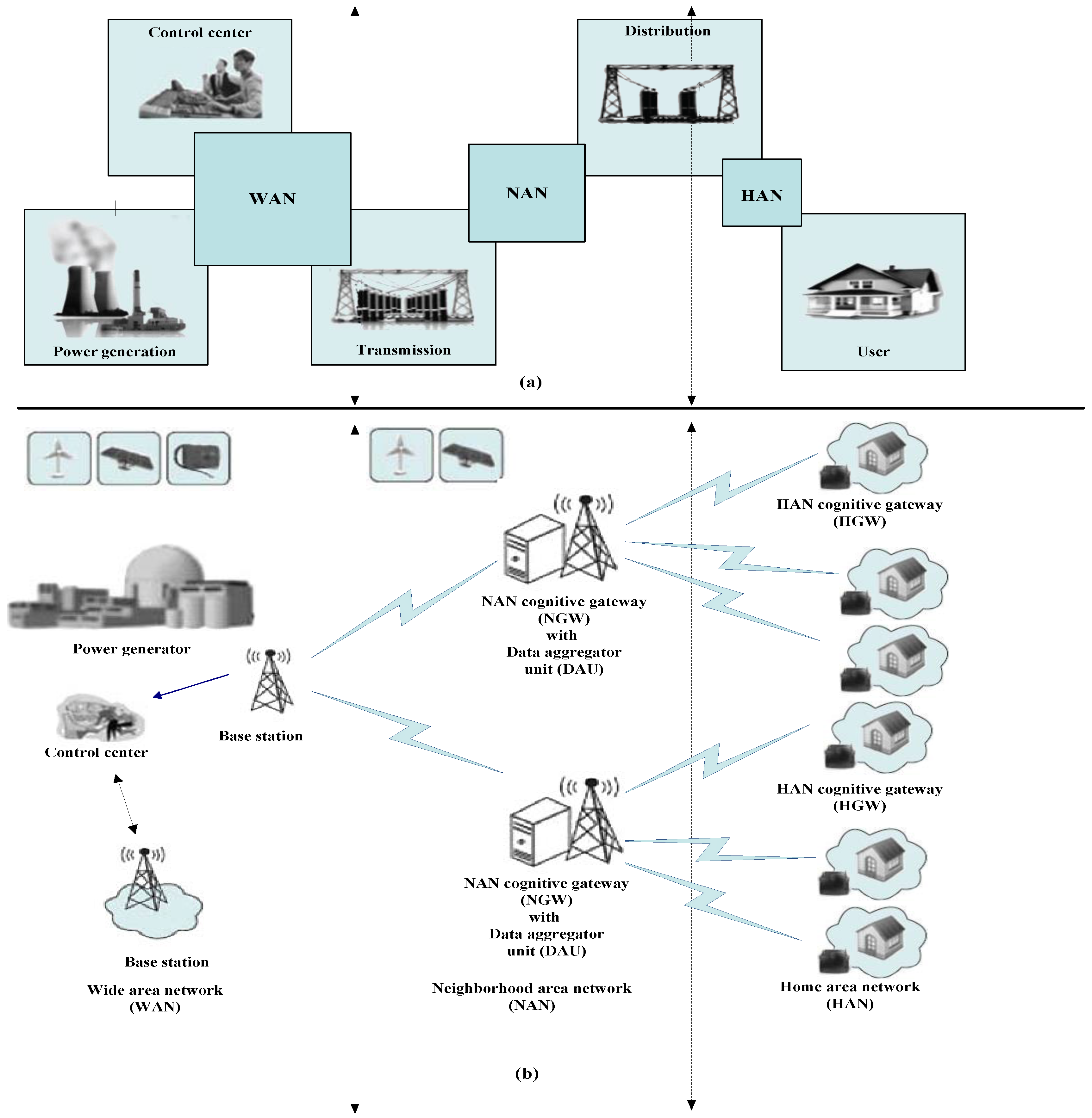
The communication infrastructure of the smart grid provides three fundamental functionalities, including, sensing, transmitting, and monitoring for control. The sensing functionality is carried out by different types of embedded sensors and smart meters to detect the status of different areas of the grid in a real-time manner. The smart grid should support the two-way data transmission links between the control centers and the sensors [56]. Control instructions are transmitted from/to sensors or smart meters fixed in different places to support reliable and stable access to grid components and also to guarantee the high-performance operations of the smart grid. To fulfill these issues, smart grid infrastructure consists of three parts different in their location and size [57]. These parts can be summarized in the following points:

(a)

Home Area Network (HAN): The HAN uses a local area wireless or short-range communication to support real-time data transmission of a smart meter, power load control, and dynamic pricing by connecting different kinds of devices with actuators, sensors, in-home display, and smart meter. Wireless technologies are the suitable choices for HANs because of their flexibility, high performance of control, and low installation cost. An example of this technology is ZigBee, which is a suitable for HANs due to high interoperability [58,59]. HAN gateway is used to transmit data to an external entity such as Data Aggregator Unit (DAU). DAU is used to collect the smart meters’ data and transfer these data to control center. The HAN gateway can be standalone within home devices (e.g., programmable thermostat or in-home display) or alternatively integrated with HAN smart meter.

(b)

Neighborhood Area Network (NAN): The NAN connects a set of HANs together and also connects HANs with the control center. As shown in Figure 3b the mission of the HAN gateway is to send meter data to a DAU through the NAN. The DAU communicates with the HAN gateway using network technologies such as 801.11 s, RF mesh, WiMAX, 3G, 4G, and LTE. DAU can operate as a NAN gateway to transfer the collected data to a Meter Data Management System (MDMS), which is a control center used to collect data, process the meter power consumption data, store these data, generate a report about power generation, and manage the place of power distribution [58,60].

(c)

Wide Area Network (WAN): The WAN connects remote systems together in a smart grid. Examples of these systems are MDMS, Advanced Metering Infrastructure (AMI), which is used to aggregate the data from the smart meter, and Synchronous Optical Network (SONET). The Wide-Area Measurement System (WAMS) in a WAN is responsible to manage the transmission and aggregate data for control purposes and power load measurement. The WAN supports a backhaul connection among distributed subsystems, power generators, customer premises, and the public utility. In this case, the backhaul can support different kinds of technologies (e.g., broadband wireless access or cellular network) to transmit the meter data from a NAN to the DAU, after that, from the DAU to MDMS at local offices. A WAN gateway supports broadband connection such as WiMAX, satellite, and 3G to collect the required data [58,61].

A smart grid uses a hierarchical communications infrastructure to increase the performance of the network. However, smart grids have as a main challenge the increasing number of smart meters [62]. This increases the network delay, especially in crowded cities. For this reason, in this paper, we are going to minimize the end-to-end delay of WSN to increase its QoS. The hierarchical communications infrastructure of the smart grid is shown in Figure 3 [63].

Table 5. Summary of the smart grid characteristics based on hierarchical communications infrastructure [62,63].

Cognitive Area Networks	Wide Area Network (WAN)	Neighborhood Area Network (NAN)	Home Area Network (HAN)
Network topology	Centralized	Centralized	Centralized/decentralized
Spectrum band	Licensed band	Licensed band	Unlicensed band
Favorable network protocol	WiMax, 3GPP, RF Mesh, and satellite	801.11 s, RF mesh WiMax, 3 G, 4 G and LTE	IEEE 802.15.4
Network users	Spectrum broker, NGWs	HGWs, NGW	Smart sensors/meters/actuators, HGW
Featured strategy	Optimal spectrum leasing	Hybrid dynamic spectrum access	Cross-layer spectrum sharing
Application	Demand Resource and load management	Advanced metering infrastructure, demand resource, and load management	Advanced metering infrastructure, demand resource, etc.
Key techniques	Join spectrum management	Spectrum handoff, guard channel	Power coordination, access control

summarizes the smart grid characteristics based on hierarchical communications infrastructure [63,64]. Based on these features, we can notice that HAN is the only part of the smart grid that used the short-range communication protocols such as IEEE 802.15.4/ZigBee. The features of IEEE 802.15.4 are summarized in the following subsections.

IEEE 802.15.4 Protocol

IEEE 802.15.4/ZigBee standard is a modern wireless communication protocol. This protocol has a set of features that make it convenient to use with smart grid, including cheap price, low power consumption, low complexity, and good data rate. This protocol supports Carrier Sense Multiple Access (CSMA), which is used to access the medium with no collision. IEEE 802.15.4/ZigBee standard can be operated on various license-free frequency bands. These bands support different numbers of channels, data transmission rate, and different frequency ranges [64]. The available radio frequency bands that are supported by IEEE 802.15.4/ZigBee standard [65] are summarized in

Table 6. A set of radio frequency bands along with their characteristics that supported by IEEE 802.15.4/ZigBee standard [67].

Frequency Bands	Area	Data Rate (Kbps)	Frequency Range (MHz)	Number(s) of Channel
915 MHz	Australia, America	40	902–928	10 channels
2.4 GHz	Asia, Worldwide	250	2405–2480	16 channels
868 MHz	Europe	20	868.3	1 channel

along with their characteristics. In this work, we choose the 2.4 GHz band because it can operate on 16 channels with a higher data transmission rate equal to 250 Kbps, and very important thing; this band is allowed to be applied in Asia [66,67].

Different types of network topologies can be supported by IEEE 802.15.4/ZigBee such as star topology, peer to peer (mesh topology), and cluster tree topology [68]. The data frame structure that is supported by IEEE 802.15.4/ZigBee is summarized in

Table 7. Data frame structure of The IEEE 802.15.4 [53].

		MAC Sublayer	2 Bytes	1 Byte	0–20 Bytes	Variable	2 Bytes
			Frame Control	Sequence Number	Address Fields	Data Payload	Frame Check Sequence
			MAC Header			MAC Service Data Unit	MAC Footer
PHY layer	Sync Header	PHY Header	PHY Service Data Unit (PSDU)
5 bytes			1 byte	≤127 bytes

. This structure consists of four parts including, MAC command frame, data frame, beacon frame, and acknowledgment frame. Based on Table 7, the MAC packet size that is supported by IEEE 802.15.4/ZigBee is equal to 127 bytes. In addition, 114 bytes are the maximum packet payload size that is supported by IEEE 802.15.4/ZigBee [53].

6. Methodology and Experimental Setup

In this section, we focus on the HAN part of the smart grid. This part consists of IEEE 802.15.4/ZigBee smart sensors that embedded in different types of home appliances. These sensors operate based on MicaZ platform [69]. The characteristics of MicaZ platform are summarized in

Table 8. Features of MicaZ platform [70].

Features	Value	Remarks
Frequency band	2.4 GHz band	License-free band (ISM band)
Data rate	250 kbps	-
EEPROM	4K bytes	-
Operating system	TinyOS	Open-source
Battery	2× AA batteries	Attached pack
Energy consumption in startup mode	8 mA	-
Energy consumption in communication mode	19.7 mA	-
User interface	3 LEDs	Red, green and yellow
Indoor range	20 m to 30 m	1/2 wave dipole antenna
Outdoor range	75 m to 100 m	1/2 wave dipole antenna

[70].

The MicaZ platform is a good choice for the smart grid because it operates with low power consumption, works on the license-free band (ISM band), and covers up to 30 m of home or building area. However, this platform has limited energy resource, which operates based on 2× AA batteries. The misuse of the devices will deplete the battery power and decrease the node lifetime. On the other hand, the network delay will be increased with an increasing number of smart meters in HANs, especially in crowded cities. Therefore, if the delay increases, the number of dropped packets will be increased and retransmitting the dropped packets will consume more power and time. Therefore, we used four algorithms namely, the MOSFP, OMOPSO, NSGA-II, and SPEA2 algorithms, to maximize both the network energy efficiency and network throughput; in particular we use these algorithms to minimize both the network end-to-end delay and end-to-end latency.

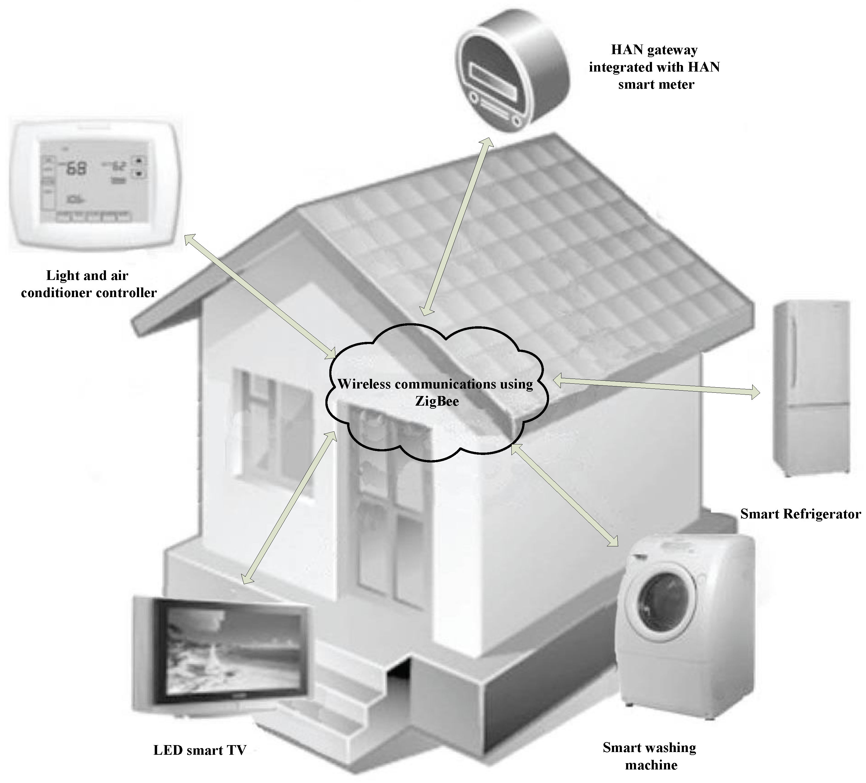
We assume that the smart home consists of four sensors embedded in four appliances such as a smart refrigerator, smart light and air conditioner controller, smart washing machine and smart TV. These sensors operate over the 2.4 GHz ISM band to communicate with a smart home gateway that is integrated with the smart meter using a star topology. The proposed network is depicted in Figure 4. These sensors consume 8 mA in start-up mode and 19.7 mA when the sensor is in communication mode [70]. 802.15.4/ZigBee can support a low sampling rate from 0 to 250 Hz [71]. This can satisfy the requirements of the smart grid. The BER in normal status has a value of 0.0004 [72]. By knowing these values and the other values such as the IEEE 802.15.4 physical and MAC headers, we can measure the objective functions (Equations from (8) to (19)). We focused on minimizing both the network end-to-end delay and end-to-end latency and also maximizing both network energy efficiency and packet throughput by changing the packet payload size. Packet payload size plays a significant role in determining the optimal value of these features, which if the packet payload size increases, the network delay will be increased and the energy efficiency will be decreased.

We compile the JMetal 4.5 tool in NetBeans IDE 8.0.2 by using the Java version. The test environment is a 3 GB RAM, Intel dual-core CPU-T3200, running Windows 7.

Table 9. Parameters of the algorithms.

Parameters	MOSFP	OMOPSO	NSGA-II	SPEA2
Population size	20	20	20	20
Archive size	(winner) 20	20	(Elite) 20	20
Mating pool size	-	-	-	20
Maximum generation	250	250	250	250
Crossover probability	-	-	0.9	0.9
Mutation probability	1/d where d is the variable code size

summarizes the parameters of all the optimization algorithms that are used in this study. Most of these parameters and settings are assigned as recommended in [15,53]. On the other hand,

Table 10. Simulation parameters.

No.	Parameter	Values
0	Time of interframe space (Tifs)	192 μs
1	Transceiver’s transmitting to receiving turnaround time (TTA)	192 μs
2	The duration of one backoff slot (Tboslot)	320 μs
3	Use of ACKs	N0
4	PHY header (LPHY)	6 bytes
5	MAC header (LMHR)	11 bytes
6	MAC footer (LMFR)	2 bytes
7	The default minimum value of backoff exponent (macMinBE)	3
8	The default maximum value of backoff exponent (aMaxBE)	5
9	Number of sensors (n)	5
10	Transceiver’s raw data rate (Rdata)	250 kbps
11	The energy consumption in startup mode (Es)	8 mA
12	Energy consumption through the communication (Ec)	19.7 mA
13	Sampling rate	250 Hz
14	Bit Error Rate (BER)	0.0004

summarizes the parameters needed to evaluate the network modelling part. The procedure of maximizing both network energy efficiency and packet throughput, and minimizing both the network end-to-end delay and end-to-end latency are summarized for each algorithm in Figure 5, Figure 6, Figure 7 and Figure 8.

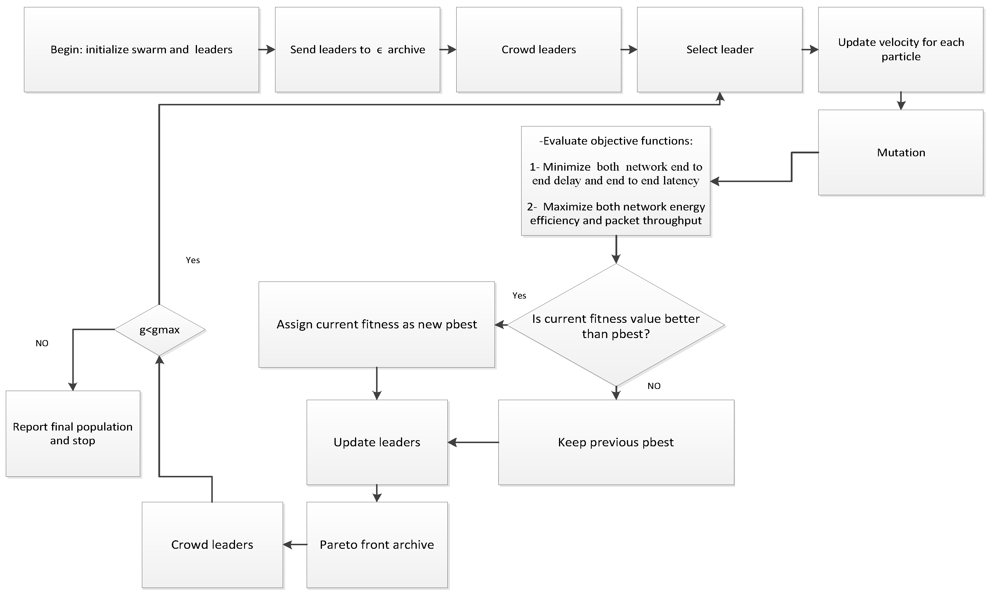
The procedure of OMOPSO, summarized in Figure 5, begins by initializing the parameter of packet payload size that varies from 0 to 114 bytes based on the IEEE 802.15.4 data frame. After that, the algorithm performs the archive on the leaders and crowding operator on the elected leaders. The algorithm checks the state of the size of the leaders in which, if their size greater than the required size, the algorithm keeps the best leaders and eliminates the others. Hence, the velocity update rule comes to take place on the procedure, where is applied to each member of the population, after that, it performs the mutation operation. Moreover, the algorithm evaluates the objective functions (Equations from (8) to (19)), which uses the population members to minimize both the network end-to-end delay and end-to-end latency and also to maximize both energy efficiency and network throughput. In addition, the algorithm compares the new fitness of each individual with its old fitness value. The algorithm stores the new fitness just in case of the new one is better than the old. Then, the algorithm updates the leaders of the new generation of the population follows by archiving and crowding operators on the leaders. Finally, the algorithm checks the number of iterations. If the maximum generations (the value of 250 generations as in Table 9) is reached the algorithm will terminate, otherwise, the algorithm will repeat the past steps.

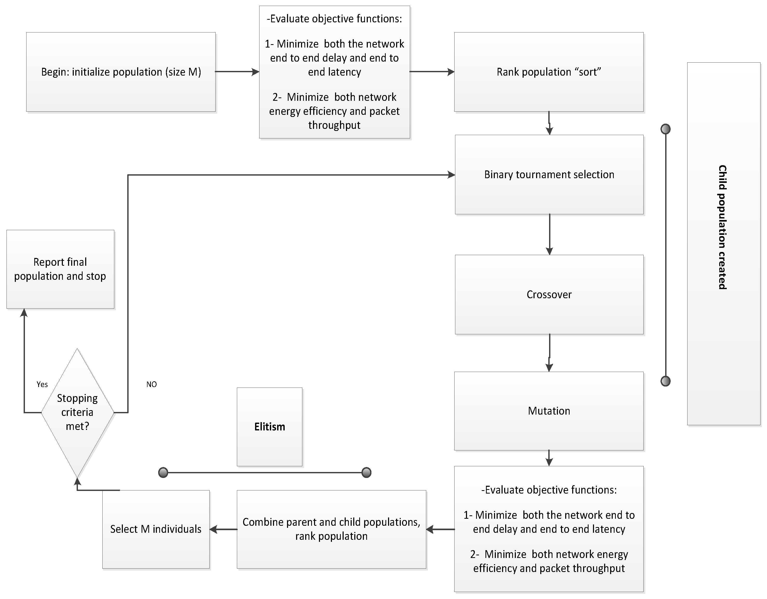
The procedure of NSGA-II, depicted in Figure 6, begins by initializing the packet payload size parameter. The lower limit and upper limit of this parameter are 0 byte and 114 bytes based on the IEEE 802.15.4 data frame, respectively. Based on the first population of this parameter, the algorithm evaluates the objective functions (Equations from (8) to (19)), which minimizes both the network end-to-end delay and end-to-end latency, and also maximizes both power efficiency, and network throughput. Moreover, the algorithm ranks the population based on non-dominated solutions and performs selection, crossover, and mutation operations to generate new population (child population). Based on the results of the previous steps, the algorithm uses the child population to evaluate the same objective functions. After that, the algorithm combines the child population with the old population. Later, it ranks the produced populations from the best to worst results. At the end, the algorithm checks on the number of iterations, in case it more than the maximum number of iterations (the value of 250 generations as in Table 9), the algorithm will terminate.

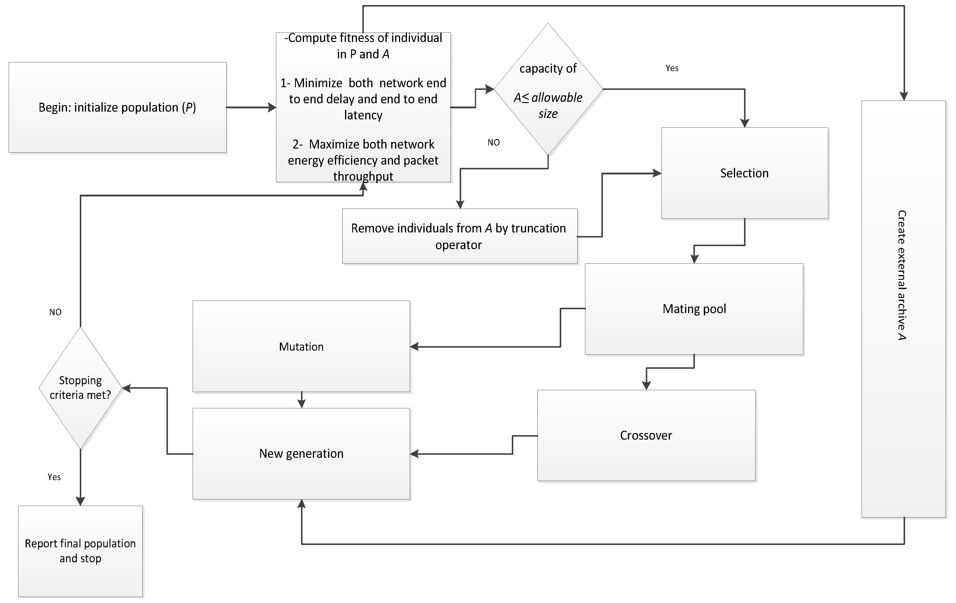
Based on Figure 7, we can summarize the procedure of SPEA2 as follows: the algorithm begins the procedure by initializing the packet payload value, which is varied in the range of 0 to 114 bytes based on the IEEE 802.15.4 data frame. After that, SPEA2 uses the first population to evaluate the objective functions to minimize the network end-to-end delay and end-to-end latency and also maximize the network throughput and energy efficiency. Hence, the algorithm uses the values of the fitness function to perform the selection operator. After selection, the algorithm generates the mating pool. This pool is a set of population that both mutation and crossover operations are applied on them in order to generate a new population.

At the end, the algorithm checks the number of iterations, which in case it reaches the maximum generations (the value of 250 generations as in Table 9), the algorithm will terminate, and else, the algorithm will repeat the previous steps.

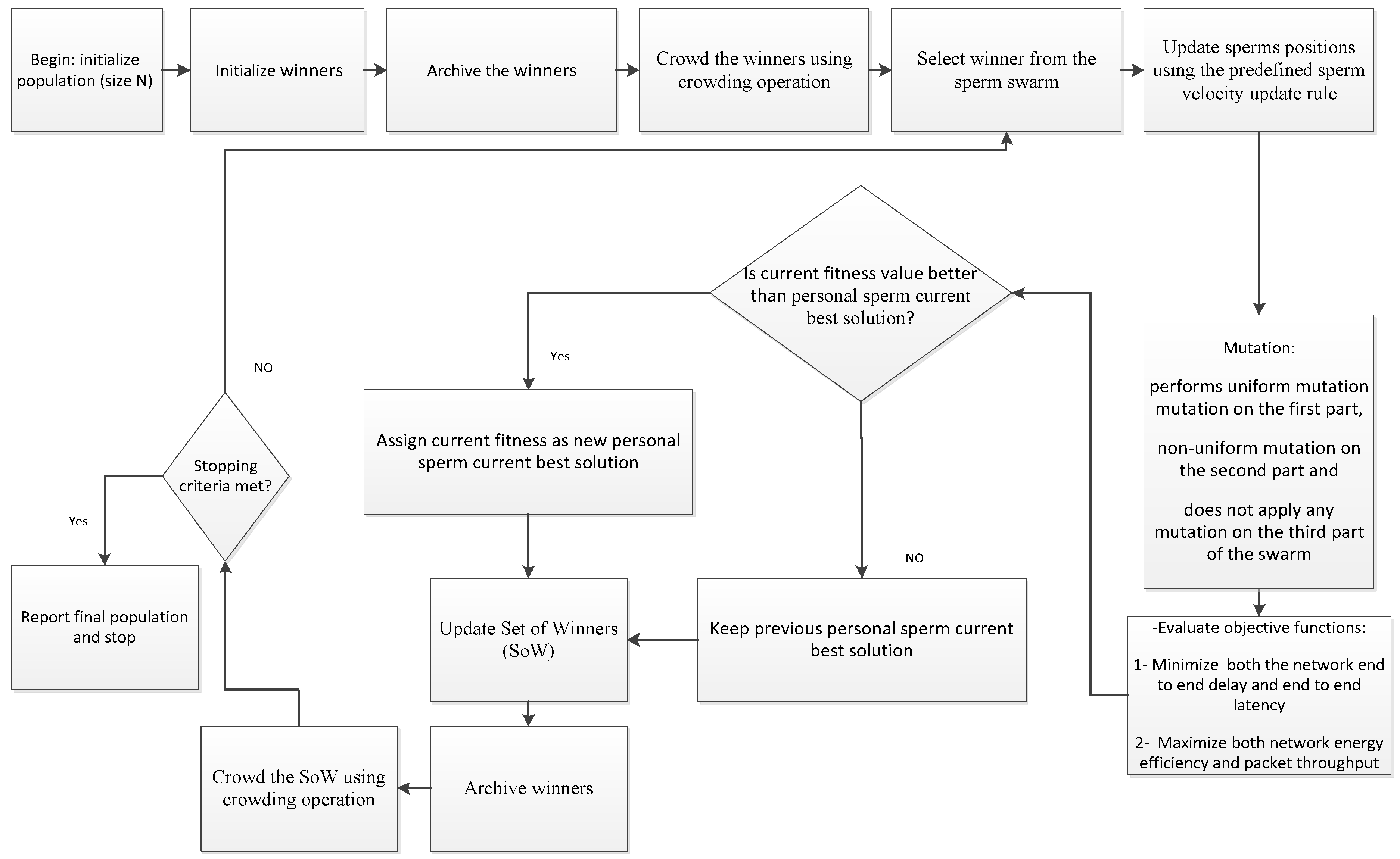
Like OMOPSO, NSGA-II and SPEA2, MOSFP begins the procedure by initializing the packet payload size parameter, which is varied in the range of 0 to 114 bytes based on the IEEE 802.15.4 data frame (see Figure 8). After that, the algorithm archives the required number of winners. Then, it groups the winners based on the crowding operation. In the case of the size of the winners is greater than the defined maximum size of winners, the algorithm keeps the best winners and eliminates the other winners. Hence, it applies the velocity update rule on each individual of the population. In addition, it performs mutation to prepare the population for evaluation. In the evaluation part, MOSFP uses the population to minimize both the end-to-end delay and end-to-end latency of the network and to maximize both the energy efficiency and packet throughput. The algorithm changes the fitness value of each individual just in the case of the new fitness value of the individual is better than the old one. Later on, the algorithm updates the set of winners, after that, it performs archiving and crowding operators on the winners. At the end, if the number of maximum generations is not reached (the value of 250 generations as in Table 9), the algorithm will repeat the prior steps, else, the algorithm will terminate.

7. Experimentation and Results

In this study, the experimental results are analyzed in two ways. First, the outcomes from each algorithm for four objective functions based on ten runs are analyzed using one-way ANOVA (Tukey’s test). In this test, the mean difference between the algorithms is significant if the p-value is smaller than 0.05.

Second, the Pareto front set that obtained by the four algorithms is analyzed for the four objective functions. The Pareto front is very important to illustrate the trade-offs between a set of optimization functions (objective functions). From the Pareto observation, we can know the optimal value of packet payload size that achieves the optimal values for a set of conflict objective functions.

7.1. Comparisons between the Four Algorithms Using Statistical Analysis

Table 11. Comparison between SPEA2, MOSFP, OMOPSO, and NSGA-II for four objective functions. The highlighted background with bold font represents the best average for the respective objective function.

Objective Functions	Algorithms	Mean	Std. Dev.	Std. Error	95% Confidence Interval for Mean		Min	Max
					Lower Bound	Upper Bound
Energy Efficiency	SPEA2	0.285	0.181	0.013	0.260	0.310	0.096	0.602
	MOSFP	0.401	0.185	0.013	0.375	0.427	0.096	0.602
	OMOPSO	0.392	0.188	0.013	0.366	0.418	0.096	0.602
	NSGA-II	0.387	0.186	0.013	0.361	0.413	0.096	0.602
Packet Throughput	SPEA2	0.398	0.828	0.059	0.282	0.513	0.010	3.161
	MOSFP	0.791	1.074	0.076	0.642	0.941	0.010	3.154
	OMOPSO	0.776	1.079	0.076	0.626	0.926	0.010	3.154
	NSGA-II	0.725	1.054	0.075	0.578	0.872	0.010	3.158
End-to-End Delay	SPEA2	1.105	0.422	0.030	1.047	1.164	0.240	1.493
	MOSFP	0.840	0.454	0.032	0.777	0.903	0.240	1.492
	OMOPSO	0.858	0.459	0.032	0.794	0.922	0.240	1.492
	NSGA-II	0.874	0.453	0.032	0.811	0.937	0.240	1.493
End-to-End Latency	SPEA2	6.597	4.927	0.348	5.910	7.284	0.279	15.579
	MOSFP	3.880	4.539	0.321	3.247	4.513	0.279	15.533
	OMOPSO	4.137	4.741	0.335	3.476	4.798	0.279	15.535
	NSGA-II	4.185	4.673	0.330	3.534	4.837	0.279	15.601

summarizes the objective functions, namely, energy efficiency, packet throughput, end-to-end delay and end-to-end latency, from ten runs for each algorithm. The statistical analysis using one-way ANOVA (Tukey’s test) outlined in

Table 12. Analysis of one-way ANOVA (Tukey’s test) between SPEA2, MOSFP, OMOPSO and NSGA-II for four objective functions.

Objective Functions	Algorithm (I)	Algorithm (J)	Mean Difference (I-J)	Std. Error	p-Value	95% Confidence Interval
						Lower Bound	Upper Bound
Energy Efficiency	MOSFP	SPEA2	0.116	0.018	<0.001 *	0.068	0.163
		OMOPSO	0.009	0.018	0.965	−0.039	0.056
		NSGA-II	0.013	0.018	0.888	−0.034	0.061
Packet Throughput	MOSFP	SPEA2	0.394	0.101	<0.001 *	0.133	0.655
		OMOPSO	0.015	0.101	0.999	−0.246	0.276
		NSGA-II	0.066	0.101	0.916	−0.195	0.327
End-to-End Delay	MOSFP	SPEA2	−0.265	0.045	<0.001 *	−0.380	−0.150
		OMOPSO	−0.018	0.045	0.977	−0.133	0.097
		NSGA-II	−0.034	0.045	0.872	−0.149	0.081
End-to-End Latency	MOSFP	SPEA2	−2.718	0.472	<0.001 *	−3.933	−1.502
		OMOPSO	−0.257	0.472	0.948	−1.473	0.958
		NSGA-II	−0.306	0.472	0.917	−1.521	0.910

* The mean difference is significant at the 0.05 level.

shows that MOSFP significantly outperforms SPEA2 in which, MOSFP substantially increase the energy efficiency (0.116, p ≤ 0.001) and packet throughput (0.394, p ≤ 0.001), and decrease the end-to-end delay (−0.265, p ≤ 0.001) and end-to-end latency (−2.718, p ≤ 0.001) compared to SPEA2. These mean differences also represent that MOSFP outperforms SPEA2 by 41%, 99%, 24% and 41% in term of energy efficiency, packet throughput, end-to-end delay and end-to-end latency respectively. However, no significant mean difference is observed between MOSFP and the rest of the algorithms i.e., OMOPSO and NSGA-II for all objective functions. This indicates that MOSFP outperforms OMOPSO and NSGA-II with a small mean difference between them in the range of 2% to 9%.

Another aspect that will be highlighted in this sub-section is the consistency of the algorithm to perform between runs. A more stable algorithm will result in a smaller standard deviation of the objective function. From the experiments, SPEA2 has results in a more consistent performance for three objective functions between runs among the algorithms. The standard deviations of SPEA2 are approximately 3%, 23% and 7% much smaller compared to others for energy efficiency, packet throughput, and end-to-end delay respectively. In end-to-end latency, MOSFP has shown a more consistent performance where its standard deviations are 8%, 4% and 3% smaller than SPEA2, OMOPSO and NSGA-II, respectively.

Overall, the MOSFP algorithm obtained the best average of all objective functions while the OMOPSO algorithm is in the second, followed by NSGA-II and SPEA2. In terms of performance consistency, the SPEA2 results are shown to be more consistent in energy efficiency, packet throughput, and end-to-end delay whereas MOSFP is shown to be more consistent in end-to-end latency.

7.2. Analysis of Pareto-Optimal Set of the Four Algorithms

As we introduced previously, the multi-objective optimization problems are a set of conflict optimization objective functions that consist of minimization and maximization functions. Pareto optimality concept is emerged to manage the trade-offs between these objectives. This concept is proposed by Vilfredo Pareto in 1906 [73]. Pareto optimality operates mainly based on the Pareto front set, which is used to balance the conflict objective functions. Based on the Pareto front of each objective function, two concepts should be defined as follows:

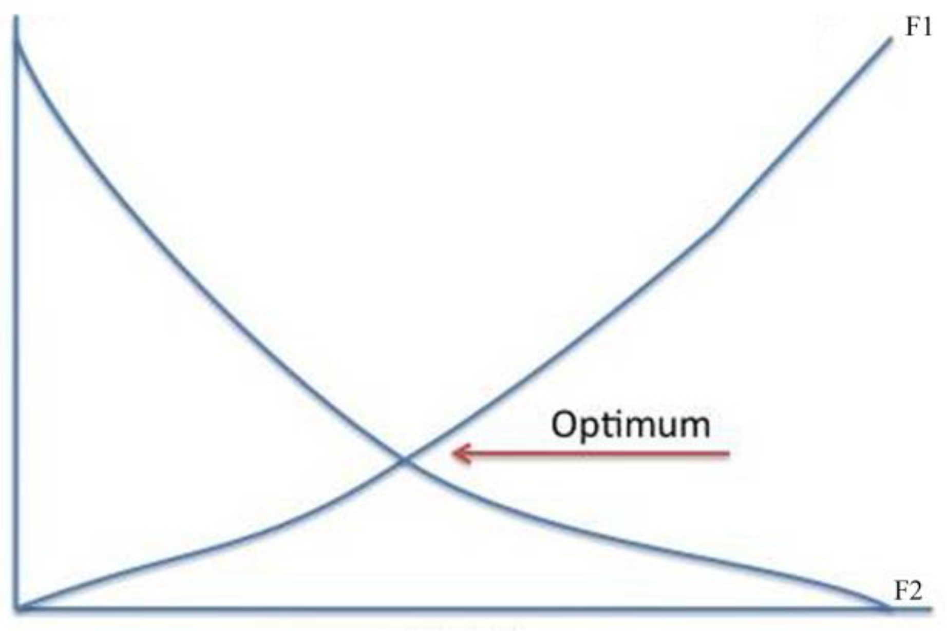
(a)

The Marginal concept of optimality: the optimal value based on this concept can be illustrated by the intersection points between a set of objective functions, which some of them minimization and the others are maximization [74]. Figure 9 presents the optimum value based on the intersection between two objective functions [75].

(b)

The knee point: is a point on the Pareto front curve, which is referred to the most preferred solution. Knee point can be estimated by determining the greatest reflex angle that bends of the front from its left to its right or vice-versa. Based on Figure 10 [76], three points called A, B, and C are used to illustrate the knee point concept. The B point is considered as the knee point, which makes the greatest reflex angle between C point on the right side of the front and the A point on the left side of the front.

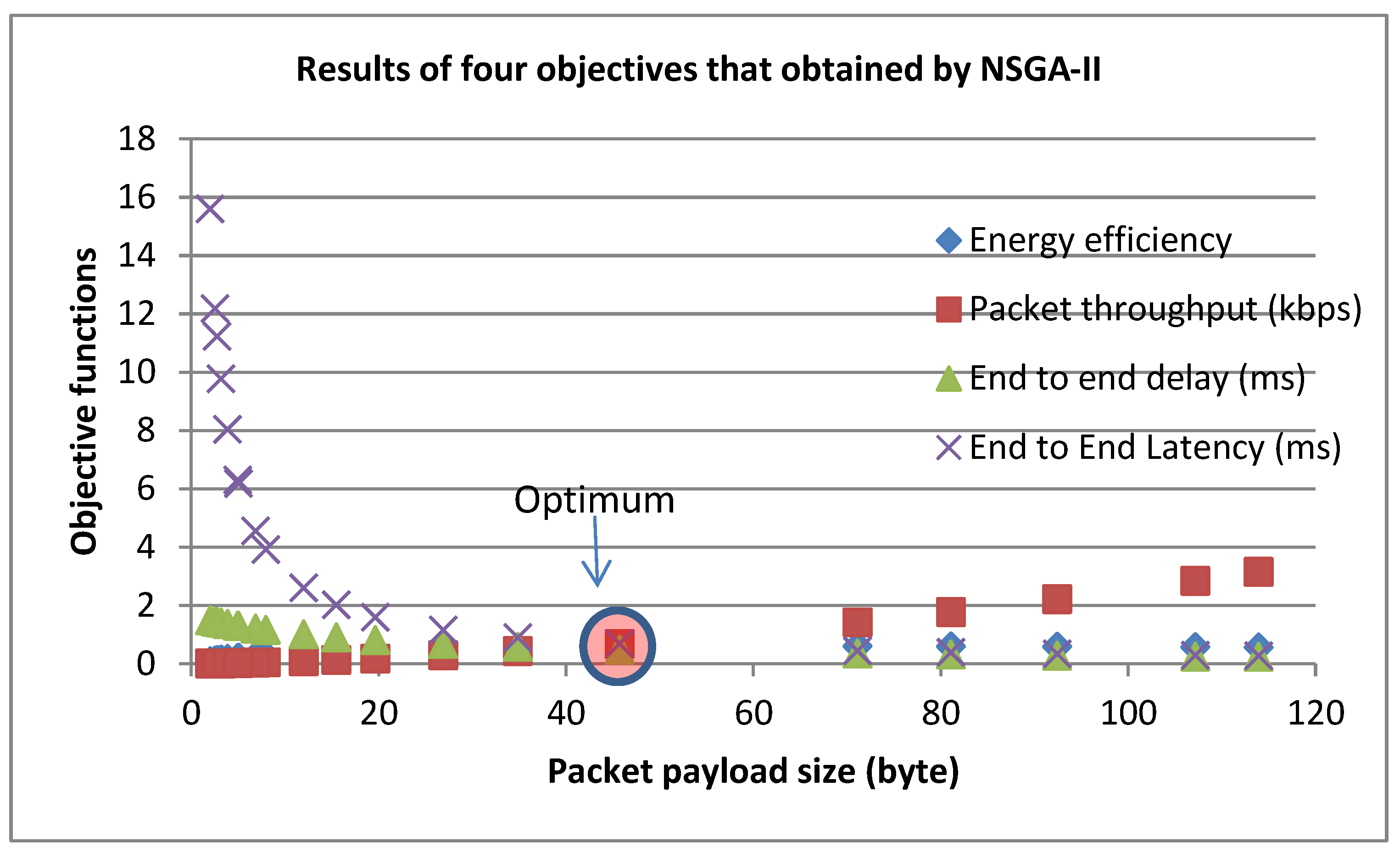
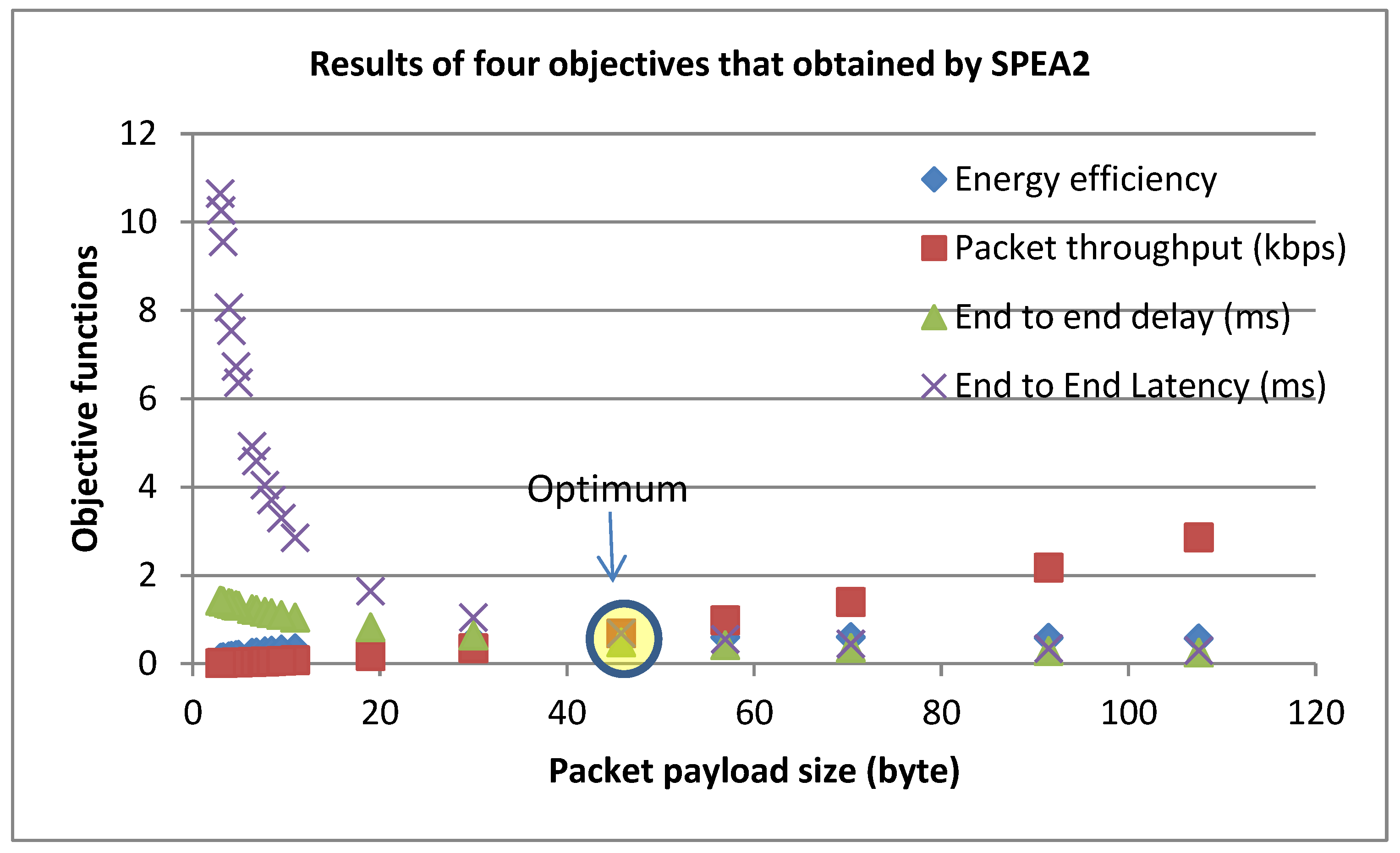
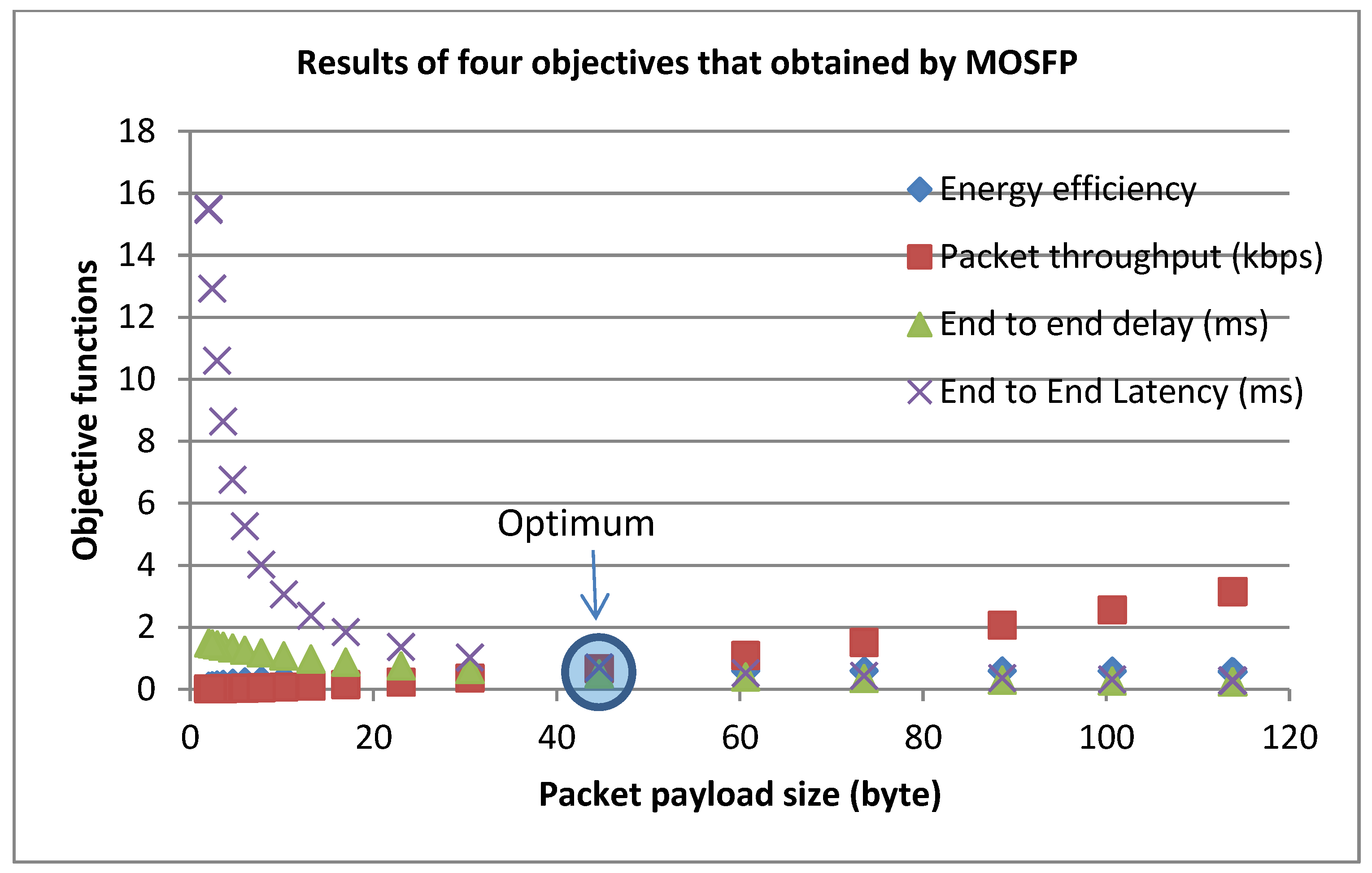
Figure 11, Figure 12, Figure 13 and Figure 14 show a sample of optimizing the four objective functions denoted by maximizing both energy efficiency and packet throughput and also minimizing both end-to-end delay and end-to-end latency using four algorithms. These algorithms are MOSFP, OMOPSO, NSGA-II, and SPEA2. From the results, the value of end-to-end latency decreases sharply and end-to-end delay decreases slightly until the value of packet payload size reaches 45 bytes, after that, both of them stabilize below 2 when the packet payload size is beyond 45 bytes. On the other hand, the packet throughput increases slightly until the value of packet payload size reaches 45 bytes, after that, it increases dramatically until the value of packet payload size reaches 114 bytes. Furthermore, the energy efficiency increases slightly until the value of packet payload size reaches 45 bytes, after that, it stabilizes above the 0.5 when the packet payload size increases more than 45 bytes. From the figures, we can notice that the optimum points are represented by different colors (i.e., green, red, yellow and blue), which are the intersection points of all the objective functions. These points are created when the packet payload size equal to 45 bytes.

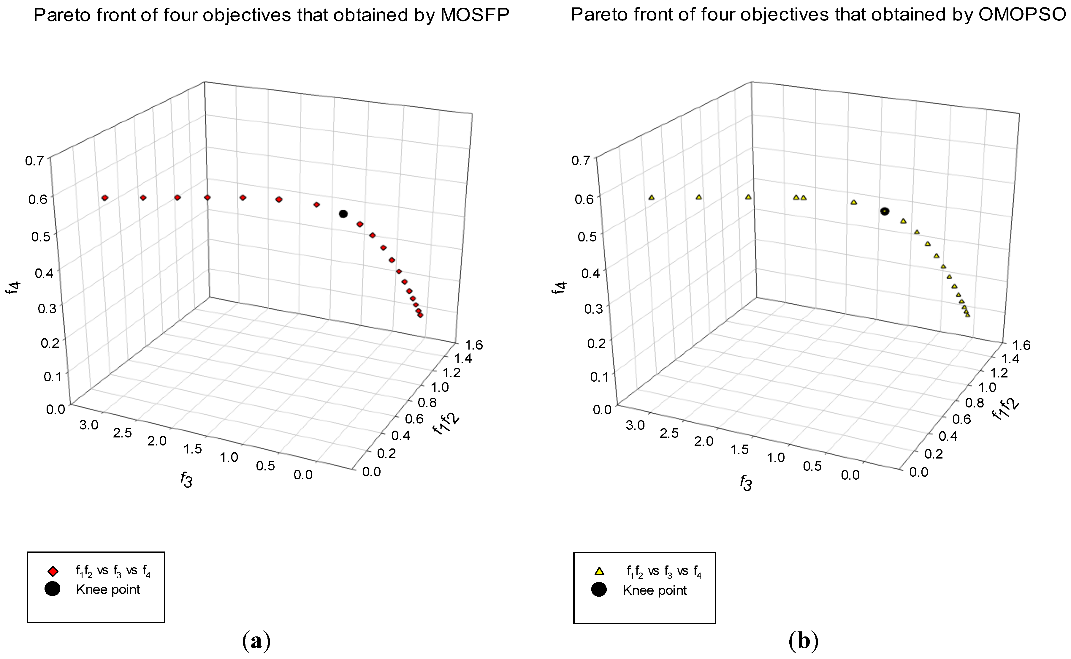
Figure 15 presents the Pareto optimal front obtained from all the algorithms at the end of 250 generations where f₁ represents the end-to-end delay, f₂ represents the end-to-end latency, f₃ represents the network throughput, and f₄ represents the energy efficiency. Both MOSFP and OMOPSO produce 19 non-dominated solutions related to the Pareto front, while both NSGA-II and SPEA2 produce 18 non-dominated solutions for the same objective functions. This proves the ability of MOSFP which obtained 19 values of getting good results, compared to SPEA2 and NSGA-II. In addition, MOSFP has the best spread and distribution of solutions related to the true Pareto front while the OMOPSO is in the second followed by NSGA-II and SPEA2 as outlined in Figure 15.

Based on Figure 7, we can summarize the procedure of SPEA2 as follows: the algorithm begins the procedure by initializing the packet payload value, which is varied in the range of 0 to 114 bytes based on the IEEE 802.15.4 data frame. After that, SPEA2 uses the first population to evaluate the objective functions to minimize the network end-to-end delay and end-to-end latency and also maximize the network throughput and energy efficiency. Hence, the algorithm uses the values of the fitness function to perform the selection operator. After selection, the algorithm generates the mating pool. This pool is a set of population that both mutation and crossover operations are applied on them in order to generate a new population.

8. Conclusions

In this paper, we study the problems of smart grid applications, especially in HANs, which utilize a wide variety of sensor-based devices that operate using short-range communication technologies such as IEEE 802.15.4. In addition, these sensors operate using batteries. The misuse of these devices will decrease the lifetime of the network and lead to a rapid node death. For this reason, this paper uses a theoretical analysis to mitigate these problems using our proposed algorithm (MOSFP) along with three well-known algorithms in the multi-objective optimization field, namely OMOPSO, NSGA-II, and SPEA2. These algorithms have been used to optimize four network features that are used to evaluate the QoS of the network. These features consist of network end-to-end delay, end-to-end latency, network throughput, and energy efficiency. The parameter of a physical layer such as packet payload size is considered to maximize both network throughput and energy efficiency, and also to minimize both the network end-to-end delay and end-to-end latency. The results have been reported using two different ways. In a first way, the statistical analysis of one-way ANOVA (Tukey’s test) between the algorithms is conducted for each objective function based on ten-time runs. In a second way, a sample of the Pareto-optimal set of each algorithm has been analyzed using the knee point and intersection point concepts.

The mean difference from one-way ANOVA (Tukey’s test) indicates that our algorithm (MOSFP) significantly outperformed SPEA2 in optimizing the proposed features while no significant mean difference is observed between MOSFP and, OMOPSO and NSGA-II. However, the overall performance of MOSFP outperformed OMOPSO, NSGA-II and SPEA2 by 3%, 6% and 51%, respectively. Furthermore, MOSFP found the best average value of energy efficiency feature compared with the other algorithms, which is very important to increase the lifetime of the network. In the second test, the Pareto front results illustrated that MOSFP algorithm, which has a good spread and approximation of the true Pareto front of the proposed network features, outperformed the other algorithms. This is very clear with the Pareto front of MOSFP in Figure 15, which obtained on 19 non-dominated solutions related to Pareto front rather than NSGA-II, and SPEA2. Furthermore, we can notice that MOSFP has the best spread and distribution of solutions related to the true Pareto front while the OMOPSO is in the second, followed by NSGA-II and SPEA2, as summarized in Figure 15. Overall, the knee point and the intersection point of all the Pareto-optimal sets for all the algorithms illustrated that the optimal value of packet payload size is equal to 45 bytes, a value which manages a trade-off between the maximization and minimization objective functions. This paper takes the smart grid as the case study as this network is affected by end-to-end delay, especially in dense cities.

The objective functions in this paper may have their limitations. Other variables may exist in real implementation that may affect the outcome of the studies. Therefore, the value of the payload size resulting from the experiment should be tested in real environmenta in the future to ensure the reliability of the proposed method. Finally, one aspect that we would like to explore in the future is the hybridization between our algorithm (MOSFP) and other algorithms such as genetic algorithms to increase the algorithm convergence and we will use it to optimize some problems related to data aggregation [77,78] in WSNs.

References

1. Akyildiz, I.F.; Melodia, T.; Chowdury, K.R. Wireless multimedia sensor networks: A survey. IEEE Wirel. Commun. 2007, 14, 32–39. [Google Scholar] [CrossRef]
2. Abu-Sharkh, O.M.; AlQaralleh, E.; Hasan, O.M. Adaptive device-to-device communication using Wi-Fi Direct in smart cities. Wirel. Netw. 2016, 22, 1–17. [Google Scholar] [CrossRef]
3. Aguirre, E.; Lopez-Iturri, P.; Azpilicueta, L.; Astrain, J.J.; Villadangos, J.; Santesteban, D.; Falcone, F. Implementation and analysis of a wireless sensor network-based pet location monitoring system for domestic scenarios. Sensors 2016, 16, 1384. [Google Scholar] [CrossRef] [PubMed]
4. Doudou, M.; Djenouri, D.; Barcelo-Ordinas, J.M.; Badache, N. Delay-efficient MAC protocol with traffic differentiation and run-time parameter adaptation for energy-constrained wireless sensor networks. Wirel. Netw. 2016, 22, 467–490. [Google Scholar] [CrossRef] [Green Version]
5. Singh, R.; Singh, J. Security challenges in wireless sensor networks. Int. J. Comput. Sci. Inf. Technol. Secur. IJCSITS 2016, 6, 1–6. [Google Scholar]
6. Jia, J.; Chen, J.; Chang, G.; Tan, Z. Energy efficient coverage control in wireless sensor networks based on multi-objective genetic algorithm. Comput. Math. Appl. 2009, 57, 1756–1766. [Google Scholar] [CrossRef]
7. Yang, J.; Zhang, H.; Ling, Y.; Pan, C.; Sun, W. Task allocation for wireless sensor network using modified binary particle swarm optimization. IEEE Sens. J. 2014, 14, 882–892. [Google Scholar] [CrossRef]
8. Kukunuru, N.; Thella, B.R.; Davuluri, R.L. Sensor deployment using particle swarm optimization. Int. J. Eng. Sci. Technol. 2010, 2, 5395–5401. [Google Scholar]
9. Sagar, A.K.; Lobiyal, D. Coverage and lifetime maximization of wireless sensor network with multi-objective evolutionary algorithm. Int. J. Sci. Eng. Res. 2014, 5, 1194–1203. [Google Scholar]
10. Chaudhuri, K.; Dasgupta, D. Multi-objective evolutionary algorithms to solve coverage and lifetime optimization problem in wireless sensor networks. In Proceedings of the International Conference on Swarm, Evolutionary, and Memetic Computing (SEMCCO), Chennai, India, 16–18 December 2010; pp. 514–522. [Google Scholar] [CrossRef]
11. Sengupta, S.; Das, S.; Nasir, M.; Vasilakos, A.V.; Pedrycz, W. An evolutionary multiobjective sleep-scheduling scheme for differentiated coverage in wireless sensor networks. IEEE Trans. Syst. Man Cybern. Part C Appl. Rev. 2012, 42, 1093–1102. [Google Scholar] [CrossRef]
12. Naeem, M.; Pareek, U.; Lee, D.C. Swarm intelligence for sensor selection problems. IEEE Sens. J. 2012, 12, 2577–2585. [Google Scholar] [CrossRef]
13. Liu, K. Wireless sensor network target coverage algorithm based on energy saving. Acta Tech. 2016, 61, 49–62. [Google Scholar]
14. Bara’a, A.A.; Khalil, E.A.; Cosar, A. Multi-objective evolutionary routing protocol for efficient coverage in mobile sensor networks. Soft Comput. 2015, 19, 2983–2995. [Google Scholar] [CrossRef]
15. Hamdan, M.; Yassein, M.B.; Shehadeh, H.A. Multi-objective Optimization Modeling for the Impacts of 2.4-GHz ISM band Interference on IEEE 802.15.4 Health Sensors. In Information Innovation Technology in Smart Cities, 1st ed.; Ismail, L., Zhang, L., Eds.; Springer: Singapore, 2017; Volume 1, pp. 317–330. ISBN 978-981-10-1740-7. [Google Scholar]
16. Sierra, M.R.; Coello, C.C. Improving PSO-based multi-objective optimization using crowding, mutation and e-dominance, Evolutionary multi-criterion optimization. In Proceedings of the International Conference on Evolutionary Multi-Criterion Optimization, Guanajuato, Mexico, 9–11 March 2005; pp. 505–519. [Google Scholar] [CrossRef]
17. Deb, K.; Pratap, A.; Agarwal, S.; Meyarivan, T. A fast and elitist multiobjective genetic algorithm: Nsga-ii. IEEE Trans. Evolut. Comput. 2002, 6, 182–197. [Google Scholar] [CrossRef]
18. Eckart, Z.; Marco, L.; Lothar, T. SPEA2: Improving the strength pareto evolutionary algorithm for multiobjective optimization. In Proceedings of the Eurogen, Evolutionary Method for Design: Optimization and Control for Industrial Problem (EUROGEN’2001), Barcelona, Spain, 19–21 September 2001; pp. 1–21. [Google Scholar] [CrossRef]
19. Shehadeh, H.A.; ldris, M.Y.I.; Ahmedy, I. Multi-Objective Optimization Algorithm Based on Sperm Fertilization Procedure (MOSFP). Symmetry 2017, 9, 241. [Google Scholar] [CrossRef]
20. Ahmedy, I.; Shehadeh, H.A.; Idris, M.Y.I. An estimation of QoS for classified based approach and nonclassified based approach of wireless agriculture monitoring network using a network model. Wirel. Commun. Mob. Comput. 2017, 2017, 1–14. [Google Scholar] [CrossRef]
21. Yassein, M.B.; Hamdan, M.; Shehadeh, H.A.; Mrayan, L. A Novel approach for health monitoring system using wireless sensor network. Int. J. Commun. Antenna Propag. IRECAP 2017, 7, 271–285. [Google Scholar] [CrossRef]
22. Jawad, H.M.; Nordin, R.; Gharghan, S.K.; Jawad, A.M.; Ismail, M. Energy-Efficient Wireless Sensor Networks for Precision Agriculture: A Review. Sensors 2017, 17, 1781. [Google Scholar] [CrossRef] [PubMed]
23. Pinto, M.; Gámez, N.; Fuentes, L.; Amor, M.; Horcas, J.M.; Ayala, I. Dynamic reconfiguration of security policies in wireless sensor networks. Sensors 2015, 15, 5251–5280. [Google Scholar] [CrossRef] [PubMed]
24. Yan, X.; Du, H.; Ye, Q.; Song, G. Minimum-delay data aggregation schedule in duty-cycled sensor networks. In Proceedings of the International Conference on Wireless Algorithms, Systems, and Applications, Bozeman, MT, USA, 8–10 August 2016; Springer International Publishing: New York, NY, USA, 2016; pp. 305–317. [Google Scholar] [CrossRef]
25. Rout, D.K.; Das, S. Multiple narrowband interference mitigation using hybrid Hermite pulses for body surface to external communications in UWB body area networks. Wirel. Netw. 2017, 23, 387–402. [Google Scholar] [CrossRef]
26. Chen, D.; Liu, Z.; Wang, L.; Dou, M.; Chen, J.; Li, H. Natural disaster monitoring with wireless sensor networks: A case study of data-intensive applications upon low-cost scalable systems. Mob. Netw. Appl. 2013, 18, 651–663. [Google Scholar] [CrossRef]
27. Devidas, A.R.; Ramesh, M.V.; Rangan, V.P. High performance communication architecture for smart distribution power grid in developing nations. Wirel. Netw. 2016, 22, 1–18. [Google Scholar] [CrossRef]
28. Li, X.; Li, D.; Wan, J.; Vasilakos, A.V.; Lai, C.-F.; Wang, S. A review of industrial wireless networks in the context of industry 4.0. Wirel. Netw. 2017, 23, 23–41. [Google Scholar] [CrossRef]
29. Iturri, P.L.; Nazábal, J.A.; Azpilicueta, L.; Rodriguez, P.; Beruete, M.; Fernández-Valdivielso, C.; Falcone, F. Impact of high power interference sources in planning and deployment of wireless sensor networks and devices in the 2.4 GHz frequency band in heterogeneous environments. Sensors 2012, 12, 15689–15708. [Google Scholar] [CrossRef] [PubMed]
30. Guo, W.; Healy, W.M.; Zhou, M. Impacts of 2.4-GHz ISM band interference on IEEE 802.15. 4 wireless sensor network reliability in buildings. IEEE Trans. Instrum. Meas. 2012, 61, 2533–2544. [Google Scholar] [CrossRef]
31. Rajput, M.; Ghawte, U. Security Challenges in Wireless Sensor Networks. Int. J. Comput. Appl. 2017, 168, 24–29. [Google Scholar] [CrossRef]
32. Andréasson, N.; Evgrafov, A.; Patriksson, M. An Introduction to Optimization: Foundations and Fundamental Algorithms; Chalmers University of Technology Press: Gothenburg, Sweden, 2005; Volume 1, pp. 1–205. [Google Scholar]
33. Dreżewski, R.; Doroz, K. An Agent-Based Co-Evolutionary Multi-Objective Algorithm for Portfolio Optimization. Symmetry 2017, 9, 168. [Google Scholar] [CrossRef]
34. Meetei, K.T. A Survey: Swarm Intelligence vs. Genetic Algorithm. Int. J. Sci. Res. 2014, 3, 231–235. [Google Scholar]
35. Kennedy, J.; Eberhart, R. Particle swarm optimization. In Proceedings of the IEEE International Conference on Neural Networks, Perth, Australia, 27 November–1 December 1995; pp. 1942–1948. [Google Scholar] [CrossRef]
36. Paulinas, M.; Ušinskas, A. A survey of genetic algorithms applications for image enhancement and segmentation. Inf. Technol. Control 2007, 36, 278–284. [Google Scholar]
37. Shehadeh, H.A.; Ahmedy, I.; Idris, M.Y.I. Sperm swarm optimization algorithm for optimizing wireless sensor network challenges. In Proceedings of the ACM International Conference on Communications and Broadband Networking (ICCBN 2018), Singapore, 24–26 February 2018. in press. [Google Scholar]
38. Acampora, G.; Ishibuchi, H.; Vitiello, A. A comparison of multi-objective evolutionary algorithms for the ontology meta-matching problem. In Proceedings of the IEEE Congress on Evolutionary Computation (CEC 2014), Beijing, China, 6–11 July 2014; pp. 413–420. [Google Scholar]
39. Hamdy, M.; Nguyen, A.-T.; Hensen, J.L. A performance comparison of multi-objective optimization algorithms for solving nearly-zero-energy-building design problems. Energy Build. 2016, 121, 57–71. [Google Scholar] [CrossRef]
40. Sörensen, K. Metaheuristics—The metaphor exposed. Int. Trans. Oper. Res. 2013, 22, 3–18. [Google Scholar] [CrossRef]
41. Nalepa, J.; Kawulok, M. Adaptive memetic algorithm enhanced with data geometry analysis to select training data for SVMs. Neurocomputing 2016, 185, 113–132. [Google Scholar] [CrossRef]
42. Sureja, N.M.; Chawda, B.V. Memetic Algorithm a metaheuristic approach to solve RTSP. Int. J. Comput. Sci. Eng. 2013, 3, 2249–6831. [Google Scholar]
43. Kachitvichyanukul, V. Comparison of three evolutionary algorithms: GA, PSO, and DE. Ind. Eng. Manag. Syst. 2012, 11, 215–223. [Google Scholar] [CrossRef]
44. Zhou, J.; Wang, C.; Zhu, J. Multi-Objective Optimization of a Spring Diaphragm Clutch on an Automobile Based on the Non-Dominated Sorting Genetic Algorithm (NSGA-II). Math. Comput. Appl. 2016, 21, 47. [Google Scholar] [CrossRef]
45. Coello, C.; Lamont, G.; Van-Veldhuizen, D. Evolutionary Algorithms for Solving Multiobjective Problems, 2nd ed.; Lamont, G.B., Van Veldhuizen, D.A., Eds.; Springer: New York, NY, USA, 2013; pp. 1–800. ISBN 978-0-387-36797-2. [Google Scholar]
46. Bandyopadhyay, S.; Bhattacharya, R. On some aspects of nature-based algorithms to solve multi-objective problems. In Artificial Intelligence, Evolutionary Computing and Metaheuristics; Yang, X., Ed.; Springer: Berlin/Heidelberg, Germany, 2017; Volume 1, pp. 477–524. ISBN 978-3-642-29694-9. [Google Scholar]
47. JMetal Tool. Available online: http://jmetal.sourceforge.net/ (accessed on 2 December 2017).
48. Kumar, K.D.A. Real-coded genetic algorithms with simulated binary crossover: Studies on multimodal and multiobjective problems. Complex Syst. 1995, 9, 431–454. [Google Scholar] [CrossRef]
49. Deb, K.; Deb, D. Analysing mutation schemes for real-parameter genetic algorithms. Int. J. Artif. Intell. Soft Comput. 2014, 4, 1–28. [Google Scholar] [CrossRef]
50. Shi, Y. (Ed.) Recent Algorithms and Applications in Swarm Intelligence Research; IGI Global: Hershey, PA, USA, 2012; pp. 1–315. ISBN 978-1-4666-2479-5. [Google Scholar]
51. Zhao, X.; Gao, X.S.; Hu, Z.C. Evolutionary programming based on non-uniform mutation. Appl. Math. Comput. 2007, 192, 1–11. [Google Scholar] [CrossRef]
52. Liang, X.; Balasingham, I. Performance analysis of the IEEE 802.15. 4 based ECG monitoring network. In Proceedings of the 7th IASTED International Conferences on Wireless and Optical Communications, Montreal, QC, Canada, 30 May–1 June 2007; pp. 99–104. [Google Scholar] [CrossRef]
53. Hamdan, M.; Yassein, M.B.; Shehadeh, H.A. Multi-objective optimization modeling of interference in home health care sensors. In Proceedings of the 2015 11th International Conference on Innovations in Information Technology (IIT), Dubai, UAE, 1–3 November 2015; pp. 219–224. [Google Scholar] [CrossRef]
54. Ganhão, F.; Vieira, J.; Bernardo, L.; Dinis, R. Type II hybrid-ARQ for DS-CDMA: A discrete time markov chain wireless MAC model. In Internet of Things, Smart Spaces, and Next Generation Networking, 1st ed.; Balandin, S., Andreev, S., Koucheryavy, Y., Eds.; Springer: Heidelberg, Germany, 2013; Volume 1, pp. 176–187. ISBN 978-3-642-40315-6. [Google Scholar]
55. Kabalci, Y.A. Survey on smart metering and smart grid communication. Renew. Sustain. Energy Rev. 2016, 57, 302–318. [Google Scholar] [CrossRef]
56. Joshi, H.I.; Pandya, V.J. Smart power scheduling to reduce peak demand and cost of energy in smart grid. World Acad. Sci. Eng. Technol. Int. J. Electr. Comput. Energ. Electron. Commun. Eng. 2016, 9, 1330–1338. [Google Scholar]
57. Keyhani, A. (Ed.) Design of Smart Power Grid Renewable Energy Systems; John Wiley & Sons: Hoboken, NJ, USA, 2016; pp. 1–499. ISBN 978-1-118-97877-1. [Google Scholar]
58. Niyato, D.; Wang, P. Cooperative transmission for meter data collection in smart grid. IEEE Commun. Mag. 2012, 50, 90–97. [Google Scholar] [CrossRef]
59. Sethi, P.; Sarangi, S.R. Internet of things: Architectures, protocols, and applications. J. Electr. Comput. Eng. 2017, 2017, 1–25. [Google Scholar] [CrossRef]
60. Cacciapuoti, A.S.; Caleffi, M.; Paura, L. On the probabilistic deployment of smart grid networks in TV white space. Sensors 2016, 16, 671. [Google Scholar] [CrossRef] [PubMed] [Green Version]
61. Jiang, J.; Qian, Y. Distributed communication architecture for smart grid applications. IEEE Commun. Mag. 2016, 54, 60–67. [Google Scholar] [CrossRef]
62. Shandilya, S.; Thakur, T.; Nagar, A.K. (Eds.) Handbook of Research on Emerging Technologies for Electrical Power Planning, Analysis and Optimization; Engineering Science Reference (an Imprint of IGI Global); IGI Global: Hershey, PA, USA, 2016; pp. 1–410. ISBN 9781466699113. [Google Scholar]
63. Yu, R.; Zhang, Y.; Gjessing, S.; Yuen, C.; Xie, S.; Guizani, M. Cognitive radio based hierarchical communications infrastructure for smart grid. IEEE Netw. 2011, 25, 6–14. [Google Scholar] [CrossRef]
64. Ahmad, A.; Hassan, N.U. (Eds.) Smart Grid as a Solution for Renewable and Efficient Energy, Advances in Environmental Engineering and Green Technologies; IGI global: Hershey, PA, USA, 2016; pp. 1–415. ISBN 13 9781522500728. [Google Scholar]
65. Nobre, M.; Silva, I.; Guedes, L.A. Routing and scheduling algorithms for wireless HART networks: A survey. Sensors 2015, 15, 9703–9740. [Google Scholar] [CrossRef] [PubMed]
66. Dinh, N.; Lim, S. Performance evaluations for IEEE 802.15. 4-based IoT smart home solution. Int. J. Eng. Technol. Innov. 2016, 6, 274–283. [Google Scholar]
67. Yassein, M.B.; Hamdan, M.; Shehadeh, H.A. Performance evaluation of health monitoring network for elderly patient in home. Asian J. Math. Comput. Res. 2016, 9, 108–118. [Google Scholar]
68. Wang, J.; Ren, X.; Chen, F.J.; Chen, Y.; Xu, G. On MAC optimization for large-scale wireless sensor network. Wirel. Netw. 2016, 22, 1877–1889. [Google Scholar] [CrossRef]
69. Martinez-Sandoval, R.; Garcia-Sanchez, A.J.; Garcia-Sanchez, F.; Garcia-Haro, J.; Flynn, D. A comprehensive WSN-based approach to efficiently manage a smart grid. Sensors 2014, 14, 18748–18783. [Google Scholar] [CrossRef] [PubMed]
70. Datasheet, M. MICAz, Wireless Measurement System; Crossbow Technology Inc.: San Jose, CA, USA, 2006; Volume 1, pp. 1–20. [Google Scholar]
71. Bhuiyan, M.Z.A.; Wu, J.; Wang, G.; Wang, T.; Hassan, M.M. e-Sampling: Event-Sensitive Autonomous Adaptive Sensing and Low-Cost Monitoring in Networked Sensing Systems. ACM Trans. Auton. Adapt. Syst. TAAS 2017, 12, 1–29. [Google Scholar] [CrossRef]
72. Saadon, E.I.S.; Abdullah, J.; Ismail, N. Evaluating the IEEE 802.15. 4a UWB physical layer for WSN applications. In Proceedings of the IEEE Symposium on Wireless Technology and Applications (ISWTA), Kuching, Malaysia, 22–25 September 2013; pp. 68–73. [Google Scholar] [CrossRef]
73. Engelbrecht, A.P. (Ed.) Fundamentals of Computational Swarm; John Wiley & Sons: New York, NY, USA, 2006; pp. 1–320. ISBN 0470091916. [Google Scholar]
74. Bortolotti, B.; Fiorentini, G. (Eds.) Organized Interests and Self-Regulation: An Economic Approach; Oxford University Press: New York, NY, USA, 1999; pp. 1–274. ISBN 0-19-829652-5. [Google Scholar]
75. Massiani, J.; Picco, G. The opportunity cost of public funds: Concepts and issues. Public Budg. Financ. 2013, 33, 96–114. [Google Scholar] [CrossRef] [Green Version]
76. Deb, K.; Gupta, S. Understanding knee points in bicriteria problems and their implications as preferred solution principles. Eng. Optim. 2011, 43, 1175–1204. [Google Scholar] [CrossRef]
77. Mahdi, O.A.; Abdul Wahab, A.W.; Idris, M.Y.I.; Abu Znaid, A.; Al-Mayouf, Y.R.B.; Khan, S. WDARS: A weighted data aggregation routing strategy with minimum link cost in event-driven WSNs. J. Sens. 2016, 2016, 1–12. [Google Scholar] [CrossRef]
78. Mahdi, O.A.; Abdul Wahab, A.W.; Idris, M.Y.I.; Khan, S.; Al-Mayouf, Y.R.B.; Guizani, N. A comparison study on node clustering techniques used in target tracking WSNs for efficient data aggregation. Wirel. Commun. Mob. Comput. 2016, 16, 2663–2676. [Google Scholar] [CrossRef]
Figure 1. Modeling process [32].
Energies 11 00097 g001
Figure 2. Sampling and transmitting cycle of a sensor node [52].
Energies 11 00097 g002
Figure 3. Infrastructure of hierarchical communication for smart grid. The figure is obtained from [62].
Energies 11 00097 g003
Figure 4. The proposed network.
Energies 11 00097 g004
Figure 5. Procedure of the OMOPSO algorithm.
Energies 11 00097 g005
Figure 6. Procedure of the NSGA-II algorithm.
Energies 11 00097 g006
Figure 7. Procedure of the SPEA2 algorithm.
Energies 11 00097 g007
Figure 8. Procedure of the MOSFP algorithm.
Energies 11 00097 g008
Figure 9. The optimum value based on the intersection between two objective functions [75].
Energies 11 00097 g009
Figure 10. The knee point concept [76].
Energies 11 00097 g010
Figure 11. Minimizing both end-to-end latency and end-to-end delay and maximizing both network throughput and energy efficiency based packet payload size achieved by the OMOPSO algorithm.
Energies 11 00097 g011
Figure 12. Minimizing both end-to-end latency and end-to-end delay and maximizing both network throughput and energy efficiency based packet payload size achieved by the NSGA-II algorithm.
Energies 11 00097 g012
Figure 13. Minimizing both end-to-end latency and end-to-end delay and maximizing both network throughput and energy efficiency based packet payload size achieved by the SPEA2 algorithm.
Energies 11 00097 g013
Figure 14. Minimizing both end-to-end latency and end-to-end delay and maximizing both network throughput and energy efficiency based packet payload size achieved by the MOSFP algorithm.
Energies 11 00097 g014
Figure 15. Pareto optimal front for end-to-end delay and end-to-end latency (f1 and f2) vs. network throughput (f3) vs. energy efficiency (f4) based on the results of all the algorithms, (a) Pareto front of four objectives that obtained by MOSFP; (b) Pareto front of four objectives that obtained by OMOPSO; (c) Pareto front of four objectives that obtained by NSGA-II; (d) Pareto front of four objectives that obtained by SPEA2
Energies 11 00097 g015aEnergies 11 00097 g015b