A High Precision Artificial Neural Networks Model for Short-Term Energy Load Forecasting


1
Computer and Intelligent Robot Program for Bachelor Degree, National Pingtung University, Pingtung 90004, Taiwan
2
School of Electrical Engineering and Automation, Jiangxi University of Science and Technology, Ganzhou 341000, Jiangxi, China
*
Author to whom correspondence should be addressed.
Energies 2018, 11(1), 213; https://doi.org/10.3390/en11010213
Submission received: 14 December 2017
/
Revised: 6 January 2018
/
Accepted: 9 January 2018
/
Published: 16 January 2018
(This article belongs to the Special Issue Short-Term Load Forecasting by Artificial Intelligent Technologies)
Abstract
:One of the most important research topics in smart grid technology is load forecasting, because accuracy of load forecasting highly influences reliability of the smart grid systems. In the past, load forecasting was obtained by traditional analysis techniques such as time series analysis and linear regression. Since the load forecast focuses on aggregated electricity consumption patterns, researchers have recently integrated deep learning approaches with machine learning techniques. In this study, an accurate deep neural network algorithm for short-term load forecasting (STLF) is introduced. The forecasting performance of proposed algorithm is compared with performances of five artificial intelligence algorithms that are commonly used in load forecasting. The Mean Absolute Percentage Error (MAPE) and Cumulative Variation of Root Mean Square Error (CV-RMSE) are used as accuracy evaluation indexes. The experiment results show that MAPE and CV-RMSE of proposed algorithm are 9.77% and 11.66%, respectively, displaying very high forecasting accuracy.
1. Introduction
Nowadays, there is a persistent need to accelerate development of low-carbon energy technologies in order to address the global challenges of energy security, climate change, and economic growth. The smart grids [1] are particularly important as they enable several other low-carbon energy technologies [2], including electric vehicles, variable renewable energy sources, and demand response. Due to the growing global challenges of climate, energy security, and economic growth, acceleration of low-carbon energy technology development is becoming an increasingly urgent issue [3]. Among various green technologies to be developed, smart grids are particularly important as they are key to the integration of various other low-carbon energy technologies, such as power charging for electric vehicles, on-grid connection of renewable energy sources, and demand response.
The forecast of electricity load is important for power system scheduling adopted by energy providers [4]. Namely, inefficient storage and discharge of electricity could incur unnecessary costs, while even a small improvement in electricity load forecasting could reduce production costs and increase trading advantages [4], particularly during the peak electricity consumption periods. Therefore, it is important for electricity providers to model and forecast electricity load as accurately as possible, in both short-term [5,6,7,8,9,10,11,12] (one day to one month ahead) and medium-term [13] (one month to five years ahead) periods.
With the development of big data and artificial intelligence (AI) technology, new machine learning methods have been applied to the power industry, where large electricity data need to be carefully managed. According to the Mckinsey Global Institute [14], the AI could be applied in the electricity industry for power demand and supply prediction, because a power grid load forecast affects many stakeholders. Based on the short-term forecast (1–2 days ahead), power generation systems can determine which power sources to access in the next 24 h, and transmission grids can timely assign appropriate resources to clients based on current transmission requirements. Moreover, using an appropriate demand and supply forecast, electricity retailers can calculate energy prices based on estimated demand more efficiently.
The powerful data collection and analysis technologies are becoming more available on the market, so power companies are beginning to explore a feasibility of obtaining more accurate results using AI in short-term load forecasts. For instance, in the United Kingdom (UK), the National Grid is currently working with the DeepMind [15,16], a Google-owned AI team, which is used to predict the power supply and demand peaks in the UK based on the information from smart meters and by incorporating weather-related variables. This cooperation tends to maximize the use of intermittent renewable energy and reduce the UK national energy usage by 10%. Therefore, it is expected that electricity demand and supply could be predicted and managed in real time through deep learning technologies and machines, optimizing load dispatch, and reducing operation costs.
The load forecasting can be categorized by the length of forecast interval. Although there is no official categorization in the power industry, there are four load forecasting types [17]: very short term load forecasting (VSTLF), short term load forecasting (STLF), medium term load forecasting (MTLF), and long term load forecasting (LTLF). The VSTLF typically predicts load for a period less than 24 h, STLF predicts load for a period greater than 24 h up to one week, MTLF forecasts load for a period from one week up to one year, and LTLF forecasts load performance for a period longer than one year. The load forecasting type is chosen based on application requirements. Namely, VSTLF and STLF are applied to everyday power system operation and spot price calculation, so the accuracy requirement is much higher than for a long term prediction. The MTLF and LTLF are used for prediction of power usage over a long period of time, and they are often referenced in long-term contracts when determining system capacity, costs of operation and system maintenance, and future grid expansion plans. Thus, if the smart grids are integrated with a high percentage of intermittent renewable energy, load forecasting will be more intense than that of traditional power generation sources due to the grid stability.
In addition, the load forecasting can be classified by calculation method into statistical methods and computational intelligence (CI) methods. With recent developments in computational science and smart metering, the traditional load forecasting methods have been gradually replaced by AI technology. The smart meters for residential buildings have become available on the market around 2010, and since then, various studies on STLF for residential communities have been published [18,19]. When compared with the traditional statistical forecasting methods, the ability to analyze large amounts of data in a very short time frame using AI technology has displayed obvious advantages [10].
Some of frequently used load forecast methods include linear regression [5,6,20], autoregressive methods [7,21], and artificial neural networks [9,22,23]. Furthermore, clustering methods were also proposed [24]. In [20,25] similar time sequences were matched while in [24] the focus was on customer classification. A novel approach based on the support vector machine was proposed in [26,27]. The other forecasting methods, such as exponential smoothing and Kalman filters, were also applied in few studies [28]. A careful literature review of the latest STLF method can be found in [8]. In [13], it was shown that accuracy of STLF is influenced by many factors, such as temperature, humidity, wind speed, etc. In many studies, the artificial neural network (ANN) forecasting methods [9,10,11,29] have been proven to be more accurate than traditional statistical methods, and accuracy of different ANN methods has been reviewed by many researchers [1,30]. In [31], a multi-model partitioning algorithm (MMPA) for short-term electricity load forecasting was proposed. According to the obtained experimental results, the MMPA method is better than autoregressive integrated moving average (ARIMA) method. In [17], authors used the ANN-based method reinforced by wavelet denoising algorithm. The wavelet method was used to factorize electricity load data into signals with different frequencies. Therefore, the wavelet denosing algorithm provides good electricity load data for neural network training and improves load forecasting accuracy.
In this study, a new load forecasting model based on a deep learning algorithm is presented. The forecasting accuracy of proposed model is within the requested range, and model has advantages of simplicity and high forecasting performance. The major contributions of this paper are: (1) introduction of a precise deep neural network model for energy load forecasting; (2) comparison of performances of several forecasting methods; and, (3) creation of a novel research direction in time sequence forecasting based on convolutional neural networks.
2. Methodology of Artificial Neural Networks
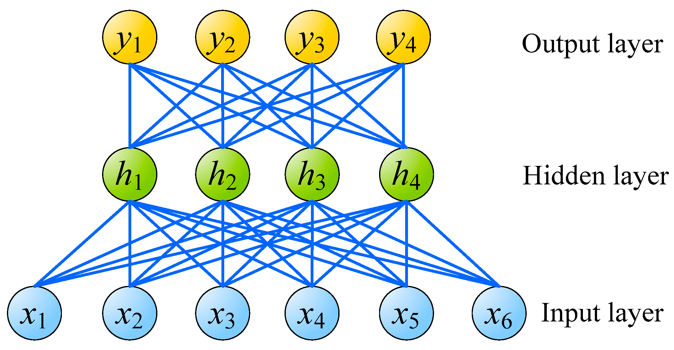
Artificial neural networks (ANNs) are computing systems inspired by the biological neural networks. The general structure of ANNs contains neurons, weights, and bias. Based on their powerful molding ability, ANNs are still very popular in the machine learning field. However, there are many ANN structures used in the machine learning problems, but the Multilayer Perceptron (MLP) [32] is the most commonly used ANN type. The MLP is a fully connected structure artificial neural network. The structure of MLP is shown in Figure 1. In general, the MLP consists of one input layer, one or more hidden layers, and one output layer. However, the MLP network presented in Figure 1 is the most common MLP structure, which has only one hidden layer. In the MLP, all the neurons of the previous layer are fully connected to the neurons of the next layer. In Figure 1, x1, x2, x3, … , x6 are the neurons of the input layer, h1, h2, h3, h4 are the neurons of the hidden layer, and y1, y2, y3, y4 are the neurons of the output layer. In the case of energy load forecasting, the input is the past energy load, and the output is the future energy load. Although, the MLP structure is very simple, it provides good results in many applications. The most commonly used algorithm for MLP training is the backpropagation algorithm.
Although MLPs are very good in modelling and patter recognition, the convolutional neural networks (CNNs) provide better accuracy in highly non-linear problems, such as energy load forecasting. The CNN uses the concept of weight sharing. The one-dimensional convolution and pooling layer are presented in Figure 2. The lines in the same color denote the same sharing weight, and sets of the sharing weights can be treated as kernels. After the convolution process, the inputs x1, x2, x3, … , x6 are transformed to the feature maps c1, c2, c3, c4. The next step in Figure 2 is pooling, wherein the feature map of convolution layer is sampled and its dimension is reduced. For instance, in Figure 2 dimension of the feature map is 4, and after pooling process that dimension is reduced to 2. The process of pooling is an important procedure to extract the important convolution features.
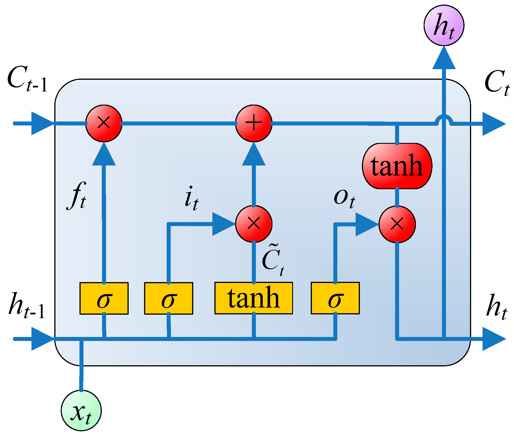
The other popular solution of the forecasting problem is Long Short Term Memory network (LSTM) [33]. The LSTM is a recurrent neural network, which has been used to solve many time sequence problems. The structure of LSTM is shown in Figure 3, and its operation is illustrated by the following equations:
where xt is the network input, and ht is the output of hidden layer, σ denotes the sigmoidal function, Ct is the cell state, and denotes the candidate value of the state. Besides, there are three gates in LSTM: it is the input gate, is the output gate, and ft is the forget gate. The LSTM is designed for solving the long-term dependency problem. In general, the LSTM provides good forecasting results.
3. The Proposed Deep Neural Network
The structure of the proposed deep neural network DeepEnergy is shown in Figure 4. Unlike the general forecasting method based on the LSTM, the DeepEnergy uses the CNN structure. The input layer denotes the information on past load, and the output values represent the future energy load. There are two main processes in DeepEnergy, feature extraction, and forecasting. The feature extraction in DeepEnergy is performed by three convolution layers (Conv1, Conv2, and Conv3) and three pooling layers (Pooling1, Pooling2, and Pooling3). The Conv1–Conv3 are one-dimensional (1D) convolutions, and the feature maps are all activated by the Rectified Linear Unit (ReLU) function. Besides, the kernel sizes of Conv1, Conv2, and Conv3 are 9, 5, 5, respectively, and the depths of the feature maps are 16, 32, 64, respectively. The pooling method of Pooling1 to Pooling3 is the max pooling, and the pooling size is equal to 2. Therefore, after the pooling process, the dimension of the feature map will be divided by 2 to extract the important features of the deeper layers.
In the forecasting, the first step is to flat the Pooling3 layer into one dimension and construct a fully connected structure between Flatten layer and Output layer. In order to fit the values previously normalized in the range [0, 1], the sigmoidal function is chosen as an activation function of the output layer. Furthermore, in order to overcome the overfitting problem, the dropout technology [34] is adopted in the fully connected layer. Namely, the dropout is an efficient way to prevent overfitting in artificial neural network. During the training process, neurons are randomly “dead”. As shown in Figure 4, the output values of chosen neurons (the gray circles) are equal to zero in certain training iteration. The chosen neurons are randomly changed during training process.
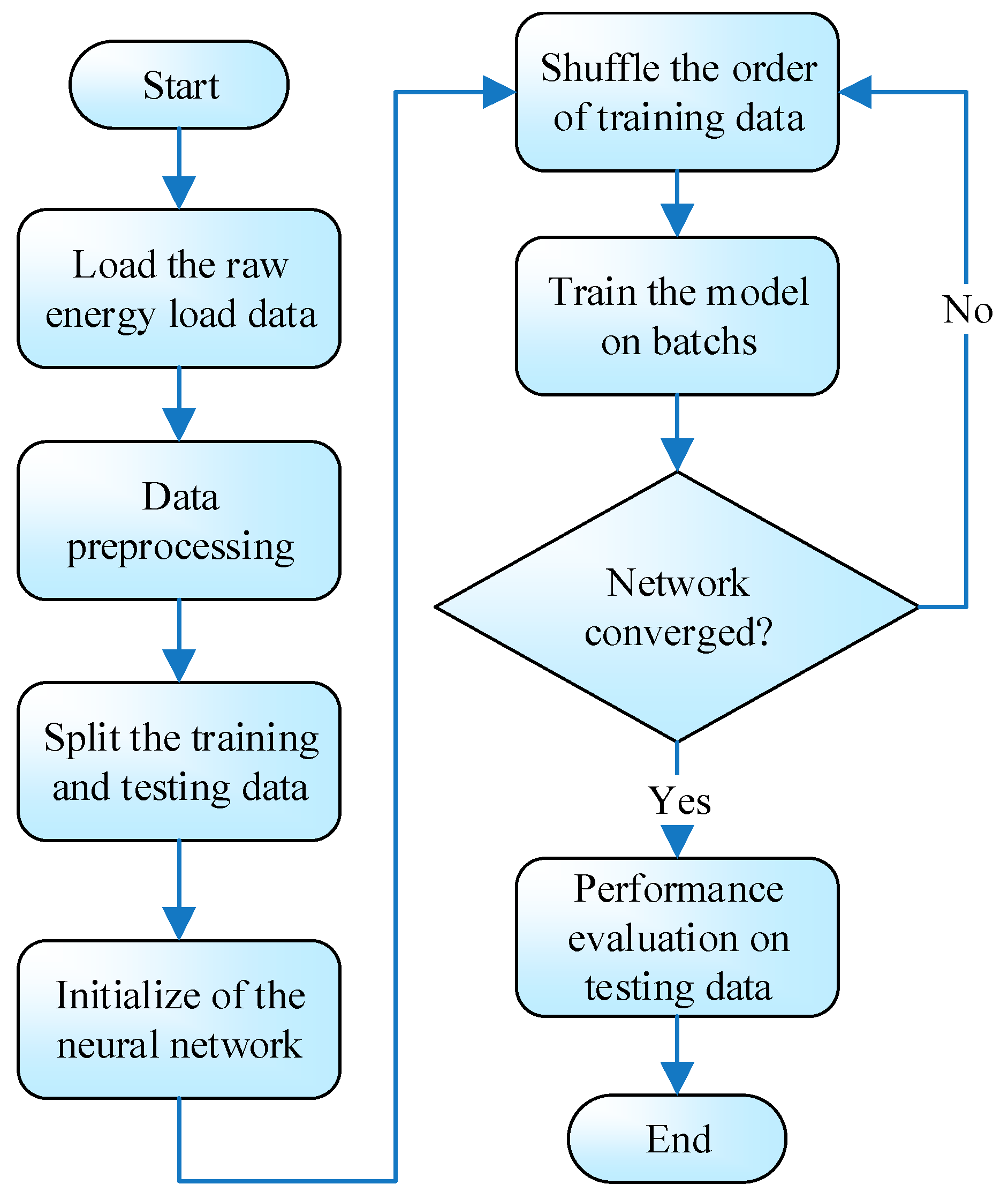
Furthermore, the flowchart of proposed DeepEnergy is represented in Figure 5. Firstly, the raw energy load data are loaded into the memory. Then, the data preprocessing is executed and data are normalized in the range [0, 1] in order to fit the characteristic of the machine learning model. For the purpose of validation of DeepEnergy generalization performance, the data are split into training data and testing data. The training data are used for training of proposed model. After the training process, the proposed DeepEnergy network is created and initialized. Before the training, the training data are randomly shuffled to force the proposed model to learn complicated relationships between input and output data. The training data are split into several batches. According to the order of shuffled data, the model is trained on all of the batches. During the training process, if the desired Mean Square Error (MSE) is not reached in the current epoch, the training will continue until the maximal number of epochs or desired MSE is reached. On the contrary, if the maximal number of epochs is reached, then the training process will stop regardless the MSE value. Final performances are evaluated to demonstrate feasibility and practicability of the proposed method.
4. Experimental Results
In the experiment, the USA District public consumption dataset and electric load dataset from 2016 provided by the Electric Reliability Council of Texas were used. Since then, the support vector machine (SVM) [35] is a popular machine learning technology, in experiment; the radial basis function (RBF) kernels of SVM were chosen to demonstrate the SVM performance. Besides, the random forest (RF) [36], decision tree (DT) [37], MLP, LSTM, and proposed DeepEnergy network were also implemented and tested. The results of load forecasting by all of the methods are shown in Figure 6, Figure 7, Figure 8, Figure 9, Figure 10 and Figure 11. In the experiment, the training data were two-month data, and test data were one-month data. In order to evaluate the performances of all listed methods, the dataset was divided into 10 partitions. In the first partition, training data consisted of energy load data collected in January and February 2016, and test data consisted of data collected in March 2016. In the second partition, training data were data collected in February and March 2016, and test data were data collected in April 2016. The following partitions can be deduced by the same analogy.
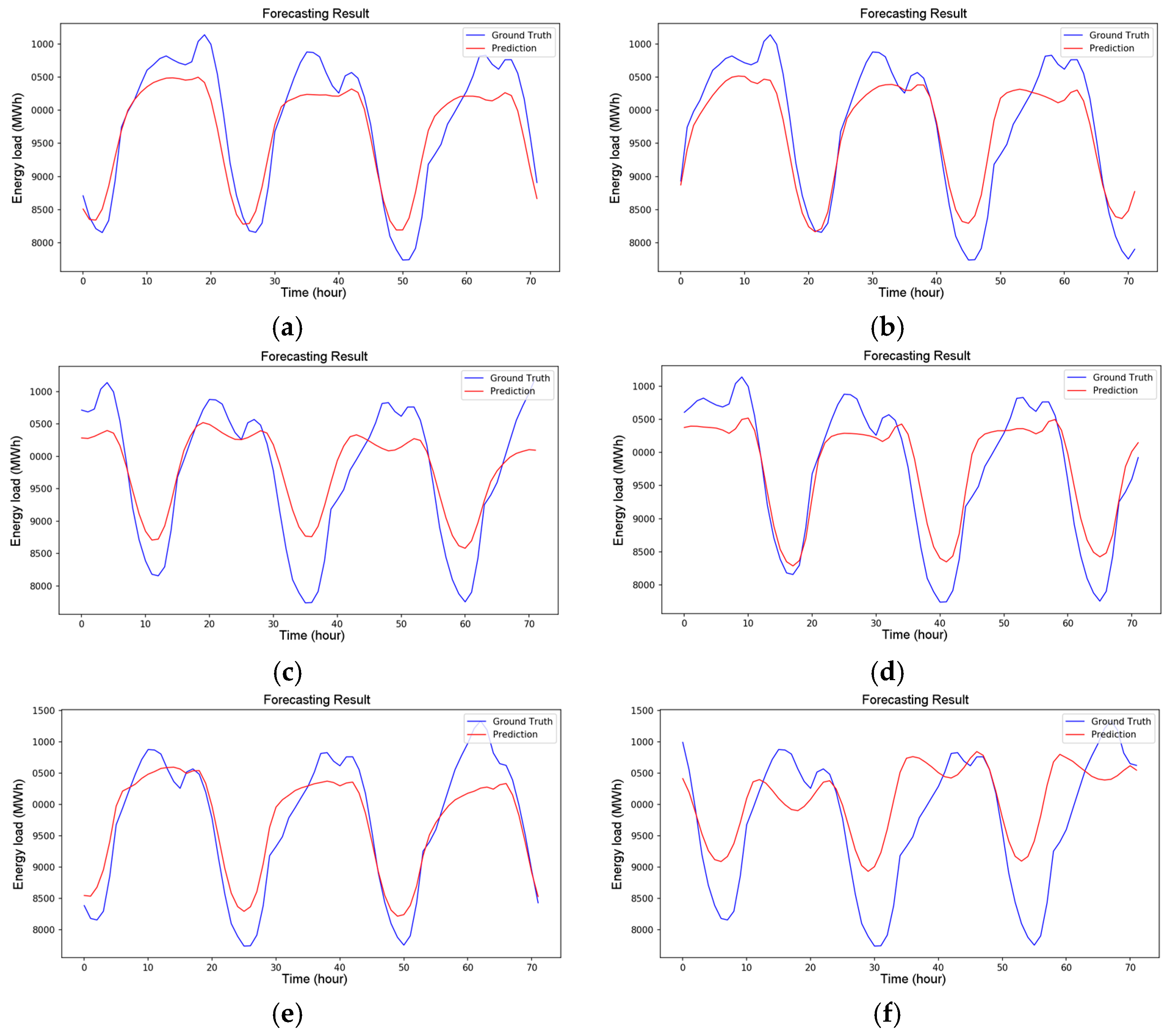
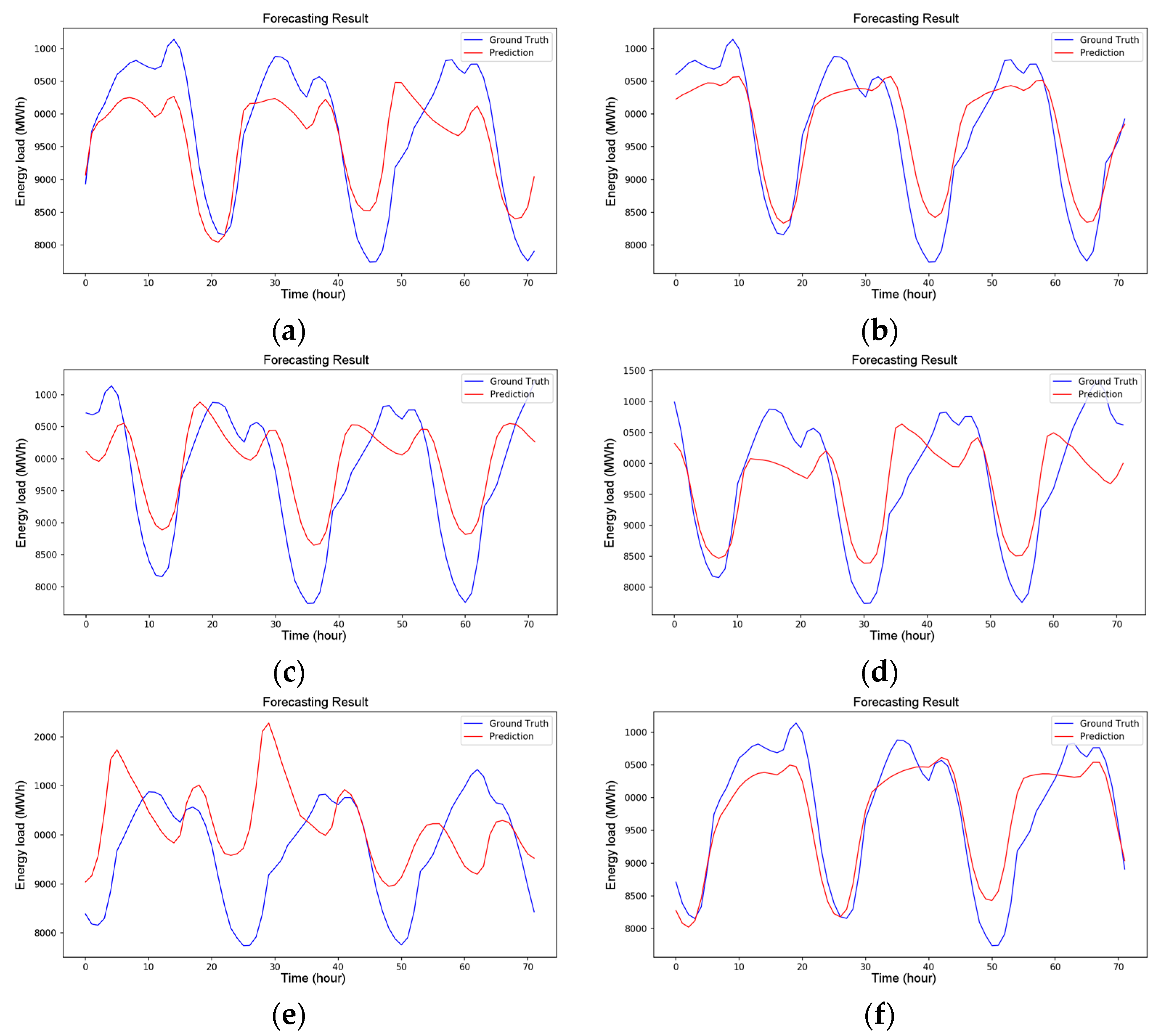
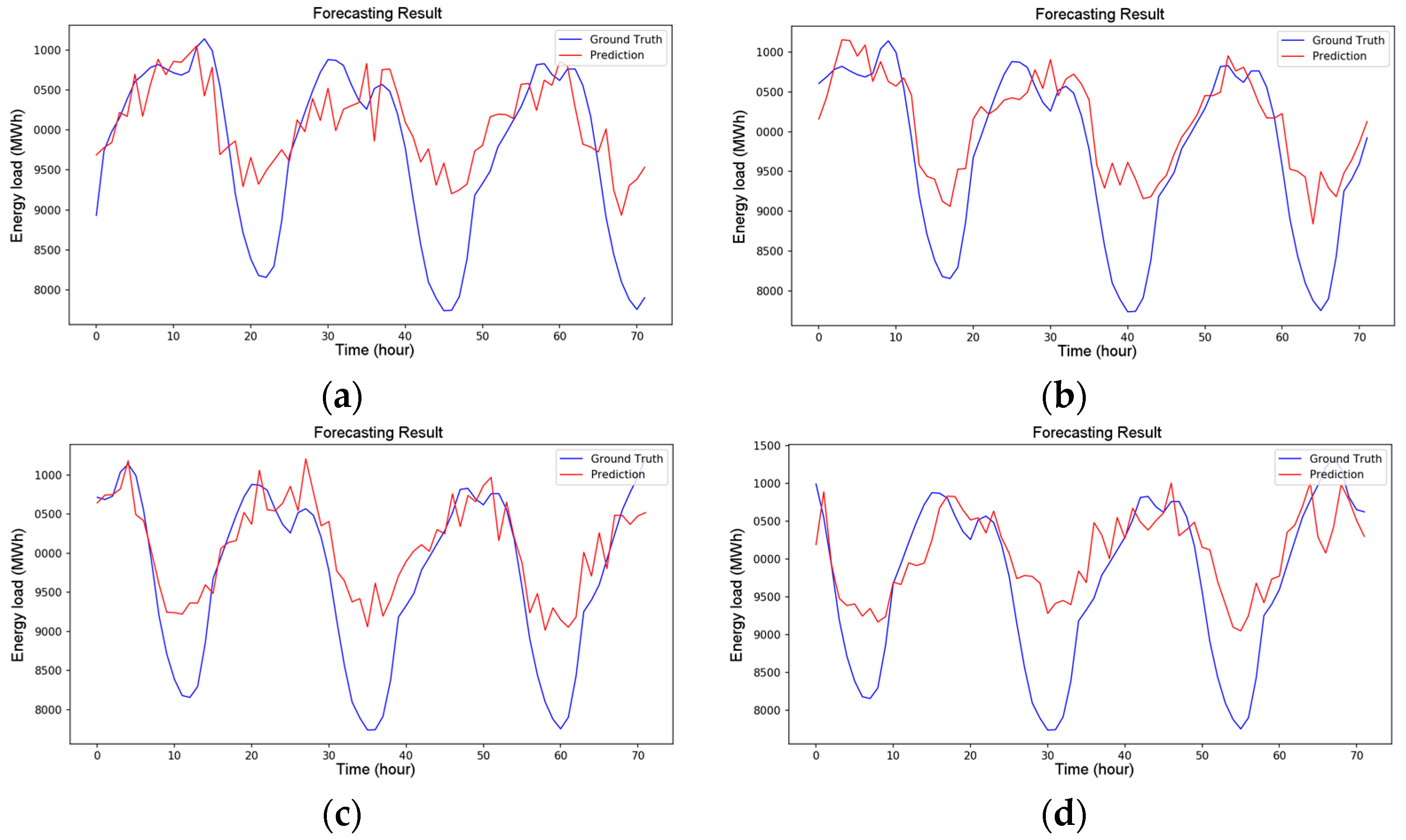
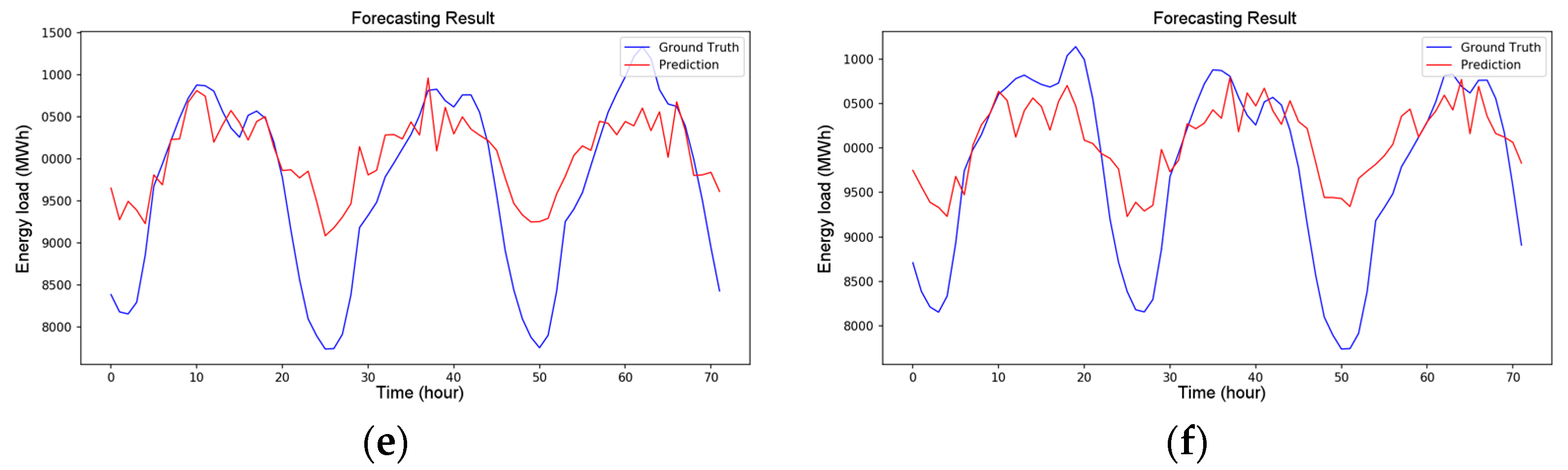
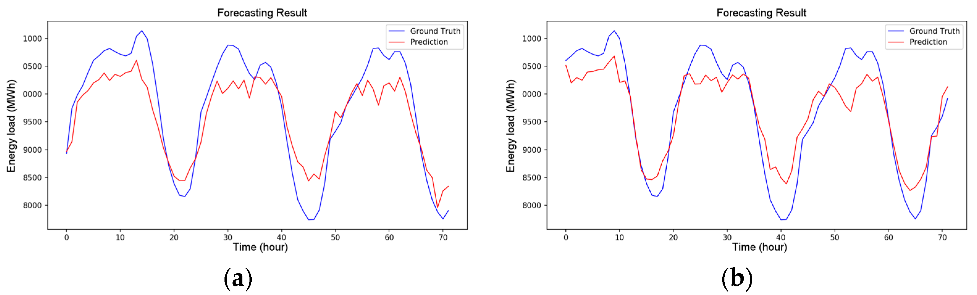
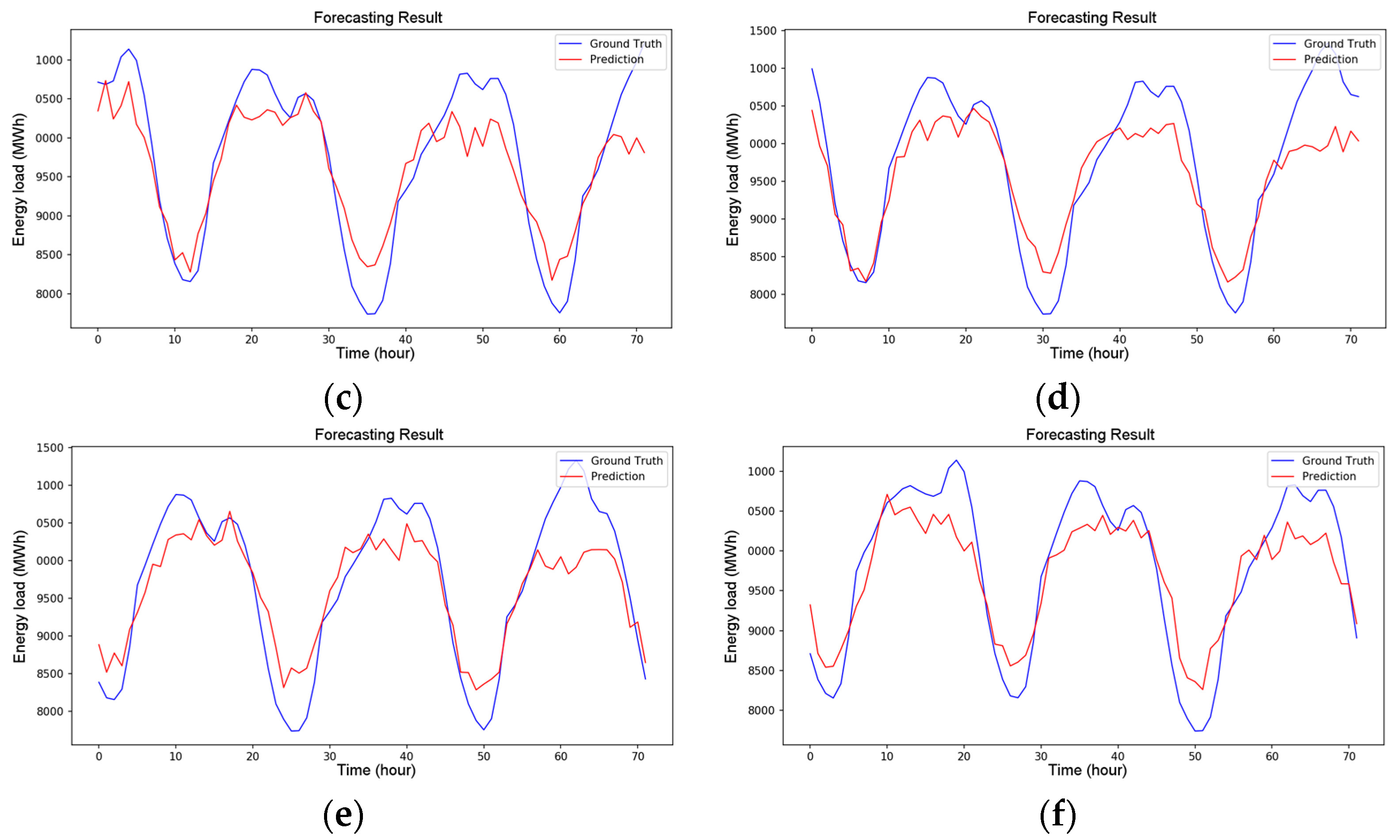
In Figure 6, Figure 7, Figure 8, Figure 9, Figure 10 and Figure 11, red curves denote the forecasting results of the corresponding models, and blue curves represent the ground truth. The vertical axes represent the energy load (MWh), and the horizontal axes denote the time (hour). The energy load from the past (24 × 7) h was used as an input of the forecasting model, and predicted energy load in the next (24 × 3) h was an output of the forecasting model. After the models received the past (24 × 7) h data, they forecasted the next (24 × 3) h energy load, red curves in Figure 6, Figure 7, Figure 8, Figure 9, Figure 10 and Figure 11. Besides, the correct information is illustrated by blue curves. The differences between red and blue curves denote the performances of the corresponding models. For the sake of comparison fairness, testing data were not used during the training process of models. According to the results presented in Figure 6, Figure 7, Figure 8, Figure 9, Figure 10 and Figure 11, the proposed DeepEnergy network has the best prediction performance among all of the models.
In order to evaluate the performance of forecasting models more accurately, the Mean Absolute Percentage Error (MAPE) and Cumulative Variation of Root Mean Square Error (CV-RMSE) were employed. The MAPE and CV-RMSE are defined by Equations (7) and (8), respectively, where yn denotes the measured value, is the estimated value, and N represents the sample size.
The detailed experimental results are presented numerically in Table 1 and Table 2. As shown in Table 1 and Table 2, the MAPE and CV-RMSE of the DeepEnergy model are the smallest and the goodness of error is the best among all models, namely, average MAPE and CV-RMSE are 9.77% and 11.65%, respectively. The MAPE of MLP model is the largest among all of the models; an average error is about 15.47%. On the other hand, the CV-RMSE of SVM model is the largest among all models; an average error is about 17.47%. According to the average MAPE and CV-RMSE values, the electric load forecasting accuracy of tested models in descending order is as follows: DeepEnergy, RF, LSTM, DT, SVM, and MLP.
It is obvious that red curve in Figure 11, which denotes the DeepEnergy algorithm, is better than other curves in Figure 6, Figure 7, Figure 8, Figure 9 and Figure 10, which further verifies that the proposed DeepEnergy algorithm has the best prediction performance. Therefore, it is proven that the DeepEnergy STLF algorithm proposed in the paper is practical and effective. Although the LSTM has good performance in time sequence problems, in this study, the reduction of training loss is still not fast enough to handle this forecasting problem because the size of input and output data is too large for the traditional LSTM neural network. Therefore, the traditional LSTM is not suitable for this kind of prediction. Finally, the experimental results show that proposed DeepEnergy network provides the best results in energy load forecasting.
5. Discussion
The traditional machine learning methods, such as SVM, random forest, and decision tree, are widely used in many applications. In this study, these methods also provide acceptable results. In aspect of SVM, the supporting vectors are mapped into a higher dimensional space by the kernel function. Therefore, the selection of kernel function is very important. In order to achieve the goal of nonlinear energy load forecasting, the RBF is chosen as a SVM kernel. When compared with the SVM, the learning concept of decision tree is much simpler. Namely, the decision tree is a flowchart structure easy to understand and interpret. However, only one decision tree does not have the ability to solve complicated problems. Therefore, the random forest, which represents the combination of numerous decision trees, provides the model ensemble solution. In this paper, the experimental results of random forest are better than those of decision tree and SVM, which proves that the model ensemble solution is effective in the energy load forecasting. In aspect of the neural networks, the MLP is the simplest ANN structure. Although the MLP can model the nonlinear energy forecasting task, its performance in this experiment is not outstanding. On the other hand, the LSTM considers data relationships in time steps during the training. According to the result, the LSTM can deal with the time sequence problems, and the forecasting trend is marginally correct. However, the proposed CNN structure, named the DeepEnergy, has the best results in the experiment. The experiments demonstrate that the most important feature can be extracted by the designed 1D convolution and pooling layers. This verification also proves the CNN structure is effective in the forecasting, and the proposed DeepEnergy gives the outstanding results. This paper not only provides the comparison of the traditional machine learning and deep learning methods, but also gives a new research direction in the energy load forecasting.
6. Conclusions
This paper proposes a powerful deep convolutional neural network model (DeepEnergy) for energy load forecasting. The proposed network is validated by experiment with the load data from the past seven days. In the experiment, the data from coast area of the USA were used and historical electricity demand from consumers was considered. According to the experimental results, the DeepEnergy can precisely predict energy load in the next three days. In addition, the proposed algorithm was compared with five AI algorithms that were commonly used in load forecasting. The comparison showed that performance of DeepEnergy was the best among all tested algorithms, namely the DeepEnergy had the lowest values of both MAPE and CV-RMSE. According to all of the obtained results, the proposed method can reduce monitoring expenses, initial cost of hardware components, and long-term maintenance costs in the future smart grids. Simultaneously, the results verify that proposed DeepEnergy STLF method has strong generalization ability and robustness, thus it can achieve very good forecasting performance.
Acknowledgments
This work was supported by the Ministry of Science and Technology, Taiwan, Republic of China, under Grants MOST 106-2218-E-153-001-MY3.
Author Contributions
Ping-Huan Kuo wrote the program and designed the DNN model. Chiou-Jye Huang planned this study and collected the energy load dataset. Ping-Huan Kuo and Chiou-Jye Huang contributed in drafted and revised manuscript.
Conflicts of Interest
The authors declare no conflict of interest.
References
- Raza, M.Q.; Khosravi, A. A review on artificial intelligence based load demand forecasting techniques for smart grid and buildings. Renew. Sustain. Energy Rev. 2015, 50, 1352–1372. [Google Scholar] [CrossRef]
- Da Graça Carvalho, M.; Bonifacio, M.; Dechamps, P. Building a low carbon society. Energy 2011, 36, 1842–1847. [Google Scholar] [CrossRef]
- Jiang, B.; Sun, Z.; Liu, M. China’s energy development strategy under the low-carbon economy. Energy 2010, 35, 4257–4264. [Google Scholar] [CrossRef]
- Cho, H.; Goude, Y.; Brossat, X.; Yao, Q. Modeling and forecasting daily electricity load curves: A hybrid approach. J. Am. Stat. Assoc. 2013, 108, 7–21. [Google Scholar] [CrossRef] [Green Version]
- Javed, F.; Arshad, N.; Wallin, F.; Vassileva, I.; Dahlquist, E. Forecasting for demand response in smart grids: An analysis on use of anthropologic and structural data and short term multiple loads forecasting. Appl. Energy 2012, 96, 150–160. [Google Scholar] [CrossRef]
- Iwafune, Y.; Yagita, Y.; Ikegami, T.; Ogimoto, K. Short-term forecasting of residential building load for distributed energy management. In Proceedings of the 2014 IEEE International Energy Conference, Cavtat, Croatia, 13–16 May 2014; pp. 1197–1204. [Google Scholar] [CrossRef]
- Short Term Electricity Load Forecasting on Varying Levels of Aggregation. Available online: https://arxiv.org/abs/1404.0058v3 (accessed on 11 January 2018).
- Gerwig, C. Short term load forecasting for residential buildings—An extensive literature review. Smart Innov. Syst. 2015, 39, 181–193. [Google Scholar]
- Hippert, H.S.; Pedreira, C.E.; Souza, R.C. Neural networks for short-term load forecasting: A review and evaluation. IEEE Trans. Power Syst. 2001, 16, 44–55. [Google Scholar] [CrossRef]
- Metaxiotis, K.; Kagiannas, A.; Askounis, D.; Psarras, J. Artificial intelligence in short term electric load forecasting: A state-of-the-art survey for the researcher. Energy Convers. Manag. 2003, 44, 1524–1534. [Google Scholar] [CrossRef]
- Tzafestas, S.; Tzafestas, E. Computational intelligence techniques for short-term electric load forecasting. J. Intell. Robot. Syst. 2001, 31, 7–68. [Google Scholar] [CrossRef]
- Ghayekhloo, M.; Menhaj, M.B.; Ghofrani, M. A hybrid short-term load forecasting with a new data preprocessing framework. Electr. Power Syst. Res. 2015, 119, 138–148. [Google Scholar] [CrossRef]
- Xia, C.; Wang, J.; McMenemy, K. Short, medium and long term load forecasting model and virtual load forecaster based on radial basis function neural networks. Int. J. Electr. Power Energy Syst. 2010, 32, 743–750. [Google Scholar] [CrossRef] [Green Version]
- Bughin, J.; Hazan, E.; Ramaswamy, S.; Chui, M. Artificial Intelligence—The Next Digital Frontier? Mckinsey Global Institute: New York, NY, USA, 2017; pp. 1–80. [Google Scholar]
- Oh, C.; Lee, T.; Kim, Y.; Park, S.; Kwon, S.B.; Suh, B. Us vs. Them: Understanding Artificial Intelligence Technophobia over the Google DeepMind Challenge Match. In Proceedings of the 2017 CHI Conference on Human Factors in Computing Systems, Denver, CO, USA, 6–11 May 2017; pp. 2523–2534. [Google Scholar] [CrossRef]
- Skilton, M.; Hovsepian, F. Example Case Studies of Impact of Artificial Intelligence on Jobs and Productivity. In 4th Industrial Revolution; National Academies Press: Washingtom, DC, USA, 2018; pp. 269–291. [Google Scholar]
- Ekonomou, L.; Christodoulou, C.A.; Mladenov, V. A short-term load forecasting method using artificial neural networks and wavelet analysis. Int. J. Power Syst. 2016, 1, 64–68. [Google Scholar]
- Valgaev, O.; Kupzog, F. Low-Voltage Power Demand Forecasting Using K-Nearest Neighbors Approach. In Proceedings of the Innovative Smart Grid Technologies—Asia (ISGT-Asia), Melbourne, VIC, Australia, 28 November–1 December 2016. [Google Scholar]
- Valgaev, O.; Kupzog, F. Building Power Demand Forecasting Using K-Nearest Neighbors Model—Initial Approach. In Proceedings of the IEEE PES Asia-Pacific Power Energy Conference, Xi’an, China, 25–28 October 2016; pp. 1055–1060. [Google Scholar]
- Humeau, S.; Wijaya, T.K.; Vasirani, M.; Aberer, K. Electricity load forecasting for residential customers: Exploiting aggregation and correlation between households. In Proceedings of the 2013 Sustainable Internet and ICT for Sustainability, Palermo, Italy, 30–31 October 2013. [Google Scholar]
- Veit, A.; Goebel, C.; Tidke, R.; Doblander, C.; Jacobsen, H. Household electricity demand forecasting: Benchmarking state-of-the-art method. In Proceedings of the 5th International Confrerence Future Energy Systems, Cambridge, UK, 11–13 June 2014; pp. 233–234. [Google Scholar] [CrossRef]
- Jetcheva, J.G.; Majidpour, M.; Chen, W. Neural network model ensembles for building-level electricity load forecasts. Energy Build. 2014, 84, 214–223. [Google Scholar] [CrossRef]
- Kardakos, E.G.; Alexiadis, M.C.; Vagropoulos, S.I.; Simoglou, C.K.; Biskas, P.N.; Bakirtzis, A.G. Application of time series and artificial neural network models in short-term forecasting of PV power generation. In Proceedings of the 2013 48th International Universities’ Power Engineering Conference, Dublin, Ireland, 2–5 September 2013; pp. 1–6. [Google Scholar] [CrossRef]
- Fujimoto, Y.; Hayashi, Y. Pattern sequence-based energy demand forecast using photovoltaic energy records. In Proceedings of the 2012 International Conference on Renewable Energy Research and Applications, Nagasaki, Japan, 11–14 November 2012. [Google Scholar]
- Chaouch, M. Clustering-based improvement of nonparametric functional time series forecasting: Application to intra-day household-level load curves. IEEE Trans. Smart Grid 2014, 5, 411–419. [Google Scholar] [CrossRef]
- Niu, D.; Dai, S. A short-term load forecasting model with a modified particle swarm optimization algorithm and least squares support vector machine based on the denoising method of empirical mode decomposition and grey relational analysis. Energies 2017, 10, 408. [Google Scholar] [CrossRef]
- Deo, R.C.; Wen, X.; Qi, F. A wavelet-coupled support vector machine model for forecasting global incident solar radiation using limited meteorological dataset. Appl. Energy 2016, 168, 568–593. [Google Scholar] [CrossRef]
- Soubdhan, T.; Ndong, J.; Ould-Baba, H.; Do, M.T. A robust forecasting framework based on the Kalman filtering approach with a twofold parameter tuning procedure: Application to solar and photovoltaic prediction. Sol. Energy 2016, 131, 246–259. [Google Scholar] [CrossRef]
- Hahn, H.; Meyer-Nieberg, S.; Pickl, S. Electric load forecasting methods: Tools for decision making. Eur. J. Oper. Res. 2009, 199, 902–907. [Google Scholar] [CrossRef]
- Zhang, G.; Patuwo, B.E.; Hu, M.Y. Forecasting with artificial neural networks: The state of the art. Int. J. Forecast. 1998, 14, 35–62. [Google Scholar] [CrossRef]
- Pappas, S.S.; Ekonomou, L.; Moussas, V.C.; Karampelas, P.; Katsikas, S.K. Adaptive load forecasting of the Hellenic electric grid. J. Zhejiang Univ. A 2008, 9, 1724–1730. [Google Scholar] [CrossRef]
- White, B.W.; Rosenblatt, F. Principles of neurodynamics: Perceptrons and the theory of brain mechanisms. Am. J. Psychol. 1963, 76, 705. [Google Scholar] [CrossRef]
- Hochreiter, S.; Urgen Schmidhuber, J. Long short-term memory. Neural Comput. 1997, 9, 1735–1780. [Google Scholar] [CrossRef] [PubMed]
- Srivastava, N.; Hinton, G.; Krizhevsky, A.; Sutskever, I.; Salakhutdinov, R. Dropout: A Simple Way to Prevent Neural Networks from Overfitting. J. Mach. Learn. Res. 2014, 15, 1929–1958. [Google Scholar] [CrossRef]
- Suykens, J.A.K.; Vandewalle, J. Least squares support vector machine classifiers. Neural Process. Lett. 1999, 9, 293–300. [Google Scholar] [CrossRef]
- Liaw, A.; Wiener, M. Classification and Regression by randomForest. R News 2002, 2, 18–22. [Google Scholar] [CrossRef]
- Safavian, S.R.; Landgrebe, D. A Survey of Decision Tree Classifier Methodology. IEEE Trans. Syst. Man Cybern. 1991, 21, 660–674. [Google Scholar] [CrossRef]
Figure 1.
The Multilayer Perceptron (MLP) structure.

Figure 2.
The one-dimensional (1D) convolution and pooling layer.

Figure 3.
The Long Short Term Memory network (LSTM) structure.

Figure 4.
The DeepEnergy structure.

Figure 5.
The DeepEnergy flowchart.

Figure 6.
The forecasting results of support vector machine (SVM): (a) Partial results A; (b) Partial results B; (c) Partial results C; (d) Partial results D; (e) Partial results E; (f) Partial results F.
Figure 6.
The forecasting results of support vector machine (SVM): (a) Partial results A; (b) Partial results B; (c) Partial results C; (d) Partial results D; (e) Partial results E; (f) Partial results F.

Figure 7.
The forecasting results of random forest (RF): (a) Partial results A; (b) Partial results B; (c) Partial results C; (d) Partial results D; (e) Partial results E; (f) Partial results F.
Figure 7.
The forecasting results of random forest (RF): (a) Partial results A; (b) Partial results B; (c) Partial results C; (d) Partial results D; (e) Partial results E; (f) Partial results F.

Figure 8.
The forecasting results of decision tree (DT): (a) Partial results A; (b) Partial results B; (c) Partial results C; (d) Partial results D; (e) Partial results E; (f) Partial results F.
Figure 8.
The forecasting results of decision tree (DT): (a) Partial results A; (b) Partial results B; (c) Partial results C; (d) Partial results D; (e) Partial results E; (f) Partial results F.

Figure 9.
The forecasting results of Multilayer Perceptron (MLP): (a) Partial results A; (b) Partial results B; (c) Partial results C; (d) Partial results D; (e) Partial results E; (f) Partial results F.
Figure 9.
The forecasting results of Multilayer Perceptron (MLP): (a) Partial results A; (b) Partial results B; (c) Partial results C; (d) Partial results D; (e) Partial results E; (f) Partial results F.


Figure 10.
The forecasting results of LSTM: (a) Partial results A; (b) Partial results B; (c) Partial results C; (d) Partial results D; (e) Partial results E; (f) Partial results F.
Figure 10.
The forecasting results of LSTM: (a) Partial results A; (b) Partial results B; (c) Partial results C; (d) Partial results D; (e) Partial results E; (f) Partial results F.

Figure 11.
The forecasting results of proposed DeepEnergy: (a) Partial results A; (b) Partial results B; (c) Partial results C; (d) Partial results D; (e) Partial results E; (f) Partial results F.
Figure 11.
The forecasting results of proposed DeepEnergy: (a) Partial results A; (b) Partial results B; (c) Partial results C; (d) Partial results D; (e) Partial results E; (f) Partial results F.


Table 1.
The experimental results in terms of Mean Absolute Percentage Error (MAPE) given in percentages.
Table 1.
The experimental results in terms of Mean Absolute Percentage Error (MAPE) given in percentages.
| Test | SVM | RF | DT | MLP | LSTM | DeepEnergy |
|---|---|---|---|---|---|---|
| #1 | 7.327408 | 7.639133 | 8.46043 | 9.164315 | 10.40804813 | 7.226127 |
| #2 | 7.550818 | 8.196129 | 10.23476 | 11.14954 | 9.970662683 | 8.244051 |
| #3 | 13.07929 | 10.11102 | 12.14039 | 19.99848 | 14.85568499 | 11.00656 |
| #4 | 16.15765 | 17.27957 | 19.86511 | 22.45493 | 12.83487893 | 12.17574 |
| #5 | 5.183255 | 6.570061 | 8.50582 | 15.01856 | 5.479091542 | 5.41808 |
| #6 | 10.33686 | 9.944028 | 11.11948 | 10.94331 | 11.7681534 | 9.070998 |
| #7 | 8.934657 | 6.698508 | 8.634132 | 7.722149 | 7.583802292 | 9.275215 |
| #8 | 18.5432 | 16.09926 | 17.17215 | 16.93843 | 15.6574951 | 13.2776 |
| #9 | 49.97551 | 17.9049 | 21.29354 | 29.06767 | 16.31443679 | 11.18214 |
| #10 | 11.20804 | 8.221766 | 10.68665 | 12.20551 | 8.390061493 | 10.80571 |
| Average | 14.82967 | 10.86644 | 12.81125 | 15.46629 | 11.32623153 | 9.768222 |
Table 2.
The experimental results in terms of Cumulative Variation of Root Mean Square Error (CV-RMSE) given in percentages.
Table 2.
The experimental results in terms of Cumulative Variation of Root Mean Square Error (CV-RMSE) given in percentages.
| Test | SVM | RF | DT | MLP | LSTM | DeepEnergy |
|---|---|---|---|---|---|---|
| #1 | 9.058992 | 9.423908 | 10.57686 | 10.65546 | 12.16246177 | 8.948922 |
| #2 | 10.14701 | 10.63412 | 12.99834 | 13.91199 | 12.19377007 | 10.46165 |
| #3 | 17.02552 | 12.42314 | 14.58249 | 23.2753 | 16.9291218 | 13.30116 |
| #4 | 21.22162 | 21.1038 | 24.48298 | 23.63544 | 14.13596516 | 14.63439 |
| #5 | 6.690527 | 7.942747 | 10.10017 | 15.44461 | 6.334195125 | 6.653999 |
| #6 | 11.88856 | 11.6989 | 13.39033 | 12.20149 | 12.96057349 | 10.74021 |
| #7 | 10.77881 | 7.871596 | 10.35254 | 8.716806 | 8.681353107 | 10.85454 |
| #8 | 19.49707 | 17.09079 | 18.95726 | 17.73124 | 16.55737557 | 14.51027 |
| #9 | 54.58171 | 19.91185 | 24.84425 | 29.37466 | 17.66342548 | 13.01906 |
| #10 | 13.80167 | 10.15117 | 13.06351 | 13.39278 | 10.20235927 | 13.47003 |
| Average | 17.46915 | 12.8252 | 15.33487 | 16.83398 | 12.78206008 | 11.65942 |
© 2018 by the authors. Licensee MDPI, Basel, Switzerland. This article is an open access article distributed under the terms and conditions of the Creative Commons Attribution (CC BY) license (http://creativecommons.org/licenses/by/4.0/).
Share and Cite
MDPI and ACS Style
Kuo, P.-H.; Huang, C.-J. A High Precision Artificial Neural Networks Model for Short-Term Energy Load Forecasting. Energies 2018, 11, 213. https://doi.org/10.3390/en11010213
AMA Style
Kuo P-H, Huang C-J. A High Precision Artificial Neural Networks Model for Short-Term Energy Load Forecasting. Energies. 2018; 11(1):213. https://doi.org/10.3390/en11010213
Chicago/Turabian StyleKuo, Ping-Huan, and Chiou-Jye Huang. 2018. "A High Precision Artificial Neural Networks Model for Short-Term Energy Load Forecasting" Energies 11, no. 1: 213. https://doi.org/10.3390/en11010213
Note that from the first issue of 2016, this journal uses article numbers instead of page numbers. See further details here.