Big Data Mining of Energy Time Series for Behavioral Analytics and Energy Consumption Forecasting


Department of Software Engineering at Lakehead Univerity, Thunder Bay, ON, P7B 5E1, Canada
*
Author to whom correspondence should be addressed.
Energies 2018, 11(2), 452; https://doi.org/10.3390/en11020452
Submission received: 24 December 2017
/
Revised: 10 February 2018
/
Accepted: 12 February 2018
/
Published: 20 February 2018
(This article belongs to the Special Issue Data Science and Big Data in Energy Forecasting)
Abstract
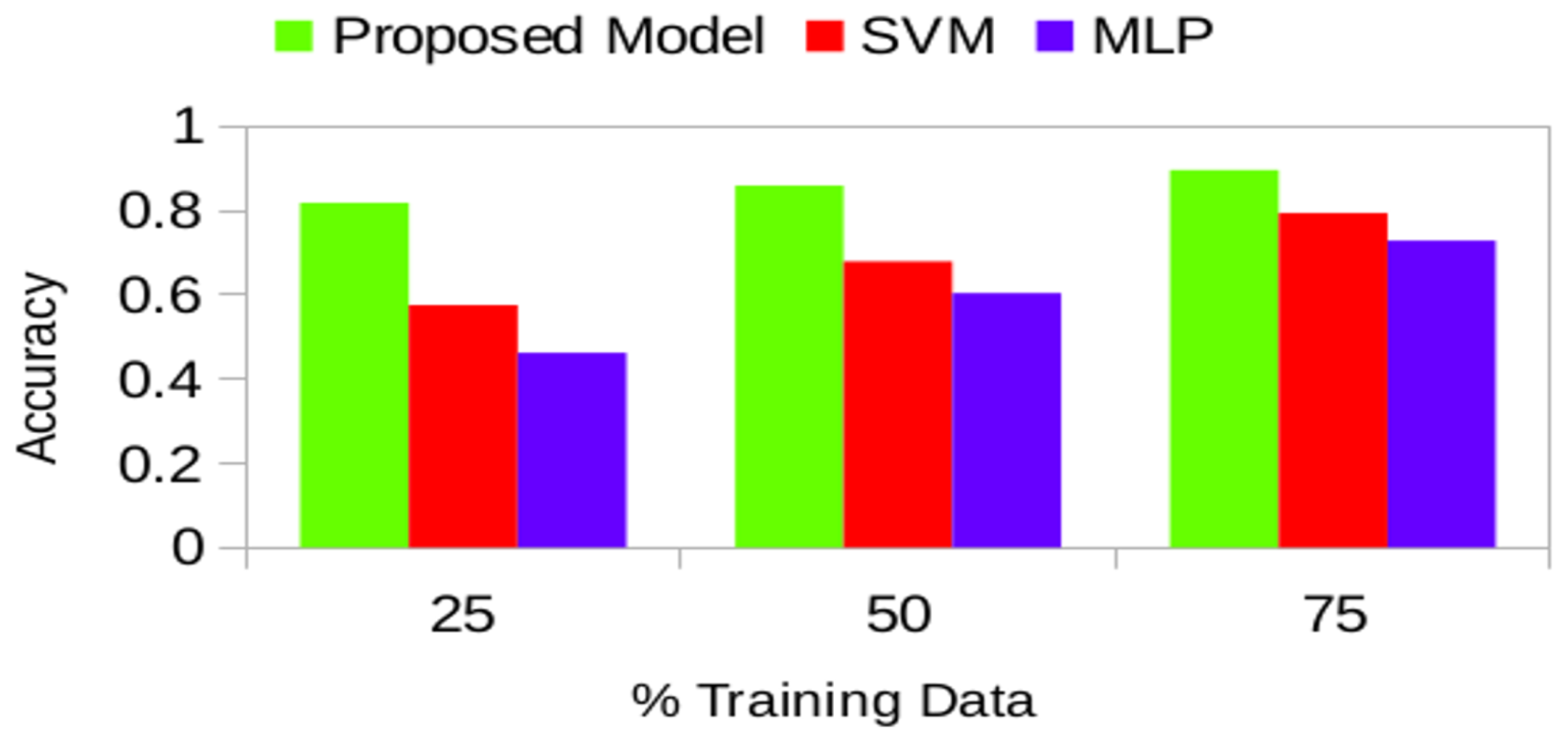
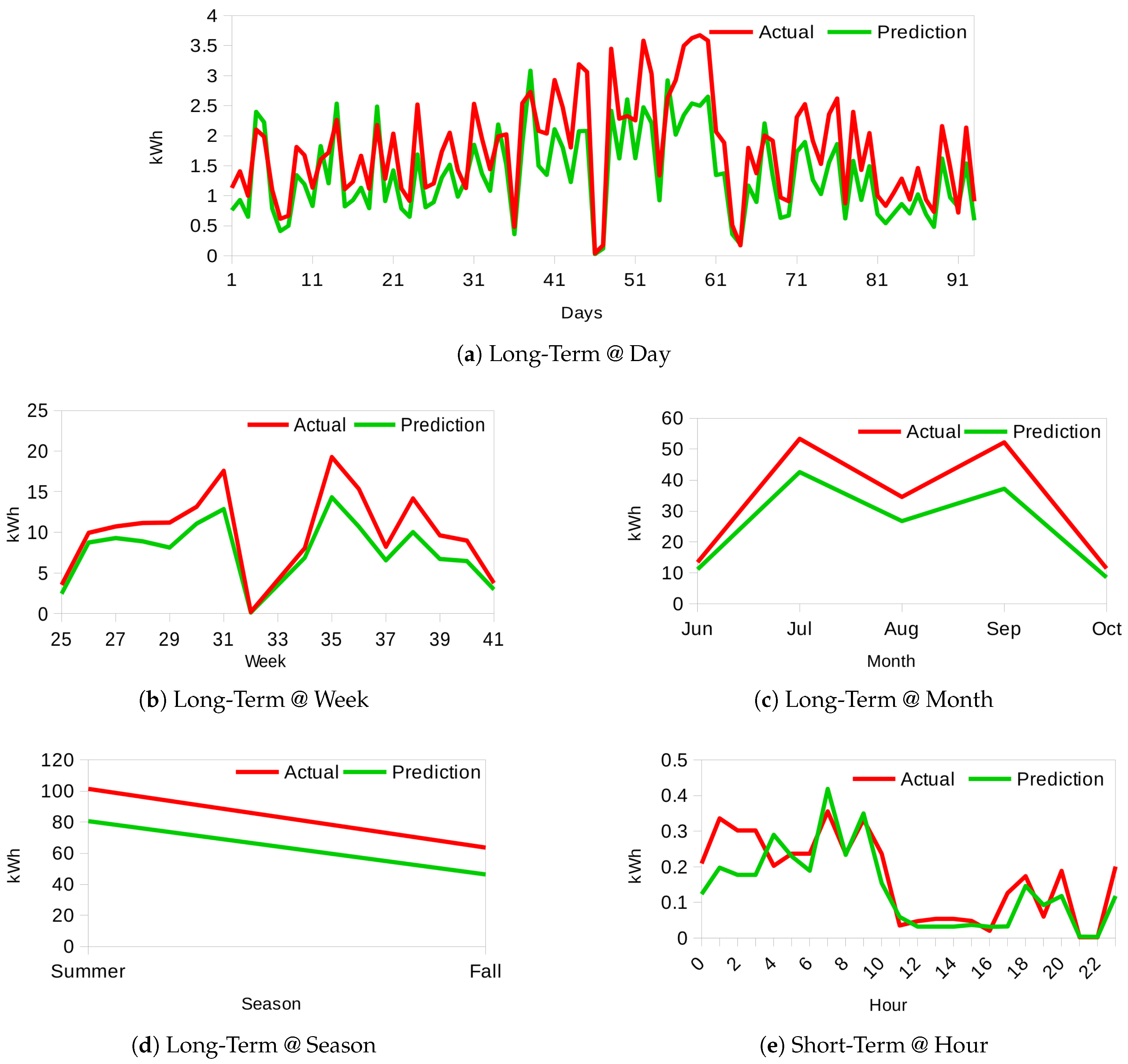
:Responsible, efficient and environmentally aware energy consumption behavior is becoming a necessity for the reliable modern electricity grid. In this paper, we present an intelligent data mining model to analyze, forecast and visualize energy time series to uncover various temporal energy consumption patterns. These patterns define the appliance usage in terms of association with time such as hour of the day, period of the day, weekday, week, month and season of the year as well as appliance-appliance associations in a household, which are key factors to infer and analyze the impact of consumers’ energy consumption behavior and energy forecasting trend. This is challenging since it is not trivial to determine the multiple relationships among different appliances usage from concurrent streams of data. Also, it is difficult to derive accurate relationships between interval-based events where multiple appliance usages persist for some duration. To overcome these challenges, we propose unsupervised data clustering and frequent pattern mining analysis on energy time series, and Bayesian network prediction for energy usage forecasting. We perform extensive experiments using real-world context-rich smart meter datasets. The accuracy results of identifying appliance usage patterns using the proposed model outperformed Support Vector Machine (SVM) and Multi-Layer Perceptron (MLP) at each stage while attaining a combined accuracy of 81.82%, 85.90%, 89.58% for 25%, 50% and 75% of the training data size respectively. Moreover, we achieved energy consumption forecast accuracies of 81.89% for short-term (hourly) and 75.88%, 79.23%, 74.74%, and 72.81% for the long-term; i.e., day, week, month, and season respectively.
1. Introduction
Currently, smart meters are being deployed in millions of houses, offering bidirectional communication between the consumers and the utility companies; which has given rise to a pervasive computing environment generating extensive volumes of data with high velocity and veracity attributes. Such data have a time-series notion typically consisting of energy usage measurements of component appliances over a time interval [1]. The advent of big data technologies, capable of ingesting this large volume of time series streams and facilitating data-driven decision making through transforming data into actionable insights, can revolutionize utility providers’ capabilities for learning customer energy usage patterns, forecasting demand, preventing outages, and optimizing energy usage.
Utility companies are constantly working towards determining the best ways to reduce cost and improve profitability by introducing programs, such as demand-side management and demand response, that best fit the consumers’ energy consumption profiles. Although there has been a marginal success in achieving the goals of such programs, sustainable results are yet to be accomplished [2]. This is because it is a challenging to understand consumers’ habits individually and tailor strategies that take into account the benefits vs. discomfort from modifying behavior according to suggested energy-saving plans. Furthermore, the relationship between human behavior and the parameters affecting energy consumption patterns are non-static [2]. Consumer behavior is dependent on weather and seasons and has a variable influence on energy consumption decisions. Thereby, actively engaging consumers in personalized energy management by facilitating well-timed feedback on energy consumption and related cost is key to steering suitable energy saving schemes or programs [3]. Therefore, designing models that are capable of analyzing energy time series from smart meters that is capable of intelligently infer and forecast the energy usage is very critical.
The purpose of this paper is to present models for analyzing, forecasting and visualizing energy time series data to uncover various temporal energy consumption patterns, which directly reflect consumers’ behavior and expected comfort. Furthermore, the proposed study analyzes consumers’ temporal energy consumption patterns at the appliance level to predict the short and long-term energy usage patterns. These patterns define the appliance usage in terms of association with time (appliance-time associations) such as hour of the day, period of the day, weekday, week, month and season of the year as well as appliance-appliance associations in a household, which are key factors to analyze the impact of consumers’ behavior on energy consumption and predict appliance usage patterns while assisting success of the smart grid energy saving programs in different ways. With such information, not only utilities can recommend energy saving plans for consumers, but also can plan to balance the supply and demand of energy ahead of time. For example, daily energy predictions can be used to optimize scheduling and allocation; weekly prediction can be used to plan energy purchasing policies and maintenance routines while monthly and yearly predictions can be used to balance the grid’s production and strategic planning. Such endeavor is very challenging since it is not trivial to mine complex interdependencies between different appliance usages where multiple concurrent data streams are occurring. Also, it is difficult to derive accurate relationships between interval-based events where multiple appliance usages persist for some duration.
The aforementioned challenges are addressed in the open literature through big data techniques related to behavioral and predictive analytics using energy time series. For examples, extensive arguments in support of exploiting behavioral energy consumption information to encourage and obtain greater energy efficiency are made in [2,3]. The impact of behavioral changes for energy savings was also examined by [4,5] and end-user participation towards effective and improved energy savings were emphasized. Prediction of consumers’ energy consumption behavior is also studied in several papers. For examples, the work presented in [6] uses the Bayesian network to predict occupant behavior as a service request using a single appliance but does not provide a model to be applied to real-world scenarios. Authors in [7,8], propose a time-series multi-label classifier for a decision tree taking appliance correlation into consideration, to predict appliance usage, but consider only the last 24 h window for future predictions along with appliance sequential relationships. The study in [9] inspects the rule-mining-based approach to identify the association between energy consumption and the time of appliance usage to assist energy conservation, demand-response and anomaly detection, but lacks formal rule mining mechanism and fails to consider appliance association of a greater degree. The work in [1] proposes a new algorithm to consider the incremental generation of data and mining appliance associations incrementally. Similarly, in [10], appliance association and sequential rule mining are studied to generate and define energy demand patterns. The authors in [11] suggest a clustering approach to identify the distribution of consumers’ temporal consumption patterns, however, the study does not consider appliance level usage details, which are a direct reflection of consumers’ comfort and does not provide a correlation between generated rules and energy consumption characterization.
The study in [12] uses clustering as a means to group customers according to load consumption patterns to improvise on load forecasting at the system level. Similar to [12], the authors in [13] use k-means clustering to discover consumers’ segmentation and use socio-economic inputs with Support Vector Machine (SVM) to predict load profiles towards demand side management planning. Context-aware association mining through frequent pattern recognition is studied in [14] where the aim is to discover consumption and operation patterns and effectively regulate power consumption to save energy. The work in [15] proposes a methodology to disclose usage pattern using hierarchical and c-means clustering, multidimensional scaling, grade data analysis and sequential association rule mining; while considering appliances’ ON and OFF event. However, the study does not consider the duration of appliance usage or the expected variations in the sequence of appliance usage, which is directly related to energy consumption behavior characterization. The study in [16] employs hierarchical clustering, association analysis, decision tree and SVM to support short-term load forecasting, but does not consider variable behavioral traits of the occupants.
The work presented by [17,18] mine sequential patterns to understand appliance usage patterns to save energy. An incremental sequential mining technique to discover correlation patterns among appliances is presented in [1]. The authors propose a new algorithm which offers memory reduction with improved performance. Authors in [19] utilize k-means clustering to analyze electricity consumption patterns in buildings. The approach provided in [20] uses an auto-regression model to compute energy consumption profile for residential consumers to facilitate energy saving recommendations but without the consideration of occupants’ behavioral attributes. The methodology proposed by [21] uses a two-step clustering process to examine load shapes and propose segmentation schemes with appropriate selection strategies for energy programs and related pricing. The work in [22] proposes graphical model-based algorithm to predict human behavior and appliance inter-dependency patterns and use it to predict multiple appliance usages using a Bayesian model. The study in [23] considers structural properties and environmental properties along with occupants’ behavior such as thermostat settings or buying energy efficient appliances to analyze the energy consumption for houses/buildings. The study is not aimed towards energy consumption predictions and does not consider appliance level energy consumption and occupants’ energy consumption patterns, which are influenced by occupants’ behavior. The proposed system in [24] uses an interactive system to minimize the energy cost of operating an appliance when switched on waits for an order from the system. It is a fixed input system and does not learn continuously. Also, the study is tailored towards electrical setup rather data-driven decision making. The work in [25] uses only light and blind control to simulate behavior patterns. In this way, it takes only partial patterns of daily usage of energy to test a stochastic model of prediction. However, in reality, occupants’ behavior is more complex to be captured by only two parameters. The works in [26,27] are surveys of existing studies, does not discuss on occupants’ behavior or appliance level analysis, all the models discussed are at the premise, building, or even national level. Similarly, [28] use Support Vector Regression (SVR) and [29] use weighted Support Vector Regression (SVR) with nu-SVR and epsilon-SVR while using differential evolution (DE) algorithm for selecting parameters to forecast electricity consumption at daily and 30 min at a building level. Study [30] use ANN (Artificial Neural Network) to predict energy consumption for a residential building. Works in [31,32] employ deep learning approach for energy consumption predictions at a building level.
The proposed model in this paper differs from existing works in two main aspects. Firstly, the model utilizes big data mining techniques to analyze behavioral energy consumption patterns resulted from uncovering appliance-to-appliance and appliance-to-time associations which are derived from energy time series of a household. This is rather important as it gives insight not only about when and how large energy appliances (e.g., washing machines, dryers, etc.) are being used, but also gives insight about how small appliances and devices (e.g., lights, TVs, etc.) that result in significant energy consumption due to excessive use that is directly linked to behavioral attributes of occupants. Such energy usage behavior is often neglected when analyzing cost reduction programs or scheduling mechanisms in previous work. Secondly, we utilize the Bayesian network for energy consumption prediction. In a real-world application, it is required to predict all the possible appliances expected to operate together. The proposed mechanism uses a probabilistic model to forecast multiple appliance usages on the short and long-term basis. The results can be used in forecasting energy consumption and demand, learning energy consumption behavioral patterns, daily activity prediction, and other smart grid energy efficiency programs.
For the evaluation of the proposed model, we used three datasets of energy time series: the UK Domestic Appliance Level Electricity dataset (UK-Dale) [33]-time series data of power consumption collected from 2012 to 2015 with time resolution of six seconds for five houses with 109 appliances from Southern England, and the AMPds2 [34] dataset-time series data of power consumption collected from a residential house in Canada from 2012 to 2014 at a time resolution of one minute, and a synthetic dataset. A more detailed explanation on datasets is presented in Section 3.2 with a sample of raw data. After extensive experiments, the accuracy of identifying usage patterns using our proposed model outperformed Support Vector Machine (SVM) and Multi-Layer Perceptron (MLP) at each stage. Our model obtains accuracies of 81.82%, 85.90%, 89.58% for multiple appliance usage predictions on 25%, 50% and 75% of the training data size respectively. Moreover, it produces energy consumption forecast accuracies of 81.89%, 75.88%, 79.23%, 74.74%, and 72.81% for short-term (hourly), and long-term (day, week, month, season) respectively.
This work is different from our previously published work [35,36] which focuses on energy consumption analysis of appliances and their impact during peak and non-peak hours. Also, this work is different from [37] which focuses on determining activity recognition for healthcare applications. This paper introduces the specific analysis of behavioral treats, detail clustering algorithms and forecasting models that have not been discussed in our previous work.
2. Proposed Model
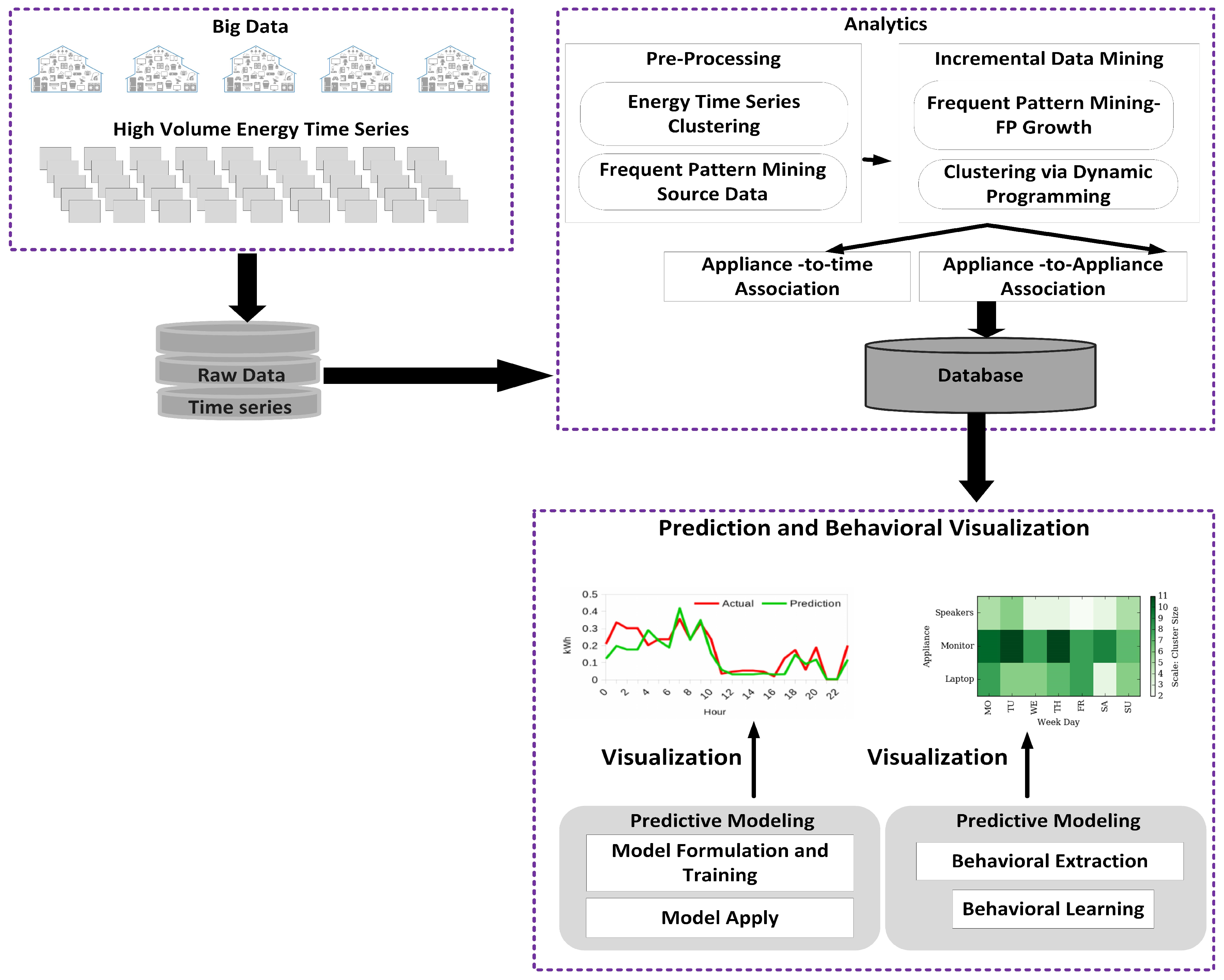
Figure 1 illustrates the proposed model with its distinct phases: pre-processing/data preparation, incremental frequent pattern mining and clustering analysis, association rules extraction, prediction and visualization. In this section, we discuss these phases and provide details about their respective mechanisms along with related theoretical background.
In the first phase, raw data, which contain millions of records of energy time series of consumption data, are prepared and processed for further analysis. In the following phase, incremental frequent pattern mining and clustering is performed. Frequent patterns are repeated itemsets or patterns that often appear in a dataset. Considering energy time series data, an itemset could comprise, for example, of a kettle and laptop and when this itemset is repeatedly encountered it is considered a frequent pattern. The aim is to uncover association and correlation between appliances in conjunction with understanding the time of appliance usage with respect to hours and time (Morning, Afternoon, Evening, Night) of day, weekdays, weeks, months and seasons. This latent information in energy time series data facilitates the discovery of appliance-time associations through clustering analysis of appliances over time. Clustering analysis is the process of constructing classes, where members of a cluster display similarity with one another and dissimilarity with members of other clusters. While learning these associations, it is important to identify what we refer to as Appliance of Interest (AoI), that is, major contributors to energy consumption, and develop capabilities to predict multiple appliance usages in time.
The mining of frequent patterns and cluster analysis are typically recognized as an off-line and expensive process on large size databases. However, in real-world applications, data generation is a continuous process, where new records are generated and existing ones may become obsolete as the time progresses, thereby, refuting existing frequent patterns and clusters and/or forming new associations and groups. This is the case of time series of energy consumption data, which is continuously generated at high resolution. Therefore, a progressive and incremental update approach is vital, where ongoing data updates are taken into account and existing frequent patterns and clusters are accordingly maintained with updated information. For example, an appliance such as a room-heater generally will be used during winter, and we can expect reduced usage frequency during other seasons. As an effect, a significant gain in use during winter but the decline in other seasons will be recorded. As a result, room-heater should appear higher on the list of frequent patterns and association rules during winter, but much lower during summer or spring. Similarly, appliance usage frequency would affect size or strength of clusters; i.e., association with time. This objective of capturing the variations can be achieved through progressive incremental data mining while eliminating the need to re-mine the entire database at regular intervals. For a large database, frequent pattern mining can be accomplished through pattern growth approach [38,39], whereas cluster analysis can be achieved through k-means clustering analysis [40]. In the proposed model, we expand these two techniques and present an online progressive incremental mining strategy where available data is recursively mined in quanta/slices of 24 h. This way, our data mining strategy can be viewed as an incremental process being administered every day. During each consecutive mining operation, existing frequent patterns and clusters are updated with new information, whereas new discovered patterns and clusters are appended to the persistent database in an incremental and progressive manner. With this technique, we mine only a fraction of the entire database at every iteration thus minimize memory overhead and accomplishing improved efficiency for real-world online applications where data generation is an ongoing process, and extraction of meaningful, relevant information to support continuous decision making at various levels is of paramount importance.
Frequent patterns and clusters can be stored and maintained in-memory using hash table data-structure or stored in off the memory Database Management System. The latter approach reduces memory requirement at the cost of a marginal increase in processing time, whereas the former approach reduces processing time but requires more memory. Considering the smart meter environment, quicker processing time is of importance; however, the persistence of information discovered through days, months or years is more vital to achieving useful and usable results for the future. Therefore, we prefer permanent storage using Database Management System over in-memory volatile storage.
In the third phase, the model extracts critical information of the appliance-appliance association rules from the appliance-appliance frequent patterns, incrementally and progressively. Frequent patterns discovered and clusters formed can determine the probabilistic association of appliance with other appliances and time while identifying AoIs. In the last phase, we use the Bayesian network based prediction approach, while taking in results from the previous phase, to predict the multiple appliance usages and energy consumption for both short-term and long-term forecasting. This phase includes the visualization of behavioral analytics and forecasting results.
The details of the mechanisms used in each phase are described in the following subsections.
2.1. Data Preparation
Energy time-series raw data is a high time-resolution data; it is transformed into a 1-min resolution energy consumption or load data. Afterwards, it is translated into a 30-min time-resolution source data for next stage of data mining process. Therefore, reducing data points to a readings per day per appliance, while recording usage duration, average load, and energy consumption for each active appliance. All the appliances registered active during this 30-min time interval are included in the source data for frequent pattern mining and cluster analysis. We analyzed and found time-resolution of 30-min as most suitable because it does not only capture appliance-time and appliance-appliance associations adequately but also keeps the number of patterns eligible for analysis sufficiently low and makes it appropriate for a real-world application. Three datasets (two real and one synthetic) were utilized for this research. The first real dataset has over 400 million raw energy consumption records from five houses having a time resolution of 6 s. It was reduced to just over 20 million during pre-processing phase without loss of accuracy or precision. Similarly, the second real dataset AMPds2 [34] was reduced to 4 million records from over 21 million raw records, which initially had 1-min time-resolution. Additionally, we constructed a synthetic dataset for preliminary evaluation of our model, having over 1.2 million records. In Table 1, Table 2 and Table 3, presents an example of source data comprising of four appliances for one house that is ready to mine for extraction of frequent patterns and clusters.
2.2. Frequent Pattern Mining and Association Rules Generation
Appliance-appliance and appliance-time associations represent critical consumer energy consumption behavioral characteristics and can identify peak load/energy consumption hours. These associations also explain respective behavioral traits and the expected comfort of the occupants. Therefore, with the gigantic volume of data continuously being gathered from smart meters, it is not only of avid interest to utilities and energy producers, but also to consumers to mine such frequent patterns and clusters for decision-making processes such as energy cost reduction, demand response optimization, and energy saving plans.
Frequent pattern mining which is conducted over the input data and presented in Table 1, can discover a recurring pattern; i.e., a pattern comprising of itemsets which exist repeatedly. In our case, these itemsets are individual appliances operating in specific houses/premises. Hence, the appliances appearing frequently together form frequent patterns are deemed to be associated. Therefore, the discovery of these frequent patterns aids us to identify appliance-appliance associations. The following subsection presents an introductory background on frequent pattern mining that is built on [41].
Let be an itemset consisting k items (appliances), which can be designated as k-itemset (). Let , denote a transaction database where every transaction is such that and . Table 1 represents sample of transaction database. Support count of the itemset can be defined as the frequency of its appearance; i.e., count of transactions that contain the itemset. Let, X () and Y () be set two itemsets or patterns. X and Y are considered frequent itemsets/patterns if their respective and are greater than or equal to . is a pre-determined minimum support count threshold. can be viewed as the probability of the itemset or pattern in the transaction database . It is also referred to as the relative support. Whereas, the frequency of occurrence is known as the absolute support. Hence, if the relative support of an itemset fulfills a pre-defined minimum support threshold , then the absolute support of X (or Y) satisfies the corresponding minimum support count threshold.
In the second stage of the (FP) mining process extracted frequent items, or frequent patterns are processed to develop association rules. Association rules, having configuration , are developed through employing – framework, where [Equation (1)] is the percentage of transactions having in the database that can be viewed as the probability . Additionally, the , as shown in equation [Equation (2)], can be described as the percentage of transactions, in transaction database , consisting of X that also contain Y; i.e., the conditional probability [41]. Equations (1) and (2) defines the notion of and respectively:
– frame-work is a common workhorse for the algorithms to extract frequent patterns and generate association rules. They eliminate uninteresting rules through comparing with and with . However, – frame-work do not examine correlation of the rule’s and . This makes this approach ineffective for eliminating uninteresting (association) rules. Therefore, it is vital to determine the correlation among the rules’ components to learn the negative or positive effect of their presence or absence and eliminate the rules that are deemed uninteresting. is one of the most generally employed correlation measures, but it has a negative impact of null-transactions. Null-transactions, are transactions where the possible constituents of association rules (itemsets) are not part of these transactions; i.e., null-transaction and null-transaction. In a large transaction database, null-transactions can outweigh the count for these itemsets. Thus, in a situation where minimum support threshold is low or extended patterns are of importance, the technique of using as criterion fails to yield results as described by [41]. The study proposes to use Kulczynski measure () in conjunction with the Imbalance Ratio () that are interestingness measures of null-invariant nature to supplement – frame-work in order to improve the efficiency of extracting rules that are interesting [41].
A correlation rule can be defined as:
Kulczynski Measure (Kulc) [41]: Kulczynski measure of X and Y, is an average of their . Considering the definition of this can be interpreted as the average of conditional probabilities for X and Y. or Kulczynski measure is null-invariant, and it is described as:
where,
- indicates that X and Y are negatively correlated; i.e., the occurrence of one indicates the absence of other
- , signifies that X and Y have positively correlation; i.e., occurrence one indicates presence of other
- signifies that X and Y are unrelated or independent having no correlation among them
Imbalance Ratio (IR) [41]: is used to asses the imbalance between and for a rule. It can be defined as:
where represent perfectly balanced and represent a very skewed context respectively. IR is null-invariant, and it is not affected by database size.
2.2.1. Extracting Frequent Pattern
In the work [38,39], the authors present FP-growth a pattern growth approach that utilizes divide-and-conquer depth-first technique. It starts by generating a frequent pattern tree or FP-tree, which is a compact form representation of the database transactions. An FP-tree stores the association information that is extracted from transactions with the support count for each component item. Next, for each frequent pattern item is derived from FP-Tree to mine or generate frequent patterns where the item that is under consideration is present. By employing this approach, only a divided portion that is relevant to the item and its corresponding growing patterns are examined that addresses both the deficiencies of the Apriori [42] technique. Moreover, we do not use minimum support threshold at the data mining phase to eliminate candidate patterns; rather we let the discovery of all the feasible frequent patterns. This change in approach ensures avoiding missing of any candidate pattern that may become a frequent pattern if the time slice is increased or mining activity is taken up for the complete database as a single process. All the frequent patterns extracted or discovered are stored in a persistent Database Management System, which ensures the continued availability of all the historical results to the consecutive mining operations. This is inline as discussed earlier. Additionally, new frequent patterns are compared with the frequent patterns in the database, and the for the patterns are updated if found to exists else the new pattern is added and stored in the persistent database. At the completion of each data mining activity, the is updated for all the frequent patterns in the database to make sure is computed all the time correctly. Algorithm 1 presents the incremental progressive frequent pattern mining technique, and corresponding results are shown in Table 4. Further, if we consider the definition of for an itemset in a database, which is the probability of the existence of the itemset in the transaction database, the marginal distribution for appliance-to-appliance association can be calculated at a global level. It is shown in Table 4. The computed marginal distribution establishes the probability of appliance being concurrently active.
| Algorithm 1 Frequent Pattern mining: Incremental. |
| Require: Transactional database (), Frequent patterns discovered storage database () Ensure: Incremental mining of frequent patterns, permanently stored in frequent patterns discovered storage database ()
|
2.2.2. Generating Association/Correlation Rules
Generation of appliance association rules is an uncomplicated process of extracting these rules from the frequent patterns for itemsets captured from transactions in a transaction database . We extract the association rules by extending the Apriori [42] technique. We propose to use the correlation measure to eliminate uninteresting association/correlation rules while use measure imbalance ratio to explain it.
2.3. Cluster Analysis: Incremental k-Means Clustering to Uncover Appliance-Time Associations
In addition to uncovering inter-appliance association, understanding the appliance-time association can aid critical analysis of consumer energy consumption behavior. Appliance-time associations can be defined in terms of hour of day (00:00–23:59), time of day (Morning/Afternoon/Evening/Night), weekday, week of month, week of year, month and/or season (Winter/Summer/Spring/Fall). Finding appliance-to-time associations can be seen as assembling of adequately adjoining time-stamps, for an active appliance that is recorded as operational, to construct a class or cluster for the given appliance. The clusters formed defines the appliance-to-time associations, while the size of clusters, determined by the count of members in the clusters, defines the relative strength of the clusters. Therefore, the finding of appliance-to-time associations can be interpreted as clustering of appliances into groups of time-intervals; where every cluster belongs to one appliance with time-stamps (data points) of activity as members of the cluster.
Cluster analysis is a process of constructing batches of data points according to the information retrieved from the data, but without external intervention; i.e., unsupervised classification. This extracted information outlines the relationship among the data points and acts as the base for classification to ensure data points within a cluster are closer to one another but distant from members of other clusters [43,44]. “Closer” and “Distant” are measures of association, defining how closely members of a cluster are related to one another. Hence, clustering analysis conducted over the input data, presented in Table 2 and Table 3, can generate clusters or classes defining natural associations of appliances with time while respective support or strength defines the degree of association. These appliance-to-time associations are capable of not only determining peak load or energy consumption hours but can reveal the energy consumption behavioral characteristics of occupants or consumers as well.
We extend one of the most widely used prototype-based partitional clustering technique to extract appliance-time associations. The prototype of a cluster is defined by its centroid, which is the mean of all the member data points. In this approach, clusters are formed from non-overlapping distinct groups; i.e., each member data point belongs to one and only one group or cluster [43]. Moreover, we mine data incrementally in a progressive manner, which we explain next.
2.3.1. k-Means Cluster Analysis
We introduce preliminary background on k-means clustering based on [43,44]. For a dataset, , that has n data points in the Euclidean space, partitional clustering allocates the data points from dataset into k number of clusters, , having centroids such that , and for (). An objective function that is based on Euclidean distance, Equation (7), is employed to measure the cohesion between data points that demonstrate the quality of the cluster. The objective function is defined as the sum of the squared error (SSE), define in Equation (6), and k-means clustering algorithm strives to minimize the SSE.
The k-means starts by selecting k data points from , where , and form k clusters having centroids or cluster centers as the selected data points. Next, for each of the remaining data points d in , data point is assigned to a cluster having least Euclidean distance from its centroid () i.e., . After a new data point is assigned the revised cluster centroids are determined by computing the cluster centers for the clusters, and k-means algorithm repetitively refines the cluster composition to reduce intra-cluster dissimilarities by reassigning the data points until clusters are balanced; i.e., no reassignment is possible, while evaluating the cluster quality by computing the sum of the squared error (SSE) covering all the data points in the cluster from its centroid.
2.3.2. Optimal k: Determining k using
We exploit that is calculated based on the Euclidean distance, to ascertain the optimal number of clusters; i.e., k, while assessing the quality of clustering by analyzing intra-cluster cohesion and inter-cluster separation of data points among clusters. measures the degree of similarities and dissimilarities to indicates “How well clusters are formed?”. can be computed as defined in Equations (8)–(12) [45],
- Compute as average distance of to all other data points in cluster
- Compute Average distance of to all other data points in clusters , having ; Determine = across all the clusters except .
- Compute for
- Compute for cluster
- Compute for clustering, having k clusters
can range from −1 to 1; where a negative value indicates misfit as the average distance of data point to data points in the cluster () is greater than the average distance to data points in a cluster other than () , and a positive number indicates better-fit clusters. Overall the quality of the cluster can be assessed by computing average by computing the average of () for all the member data points for the cluster, as shown in Equation (11). Similarly, an average () can be calculated for complete clustering by obtaining the average of for all the member data points across all the clusters, as in Equation (12) [45].
Finally, to determine optimal , where n is the unique set of data points in database/dataset, the process of analyzing the quality of clusters formed is repeated while computing () and k is chosen having maximum .
2.3.3. Optimal One-Dimensional k-Means Cluster Analysis: Dynamic Programming
With reference to the clustering input database, presented in Table 2 and Table 3, we have a cluster analysis requirement for a single dimension data. We make use of dynamic programming algorithm for optimal one-dimensional k-means clustering proposed by [46], which ensures optimality and efficient runtime. We further extend the algorithm to achieve incremental data mining to discover appliance-time associations.
Here we provide the relevant background based on [46]. A one-dimension k-means cluster analysis can be viewed as grouping n data points into k clusters, while minimizing sum of the squared error (SSE), shown in Equation (6). A sub-problem for the original dynamic programming problem can be defined as finding the minimum SSE of clustering data points into m clusters. The respective minimum SSE are stored in a Distance Matrix () of size , where records the minimum SSE for the stated sub-problem, and provides the minimum SSE for the original problem. For a data point in the m clusters, where is the first data element of cluster m, the optimal solution (SSE) to the sub-problem is ; therefore, must be the optimal SSE for the first data points in the clusters. This provides optimal substructure defined by Equation (13).
where is the computed SSE for from their centroid/cluster center, and , for or . is computed iteratively from as shown in Equation (14) .
where, is the mean of the first data elements.
A backtrack matrix is maintained, of size , to record the starting index of the first data element of respective cluster. Backtrack matrix is used to extract cluster members by determining the starting and ending indices for the corresponding cluster and retrieving the data points from the original dataset. Equation (16) captures this notion.
2.3.4. Incremental Mining: Cluster Analysis
We achieve incremental progressive clustering by merging clusters and/or adding new clusters extracted during each successive mining operation into a persistent database in the Database Management System. Discovered clusters database records all the relevant cluster parameters and information that includes centroid, (width), SSE, and data points along with their distance from the centroid. This enables the easy addition of new data points or clusters while computing cluster parameters with respect to the newly added data points and updating the information in the database accordingly. Considering, the translation of the raw time series data into a source data having 30 min time-resolution during the data preparation phase, this time-resolution unit is sufficient to capture vital information regarding consumer energy consumption decision patterns. The cluster analysis for hour of day done on this source data will result in clusters created with a separation between clusters’ centroids as multiples of such time-resolution, which is 30 min in the current case. This time-resolution is identified as . Whereas, a cluster analysis on the other bases such as time of day, weekday, week of month, week of year, month and seasons have natural segmentation. With this operation, we achieve more exclusive homogeneity and separation among clusters.
Upon completion of mining on the incremental quantum of data, newly discovered clusters are matched against the existing clusters in the database to determine the closest cluster(s) to merge with, having centroid within the distance of from the new cluster. If there exists no cluster in the database, which is closer to the new cluster satisfying the permissible centroid distance constraint, the new cluster is added/stored into the discovered clusters database with all the accompanying parameters and information. However, in the case of success, data points from the new cluster will be added to the searched cluster(s) while evaluating the quality of the final cluster by computing the . The data points from the new cluster are picked according to increasing order of distance from the centroid. The most stable cluster configuration, having the maximum , are saved to the database. Algorithm 2 outlines the incremental cluster analysis using one-dimensional k-means clustering via dynamic programming and results are presented in Table 5. During the analysis of the clustering results, it can be noted that for a cluster centroid, the marginal distribution for the appliances at a global level can be computed as shown in Table 6. The computed marginal distribution decides the probability of appliances being operational or active during the period identified by the centroid.
| Algorithm 2 Incremental k-means Clustering. |
| Require: Transactional database , permissible centroid distance between clusters = 30 Ensure: Incremental k-means clustering, clusters and associated configuration (, SSE, and data points along with distance from centroid) stored in clusters discovered database
|
2.4. Bayesian Network for Multiple Appliance Usage Prediction and Household Energy Forecast
We utilize a Bayesian Network (BN) that is a probabilistic graphical model using directed acyclic graph (DAG) to predict the multiple appliances usage at some point in the future. Bayesian networks are directed acyclic graphs, where nodes symbolize random variables and edges represent probabilistic dependencies among them. Each node or variable in BN is autonomous; i.e., it does not depend on its nondescendants. It is accompanied by local conditional probability distribution in the form of a node probability table that aids the determination of the joint conditional probability distribution for the complete model [47,48]. Therefore, the local probability distributions furnish quantitative probabilities that can be multiplied according to qualitative independencies described by the structure of Bayesian Network to obtains the joint probability distributions for the model. The Bayesian network has advantages such as the ability to effectively make use of historical facts and observations, learn relationships, mitigate missing data while preventing overfitting of data [49]. A Bayesian network can be illustrated by the probabilistic distribution defined by Equation (17) [50,51].
2.4.1. Probabilistic Prediction Model
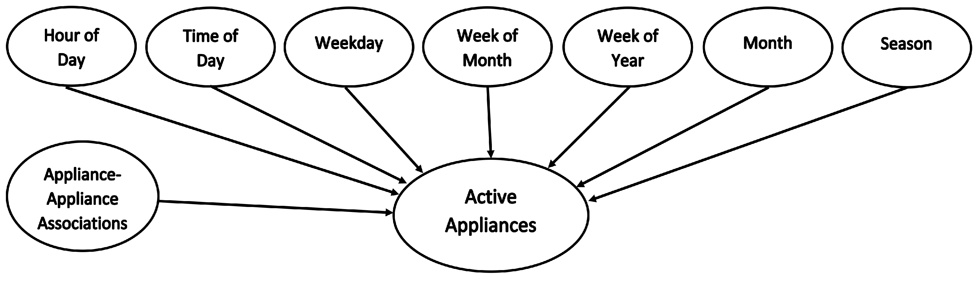
We construct our model based on Bayesian network, having eight nodes representing probabilities for appliances-to-time associations in terms of hour of day (00:00–23:59), time of day (Morning/Afternoon/Evening/Night), weekday, week of month, week of year, month and/or season (Winter/Summer/Spring/Fall), and appliance-appliance associations. The resulting Bayesian network has a very simple topology, with known structure and full observability, comprising only one level of input evidence nodes, accompanied by respective unconditional probabilities, converging to one output node. The Equation (18) and Figure 2 present the posterior probability or marginal distribution and network structure for the proposed prediction model.
We use the output of the earlier two phases; i.e., cluster analysis and frequent pattern mining to train the model, which effectively incrementally learns the prior information through progressive mining. Table 7 represents a sample of the training data with marginal distribution for the various appliances, and the probability of appliances to be active during the period, for the node variable/parameter vector. The probabilities are computed from the clusters, formed and contentiously updated during the mining operation. The respective cluster strength or size determines the relative probability for the individual appliance. Additionally, appliance-appliance association, the outcome of the frequent pattern mining, computes the probabilities for the appliances to operate or be active concurrently. Therefore, the model uses top-down reasoning to deduce and predict active appliances consuming energy, operating concurrently, using historical evidence from the results of cluster analysis (appliance-to-time associations) and frequent pattern mining (appliance-to-appliance associations).
Furthermore, the multiple appliance usage prediction results build the foundation for household energy consumption forecast, where, average appliance load and average appliance usage duration are extracted from the historical raw time-series data at the respective time resolution that is an hour, weekday, week, month or season level. In this way, we are capable of predicting energy consumption for a defined time in the future for short-term: from the next hour up to 24 h and long-term: days, weeks, months, or seasons. Next, we evaluate our proposed model and provide results of the analysis. Table 8 shows an example of extracted raw data for data mining for one appliance.
3. Evaluation and Results
We performed thorough data mining experimentation using time-series energy consumption data from two datasets UK-Dale [33] and AMPds2 [34] in addition to a synthetic dataset prepared for training purposes. The evaluation results clearly support our hypothesis regarding the impact of human behavior on energy consumption patterns. This is reflected in the analysis of appliance-to-appliance and appliance-to-time usage correlations. Although it is important to note that our proposed approach can be applied to any quantum size for incremental mining, we considered 24 h as the most optimal selection of time-span to retrieve underlying essential information. We obtained consistent results during evaluation for all the houses in the datasets; but, due to space constraint we present appliance-appliance, and appliance-time associations result from one house and prediction statistics for all the houses.
Moreover, we make use of a multi-label SVM classifier, based on Binary Relevance (a One-vs.-All (OvA) approach) algorithm as a problem transformation method [52] and Multi-layer Perceptron (MLP) multi-label classifier algorithm that trains using Backpropagation to predict the operation of multiple appliances to compare the results and accuracy of the proposed model. Our choice of models for comparison is based on the wide use of these classification techniques, SVM and MLP, and wide acceptance as two well-known approaches for classification and prediction by the research community [53,54,55,56,57,58,59,60,61,62,63,64].
Further, we are considering a context-aware time series data from smart meter; i.e., energy consumption measurements are tagged with appliance details. In the current scope of work, we have taken into account two key features or variables; i.e., a time-stamp (at the hour, minute, day, weekday, week, month, and season) and energy consumption measurement at appliance level. This provides us data with reduced dimensions for data mining. All the approaches; i.e., proposed model and models chosen for comparative study (SVM, and MLP) use these features.
3.1. Results Analysis and Discussion
Table 9 presents the extracted appliance-appliance associations outcome of processing 25% of the data from the respective dataset for House 3. We noticed that appliances such as Laptop, Monitor, and Speakers manifest associations; and during further steps of the incremental mining, associations among these appliances strengthen and new appliances such as Washing Machine, Kettle, and Running Machine develop associations. From these associations, we can infer the occupants’ behavioral preferences such as “occupants like to work on the computer and/or listen to music while washing clothes” and “work on the computer and/or workout while cooking”.
Furthermore, Table 10 presents the appliance usage priorities, which are revealed from the habitual use of certain appliances. This led us to determine what we refer to as Appliance-of-Interest (AoI), which are the appliances having a low power rating, but they have large energy footprints due to excessive use. This is clear for appliances Speakers, Laptop, and Monitor in House 3. They are identified as appliances that are habitually used over extended periods; therefore, they are major contributors to electricity usage. This conclusion is often neglected by consumers when they try to identify the higher cost of electricity. In other words, large appliances that often have higher power ratings are not always the source of higher cost of electricity; it is often small appliances that are used excessively due to consumers’ behavior are responsible for it. Moreover, we found that other appliances such as Kettle, Toaster, and Microwave; i.e., appliances with higher power rating contribute towards peak power (kW) load but overall energy (kWh) consumption is higher for appliances identified as AoI.
The carried extensive analysis of energy consumption for the peak load and peak energy revealed homogeneous trends across the board.
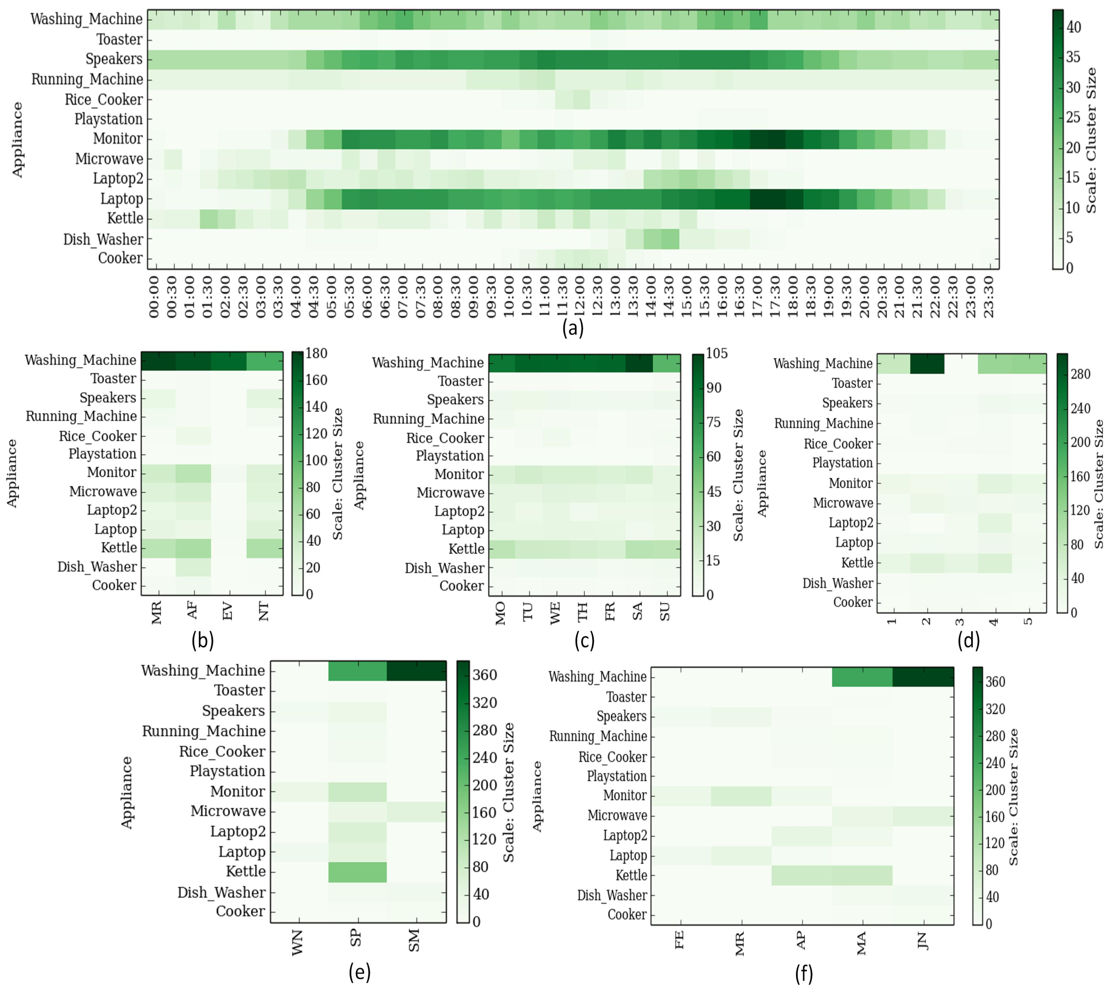
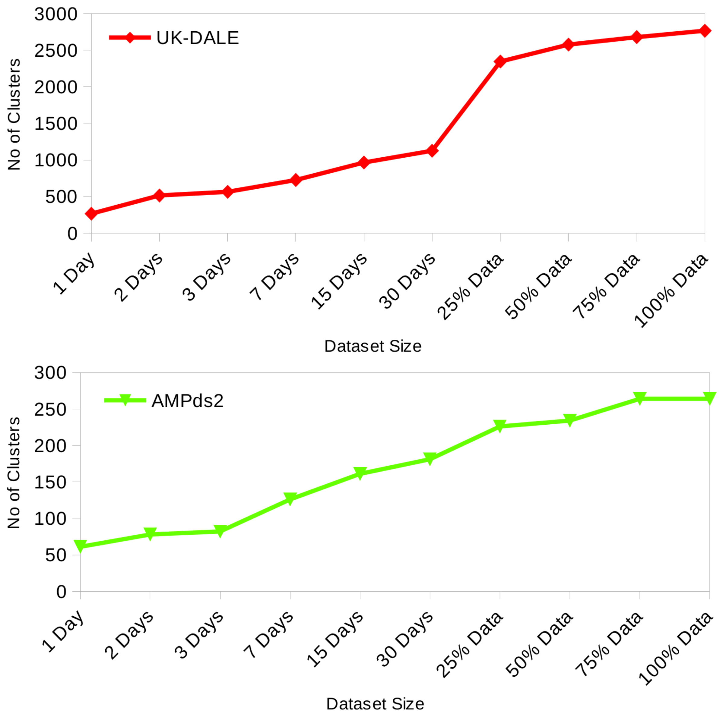
Next, Figure 3 shows the appliance-time associations discovered. We can see that Laptop and Monitor are two appliances which are used simultaneously and with the highest concentration of use during 17:00–18:00 with similar frequency of use during the week but increased usage in spring. Whereas, Washing Machine is used all day long with major usage concentration noted between 05:45–07:15 and 15:15–17:15 with increased usage on Saturdays and during the summer season. Based on the above-mentioned behavior, we realized the changing impact of time, days and seasons on appliance usages. Figure 4 outlines the number of clusters formed during the incremental data mining process; which further confirms the discovery of new appliance-time associations representative of behavioral changes taking place over a period of time.
We utilized the above appliance-appliance and appliance-time associations, in our probabilistic prediction model to forecast multiple co-occurrence usages of appliances with high success. Table 11 shows the forecasting accuracy attained for short and long-term as well as the overall predictions when performing incremental data mining processes using 25%, 50% and 75% of the dataset. Our proposed model outperformed SVM and MLP at each stage while attaining an overall accuracy of 81.82% (25%), 85.90% (50%), 89.58% (75%) at each mining process, respectively. Figure 5 presents the comparison of the accuracy proposed model vs. SVM and MLP while supporting our hypothesis that incremental mining can discover variations induced by dissimilarities of occupants’ behavioral traits and facilitate well-informed energy consumption decision-making at various levels. Additionally, Table 12 presents and compares the accuracy of the model at the household level.
Subsequently, we applied our results of multiple appliance predictions to forecast the expected household energy consumption. We achieved accuracies of 81.89%, 75.88%, 79.23%, 74.74%, and 72.81% for short-term @ hour, long-term @ day, long-term @ week, long-term @ month, and long-term @ season energy consumption predictions respectively. Figure 6 presents and compares the energy prediction against actual energy consumption for House 3.
Considering the above results, we note the robust evidence of the influence of consumer behavior on household energy consumption patterns, which can be learned through appliance-to-appliance and appliance-to-time associations derived from the frequent pattern mining and cluster analysis. We observed through incremental association discovery that the associations change over time, and are directly affected by occupants’ behavior. Also, the choice of use of appliances, whether increased or reduced usage frequency, depends on the time (time of day, days, week, season, etc.); for example, from Figure 3, we observed that the kettle in house 3 was used more around 01:30 a.m. on Mondays, Saturdays, and Sundays on the second and the fourth weeks of the months, and during Spring but less otherwise. These choices made by occupants affect the energy consumption decision patterns that get directly translated into energy usage. Therefore, energy consumption behavior for different occupants is affected by these parameters differently depending on their lifestyle. In other words, the occupants’ behavior has a direct influence on household energy consumption. Acknowledging and learning these variations, which are the result of the occupants’ behavioral traits and corresponding personal preferences, are crucial for designing successful energy reduction programs that encourage consumers to participate.
3.2. Dataset and System Setup
The model evaluation and experiments were run on two energy time series datasets collected from real houses. The first one is the UK Domestic Appliance Level Electricity dataset (UK-Dale) [33], which includes 4 years worth of energy time series data collected from five houses in Southern England between 2012 and 2015. Furthermore, this energy time series dataset entails a total of 109 appliances with time resolution of 6 s. This dataset is published by UK Energy Research Centre Energy Data Centre (UKERC-EDC) and considered one of the largest energy time series with approximately half a billion records [33]. The second energy time series dataset is AMPds2-Almanac of Minutely Power dataset [34], which is a time series data for electricity, water, and natural gas measurements for over 2 years from 2012 to 2014, with a time resolution of 1 minute for one residential house from Greater Vancouver metropolitan area in British Columbia, Canada. This dataset includes weather data from Environment Canada. Electrical measurements are done at the electrical circuit breaker panel using DENT PowerScout 18 Multi-Circuit Power Submeters. For model training and initial experiments, we prepared a new synthetic dataset using seeds from real dataset [65] by ISSDA-The Irish Social Science Data Archive. The synthetic dataset contains over 1.2 million records of energy time series at 1 min time resolution from one house containing data about 21 appliances. Table 8 shows an example of extracted raw data for data mining for one appliance. The entire system was developed using Python, where data is stored in MySQL and MongoDB databases on a ubuntu 14.04 LTS 64-bit system.
4. Conclusions and Future Work
This work demonstrates the impact of consumers’ behavior and personal preferences on energy consumption decision patterns, which can be inferred from appliance-appliance and appliance-time associations learned from energy time series. These patterns can facilitate sustainable energy saving plans for consumers, balance energy supply, and demand through optimizing scheduling and allocation, plan energy purchasing policies and maintenance routines and on a broader scale balance the smart grid’s production and strategic planning.
Furthermore, this paper presented unsupervised incremental frequent mining and forecasting model utilizing the Bayesian network and dynamic programming principles. Exhaustive experiments using various time periods such as 15 min, 30 min, 1 h, 2 h, 6 h, and 12 h have revealed fairly comparable results that supported our incremental mining approach. Therefore, we introduced a new parameter to select the time quanta, which can be chosen during data transformation step to define the smallest possible mining time period. The model transforms data in such a fashion that a dynamic switch in time quantum can be accommodated without having to restart the process. By altering the time quantum, it is possible to reduce the number of appliances and data size under consideration for data mining.
Furthermore, the proposed model is evaluated using real-world context-rich energy time series datasets. We showed that our system outperforms Support Vector Machine (SVM) and Multi-layer Perceptron (MLP). For future work, we are planning to conduct further refinement on the proposed model and introduce real-time distributed learning of big data mining of energy time series from multiple houses. This will allow utilities to perform online/real-time energy predictions to momentarily engage consumers upon realizing consumption changes for an improved smart grid energy saving programs.
Author Contributions
All authors contributed to this work by collaboration.
Conflicts of Interest
The authors declare no conflict of interest. The founding sponsors had no role in the design of the study; in the collection, analyses, or interpretation of data; in the writing of the manuscript, and in the decision to publish the results.
Abbreviations
The following abbreviations are used in this manuscript:
| AMPds2 | The Almanac of Minutely Power dataset (Version 2) |
| AoI | Appliances of Interest |
| BN | Bayesian Network |
| FP | Frequest Pattern |
| IR | Imbalance Ratio |
| Kulc | Kulczynski measure |
| MLP | Multi-Layer Perceptron |
| SVM | Support Vector Machine |
| UK-Dale | UK Domestic Appliance Level Electricity dataset |
References
- Chen, Y.C.; Hung, H.C.; Chiang, B.Y.; Peng, S.Y.; Chen, P.J. Incrementally Mining Usage Correlations among Appliances in Smart Homes. In Proceedings of the 2015 18th International Conference on Network-Based Information Systems (NBiS), Taipei, Taiwan, 2–4 September 2015; pp. 273–279. [Google Scholar]
- Anca-Diana, B.; Nigel, G.; Gareth, M. Achieving Energy Efficiency Through Behaviour Change: What Does It Take? Technical Report; European Economic Area (EEA): Geneva, Switzerland, 2013. [Google Scholar]
- Zipperer, A.; Aloise-Young, P.A.; Suryanarayanan, S.; Roche, R.; Earle, L.; Christensen, D.; Bauleo, P.; Zimmerle, D. Electric Energy Management in the Smart Home: Perspectives on Enabling Technologies and Consumer Behavior. Proc. IEEE 2013, 101, 2397–2408. [Google Scholar] [CrossRef]
- Wood, G.; Newborough, M. Dynamic energy-consumption indicators for domestic appliances: Environment, behaviour and design. Energy Build. 2003, 35, 821–841. [Google Scholar] [CrossRef]
- Wood, G.; Newborough, M. Influencing user behaviour with energy information display systems for intelligent homes. Int. J. Energy Res. 2007, 31, 56–78. [Google Scholar] [CrossRef]
- Hawarah, L.; Ploix, S.; Han Jacomino, M. User Behavior Prediction in Energy Consumption in Housing Using Bayesian Networks; Chapter User Behavior Prediction in Energy Consumption in Housing Using Bayesian Networks. In Proceedings of the 10th International Conference on Artificial Intelligence and Soft Computing, ICAISC 2010, Zakopane, Poland, 13–17 June 2010; Springer: Berlin/Heidelberg, Germany, 2010; Volume 6113, pp. 372–379. [Google Scholar]
- Basu, K.; Debusschere, V.; Bacha, S. Appliance usage prediction using a time series based classification approach. In Proceedings of the IECON 2012-38th Annual Conference on IEEE Industrial Electronics Society, Montreal, QC, Canada, 25–28 October 2012; pp. 1217–1222. [Google Scholar]
- Basu, K.; Hawarah, L.; Arghira, N.; Joumaa, H.; Ploix, S. A prediction system for home appliance usage. Energy Build. 2013, 67, 668–679. [Google Scholar] [CrossRef]
- Rollins, S.; Banerjee, N. Using rule mining to understand appliance energy consumption patterns. In Proceedings of the 2014 IEEE International Conference on Pervasive Computing and Communications (PerCom), Budapest, Hungary, 24–28 March 2014; pp. 29–37. [Google Scholar]
- Ong, L.; Bergés, M.; Noh, H.Y. Exploring Sequential and Association Rule Mining for Pattern-based Energy Demand Characterization. In Proceedings of the 5th ACM Workshop on Embedded Systems For Energy-Efficient Buildings, Roma, Italy, 11–15 November 2013; ACM: New York, NY, USA, 2013; pp. 25:1–25:2. [Google Scholar]
- Chelmis, C.; Kolte, J.; Prasanna, V.K. Big data analytics for demand response: Clustering over space and time. In Proceedings of the 2015 IEEE International Conference on Big Data (Big Data), Santa Clara, CA, USA, 29 October–1 November 2015; pp. 2223–2232. [Google Scholar]
- Quilumba, F.L.; Lee, W.J.; Huang, H.; Wang, D.Y.; Szabados, R.L. Using Smart Meter Data to Improve the Accuracy of Intraday Load Forecasting Considering Customer Behavior Similarities. IEEE Trans. Smart Grid 2015, 6, 911–918. [Google Scholar] [CrossRef]
- Viegas, J.L.; Vieira, S.M.; Sousa, J.M.C.; Melicio, R.; Mendes, V.M.F. Electricity demand profile prediction based on household characteristics. In Proceedings of the 2015 12th International Conference on the European Energy Market (EEM), Lisbon, Portugal, 19–22 May 2015; pp. 1–5. [Google Scholar]
- Liao, Y.S.; Liao, H.Y.; Liu, D.R.; Fan, W.T.; Omar, H. Intelligent Power Resource Allocation by Context-Based Usage Mining. In Proceedings of the 2015 IIAI 4th International Congress on Advanced Applied Informatics (IIAI-AAI), Okayama, Japan, 12–16 July 2015; pp. 546–550. [Google Scholar]
- Gajowniczek, K.; Zabkowski, T. Data Mining Techniques for Detecting Household Characteristics Based on Smart Meter Data. Energies 2015, 8, 7407–7427. [Google Scholar] [CrossRef]
- Zhang, P.; Wu, X.; Wang, X.; Bi, S. Short-term load forecasting based on big data technologies. CSEE J. Power Energy Syst. 2015, 1, 59–67. [Google Scholar] [CrossRef]
- Schweizer, D.; Zehnder, M.; Wache, H.; Witschel, H.F.; Zanatta, D.; Rodriguez, M. Using Consumer Behavior Data to Reduce Energy Consumption in Smart Homes: Applying Machine Learning to Save Energy without Lowering Comfort of Inhabitants. In Proceedings of the 2015 IEEE 14th International Conference on Machine Learning and Applications (ICMLA), Miami, FL, USA, 9–11 December 2015; pp. 1123–1129. [Google Scholar]
- Hassani, M.; Beecks, C.; Tows, D.; Seidl, T. Mining Sequential Patterns of Event Streams in a Smart Home Application. In Proceedings of the LWA 2015 Workshops: KDML, FGWM, IR, and FGDB, Trier, Germany, 7–9 October 2015. [Google Scholar]
- Perez-Chacon, R.; Talavera-Llames, R.; Martinez-Alvarez, F.; Troncoso, A. Finding electric energy consumption patterns in big time series data. In Proceedings of the 13th International Conference Distributed Computing and Artificial Intelligence, Seville, Spain, 1–3 June 2016; pp. 231–238. [Google Scholar]
- Ardakanian, O.; Koochakzadeh, N.; Singh, R.P.; Golab, L.; Keshav, S. Computing Electricity Consumption Profilesfrom Household Smart Meter Data. In Proceedings of the Workshops of the EDBT/ICDT 2014 Joint Conference (EDBT/ICDT 2014), Athens, Greece, 28 March 2014; pp. 140–147. [Google Scholar]
- Kwac, J.; Flora, J.; Rajagopal, R. Household Energy Consumption Segmentation Using HoURLy Data. IEEE Trans. Smart Grid 2014, 5, 420–430. [Google Scholar] [CrossRef]
- Truong, N.C.; McInerney, J.; Tran-Thanh, L.; Costanza, E.; Ramchurn, S.D. Forecasting Multi-appliance Usage for Smart Home Energy Management. In Proceedings of the Twenty-Third International Joint Conference on Artificial Intelligence, Beijing, China, 3–9 August 2013; AAAI Press: Palo Alto, CA, USA, 2013; pp. 2908–2914. [Google Scholar]
- Kavousian, A.; Rajagopal, R.; Fischer, M. Determinants of residential electricity consumption: Using smart meter data to examine the effect of climate, building characteristics, appliance stock, and occupants’ behavior. Energy 2013, 55, 184–194. [Google Scholar] [CrossRef]
- Missaoui, R.; Joumaa, H.; Ploix, S.; Bacha, S. Managing energy Smart Homes according to energy prices: Analysis of a Building Energy Management System. Energy Build. 2014, 71, 155–167. [Google Scholar] [CrossRef]
- Virote, J.; Neves-Silva, R. Stochastic models for building energy prediction based on occupant behavior assessment. Energy Build. 2012, 53, 183–193. [Google Scholar] [CrossRef]
- Zhao, H.X.; Magoulès, F. A review on the prediction of building energy consumption. Renew. Sustain. Energy Rev. 2012, 16, 3586–3592. [Google Scholar] [CrossRef]
- Deb, C.; Zhang, F.; Yang, J.; Lee, S.E.; Shah, K.W. A review on time series forecasting techniques for building energy consumption. Renew. Sustain. Energy Rev. 2017, 74, 902–924. [Google Scholar] [CrossRef]
- Liu, D.; Chen, Q.; Mori, K. Time series forecasting method of building energy consumption using support vector regression. In Proceedings of the 2015 IEEE International Conference on Information and Automation, Lijiang, China, 8–10 August 2015. [Google Scholar]
- Zhang, F.; Deb, C.; Lee, S.E.; Yang, J.; Shah, K.W. Time series forecasting for building energy consumption using weighted Support Vector Regression with differential evolution optimization technique. Energy Build. 2016, 126, 94–103. [Google Scholar] [CrossRef]
- Biswas, M.R.; Robinson, M.D.; Fumo, N. Prediction of residential building energy consumption: A neural network approach. Energy 2016, 117, 84–92. [Google Scholar] [CrossRef]
- Torres, J.F.; Fernández, A.M.; Troncoso, A.; Martínez-Álvarez, F. Deep Learning-Based Approach for Time Series Forecasting with Application to Electricity Load. In Biomedical Applications Based on Natural and Artificial Computing; Springer: Cham, Switzerland, 2017; pp. 203–212. [Google Scholar]
- Li, C.; Ding, Z.; Zhao, D.; Yi, J.; Zhang, G. Building Energy Consumption Prediction: An Extreme Deep Learning Approach. Energies 2017, 10, 1525. [Google Scholar] [CrossRef]
- Jack, K.; William, K. The UK-DALE dataset, domestic appliance-level electricity demand and whole-house demand from five UK homes. Sci. Data 2015, 2. [Google Scholar] [CrossRef]
- Makonin, S.; Ellert, B.; Bajic, I.V.; Popowich, F. AMPds2-Almanac of Minutely Power dataset: Electricity, water, and natural gas consumption of a residential house in Canada from 2012 to 2014. Sci. Data 2016, 3. [Google Scholar] [CrossRef] [PubMed]
- Singh, S.; Yassine, A. Incremental Mining of Frequent Power Consumption Patterns from Smart Meters Big Data. In Proceedings of the IEEE Electrical Power and Energy Conference 2016-Smart Grid and Beyond: Future of the Integrated Power System, Ottawa, ON, Canada, 12–14 October 2016. [Google Scholar]
- Singh, S.; Yassine, A. Mining Energy Consumption Behavior Patterns for Households in Smart Grid. IEEE Trans. Emerg. Top. Comput. 2017, PP. [Google Scholar] [CrossRef]
- Yassine, A.; Singh, S.; Alamri, A. Mining Human Activity Patterns From Smart Home Big Data for Health Care Applications. IEEE Access 2017, 5, 13131–13141. [Google Scholar] [CrossRef]
- Han, J.; Pei, J.; Yin, Y. Mining Frequent Patterns Without Candidate Generation. In Proceedings of the 2000 ACM SIGMOD International Conference on Management of Data, Dallas, TX, USA, 15–18 May 2000; ACM: New York, NY, USA, 2000; pp. 1–12. [Google Scholar]
- Han, J.; Pei, J.; Yin, Y.; Mao, R. Mining Frequent Patterns without Candidate Generation: A Frequent-Pattern Tree Approach. Data Min. Knowl. Discovery 2004, 8, 53–87. [Google Scholar] [CrossRef]
- MacQueen, J. Some methods for classification and analysis of multivariate observations. In Proceedings of the Fifth Berkeley Symposium on Mathematical Statistics and Probability, Oakland, CA, USA, 21 June–18 July 1965; University of California Press: Berkeley, CA, USA, 1967; Volume 1, pp. 281–297. [Google Scholar]
- Han, J.; Pei, J.; Kamber, M. Mining Frequent Patterns, Associations, and Correlations: Basic Concepts and Methods. In Data Mining: Concepts and Techniques, 3rd ed.; Morgan Kaufmann: Burlington, MA, USA, 2011; Chapter 6; pp. 243–278. [Google Scholar]
- Agrawal, R.; Srikant, R. Fast Algorithms for Mining Association Rules in Large Databases. In Proceedings of the 20th International Conference on Very Large Data Bases, Santiago, Chile, 12–15 September 1994; Morgan Kaufmann Publishers Inc.: San Francisco, CA, USA, 1994; pp. 487–499. [Google Scholar]
- Tan, P.N.; Steinbach, M.; Kumar, V. Cluster Analysis: Basic Concepts and Algorithms. In Introduction to Data Mining; Pearson: London, UK, 2005; Volume 1, Chapter 8; pp. 487–568. [Google Scholar]
- Han, J.; Pei, J.; Kamber, M. Cluster Analysis: Basic Concepts and Methods. In Data Mining: Concepts and Techniques, 3rd ed.; Morgan Kaufmann: Burlington, MA, USA, 2011; Chapter 10; pp. 443–494. [Google Scholar]
- Rousseeuw, P.J. Silhouettes: A graphical aid to the interpretation and validation of cluster analysis. J. Comput. Appl. Math. 1987, 20, 53–65. [Google Scholar] [CrossRef]
- Haizhou, W.; Mingzhou, S. Ckmeans.1d.dp: Optimal k-means Clustering in One Dimension by Dynamic Programming. R J. 2011, 3, 29–33. [Google Scholar]
- Ben-Gal, I. Bayesian Networks. In Encyclopedia of Statistics in Quality and Reliability; John Wiley & Sons, Ltd.: Hoboken, NJ, USA, 2008. [Google Scholar]
- Pearl, J. Probabilistic Reasoning in Intelligent Systems: Networks of Plausible Inference; Morgan Kaufmann Publishers Inc.: San Francisco, CA, USA, 1988. [Google Scholar]
- Heckerman, D. Bayesian Networks for Data Mining. Data Min. Knowl. Discov. 1997, 1, 79–119. [Google Scholar] [CrossRef]
- Barber, D. Belief Networks. In Bayesian Reasoning and Machine Learning; Cambridge University Press: Cambridge, UK, 2012; Chapter 3; pp. 29–57. [Google Scholar]
- Han, J.; Pei, J.; Kamber, M. Classification: Advanced Methods. In Data Mining: Concepts and Techniques, 3rd ed.; Morgan Kaufmann: Burlington, MA, USA, 2011; Chapter 9; pp. 243–278. [Google Scholar]
- Tsoumakas, G.; Katakis, I.; Vlahavas, I. Mining Multi-label Data. In Data Mining and Knowledge Discovery Handbook; Springer: Boston, MA, USA, 2010; pp. 667–685. [Google Scholar]
- Niska, H.; Koponen, P.; Mutanen, A. Evolving smart meter data driven model for short-term forecasting of electric loads. In Proceedings of the 2015 IEEE Tenth International Conference on Intelligent Sensors, Sensor Networks and Information Processing (ISSNIP), Singapore, 7–9 April 2015. [Google Scholar]
- Depuru, S.S.S.R.; Wang, L.; Devabhaktuni, V. Support vector machine based data classification for detection of electricity theft. In Proceedings of the 2011 IEEE/PES Power Systems Conference and Exposition, Phoenix, AZ, USA, 20–23 March 2011. [Google Scholar]
- Gajowniczek, K.; Ząbkowski, T. Short Term Electricity Forecasting Using Individual Smart Meter Data. Procedia Comput. Sci. 2014, 35, 589–597. [Google Scholar] [CrossRef]
- Lee, J.S.; Tong, J.D. Applications of support vector machines to standby power reduction. In Proceedings of the 2016 IEEE International Conference on Systems, Man, and Cybernetics (SMC), Budapest, Hungary, 9–12 October 2016; pp. 002738–002743. [Google Scholar]
- Zhang, Y.; Wang, L.; Sun, W.; Green, R.C., II; Alam, M. Distributed Intrusion Detection System in a Multi-Layer Network Architecture of Smart Grids. IEEE Trans. Smart Grid 2011, 2, 796–808. [Google Scholar] [CrossRef]
- Nagi, J.; Yap, K.S.; Tiong, S.K.; Ahmed, S.K.; Mohamad, M. Nontechnical Loss Detection for Metered Customers in Power Utility Using Support Vector Machines. IEEE Trans. Power Deliv. 2010, 25, 1162–1171. [Google Scholar] [CrossRef]
- Rababaah, A.R.; Tebekaemi, E. Electric load monitoring of residential buildings using goodness of fit and multi-layer perceptron neural networks. In Proceedings of the 2012 IEEE International Conference on Computer Science and Automation Engineering (CSAE), Zhangjiajie, China, 25–27 May 2012; Volume 2, pp. 733–737. [Google Scholar]
- Ford, V.; Siraj, A.; Eberle, W. Smart grid energy fraud detection using artificial neural networks. In Proceedings of the 2014 IEEE Symposium on Computational Intelligence Applications in Smart Grid (CIASG), Orlando, FL, USA, 9–12 December 2014. [Google Scholar]
- Saraiva, F.D.O.; Bernardes, W.M.; Asada, E.N. A framework for classification of non-linear loads in smart grids using Artificial Neural Networks and Multi-Agent Systems. Neurocomputing 2015, 170, 328–338. [Google Scholar] [CrossRef]
- Jetcheva, J.G.; Majidpour, M.; Chen, W.P. Neural network model ensembles for building-level electricity load forecasts. Energy Build. 2014, 84, 214–223. [Google Scholar] [CrossRef]
- Roldan-Blay, C.; Escriva-Escriva, G.; Alvarez-Bel, C.; Roldan-Porta, C.; Rodriguez-Garcia, J. Upgrade of an artificial neural network prediction method for electrical consumption forecasting using an hourly temperature curve model. Energy Build. 2013, 60, 38–46. [Google Scholar] [CrossRef]
- Escriva-Escriva, G.; Alvarez-Bel, C.; Roldan-Blay, C.; Alcazar-Ortega, M. New artificial neural network prediction method for electrical consumption forecasting based on building end-uses. Energy Build. 2011, 43, 3112–3119. [Google Scholar] [CrossRef]
- The Irish Social Science Data Archive (ISSDA). Automated Demand Response Approaches to Household Energy Management in a Smart Grid Environment: Electronic Thesis or Dissertation; The Irish Social Science Data Archive (ISSDA): Dublin, UK, 2014. [Google Scholar]
Figure 1.
Model: incremental progressive data mining and forecasting using energy time series.

Figure 2.
Bayesian prediction model: eight input evidence nodes.

Figure 3.
House 3: appliance-time associations [25% training dataset], (a) appliance-hour of day; (b) appliance-time of day; (c) appliance-weekday; (d) appliance-week; (e) appliance-season; (f) appliance-month.
Figure 3.
House 3: appliance-time associations [25% training dataset], (a) appliance-hour of day; (b) appliance-time of day; (c) appliance-weekday; (d) appliance-week; (e) appliance-season; (f) appliance-month.

Figure 4.
Number of clusters discovered vs dataset size mined.

Figure 5.
Overall prediction accuracy: proposed model vs. SVM vs. MLP.

Figure 6.
House 3: energy consumption prediction vs. actual energy consumption.


Table 1.
Frequent pattern source database.
| Start Time | End Time | Appliances (Active) |
|---|---|---|
| 2013-08-01 07:00 | 2013-08-01 07:30 | ’2 3 4 12’ |
| 2013-08-01 07:30 | 2013-08-01 08:00 | ’3 4 12’ |
| 2013-08-01 08:00 | 2013-08-01 08:30 | ’2 4 12’ |
| 2013-08-01 08:30 | 2013-08-01 09:00 | ’4 12’ |
| 2013-08-01 09:00 | 2013-08-01 09:30 | ’2 3 12’ |
| 2013-08-01 09:30 | 2013-08-01 10:00 | ’2 3 4’ |
| 2013-08-01 10:00 | 2013-08-01 10:30 | ’2’ |
| 2013-08-01 10:30 | 2013-08-01 11:00 | ’12’ |
| 2013-08-01 11:00 | 2013-08-01 11:30 | ’2 12’ |
| 2013-08-01 11:30 | 2013-08-01 12:00 | ’3 12’ |
| 2013-08-01 12:30 | 2013-08-01 13:00 | ’2 4’ |
| - - | - - | - |
2 = Microwave; 3 = Kettle; 4 = Laptop; 12 = TV.
Table 2.
Clustering source database-I.
| Appliance | Hour (of Day) | Time (of Day) |
|---|---|---|
| 2 | 08:30 09:00 | M A E |
| 3 | 15:00 15:30 | A E |
| 12 | 12:30 13:00 | M A |
2 = Microwave; 3 = Kettle; 12 = TV; M = Morning; A = Afternoon; E = Evening.
Table 3.
Clustering source database-II.
| Appliance | Weekday | Week | Month | Season |
|---|---|---|---|---|
| 2 | 2 7 | 1 3 | 2 10 | F W |
| 3 | 1 4 | 2 6 | 3 12 | F W |
| 12 | 2 5 6 | 2 7 | 4 | S |
2 = Microwave; 3 = Kettle; 12 = TV; F = Fall; W = Winter; S = Spring.
Table 4.
Frequent patterns: frequent patterns discovered database.
| Frequent Pattern | Absolute Support (S) | Database Size (D) | Support or Probability |
|---|---|---|---|
| ‘2 3’ | 3939 | 7899 | 0.4986 |
| ‘2 4’ | 2840 | 7899 | 0.3595 |
| ‘2 3 4’ | 2649 | 7899 | 0.3353 |
2 = Microwave, 3 = Kettle, 4 = Laptop.
Table 5.
Cluster analysis: discovered clusters database.
| Active Appliance | Cluster_ID | Cluster Size | Cluster Centroid | SSE | Distance from the Centroid |
|---|---|---|---|---|---|
| 12 | 1 | 113 | 630 | 0 | 0 |
| 12 | 2 | 118 | 660 | 0 | 0 |
| 12 | 3 | 120 | 690 | 0 | 0 |
| : | : | : | : | : | : |
| 12 | 14 | 154 | 1020 | 0 | 0 |
| 12 | 15 | 151 | 1050 | 0 | 0 |
| : | : | : | : | : | : |
| 12 | 40 | 10 | 1380 | 0 | 0 |
| 12 | 41 | 8 | 1410 | 0 | 0 |
| 12 | 42 | 7 | 0 | 0 | 0 |
| : | : | : | : | : | : |
| 12 | 48 | 51 | 150 | 0 | 0 |
12 = TV.
Table 6.
Cluster analysis: cluster marginal distribution.
| Appliance | Cluster ID | Size (S) | Probability (P) / |
|---|---|---|---|
| 2 | 40 | 10 | 0.0414 |
| 3 | 38 | 5 | 0.0207 |
| 4 | 37 | 41 | 0.1701 |
| - | - | - | - |
2 = Microwave, 3 = Kettle, 4 = Laptop.
Table 7.
Node probability table-appliance marginal distribution.
| Appliance | Centroid/Cluster Center | ||||
|---|---|---|---|---|---|
| 12:00 | 12:30 | 13:00 | 13:30 | 14:00 | |
| 2 | 0.0270 | 0.0422 | 0.0719 | 0.1010 | 0.0979 |
| 3 | 0.0878 | 0.0783 | 0.0778 | 0.0657 | 0.0553 |
| 4 | 0.6014 | 0.5060 | 0.4731 | 0.3939 | 0.4043 |
2 = Microwave; 3 = Kettle; 4 = Laptop.
Table 8.
Raw data: sample.
| Timestamp * | Appliance Energy Consumption ** |
|---|---|
| 1501570800 | 108 |
| - | - |
| 1501571550 | 88 |
| - | - |
| 1501572210 | 98 |
* Unix timestamp; ** Appliance level power consumption readings captured using plug-in IAMs: individual appliance monitors or Multi-Circuit Power Submeters.
Table 9.
House 3: Appliance association rules in 50% training dataset.
| Sr. | Association Rule | Support | Confidence | Kulc | IR |
|---|---|---|---|---|---|
| 1 | Monitor ⇒ Laptop | 0.40 | 0.99 | 0.90 | 0.17 |
| 2 | Laptop ⇒ Monitor | 0.40 | 0.82 | 0.90 | 0.17 |
| 3 | Speakers ⇒ Laptop | 0.27 | 0.79 | 0.68 | 0.26 |
| 4 | Monitor, Speakers ⇒ Laptop | 0.24 | 1.00 | 0.74 | 0.51 |
| 5 | Laptop, Speakers ⇒ Monitor | 0.24 | 0.88 | 0.73 | 0.30 |
0.70; 0.20; 0.75.
Table 10.
House 3: appliance usage priority in 50% training dataset.
| Sr. | Appliance | Relative Support (%) |
|---|---|---|
| 1 | Laptop | 42.25 |
| 2 | Monitor | 35.56 |
| 3 | Washing Machine | 33.81 |
| 4 | Speakers | 31.47 |
| 5 | Laptop II | 11.42 |
| 6 | Running Machine | 08.93 |
| 7 | Kettle | 05.83 |
.
Table 11.
Prediction: model accuracy, precision, recall.
| Short Term | Long Term | Overall | |||||||
|---|---|---|---|---|---|---|---|---|---|
| Model | Accuracy | Precision | Recall | Accuracy | Precision | Recall | Accuracy | Precision | Recall |
| 25% Data as Training Data | |||||||||
| Model | 85.45% | 88.24% | 81.82% | 78.18% | 76.09% | 63.64% | 81.82% | 82.47% | 72.73% |
| SVM | 58.57% | 75.93% | 58.57% | 56.45% | 64.81% | 56.45% | 57.58% | 70.37% | 57.58% |
| MLP | 47.14% | 67.35% | 47.14% | 45.16% | 53.85% | 45.16% | 46.21% | 60.40% | 46.21% |
| 50% Data as Training Data | |||||||||
| Model | 89.41% | 89.29% | 88.24% | 81.69% | 81.43% | 80.28% | 85.90% | 85.71% | 84.62% |
| SVM | 73.96% | 75.53% | 73.96% | 61.18% | 62.65% | 61.18% | 67.96% | 69.49% | 67.96% |
| MLP | 65.63% | 72.41% | 65.63% | 54.65% | 58.97% | 53.49% | 60.44% | 66.06% | 59.89% |
| 75% Data as Training Data | |||||||||
| Model | 91.67% | 95.52% | 88.89% | 87.50% | 88.41% | 84.72% | 89.58% | 91.91% | 86.81% |
| SVM | 80.00% | 92.75% | 80.00% | 78.67% | 84.29% | 78.67% | 79.35% | 88.49% | 79.35% |
| MLP | 72.50% | 89.23% | 72.50% | 73.33% | 81.82% | 72.00% | 72.90% | 85.50% | 72.26% |
Table 12.
Prediction: premise level accuracy, precision, recall @ 50% data as training data.
| Short Term | Long Term | |||||||
|---|---|---|---|---|---|---|---|---|
| Dataset | Premises | Model | Accuracy | Precision | Recall | Accuracy | Precision | Recall |
| I | House_1 | Proposed Model | 75.00% | 72.73% | 66.67% | 90.00% | 88.90% | 80.00% |
| SVM | 53.33% | 53.33% | 53.33% | 57.14% | 57.14% | 57.14% | ||
| MLP | 46.67% | 50.00% | 46.67% | 42.86% | 46.15% | 42.86% | ||
| II | House_2 | Proposed Model | 92.31% | 92.31% | 92.31% | 90.91% | 90.91% | 90.91% |
| SVM | 85.71% | 85.71% | 85.71% | 52.94% | 52.94% | 52.94% | ||
| MLP | 78.57% | 84.62% | 78.57% | 47.06% | 50.00% | 47.06% | ||
| House_3 | Proposed Model | 100.00% | 100.00% | 100.00% | 90.00% | 90.00% | 90.00% | |
| SVM | 80.00% | 80.00% | 80.00% | 64.29% | 64.29% | 64.29% | ||
| MLP | 66.67% | 76.92% | 66.67% | 57.14% | 61.54% | 57.14% | ||
| House_4 | Proposed Model | 66.67% | 66.67% | 66.67% | 70.00% | 70.00% | 70.00% | |
| SVM | 42.86% | 42.86% | 42.86% | 60.00% | 60.00% | 60.00% | ||
| MLP | 35.71% | 38.46% | 35.71% | 60.00% | 60.00% | 60.00% | ||
| House_5 | Proposed Model | 100.00% | 100.00% | 100.00% | 70.00% | 70.00% | 70.00% | |
| SVM | 85.71% | 85.71% | 85.71% | 63.64% | 63.64% | 63.64% | ||
| MLP | 78.57% | 84.62% | 78.57% | 54.55% | 60.00% | 54.55% | ||
| House_6 | Proposed Model | 100.00% | 100.00% | 100.00% | 80.00% | 80.00% | 80.00% | |
| SVM | 91.67% | 100.00% | 91.67% | 70.00% | 77.78% | 70.00% | ||
| MLP | 83.33% | 90.91% | 83.33% | 60.00% | 75.00% | 60.00% | ||
| III | House_7 | Proposed Model | 91.67% | 91.67% | 91.67% | 90.00% | 80.00% | 80.00% |
| SVM | 83.33% | 90.91% | 83.33% | 66.67% | 75.00% | 66.67% | ||
| MLP | 75.00% | 90.00% | 75.00% | 70.00% | 75.00% | 60.00% | ||
© 2018 by the authors. Licensee MDPI, Basel, Switzerland. This article is an open access article distributed under the terms and conditions of the Creative Commons Attribution (CC BY) license (http://creativecommons.org/licenses/by/4.0/).
Share and Cite
MDPI and ACS Style
Singh, S.; Yassine, A. Big Data Mining of Energy Time Series for Behavioral Analytics and Energy Consumption Forecasting. Energies 2018, 11, 452. https://doi.org/10.3390/en11020452
AMA Style
Singh S, Yassine A. Big Data Mining of Energy Time Series for Behavioral Analytics and Energy Consumption Forecasting. Energies. 2018; 11(2):452. https://doi.org/10.3390/en11020452
Chicago/Turabian StyleSingh, Shailendra, and Abdulsalam Yassine. 2018. "Big Data Mining of Energy Time Series for Behavioral Analytics and Energy Consumption Forecasting" Energies 11, no. 2: 452. https://doi.org/10.3390/en11020452
Note that from the first issue of 2016, this journal uses article numbers instead of page numbers. See further details here.