Smart Meter Traffic in a Real LV Distribution Network

Abstract

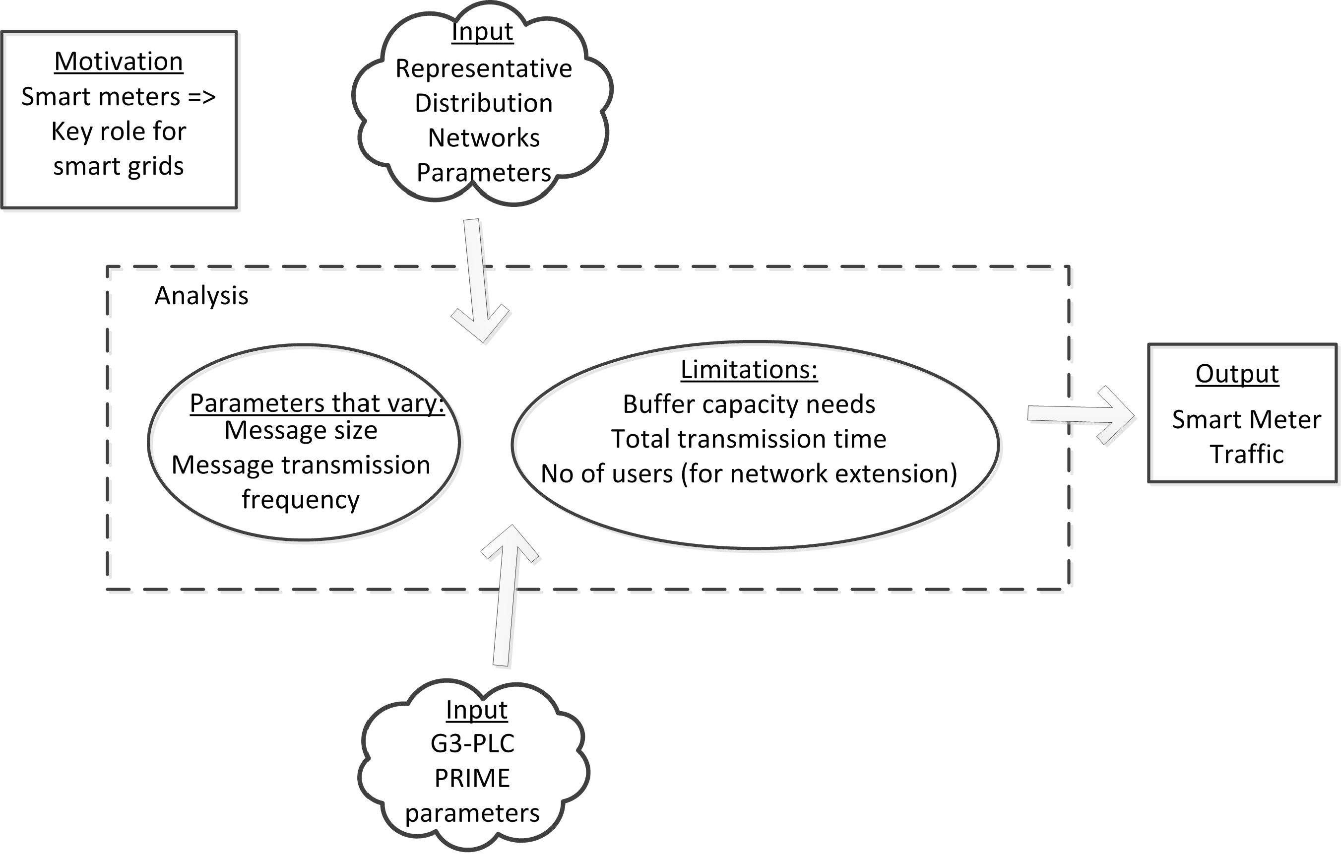
The modernization of the distribution grid requires a huge amount of data to be transmitted and handled by the network. The deployment of Advanced Metering Infrastructure systems results in an increased traffic generated by smart meters. In this work, we examine the smart meter traffic that needs to be accommodated by a real distribution system. Parameters such as the message size and the message transmission frequency are examined and their effect on traffic is showed. Limitations of the system are presented, such as the buffer capacity needs and the maximum message size that can be communicated. For this scope, we have used the parameters of a real distribution network, based on a survey at which the European Distribution System Operators (DSOs) have participated. For the smart meter traffic, we have used two popular specifications, namely the G3-PLC–“G3 Power Line communication” and PRIME–acronym for “PoweRline Intelligent Metering Evolution”, to simulate the characteristics of a system that is widely used in practice. The results can be an insight for further development of the Information and Communication Technology (ICT) systems that control and monitor the Low Voltage (LV) distribution grid. The paper presents an analysis towards identifying the needs of distribution networks with respect to telecommunication data as well as the main parameters that can affect the Inverse Fast Fourier Transform (IFFT) system performance. Identifying such parameters is consequently beneficial to designing more efficient ICT systems for Advanced Metering Infrastructure.

1. Introduction

The traditional electricity grid is undergoing significant changes and it is evolving to cope with the constantly growing technological demands. The necessity to reduce the CO₂ emissions and the need to accommodate an increasing number of RES (Renewable Energy Sources) implies that an effective energy management should take place. Therefore, the grid should be controlled and monitored through advanced ICT tools and it should be equipped with automatization devices. Apart from accommodating the energy from RES in the most effective way, the modern smart grid will be required to facilitate load-shifting on behalf of the utilities, to avoid load peaks, and to enable the recognition of faults or outages in an automatized way. In addition, a two-way communication between the utilities and the consumers is considered of vital importance, to achieve end-user awareness and an eventual consumption reduction [1].

Smart meters play a key role in the smart grid, since they can provide useful information about the consumption and the consumer profile, which can lead to load prediction and load peak reduction. Moreover, the energy provider can use such information for possible consumption control through load-shifting. On the other hand, the smart meters can be a useful interaction tool between the energy provider and the end user, via which the consumers can be actively involved in reducing their consumption [2].

Smart meters have been widely employed both for national roll-outs as well as for the realization of smart grid projects [3]. Overall, it is expected that until 2020 around 200 million smart meters will be deployed with an estimated investment of 35 billion € [4]. Due to the increased interest on smart metering applications, there has been a development of the technologies that support them. Smart meter data transmission is usually divided in two links: the first link carries data from the smart meter to a data concentrator whereas the second link connects this data concentrator to the control center of the energy provider [5]. There are several telecommunication technologies utilized by smart metering applications and they are mainly distinguished according to the transmission medium used for the signals, thus being divided into wired and wireless [5]. A popular wired smart meter technology is the PLC (Power Line Communication) and in particular the NB-PLC (Narrow-Band PLC), which is used mainly for the first transmission link. Two popular technological solutions for NB-PLC are the PRIME [6] and G3-PLC [7] specifications, which constituted the main basis for the standards proposed by ITU and IEEE [8]. Cellular technologies are usually preferred for the second transmission link.

There is significant feedback in the literature with respect to smart meter data communications networks, their characteristics, and their limitations. In [9] a real PRIME network is simulated, and network problems are studied. The correct functionality of the system is examined in [10] if PRIME smart meters from different vendors are used, whereas in [11] it is also examined if smart meters from different manufacturers interoperate correctly with data concentrators from different vendors. The identification of the distribution line and the substation at which each smart meter is connected are examined in [12]. The network configuration, where many smart meters are accommodated, is studied in [13], where also memory requirements are addressed with respect to the data traffic communicated. AMI networks are examined in terms of security requirements for communications in [14] whereas in [15] anonymization of smart meter data is studied, meaning that the utility receives some information, apart from billing data, without knowing to which smart meter it corresponds. All these prove the importance of the smart meter data communication solutions.

Smart meters are a key element of the smart grid and they enable important applications, such as demand response and energy management. Demand response refers to the actions taken to decrease the overall peak in consumption, for example by shifting or curtailing loads. It is an emerging technique and several studies have been done to address such issues. In [16], the authors examine smart residential energy scheduling with a two-stage mixed integer linear programming (MILP). In the first stage they obtain the optimum scheduling for appliances, whereas in the second stage they model the random behavior of the users. In [17] the scheduling of the appliances in a long-term perspective is examined and a Markov description process for the alterations in price and load demand is used. An online load scheduling learning (LSL) algorithm is developed, which decreases the peak-to-average ratio in the aggregate load. The Nash equilibrium in the one-shot game is examined in [18], where a DR repeated game is proposed instead, which can benefit both the energy provider and the customers. In this program, the set of users is divided into groups. Each group participates in the DR program in one period. In [19], the authors develop a load management method, which utilizes the multi agent systems to reduce the peak load of a smart distribution network feeder.

Due to the increasing number of smart meters being implemented and the growing amount of smart meter data requested by the energy providers, scalability issues with respect to the smart meter data traffic are of vital importance and have motivated our work, since the system needs to be able to process and store all this data properly. There are some studies found in the literature for this scope. In [20] an analysis has been made about the traffic added by smart meters to the cellular network and the equivalent signaling overhead. The limitations of a cellular Wide Area Network (WAN) for smart meter traffic are addressed in [21], whereas a bandwidth analysis of the smart meter network infrastructure depending on the traffic sent is carried out in [22]. In [23] information is given about latency and data rates required by smart metering applications. The delay and packet loss ratio for smart grid control traffic are examined in [24]. Methods for reducing the volume of traffic are studied in [25,26] through packet concatenation or aggregation methods at the data concentrator before the data is forwarded to the control center. In [27] the data traffic in selected system nodes, such as the smart meter or the data center firewall, is examined. In [28] scalability issues are examined with respect to the transmission time needed for several smart meters and several data concentrators that transmit data.

In this work we examine the smart meter data traffic that is communicated up to the data concentrator in a real distribution system and all the parameters of such a system are considered. A real distribution network and its characteristics have never been examined—to the best of our knowledge. In our analysis we considered the aforementioned literature for the smart meter message size and the message transmission frequency that can be found. Specifically, information about the message size is found in [20,21,23,24,25,26,27,28], whereas information about the message transmission frequency is found in [13,23,25,26,27]. It should be noted that when the PLC technology is implemented, the data concentrator is usually positioned within the substation. The data traffic is directly connected to the number of consumers that exist on the LV distribution system. In [29] a study has been performed with respect to the LV distribution grid in Europe. The work has been based on a survey at which the European DSOs (Distribution System Operators), which represent the 74.8% of the consumers in total, have participated. Based on this survey, the mean values for the characteristics of a representative network have been derived. In this work, the data traffic has been studied based on these values, i.e., the number of consumers, the distance of the consumers to the substation, for three representative LV networks, the urban, the semi-urban and the rural network.

In our analysis, we simulated the traffic arriving at the data concentrator if the G3-PLC or the PRIME solution is used as the telecommunication techniques. These technologies are used, since they are both the most popular methods used widely in practice. The physical layers have been simulated and all the parameters are considered to derive the number of G3-PLC or PRIME frames needed for a specific message size for transmission. Since there is a great diversity in the literature referring to the message size and the frequency under which these messages are sent by the smart meter, we have considered various values for these parameters. The diversity could be because the message size and the frequency of transmission depend highly on the way smart meter data are planned to be used by the energy provider, which is by definition a procedure that alters according to current needs. Further on, we have examined limitation factors of the system. To be more precise, we have studied the effect of the total transmission time on the maximum message size that can be sent by the smart meter, along with the effect of the total buffer size to this smart meter message size. For reasons of completeness, we also examined the maximum number of users that could be handled by the system for a specific message size and frequency, provided that the number of users is not given by the representative networks. This study could be useful, in case a distribution network needs to expand and accommodate more consumers.

In general, the contributions of this paper can be summarized as follows:

• Smart meter traffic is examined in a real distribution network; the parameters of such a network are considered.
• Two popular telecommunication techniques are considered for the traffic analysis, namely the PRIME and G3-PLC specifications.
• Variable values are considered for the message size and the transmission frequency, which respect the available literature review.
• Limitations of the system are considered, such as a finite buffer size, a maximum message size that can be transmitted.
• Possible expansion of the number of customers accommodated by a distribution network is examined, and its respective limitations.

The rest of the paper is organized as follows. Section 2 gives the characteristics of the G3-PLC and PRIME technologies that are used. In Section 3 the traffic analysis is presented along with the parameters of a representative distribution network, whereas in Section 4 limitations are discussed with respect to the buffer capacity needs, the total transmission time needed, and the number of users supported (if the distribution networks need to be expanded). Section 5 concludes the paper.

2. NB-PLC Technologies

2.1. System Based on G3-PLC

As it has been mentioned in Section 1, to simulate the traffic arriving at the Data Concentrator from a real distribution network, the G3-PLC and PRIME technologies are used. These two solutions are selected because it has been proved that they are widely used in practice [3]. The G3-PLC characteristics presented here are described in [7]. G3-PLC specifies seven frame lengths. In this work, we use 3 of those frame lengths to test the system’s performance.

Table 1. Arrangement of Data in Frames Based on G3-PLC.

Number of OFDM Symbols (NS)	RS Encoder: Input/Output Symbols	Convolutional Encoder: Input/Output Bits	Max Encoded Bits in Each Frame	Data Bits in Each Frame
112	235/251	2014/4028	4032	1880
40	73/89	718/1436	1440	584
12	10/26	214/428	432	80

shows the lengths of the frames used and their size at various stages of the encoding procedure. It is assumed that the data undergoes concatenated encoding with Reed Solomon codes to be applied to information data, where one symbol is formed out of 8 bits, and convolutional encoding to follow with a coding rate of ½ and a constraint length L_c = 7. It should be noted that six zeros are added to terminate the convolution encoder state to all-zeros state. It is also assumed that the symbols are modulated with DBPSK modulation. Further on, the OFDM method is used for transmission, meaning that higher data rates can be achieved thanks to multicarrier transmission. The OFDM transmission is realized through a 256-point IFFT (N_ifft = 256). However, only 36 carriers transmit useful information, whereas the rest are null carriers. The OFDM symbols to be transmitted are defined as follows:

$$x_w\left(q\right)={\displaystyle \sum _{y=0}^{N_c-1}{b}_y\left(q\right)\cdot e^{j\cdot \left(\raisebox{1ex}{$2\pi $}\!\left/ \!\raisebox{-1ex}{${{\rm N}}_c$}\right.\right)\cdot y\cdot w}}$$

(1)

The parameter N_c is the number of carriers, b_y is the y-th bit in the BPSK modulated symbol included in the q-th OFDM frame and x_w is the w-th sample of the transmitted sequence.

The frequencies of the first and last useful carrier are f_u1 = 42 and f_u2 = 88.848 kHz respectively and they belong to the CENELEC A band. The frequency spacing between carriers is Δf = 1.5625 kHz, whereas the sampling frequency is F_S = 400 kHz. A cyclic prefix of N_CP = 30 samples is used to mitigate the effect of intersymbol interference, whereas the samples that undergo overlapping are N_O = 8. The frame to be transmitted consists not only of the encoded information bits but also of a Frame Control Header (FCH), which includes information about the type of the frame, and the preamble part. The FCH bits are not subject to Reed Solomon encoding but only to convolutional code, robust mode 6, meaning that the encoding is repeated 6 times bit by bit. The total number of FCH bits is 33, which leads to several symbols being transmitted, N_FCH = 13. The preamble consists of 8 identical P_p symbols and 1.5 identical M_p symbols, each of which contains 256 samples (N_ifft) that are transmitted right before the data symbols. Thus, the preamble symbols are N_pre = 9.5. The duration of the frame is calculated through (2):

$$T_{Frame}=\left(\left(N_S+N_{FCH}\right)\cdot \left(N_{CP}+N_{ifft}-N_O\right)+\left(N_{Pre}\cdot N_{ifft}\right)\right)/F_S$$

(2)

where N_S is the number of OFDM symbols to be transmitted. From (2) it can be deduced that the number of samples to be transmitted is:

$$N_{samples}=\left(\left(N_S+N_{FCH}\right)\cdot \left(N_{CP}+N_{ifft}-N_O\right)+\left(N_{Pre}\cdot N_{ifft}\right)\right)$$

(3)

Since Differential Binary Phase Shift Keying (DBPSK) modulation is used in the system, one sample corresponds to one bit.

2.2. System Based on PRIME

For simulating the traffic arriving at the data concentrator provided that the PRIME technology is used, the characteristics described in [6] are used. It is assumed that a convolutional encoder is used with a coding ratio of ½ and a constraint length L_c = 7. DBPSK modulation is used further on. In this work, three frame sizes are used to test the system’s performance.

Table 2. Arrangement of Data in Frames Based on PRIME.

Number of OFDM Symbols	Convolutional Encoder: Input/Output Bits	Max Encoded Bits in Each Frame	Data Bits in Each Frame
39	1872/3744	3744	1866
12	576/1152	1152	570
2	96/192	192	90

shows these frame sizes used along with the frame lengths at each stage of their processing. Again, six zeros are added to terminate the convolution encoder state to all-zeros state.

The symbols are transmitted through the OFDM method. The OFDM symbols are defined as in (1) before they are transmitted through the NB-PLC channel. For the OFDM transmission a 512-point IFFT is used (N_ifft = 512), but only 96 carriers are used for data transmission, plus one pilot carrier. The frequencies used are in the CENELEC A band and it is f_u1 = 42 and f_u2 = 88.848 kHz respectively. The frequency spacing between carriers is Δf = 488 Hz and a cyclic prefix of 48 samples (N_CP = 48) is used for dealing with intersymbol interference. The duration of the cyclic prefix is T_CP = 192 μsec. Apart from data to be transmitted, the PRIME frame consists of a 2-symbol Header (N_H = 2) and the preamble. Each symbol has a duration of T_symbol = 2.24 msec, whereas the preamble has a duration of T_preamble = 2.048 msec and the total number of OFDM symbols to be transmitted is N_S. Thus, the total duration of the frame is given by (4):

$$T_{Frame}=(\left(N_S+N_H\right)\cdot 2.24\cdot {10}^{-3}+2.048\cdot {10}^{-3})$$

(4)

3. Traffic Analysis—Results

3.1. Parameters of Representative Distribution Networks

In this work we describe the traffic produced by smart meters that can be experienced in reality. Therefore, the parameters that describe a real distribution network are considered. In [29] an extensive analysis has been carried out about the distribution networks in Europe and the main parameters describing them. Among others, it is defined, how many LV consumers exist per MV/LV substation, the average LV circuit length per consumer, the transformer capacity and the area that is covered by each substation. The distribution networks are categorized into urban, semi-urban and rural ones with respect to the area that they cover. Therefore, our analysis about the traffic arriving to a data concentrator follows this classification of urban, semi-urban and rural networks.

According to [29], the average number of consumers per substation is N_u = 101, N_su = 87, N_r = 51 for an urban, a semi-urban and a rural area respectively. Another interesting parameter is the average distance between the consumer and the substation, which serves for estimating the data transmission time to the substation. This parameter can be derived by the average area that is covered by each substation, if this area corresponds to a circular surface. We also assume the worst-case scenario, where the substation and consequently the data concentrator will be positioned at the far end of the considered area. Therefore, for an average area of E_u = 0.5, E_su = 1.5 and E_r = 2.64 km², for an urban, a semi-urban and a rural area respectively, we get for the average distance between the consumers and the data concentrator D_u = 398, D_su = 691 and D_r = 917 m.

3.2. Parameters for Traffic Analysis

In this Section an analysis of the traffic that arrives at the data concentrator under realistic conditions is presented. For representing these realistic scenarios, the characteristics of the representative urban, semi-urban and rural distribution networks have been used.

First, we examine the total time that would be required so that all consumers transmit a data message to the data concentrator to which they are linked. The transmission time for each consumer calculated here is based on the payload to be transmitted and the time needed for the data to be transferred through the power line from the consumer to the data concentrator. The total transmission time is calculated by summing the transmission time for all customers that can be accommodated by one data concentrator:

$$T_{total}={\displaystyle \sum _{i=1}^{N_c}\left[\left(T_{frame}\cdot N_{frames}\right)+\left(D_c\cdot \sqrt{{\epsilon }_r}\right)/c_0\right]}$$

(5)

where T_frame is given by (2), N_frames is the number of frames required to transmit the message data in total, ε_r is the dielectric constant of the power lines, c₀ is the speed of light and N_c and D_c can be equal to N_u, N_su, N_r and D_u, D_su, D_r respectively depending on the type of area under examination.

To calculate the total number of G3-PLC or PRIME frames that needs to be transmitted, the size of each message packet for transmission needs to be defined. There can be found several values in the literature for the message packet size sent by the smart meters to the data concentrator. For example, in [26] it is defined that a typical smart meter message size is around 150 bytes. In [25] it is mentioned that the message can be from 20 to 500 bytes and that a few kb of data is sent to the grid operator. According to [24] the message size can vary from 70 to 750 bytes, whereas the message size gets values from 25 to 2133 bytes in [21]. In [27] it is mentioned that the average traffic per day is 3185 bytes. The message size varies from 4 to 40,000 bytes in [20], whereas according to [28] the maximum message size can be as high as 145,888 bytes. In [23] a typical smart meter message size is around 100 bytes and the traffic sent to the data concentrator can vary from 1600 to 2400 bytes per reading interval.

In general, the message packet size can vary a lot depending on the type and amount of data that the energy provider needs. For simple functions such as remote reading of consumption, a small message packet size could be sufficient, whereas for sophisticated functions, such as deriving consumption profiles and identifying the type of electrical devices that are switched on in a particular moment, more data is required. Therefore, the more automated and smart the grid becomes, the more the demand increases for providing detailed and accurate data. Consequently, the data traffic is expected to increase, with the employment of more smart meters and the grid development.

Another parameter that is of great importance is the frequency at which a smart meter transmits to the data concentrator. Similar to the message size, the frequency at which the messages are sent can vary a lot. For example, in [27] it is mentioned that the smart meters transmit 3 times per day. In [25,26] it is defined that a small message is sent every 15–60 min to the data concentrator. In [13] high frequency rates are examined with messages being sent even every 5 or 10 min. In [23] it is defined that the reading messages are sent 4 or 6 times per day from every smart meter and they represent information recorded by the smart meter every 15 min.

The frequency at which the messages are sent to the data concentrator depends highly on the application planned from the energy provider. If close to real time information is needed, then short messages will be required very frequently. For more delay-tolerant applications, data can be transmitted a few times per day from each smart meter and the information included can represent more detailed or frequent recordings. As a first step, we examine the traffic arriving at the data concentrator if each smart meter transmits a fixed number of times per day, namely 4, 6, 8 and 24 times per day. A variable message size is used for the simulations. In the following sub-section, we examine the traffic in relation to the frequency at which the messages are sent, whereas certain fixed message sizes are used.

3.3. Traffic Analysis for G3-PLC Based on the Message Packet Size

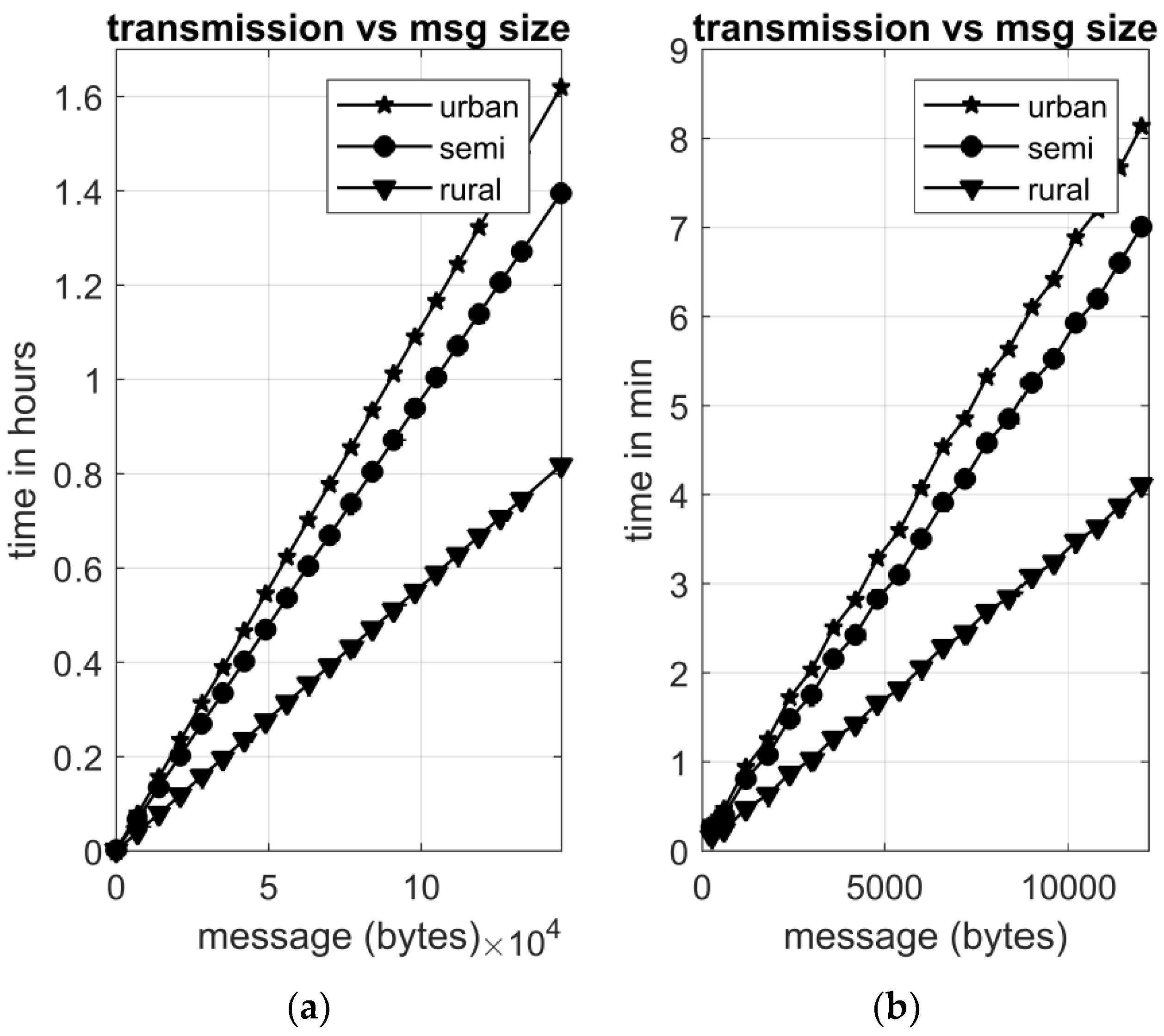
The traffic that can reach the data concentrator is simulated by utilizing the characteristics of the G3-PLC technology. Several message sizes have been used. According to the values found in the literature, we firstly used a variable size from 4 to 145,888 bytes to cover the entire range of possible message sizes. As a next step, we examined the traffic created for a shorter range of message size, which represents a more common scenario. Figure 1 shows the time that would be required for all the data to be transmitted to the data concentrator, calculated according to (5) and by using a 112 OFDM symbol data frame. The variable defining the number of frames needs to be calculated for every different message size considering the G3-PLC characteristics. Different message sizes can result in the same number of frames to be transmitted, since the number of data bits for each frame is determined by the G3-PLC features. Therefore, although Equation (5) has a linear form, the transmission time curves show a quasi linear form, which becomes more obvious when the range is small. With a large range of message sizes, this non-linearity is not that obvious. However, the results for both ranges give a clear picture of the transmission time required for the data to be transmitted. The three curves represent the cases where an urban, a semi-urban and a rural area are taken into consideration. The transmission time assumes that each smart meter transmits after the other with perfect synchronization. Therefore, the transmission time depicted is the best-case scenario that could be encountered. In reality, this transmission time is greater due to gaps between transmission and non-perfectly synchronized clocks.

As it is expected, the time needed for transmission increases dramatically for very high message sizes. It can be observed that for a very small message size of 4 bytes, the time required can be as small as 9.4 s for the urban case scenario, whereas for a huge message of 145,888 bytes the necessary time equals to 1.62 h. In

Table 3. Transmission Time for Certain Message Sizes (112 OFDM Symbol Data Frame).

Message (Bytes)	100	258	1600	3200	4128	6192	8256
Ttotal in urban area	9.4 sec	18.8 sec	65.7 sec	2.19 min	2.82 min	4.23 min	5.63 min
Ttotal in semi-urban area	8.1 sec	16.2 sec	56.6 sec	1.89 min	2.43 min	3.64 min	4.85 min
Ttotal in rural area	4.7 sec	9.5 sec	33.2 sec	1.1 min	1.42 min	2.13 min	2.85 min

the total transmission time is shown for some message packet sizes that have been found to be used in the literature. For example, a message of 258 bytes needs 18.8 sec to be transmitted from all smart meters in an urban area, while a message of 3200 bytes would need 2.19 min.

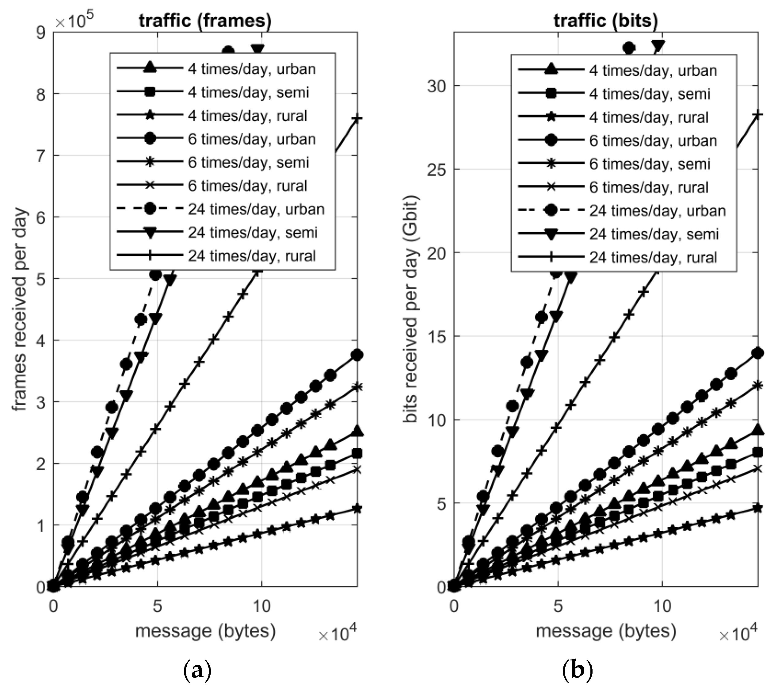
Figure 2 shows the frames and the bits received at the data concentrator versus the message size which varies from 4 to 145,888 bytes for the urban, semi-urban and rural environment, when the messages are transmitted every 1, 4 or 6 h. It should be noted that not all points depicted in the figure represent realistic scenarios. For instance, it is rather unlikely that a smart meter will be required to transmit a large message of 145,888 bytes every hour or that a message of 4 bytes sent 4 times per day would be enough for the grid operator to perform all the desirable applications. However, the graph gives a good picture of the traffic that needs to be accommodated from a real distribution network. It should also be noted that for the urban and semi-urban scenario, certain amounts of traffic cannot be accommodated throughout a day, because their transmission time would exceed the duration of 24 h. This case is depicted in Figure 2, namely traffic over 104,575 and 90,005 kbytes for the urban and semi-urban case respectively cannot be dealt with.

It can be noted that a very small message size of 4 bytes results in 25.8 kbits of data to be processed daily if the message is transmitted every 4 h for the urban scenario. This means that 808 frames arrive to the data concentrator per day, leading to 30 Mbits received per day according to (3). The equivalent values are 943 Mbits of data, 501,768 frames and 18.66 Gbits received daily for a message of 145,888 bytes.

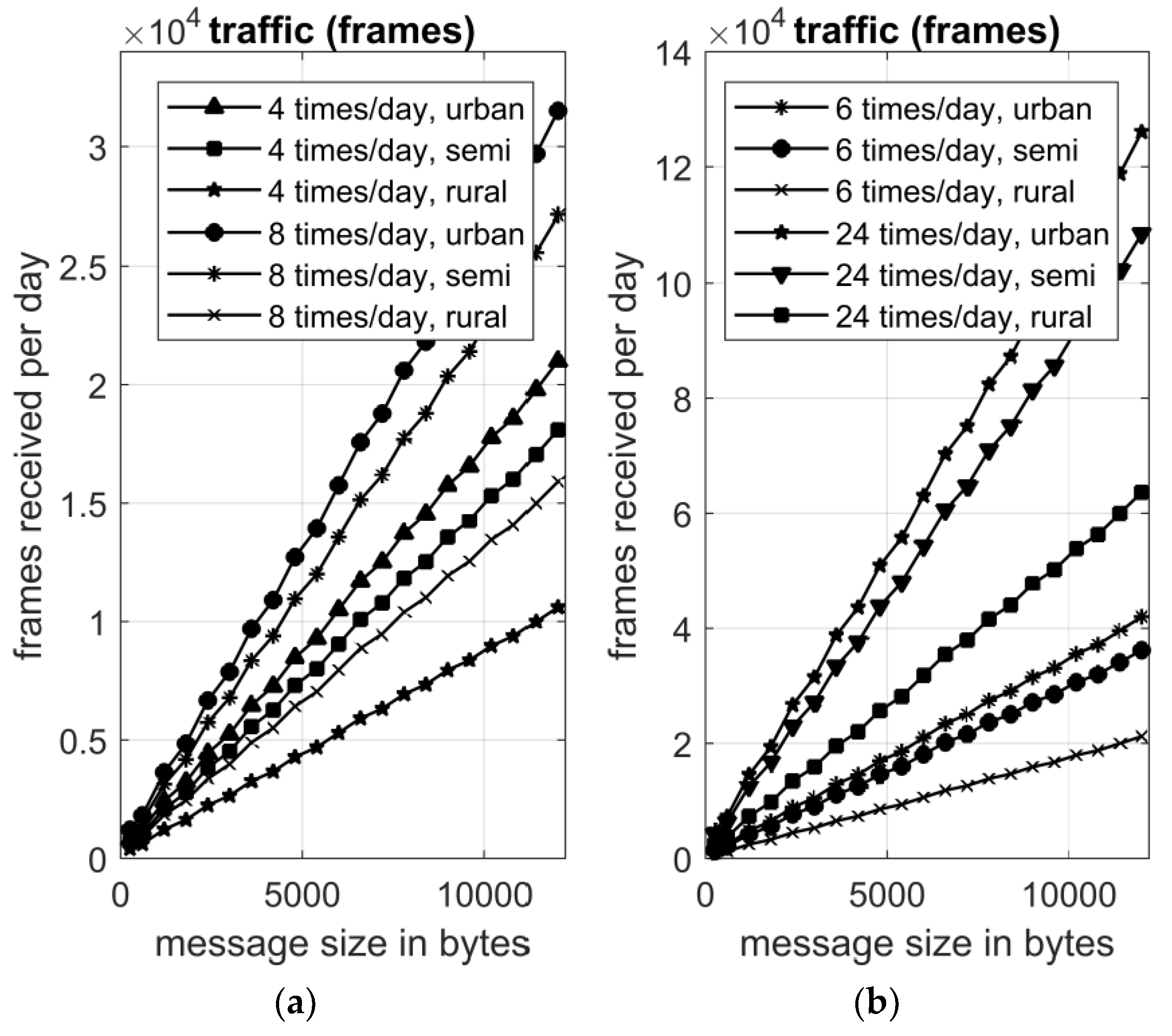
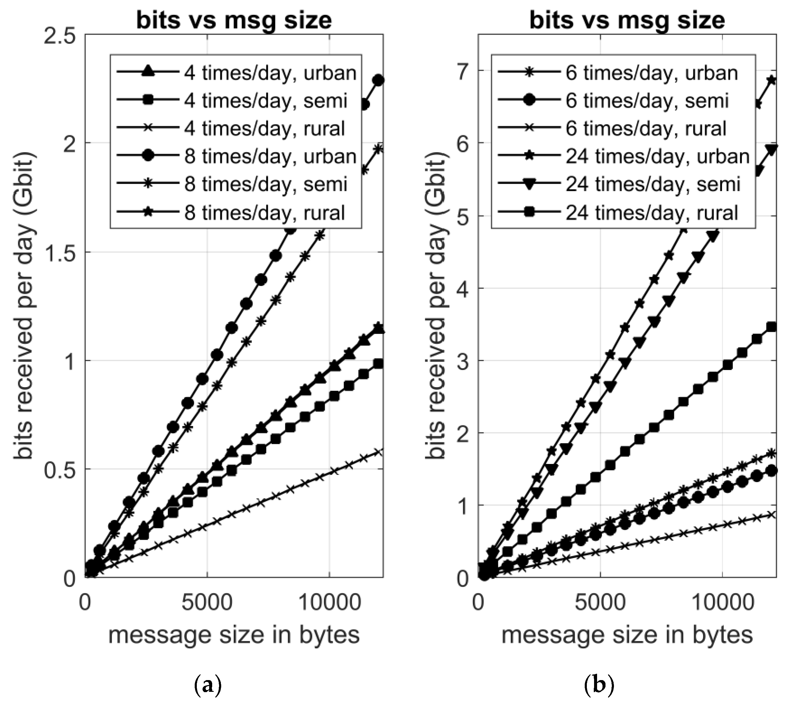
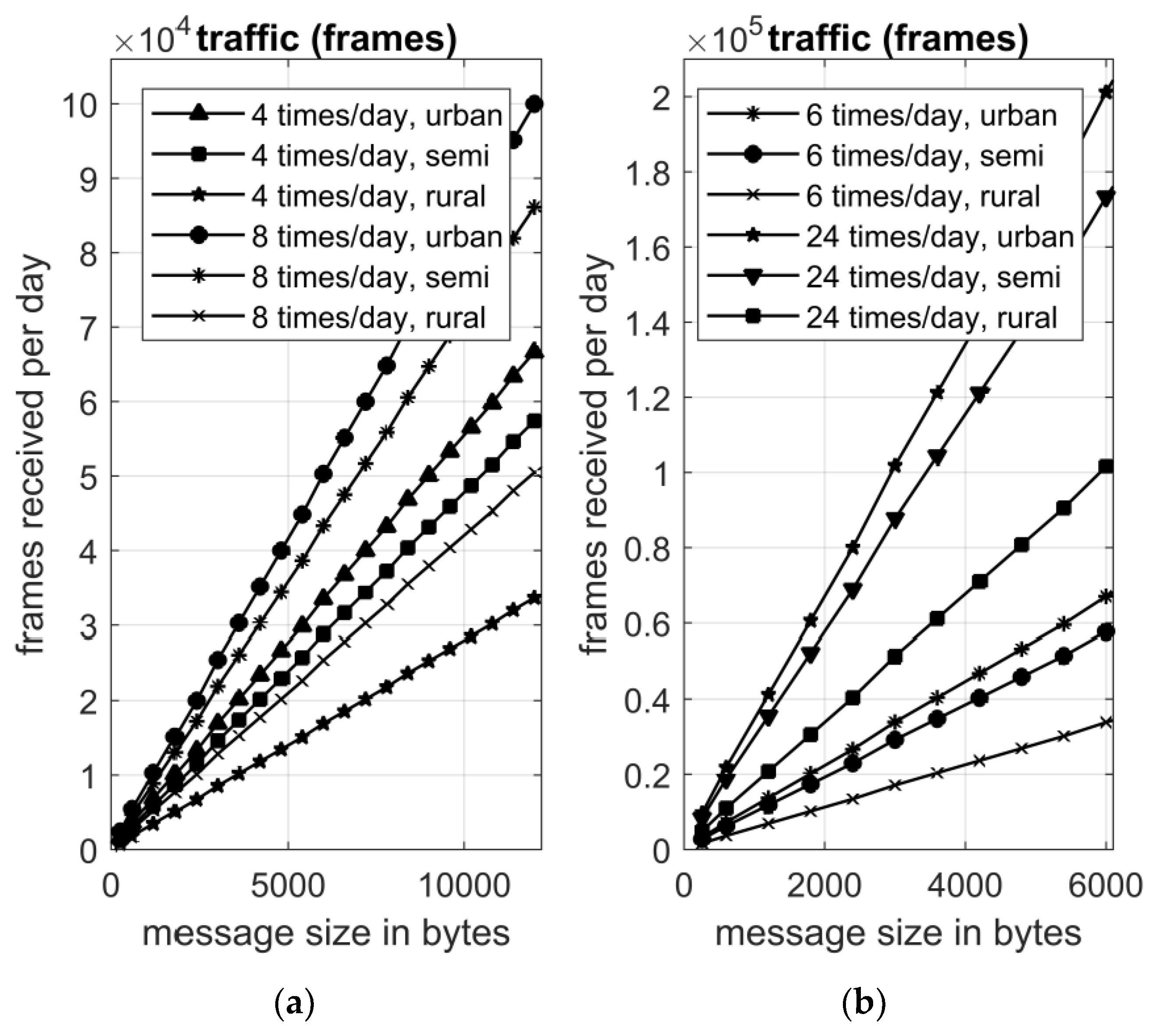
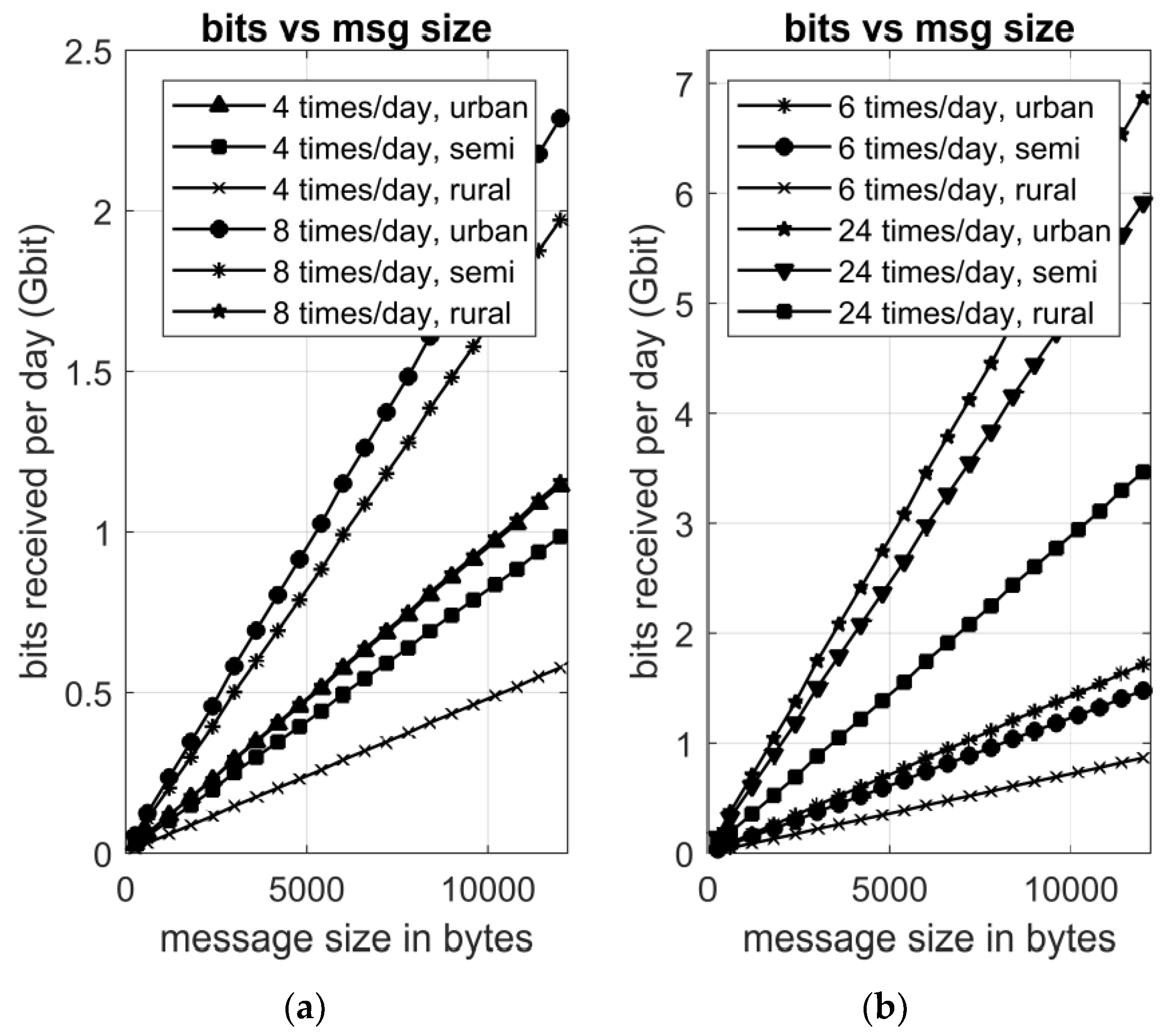
Figure 3 and Figure 4 depict the frames and the data bits received by the data concentrator when a shorter range of message size is used. The message size varies from 258 to 12,000 bytes and the figures show in a more detailed way the traffic resulting from realistic message size scenarios. The figures show 4 different frequencies at which the data is sent to the data concentrator, namely 4, 6, 8 and 24 times per day. It can be observed, that for a message size of 2400 bytes for the urban scenario, 11.63 Mbits of data are needed to be processed, whereas the equivalent traffic arriving at the data concentrator is equal to 6666 frames and 247.86 Mbits. For a message size of 8256 bytes the respective values are 40.03 Mbits of data, 21,816 frames and 811.16 Mbits received daily.

Figure 3 and Figure 4 show that the curves are quasi linear, as explained before. The graphs allow the reader to have a clear picture of the traffic that needs to be handled at the data concentrator for different message sizes.

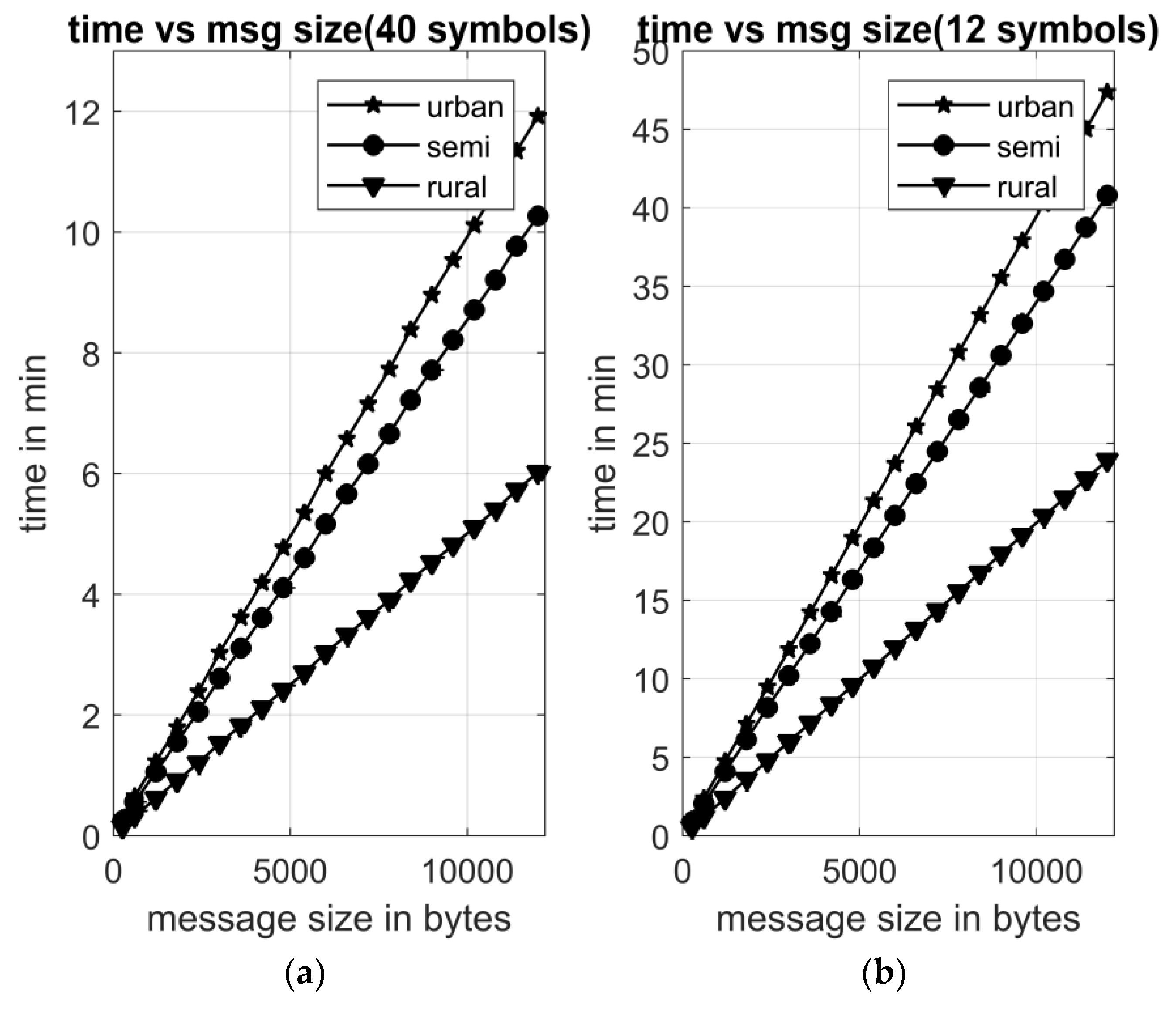
Figure 1, Figure 2, Figure 3 and Figure 4 refer to the traffic analysis when a 112 OFDM symbol frame is used for transmission. To complete the picture of a realistic distribution network and the smart meter traffic it creates, we examine the case where smaller frame sizes are used from the G3-PLC specification. For this reason, a medium and a small frame size of 40 and 12 OFDM symbols is used. This part of the analysis completes the picture of the traffic required to be handled, and it shows that the selection of the G3-PLC characteristics can have an impact on the overall resulting traffic. We present the case where the message size to be transmitted varies from 258 to 12,000 bytes. Figure 5 shows the transmission time that would be required for the data of all smart meters to be transmitted to the data concentrator, with the aforementioned message size range and provided that 40 and 12 OFDM symbols are used instead of 112. In this case, the big OFDM symbol size is replaced with a medium and small one and the transmission time required is illustrated. It is again examined the case of an urban, a semi-urban and a rural area. Transmission implies perfect synchronization among smart meters and thus no gaps between consecutive transmissions. In

Table 4. Transmission Time for Certain Message Sizes (40 OFDM Symbol Frame).

Message (Bytes)	100	258	1600	3200	4128	6192	8256
Ttotal in urban area	8.7 sec	17.3 sec	1.6 min	3.2 min	4.1 min	6.1 min	8.2 min
Ttotal in semi-urban area	7.5 sec	15 sec	1.37 min	2.7 min	3.5 min	5.3 min	7.1 min
Ttotal in rural area	4.4 sec	8.8 sec	48.15 sec	1.6 min	2.1 min	3.1 min	4.2 min

and

Table 5. Transmission Time for Certain Message Sizes (12 OFDM Symbol Frame).

Message (Bytes)	100	258	1600	3200	4128	6192	8256
Ttotal in urban area	23.7 sec	61.6 sec	6.3 min	12.6 min	16.3 min	24.5 min	32.6 min
Ttotal in semi-urban area	20.4 sec	53 sec	5.4 min	10.9 min	14 min	21.1 min	28.1 min
Ttotal in rural area	12 sec	31.1 sec	3.2 min	6.4 min	8.2 min	12.4 min	16.5 min

the total transmission time is showed for some message packet sizes that have been found to be used in the literature in case the 40 or the 12 OFDM symbol frame is used.

As it can be observed from Figure 5 and Table 4 and Table 5, the total transmission time is a bit inferior when 40 OFDM symbols are used with respect to the 112 OFDM symbol case for small message sizes. However, as the message size increases, the total transmission time increases a lot when fewer OFDM symbols are used. For example, with a message size of 6192 bytes, the total transmission time for the urban scenario is 4.23 min for the large OFDM frame, whereas this value is 6.1 min and 24.5 min for the 40 and 12 OFDM symbol frame. This is mainly because with the small symbol frame, more frames are required to transmit the same amount of information, thus resulting in greater transmission time.

Figure 6, Figure 7, Figure 8 and Figure 9 show the total number of frames and the bits that arrive at the data concentrator when the medium and small G3-PLC frame sizes are used, and the messages are transmitted every 1, 3, 4 and 6 h. It should be noted that the data bits that need to be processed are the same for all possible G3-PLC frame sizes since the message size to be transmitted remains unchanged. As it can be noticed from Figure 6 to Figure 9, the general trend is that for a greater message size we get a bigger number of frames and bits received. For example, for a message size of 8256 bytes sent every 1 h with the 112 OFDM symbol frame, the bits and frames received at the data concentrator for the urban scenario are 3.24 Gbit and 87,264 respectively. The equivalent values for the 40 and 12 OFDM symbol frame are 4.74 Gbit, 276,336 frames and 18.8 Gbit, 2,002,224 frames. However, for small message sizes, this is not the case. For a message size of 100 bytes sent every hour, we get 90 Mbit, 83 Mbit, 227 Mbit and 2424, 4848, 24,240 frames for the 112, 40 and 12 OFDM symbol frame respectively. A reason behind this could be that with a small message size, the big OFDM frames are not utilized in the best possible way, meaning that many carriers could be null carriers. This leads in having more big frames and thus more bits received.

3.4. Traffic Analysis for G3-PLC Based on the Message Transmission Frequency

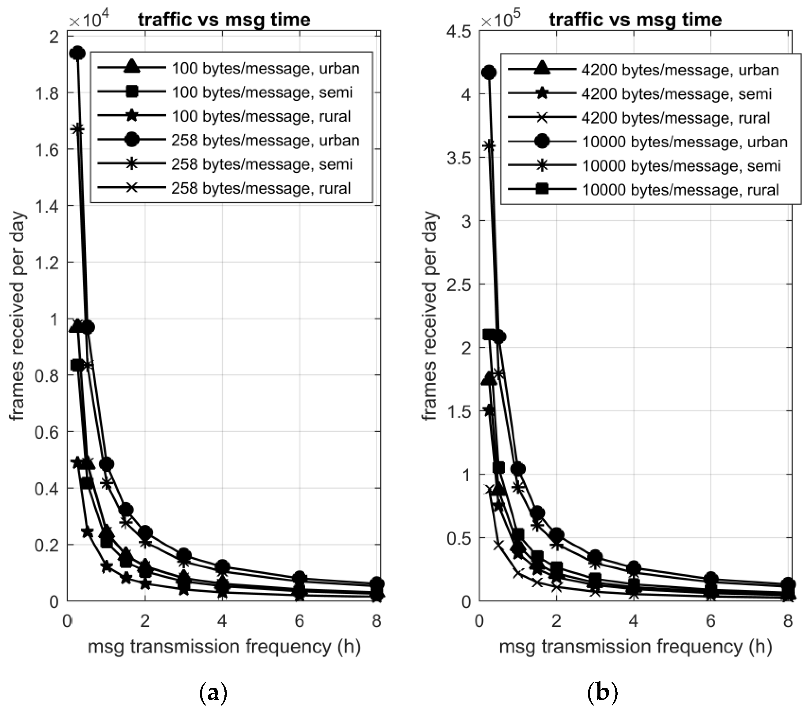
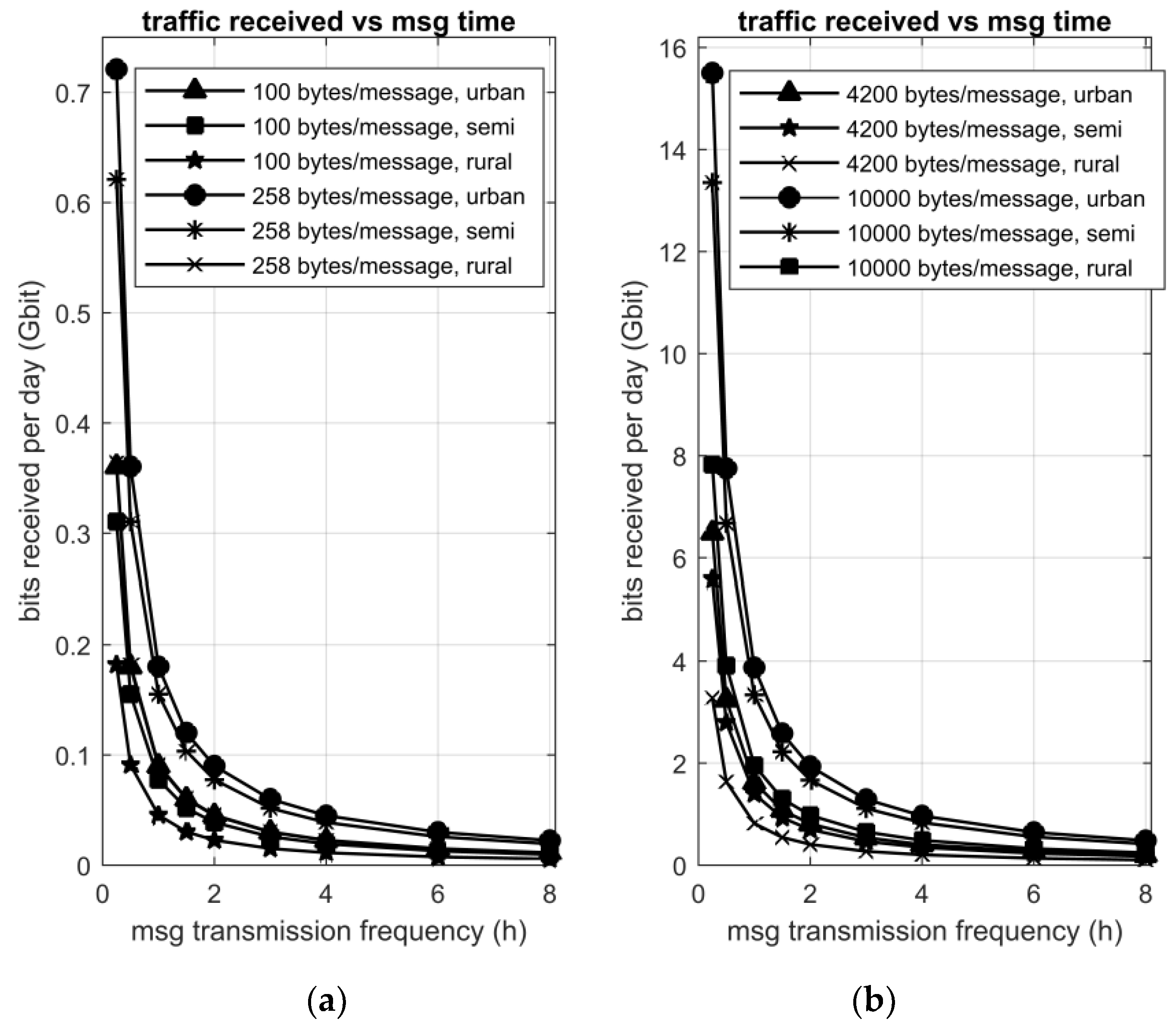
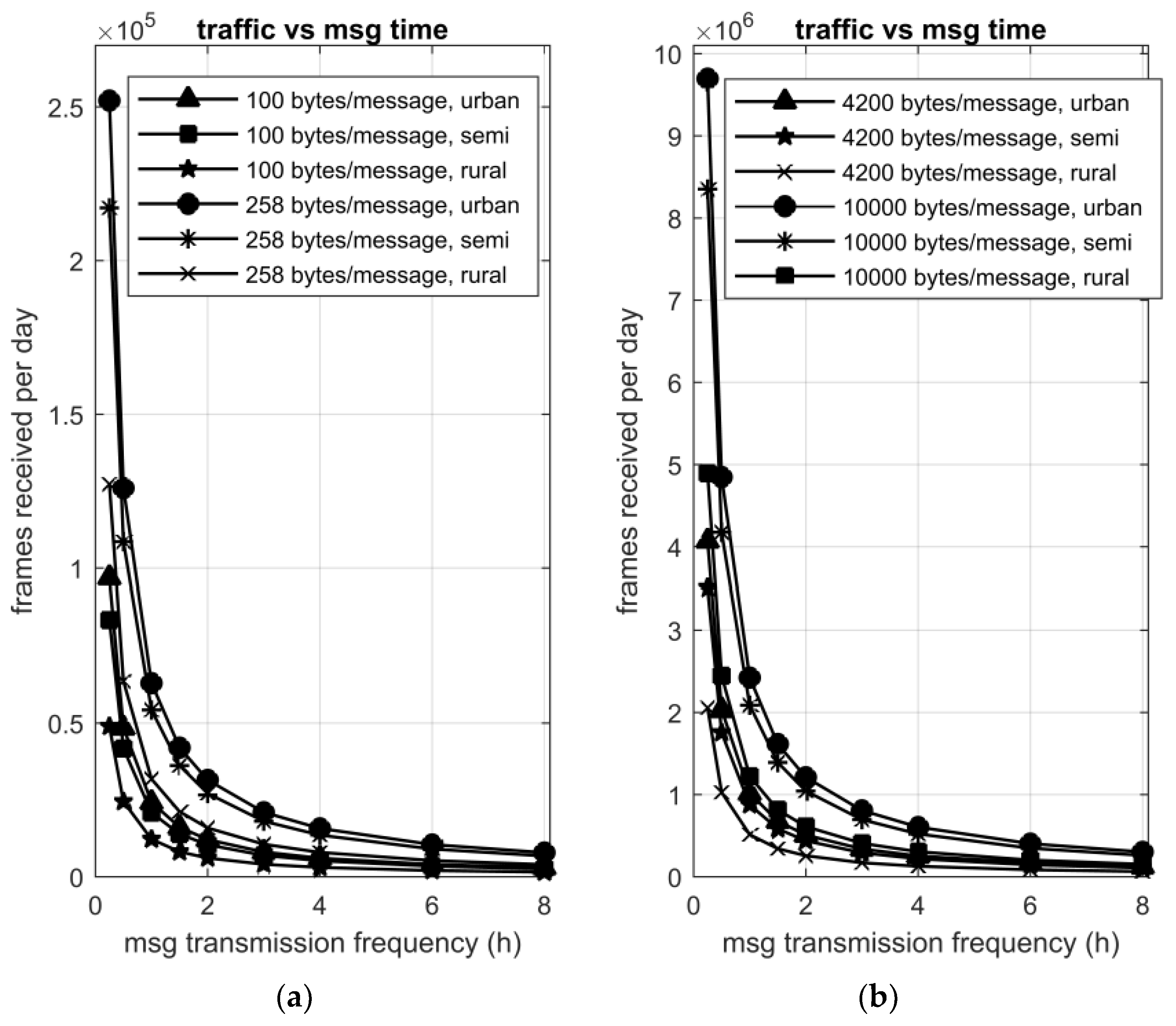
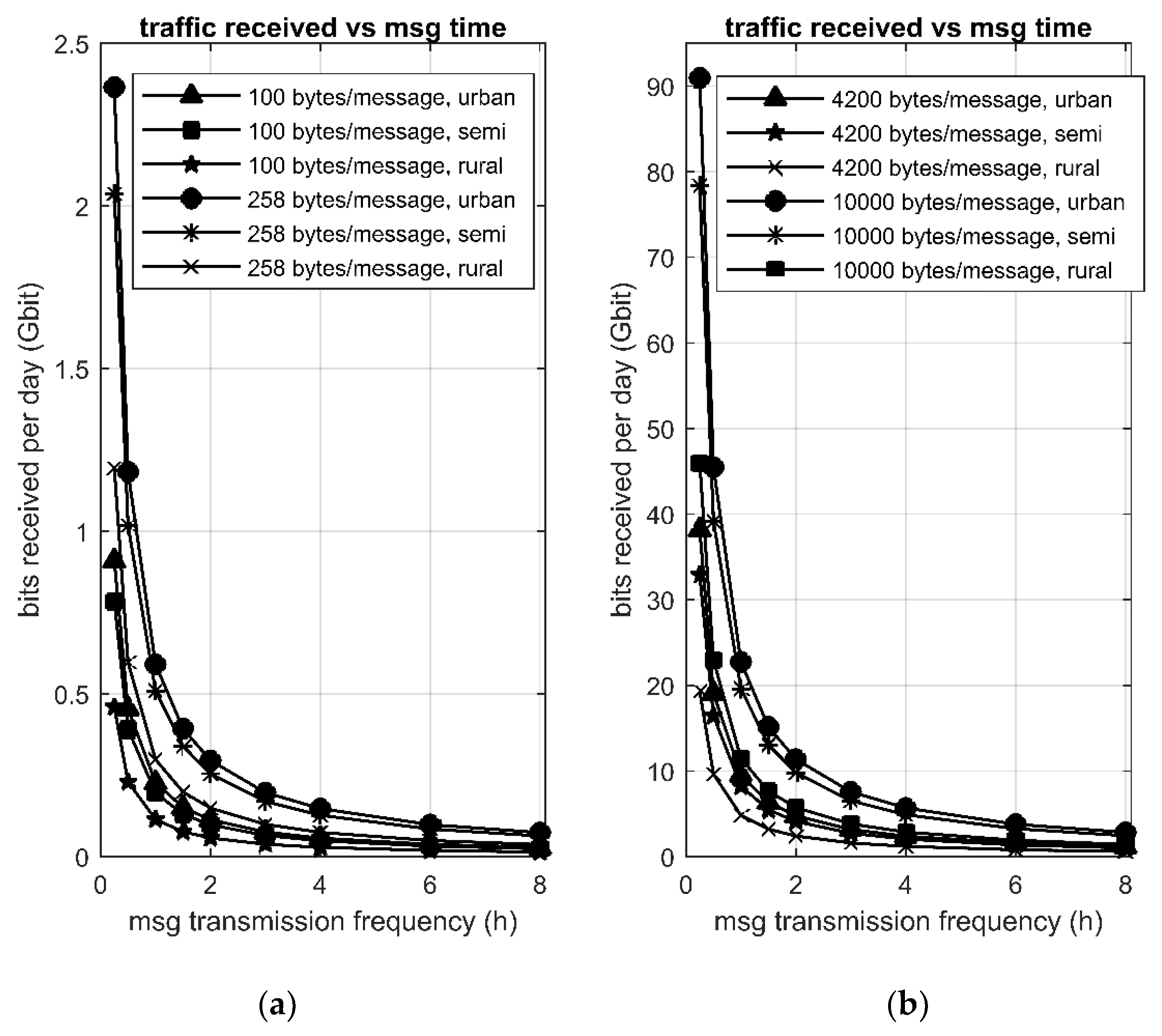
In this subsection we examine the traffic arriving at the data concentrator when different message transmission frequencies are used. We simulate the frequency at which the smart meter messages are sent from 15 min to 8 h. The message size to be transmitted is fixed to 100, 258, 4200 and 10,000 bytes, while the urban, semi-urban and rural cases are examined. Figure 10 and Figure 11 show the total number of frames and the bits received at the data concentrator when a 112 OFDM symbol frame is used. Figure 12 and Figure 13 show the traffic in terms of frames and bits when a medium OFDM frame size is used (40 symbols), whereas Figure 14 and Figure 15 show the equivalent values with a small OFDM frame size (12 symbols).

As it is expected, when the messages are sent more frequently, the frames and the bits that the data concentrator receives increase exponentially. The data bits for all OFDM data frame sizes are the same, since the message size examined remains the same for the 3 frame sizes examined. As a general trend, it can be noticed that the bits arriving at the data concentrator are increased with a smaller OFDM symbol frame. However, the 40 OFDM symbol frame results in less traffic arriving at the data concentrator than the 112 OFDM symbol frame for a message size of 100 and 258 bytes. The reason for this could be that these small message sizes may not be accommodated in the best way in the large OFDM frame, leading to null carriers, whereas they can be better accommodated in the medium OFDM frame size. On the other hand, the smallest OFDM frame is very likely to introduce great overhead, thus increasing the total number of bits received. For example, for a message size of 258 bytes sent every 15 min from the smart meters, the traffic arriving at the data concentrator results in 721, 665.8 and 2365.2 Mbit for a 112, 40 and 12 OFDM symbol frame size. For a message of 4200 and 10,000 bytes sent every hour the traffic arriving at the data concentrator is 1.6 and 3.88 Gbit (112 OFDM symbol frame), 2.4 and 5.7 Gbit (40 OFDM symbol frame), 9.55 and 22.7 Gbit (12 OFDM symbol frame).

3.5. Traffic Analysis for PRIME Based on the Message Packet Size

Apart from the traffic arriving at the data concentrator when the G3-PLC technology is used, the equivalent traffic is examined when PRIME is used. The rest of the simulation parameters with respect to the representative distribution networks are kept the same. A variable message size is also used, whereas the number of OFDM symbols that form a PRIME frame is according to Table 2. These frame sizes result in similar frame sizes with the G3-PLC case; thus, a better comparison can take place. It should be noted that since the message size to be transmitted is kept the same as in the G3-PLC case, the information bits arriving at the data concentrator will be the same also for the PRIME case. However, the total traffic as well as the total transmission time can vary, since this information data is divided in a different way into the frames to be transmitted.

Table 6. Transmission Time and Traffic for Certain Message Sizes (39 OFDM Symbol Frame).

Message (Bytes)		100	258	1600	3200	6192	8256
Transmission time	Turban	9.5 sec	19 sec	66.4 sec	2.2 min	4.3 min	5.7 min
	Tsemi	8.2 sec	16.3 sec	57.2 sec	1.9 min	3.7 min	4.9 min
	Trural	4.8 sec	9.6 sec	33.5 sec	67 sec	2.2 min	2.9 min
Traffic–Nbits, 4 times	Nb-urban	9.3 Mb	18.5 Mb	64.9 Mb	129.8 Mb	250.4 Mb	333.9 Mb
	Nb-semi	8 Mb	16 Mb	55.9 Mb	111.9 Mb	216Mb	288 Mb
	Nb-rural	4.7 Mb	9.4 Mb	32.8 Mb	65.6 Mb	126Mb	169 Mb
Traffic–Nbits, 8 times	Nb-urban	18.6 Mb	37.1 Mb	129.9 Mb	259.7 Mb	500.9 Mb	667.9 Mb
	Nb-semi	16 Mb	32 Mb	111.9 Mb	223.7 Mb	431.5 Mb	575.3 Mb
	Nb-rural	9.4 Mb	18.7 Mb	65.6 Mb	131.1 Mb	252.9 Mb	337 Mb
Traffic–Nbits, 24 times	Nb-urban	55.7 Mb	111 Mb	389.6 Mb	779.2 Mb	1.5 Gb	2 Gb
	Nb-semi	47.9 Mb	95.9 Mb	335.6 Mb	671.2 Mb	1.3 Gb	1.7 Gb
	Nb-rural	28.1 Mb	56.2 Mb	196.7 Mb	393.4 Mb	758.8 Mb	1.01 Gb
Traffic–Nframes, 4 times	Nf-urban	404	808	2828	5656	10,908	14,544
	Nf-semi	348	696	2436	4872	9396	12,528
	Nf-rural	204	408	1428	2856	5508	7344
Traffic–Nframes, 8 times	Nf-urban	808	1616	5656	11,312	21,816	29,088
	Nf-semi	696	1392	4872	9744	18,792	25,056
	Nf-rural	408	816	2856	5712	11,016	14,688
Traffic–Nframes, 24 times	Nf-urban	2424	4848	16,968	33,936	65,448	87,264
	Nf-semi	2088	4176	14,616	29,232	56,376	75,168
	Nf-rural	1224	2448	8568	17,136	33,048	44,064

gives the values for the total transmission time (T_total) for the urban (T_urban), semi-urban (T_semi) and rural scenario (T_rural), as well as the amount of traffic arriving at the data concentrator in terms of Mbit or Gbit (N_bits, N_b-urban, N_b-semi, N_b-rural) and frames (N_frames, N_f-urban, N_f-semi, N_f-rural). It should be noted that the equivalent figures, representing the traffic if 39, 12 and 2 OFDM symbols are used to form the PRIME frame, are not presented here, because the curves follow similar trends with the G3-PLC case. Instead we present numerical values, making obvious the resulting traffic for specific message sizes.

As it is expected, the traffic arriving at the data concentrator varies a lot depending on the message size, the frequency at which the messages are to be transmitted and the geographical area under study. For instance, for a message size of 258 bytes, 37.1 Mb and 111 Mb arrive at the data concentrator if the messages are transmitted 8 and 24 times per day respectively for the urban scenario. The equivalent values for the rural scenario are 18.7 Mb and 56.2 Mb, meaning that the traffic is almost halved. On the other hand, for a message of 3200 bytes the equivalent values are 259.7 and 131.1 Mb for the urban and rural scenario when the messages are transmitted 8 times per day and 779.2 and 393.4 Mb respectively for an hourly transmission.

Equivalently with the G3-PLC case, we simulated the case where the PRIME frame to be transmitted consists of fewer OFDM symbols, namely 12 and 2 symbols, as indicated in Table 2.

Table 7. Transmission Time and Traffic for Certain Message Sizes (12 OFDM Symbol Frame).

Message (Bytes)		100	258	1600	3200	6192	8256
Transmission time	Turban	6.75 sec	13.5 sec	1.29 min	2.53 min	4.89 min	6.52 min
	Tsemi	5.81 sec	11.6 sec	66.85 sec	2.179879	4.21 min	5.62 min
	Trural	3.41 sec	6.81 sec	39.19 sec	1.28 min	2.47 min	3.29 min
Traffic–Nbits, 4 times	Nb-urban	6.33 Mb	12.7 Mb	72.85 Mb	142.53 Mb	275.56 Mb	367.41 Mb
	Nb-semi	5.46 Mb	10.9 Mb	62.75 Mb	122.77 Mb	237.36 Mb	316.49 Mb
	Nb-rural	3.19 Mb	6.39 Mb	36.79 Mb	71.97 Mb	139.14 Mb	185.53 Mb
Traffic–Nbits, 8 times	Nb-urban	12.7 Mb	25.3 Mb	145.7 Mb	285.06 Mb	551.12 Mb	734.83 Mb
	Nb-semi	10.9 Mb	21.8 Mb	125.5 Mb	245.55 Mb	474.73 Mb	632.97 Mb
	Nb-rural	6.4 Mb	12.8 Mb	73.57 Mb	143.94 Mb	278.29 Mb	371.05 Mb
Traffic–Nbits, 24 times	Nb-urban	38 Mb	76.02 Mb	437.1 Mb	855.19 Mb	1.65 Gb	2.204 Gb
	Nb-semi	32.7 Mb	65.5 Mb	376.5 Mb	736.65 Mb	1.424 Gb	1.9 Gb
	Nb-rural	19.2 Mb	38.4 Mb	220.71 Mb	431.83 Mb	834.86 Mb	1.11 Gb
Traffic–Nframes, 4 times	Nf-urban	808	1616	9292	18180	35148	46864
	Nf-semi	696	1392	8004	15660	30276	40368
	Nf-rural	408	816	4692	9180	17748	23664
Traffic–Nframes, 8 times	Nf-urban	1616	3232	18584	36360	70296	93728
	Nf-semi	1392	2784	16008	31320	60552	80736
	Nf-rural	816	1632	9384	18360	35496	47328
Traffic–Nframes, 24 times	Nf-urban	4848	9696	55752	109080	210888	281184
	Nf-semi	4176	8352	48024	93960	181656	242208
	Nf-rural	2448	4896	28152	55080	106488	141984

and

Table 8. Transmission Time and Traffic for Certain Message Sizes (2 OFDM Symbol Frame).

Message (Bytes)		100	258	1600	3200	6192	8256
Transmission time	Turban	10 sec	25.6 sec	2.65 min	5.28 min	10.21 min	13.6 min
	Tsemi	8.62 sec	22 sec	2.28 min	4.55 min	8.79 min	11.72 min
	Trural	5.05 sec	12.9 sec	1.34 min	2.67 min	5.16 min	6.87 min
Traffic–Nbits, 4 times	Nb-urban	8.14 Mb	20.8 Mb	129.4 Mb	257.91 Mb	498.6 Mb	664.24 Mb
	Nb-semi	7.02 Mb	17.9 Mb	111.5 Mb	222.16 Mb	429.52 Mb	572.17 MB
	Nb-rural	4.11 Mb	10.5 Mb	65.35 Mb	130.23 Mb	251.78 Mb	335.4 Mb
Traffic–Nbits, 8 times	Nb-urban	16.3 Mb	41.6 Mb	258.82 Mb	515.83 Mb	997.27 MB	1.33 Gb
	Nb-semi	14 Mb	35.8 Mb	222.94 MB	444.33 Mb	859 MB	1.14 Gb
	Nb-rural	8.23 Mb	21 Mb	130.69 Mb	260.47 Mb	503.57 Mb	670.82 Mb
Traffic–Nbits, 24 times	Nb-urban	48.9 Mb	124.8845	776.5 Mb	1.55 Gb	2.99 Gb	3.99 Gb
	Nb-semi	42.1 Mb	107 Mb	668.83 Mb	1.33 Gb	2.56 Gb	3.43 Gb
	Nb-rural	24.7 MB	63.1 Mb	392.07 Mb	781.4 Mb	1.51 Gb	2.01 Gb
Traffic–Nframes, 4 times	Nf-urban	3636	9292	57,772	115,140	222,604	296,536
	Nf-semi	3132	8004	49,764	99,180	191,748	255,432
	Nf-rural	1836	4692	29,172	58,140	112,404	149,736
Traffic–Nframes, 8 times	Nf-urban	7272	18,584	115,544	230,280	445,208	593,072
	Nf-semi	6264	16,008	99,528	198,360	383,496	510,864
	Nf-rural	3672	9384	58,344	116,280	224,808	299,472
Traffic–Nframes, 24 times	Nf-urban	21,816	55,752	346,632	690,840	1335,624	1779,216
	Nf-semi	18,792	48,024	298,584	595,080	1150,488	1532,592
	Nf-rural	11,016	28,152	175,032	348,840	674,424	898,416

give the values for the total transmission time T_total for the urban, semi-urban and rural scenario and the amount of traffic arriving at the data concentrator, with T_urban, T_semi, T_rural, N_bits, N_b-urban, N_b-semi, N_b-rural and N_frames, N_f-urban, N_f-semi, N_f-rural, as defined for Table 6.

Likewise, in the G3-PLC case, when large messages are transmitted, a bigger number of bits arrive at the data concentrator if smaller frames are used. For example, for a message of 6192 bytes transmitted 8 times per day and for the semi-urban scenario, we get 431.5, 474.7 and 859.03 Mb for the 39, the 12 and the 2 OFDM symbol data frame. However, for small message sizes this is not the case, as larger data frames cannot accommodate them in the best possible way, resulting in having many null carriers in a frame.

Comparing the traffic and the transmission time required for the G3-PLC and the PRIME case, similarities and differences can be observed. In particular, for the transmission time, the general trend is that the total transmission time is a bit greater for the large PRIME data frame than the equivalent G3-PLC. However, for the medium and small data frames this is not the case. Especially for the small data frame, the transmission time noticed is almost doubled for the G3-PLC frame. For example, for an hourly message transmission and for the rural scenario, the transmission time for the G3-PLC big, medium, and small data frames is 2.13, 3.1 and 12.36 min respectively, whereas the equivalent values for the PRIME data frames are 2.15, 2.47 and 5.16 min. This can be explained by the fact that the G3-PLC frame implies a stronger coding scheme and an overall overhead that can add up for small data frames and lead to a greater transmission time. This issue also leads to an increased traffic arriving from G3-PLC smart meters with respect to the respective PRIME ones, which becomes more intense for smaller data frames. For example, for a message of 8256 bytes and for the semi-urban scenario the traffic for the G3-PLC big, medium, and small data frames is 698.7 Mb, 1.02 Gb and 4.05 Gb respectively, whereas the equivalent values for the PRIME big, medium, and small data frame are 575.28 Mb, 632.97 Mb and 1.14 Gb.

3.6. Traffic Analysis for PRIME Based on the Message Transmission Frequency

For reasons of completeness we also simulated the traffic arriving if PRIME data frames are transmitted for the three scenarios with different message transmission frequencies.

Table 9. Traffic for Different Message Transmission Frequencies (39 OFDM Symbol Frame).

Message Transmission Frequency		15 min	30 min	1 h	2 h	4 h	8 h
Traffic–Nbits, 258 bytes	Nb-urban	241.7 Mb	120.8 Mb	60.4 Mb	30.2 Mb	15.1 Mb	7.56 Mb
	Nb-semi	208.2 Mb	104.1 Mb	52.1 Mb	26.02 Mb	13.01 Mb	6.5 Mb
	Nb-rural	122.1 Mb	61.1 Mb	30.5 Mb	15.3 Mb	7.63 Mb	3.8 Mb
Traffic–Nbits, 4200 bytes	Nb-urban	2.296 Gb	1.15 Gb	574 Mb	287 Mb	143.5 Mb	71.76 Mb
	Nb-semi	1.978 Gb	988.94 Mb	494 Mb	247 Mb	123.6 Mb	61.8 Mb
	Nb-rural	1.159 Gb	579.7 Mb	290 Mb	145 Mb	72.47 Mb	36.23 Mb
Traffic–Nbits, 10000 bytes	Nb-urban	5.196 Gb	2.598 Gb	1.3 Gb	650 Mb	324.79 Mb	162.4 Mb
	Nb-semi	4.476 Gb	2.238 Gb	1.12 Gb	560 Mb	279.77 Mb	139.9 Mb
	Nb-rural	2.624 Gb	1.312 Gb	656 Mb	328 Mb	164 Mb	82 Mb

gives this traffic in Mbit or Gbit, with N_b-urban, N_b-semi, N_b-rural, as defined for Table 6. The frequency at which the messages are sent varies from 15 min to 8 h, whereas the message size to be transmitted is fixed to 258, 4200 and 10,000 bytes.

Table 10. Traffic for Different Message Transmission Frequencies (12 OFDM Symbol Frame).

Message Transmission Frequency		15 min	30 min	1 h	2 h	4 h	8 h
Traffic–Nbits, 258 bytes	Nb-urban	165 Mb	82.5Mb	41.27 Mb	20.6 Mb	10.32 Mb	5.16 Mb
	Nb-semi	142 Mb	71.1 Mb	35.6 Mb	17.77 Mb	8.89 Mb	4.44 Mb
	Nb-rural	83.3 Mb	41.7 Mb	20.84 Mb	10.4 Mb	5.2 Mb	2.61 Mb
Traffic–Nbits, 4200 bytes	Nb-urban	2.43 Gb	1.22 Gb	608.67 Mb	304.34 Mb	152.2 Mb	76.1 Mb
	Nb-semi	2.1 Gb	1.05 Gb	524.3 Mb	262.15 Mb	131.1 Mb	65.54 Mb
	Nb-rural	1.23 Gb	615 Mb	307.35 Mb	153.68 Mb	76.8 Mb	38.42 Mb
Traffic–Nbits, 10000 bytes	Nb-urban	5.82 Gb	2.91 Gb	1.45 Gb	727.32 Mb	363.66 Mb	181.8 Mb
	Nb-semi	5.01 Gb	2.51 Gb	1.253 Gb	626.5 Mb	313.3 Mb	156.6 Mb
	Nb-rural	2.94 Gb	1.47 Gb	734.52 Mb	367.26 Mb	183.63 Mb	91.81 Mb

and

Table 11. Traffic for Different Message Transmission Frequencies (2 OFDM Symbol Frame).

Message Transmission Frequency		15 min	30 min	1 h	2 h	4 h	8 h
Traffic–Nbits, 258 bytes	Nb-urban	271.18 Mb	135.59 Mb	67.8 Mb	33.9 Mb	16.95 Mb	8.47 Mb
	Nb-semi	233.59 Mb	116.79 Mb	58.4 Mb	29.2 Mb	14.6 Mb	7.3 Mb
	Nb-rural	136.9 Mb	68.47 Mb	34.2 Mb	17.12 Mb	8.56 Mb	4.28 Mb
Traffic–Nbits, 4200 bytes	Nb-urban	4.41 Gb	2.205 Gb	1.1 Gb	551 Mb	275.6 Mb	137.8 Mb
	Nb-semi	3.8 Gb	1.9 Gb	950 Mb	475 Mb	237.4 Mb	118.7 Mb
	Nb-rural	2.23 Gb	1.11 Gb	557 Mb	278Mb	139.16 Mb	69.58 Mb
Traffic–Nbits, 10,000 bytes	Nb-urban	10.48 Gb	5.24 Gb	2.62 Gb	1.31 Gb	655.1 Mb	327.6 Mb
	Nb-semi	9.029 Gb	4.51 Gb	2.26 Gb	1.13 Gb	564.3 Mb	282.1 Mb
	Nb-rural	5.29 Gb	2.65 Gb	1.32 Gb	662 Mb	330.8 Mb	165.4 Mb

show the traffic if different frame sizes are used for transmission, namely the 12 and the 2 OFDM symbol data frame (with N_b-urban, N_b-semi, N_b-rural, as defined for Table 6).

It can be observed that as a general trend, the bits arriving at the data concentrator are increased with a smaller OFDM data frame. For a small message, such as the 258 bytes message, the 12 OFDM data frame results in lower traffic than that of the 39 OFDM symbol data frame, similarly to the G3-PLC case, since small messages are not accommodated in the best way with the large OFDM frames. For larger messages, the small PRIME frames result in higher traffic, mainly due to the increased overhead that they introduce. For example, for a 30 min time interval between messages and a message of 4200 bytes for the rural scenario the traffic results in 579.7 Mbit (39 OFDM symbols), 615 Mbit (12 OFDM symbols) and 1.11 Gbit (2 OFDM symbols). Likewise, in Section 3.5 it is noticed that G3-PLC leads to higher traffic, since it can introduce a greater overhead, especially for smaller data frames. For instance, for a message transmission frequency of 2 h and the semi-urban scenario, the traffic introduced by PRIME smart meters is 560 Mbit (39 OFDM symbols), 626.5 Mbit (12 OFDM symbols) and 1.128 Gbit (2 OFDM symbols), whereas the equivalent values for the G3-PLC smart meters are 1.67 Gbit, 2.455 Gbit and 9.794 Gbit for the 112, the 40 and the 12 OFDM symbol data frames respectively.

4. Discussion—Limitations and Buffer Capacity Needs

In Section 3.3, Section 3.4, Section 3.5 and Section 3.6 the resulting smart meter data traffic has been analyzed, which can be found in a real LV urban, semi-urban and rural distribution network. As it can be observed, the traffic can reach extremely high values, depending on the message packet size and on the frequency with which the messages are forwarded to the data concentrator. However, there are limitations with respect to the overall amount of data that can be handled by the system, due to limited storage capacity at the data concentrator or due to the total transmission time that is required for all smart meters to transmit data. In this section, we examine such limitations and their effect on the overall data that can be transmitted.

4.1. Limitations Based on the Buffer Capacity Needs

Even though the overall traffic can reach very high levels, the data concentrators do not have an unlimited amount of storage capacity. In this Section, we examine the effect on the smart meter data traffic that can be accommodated due to this limited storage capacity and we show the differences between the different types of network examined (urban, semi-urban and rural). In [13] it is stated that a usual buffer size for a data concentrator can be around 80 Mbytes, or else 640 Mbits. Taking this into consideration, we present the limit values for the three representative networks.

Table 12. Maximum value of the SM message size and total transmission time for a buffer of 80 MB at the Data Concentrator–G3-PLC case.

Network Scenario	112 OFDM Symbols		40 OFDM Symbols		12 OFDM Symbols
	Limit Msg Size	Total Transmission Time	Limit Msg Size	Total Transmission Time	Limit Msg Size	Total Transmission Time
Urban	39.95 kB	26.6 min	26.937 kB	26.66 min	6.75 kB	26.65 min
Semi-urban	46.295 kB	26.55 min	31.244 kB	26.63 min	7.84 kB	26.66 min
Rural	79.195 kB	26.63 min	53.363 kB	26.67 min	13.37 kB	26.6 min

gives the maximum message size that can be supported, provided that all smart meters send their data as a first step and afterwards this information is forwarded to the control center. Values are given for all three G3-PLC frame sizes that we have examined. The total time needed for all the smart meters to transmit their data is also presented.

Table 13. Maximum value of the SM message size and total transmission time for a buffer of 80 MB at the Data Concentrator–PRIME case.

Network Scenario	39 OFDM Symbols		12 OFDM Symbols		2 OFDM Symbols
	Limit Msg Size	Total Transmission Time	Limit Msg Size	Total Transmission Time	Limit Msg Size	Total Transmission Time
Urban	64.144 kB	43.46 min	57.57 kB	45.44 min	31.815 kB	52.4 min
Semi-urban	74.64 kB	43.564 min	66.83 kB	45.4382 min	36.945 kB	52.42 min
Rural	127.35 kB	43.57 min	114 kB	45.435 min	63.02 kB	52.42 min

gives the equivalent values for the PRIME case.

As we see, the maximum message size that can be transmitted by each end-user (smart meter) is lower for the G3-PLC case, which can be explained, since there is a higher overhead introduced. As it is anticipated, the limit increases for rural networks, due to the lower number of customers in this kind of network. It is also observed that the overall transmission time is more or less at the same level for all types of networks and OFDM frame size, which is logical since the limit of 80 MB for the buffer size is the same for all scenarios, meaning that approximately, 80 MB of data need to arrive, thus needing a similar amount of transmission time. It is noticeable that the overall transmission time is greater for the PRIME case because the message size is greater. Especially for the small PRIME frame size, the transmission time is even greater due to the overall overhead introduced. The results show that for the current urban, semi-urban and rural networks characteristics, if the message transmission frequency is kept higher than half an hour for the G3-PLC case, each smart meter can transmit up to at least 26.9 kB (40 OFDM symbol frame, urban scenario). The equivalent value for the PRIME case is much higher to 57.57 kB (40 OFDM symbol frame, urban scenario). However, if the small OFDM symbols frame is used, the maximum message size drops significantly, to 6.75 kB and 13.37 kB for urban and rural networks respectively (G3-PLC case), whereas the equivalent values for the PRIME case are 31.815 and 63.02 kB (urban and rural network).

4.2. Limitations Based on the Total TransmissionTime

The limitations due to the overall transmission time (T_trans) lie behind the fact that the minimum message transmission frequency for smart meter consecutive sent message packets (t_{mtf_min}) should satisfy Equation (6):

T_trans ≤ t_{mtf_min}

(6)

The equality shows the system’s limit and can lead to a functioning case only when all smart meters are perfectly synchronized. If Equation (6) is not valid, then collisions between smart meters data should occur, meaning information is lost. In Section 3.4 and Section 3.6 we studied the effect of the message transmission frequency, taking as a minimum value 15 min between messages. In this section, we show the effect on the maximum allowed message size if the messages are sent as frequently as every 5 or 10 min.

Table 14. Maximum value of the message size with respect to the message frequency and total data arriving from all users–G3-PLC case.

Msg Frequency	112 OFDM Symbols		40 OFDM Symbols		12 OFDM Symbols
	Limit Msg Size	Total Data from All Users	Limit Msg Size	Total Data from All Users	Limit Msg Size	Total Data from All Users
tmtf_min = 5′-urban	7.285 kB	735.785 kB	5.04 kB	508.74 kB	1.26 kB	127.26 kB
tmtf_min = 5′-semi	8.695 kB	756.465 kB	5.84 kB	508.08 kB	1.46 kB	127.02 kB
tmtf_min = 5′-rural	14.805 kB	755.055 kB	10 kB	510.05 kB	2.5 kB	127.5 kB
tmtf_min = 10′-urban	14.805 kB	1.495 MB	10.074 kB	1,017,474	2.52 kB	254.52 kB
tmtf_min = 10′-semi	17.39 kB	1.5129 MB	11.68 kB	1,016,160	2.93 kB	254.91 kB
tmtf_min = 10′-rural	29.61 kB	1.51 MB	20 kB	1,020,102	5 kB	255 kB
tmtf_min = 20′-urban	29.845 kB	3.0143 MB	20.148 kB	2,034,948	5.05 kB	510.05 kB
tmtf_min = 20′-semi	34.78 kB	3.0259 MB	23.433 kB	2,038,671	5.86 kB	509.82 kB
tmtf_min = 20′-rural	59.455 kB	3.0322 MB	40 kB	2,040,204	10.01 kB	510.51 kB

shows the equivalent values for all G3-PLC OFDM frame sizes, whereas

Table 15. Maximum value of the message size with respect to the message transmission frequency (t_mtf) and total data arriving from all users–PRIME case.

Msg Frequency?	39 OFDM Symbols		12 OFDM Symbols		2 OFDM Symbols
	Limit Msg Size	Total Data from All Users	Limit Msg Size	Total Data from All Users	Limit Msg Size	Total Data from All Users
tmtf = 5′-urban	7.23 kB	730.23 kB	6.27 kB	633.27 kB	3.037 kB	306.737 kB
tmtf = 5′-semi	8.397 kB	730.539 kB	7.338 kB	638.406 kB	3.521 kB	306.327 kB
tmtf = 5′-rural	14.461 kB	737.511 kB	12.54 kB	639.54 kB	6 kB	306.357 kB
tmtf = 10′-urban	14.694 kB	1.484 MB	12.611 kB	1.2737 MB	6.075 kB	613.575 kB
tmtf = 10′-semi	17.027 kB	1.4813 MB	14.677 kB	1.2769 MB	7.042 kB	612.654 kB
tmtf = 10′-rural	29.156 kB	1.48696 MB	25.08 kB	1.2791 MB	12.026 kB	613.326 kB
tmtf = 20′-urban	29.389 kB	2.9683 MB	25.293 kB	2.555 MB	12.15 kB	1.227 MB
tmtf = 20′-semi	34.054 kB	2.9627 MB	29.355 kB	2.554 MB	14.096 kB	1.226 MB
tmtf = 20′-rural	58.312 kB	2.9739 MB	50.16 kB	2.558 MB	24.063 kB	1.227 MB

depicts the situation for PRIME. For reasons of completeness we also show the values if the message transmission frequency is set to 20. These maximum values would result in a total traffic from all smart meters, which is also illustrated in Table 14 and Table 15, meaning that an equivalent buffer capacity would be required to accommodate such traffic.

As it is anticipated, the more frequently the messages sent, the lower the maximum message size that can be sent by the smart meters. For the rural distribution network, the message size can be higher, since the total number of consumers is lower. In addition, for a smaller OFDM symbol frame size, the limit for the message size drops, as an effect of the overhead introduced. It is worth noticing that for the medium and big OFDM symbol size, the message limit is at similar levels for the equivalent G3-PLC and PRIME cases (type of network and OFDM symbol size). The G3-PLC frame has a lower frame transmission time, but it introduces greater overhead than the PRIME case. This results in approximately similar values for the maximum message size. However, it can be observed that for the small OFDM frame size, the message size for the PRIME case is higher than the one of the G3-PLC case, since the increased overhead introduced, has a greater effect. The results show that all values would fit in the 80 MB buffer size examined before. In addition, the message that can be transmitted by each smart meter can be up to 5.04, 5.84 and 10 kB for the three representative networks using the medium G3-PLC OFDM symbol frame, if messages are sent every 5 min, which can be sufficient unless the necessity for smart meter data is at very high levels. The values for the PRIME case are 6.27, 7.338 and 12.54 kB respectively.

4.3. Limitations Based on the Total Number of Users

All the above information depicts the traffic in a real distribution network, as it is described in Section 3.1. However, it would be interesting to see the limitations to the total number of users with specific message size and message transmission frequency. We examine the case when eight different message sizes are to be transmitted as frequently as 5, 10, 15, 20 and 30 min.

Table 16. Maximum number of users for specific message size in bytes and message transmission frequency (t_mtf) for messages–G3-PLC case.

No of OFDM Symbols		Msg Size	258	1600	3200	4200	6192	8256	10,000	12,000
	tmtf
112 OFDM symbols	tmtf = 5′		1613	461	230	179	119	89	75	62
	tmtf = 10′		3227	922	461	358	239	179	150	124
	tmtf = 15′		4840	1383	691	537	358	268	225	186
	tmtf = 20′		6454	1844	922	717	478	358	300	248
	tmtf = 30′		9681	2766	1383	1075	717	537	450	372
40 OFDM symbols	tmtf = 5′		1747	317	158	120	82	61	51	42
	tmtf = 10′		3495	635	317	241	164	122	102	84
	tmtf = 15′		5242	953	476	361	246	183	153	127
	tmtf = 20′		6990	1271	635	482	328	245	204	169
	tmtf = 30′		10,485	1906	953	723	493	367	306	254
12 OFDM symbols	tmtf = 5′		491	79	39	30	20	15	12	10
	tmtf = 10′		983	159	79	60	41	30	25	21
	tmtf = 15′		1475	239	119	91	61	46	38	31
	tmtf = 20′		1967	319	159	121	82	61	51	42
	tmtf = 30′		2951	479	239	182	123	92	76	63

and

Table 17. Maximum number of users for specific message size in bytes and message transmission frequency (t_mtf) for messages–PRIME case

No of OFDM Symbols		Msg Sizet	258	1600	3200	4200	6192	8256	10,000	12,000
	tmtf
39 OFDM symbols	tmtf = 5′		1597	456	228	168	118	88	74	61
	tmtf = 10′		3195	912	456	336	236	177	148	122
	tmtf = 15′		4792	1369	684	504	355	266	222	184
	tmtf = 20′		6390	1825	912	672	473	355	297	245
	tmtf = 30′		9585	2738	1369	1009	710	532	445	368
12 OFDM symbols	tmtf = 5′		2244	390	199	152	103	77	63	53
	tmtf = 10′		4489	780	399	304	206	154	127	106
	tmtf = 15′		6734	1171	598	456	309	232	191	159
	tmtf = 20′		8979	1561	798	608	412	309	254	212
	tmtf = 30′		13469	2342	1197	913	619	464	382	318
2 OFDM symbols	tmtf = 5′		1184	190	95	72	49	37	30	25
	tmtf = 10′		2369	381	191	145	98	74	61	51
	tmtf = 15′		3554	571	286	218	148	111	91	76
	tmtf = 20′		4739	762	382	291	197	148	122	102
	tmtf = 30′		7109	1143	573	437	296	222	183	153

show the maximum number of users that the system can support under such circumstances for the G3-PLC and PRIME case. Although in this case we are no longer examining a specific network type (urban, semi-urban, rural), the average distance between the smart meters and the data concentrator is needed for our calculations. For this reason, we consider all three average distance values and apply Equation (5). The results have shown that the difference is negligible, to result in the same maximum number of users that the system can support, no matter which one of the three distances is used (urban, semi-urban, and rural network distance).

As it is expected, the more frequently the messages are sent, the lower the maximum number of total users that can be supported. If the smart meter data demand is at high levels, then the number of consumers that can be accommodated drops, whereas it is more convenient to use bigger OFDM frame sizes to allow for more consumers. For example, for a message size of 1600 bytes and a 5 min message transmission frequency, 461, 317 and 79 smart meters can be accommodated using the big, medium, and small G3-PLC OFDM frame size. The equivalent PRIME values are 456, 390 and 190 users. On the other hand, if a big message size needs to be transmitted, like 10 kB, as frequently as 15 min, the total number of users results in 225, 153 and only 38 for the three G3-PLC OFDM symbol sizes. The values for the PRIME case are 222, 191 and 91 respectively. It is noticed, again, that for the small OFDM message size, the G3-PLC case introduces greater overhead with an effect to the overall maximum consumers that can be handled by the network.

5. Conclusions

In this paper, the smart meter traffic that needs to be handled in a real distribution network has been analyzed. The parameters of representative distribution networks have been used, based on a survey, at which European DSOs representing the 74.8% of the consumers have participated. The smart meter traffic has been simulated by using the parameters of two popular specifications, namely the G3-PLC and PRIME, which are widely used in practice. Three different frame sizes have been used, whereas all the physical layer parameters have been considered for the two specifications. The resulting traffic has been calculated as a function of two variables: the requested message size and the message transmission frequency. Several values have been considered for the smart meter message size to be transmitted, varying from as low as 4 bytes to as high as 145,888 bytes. The frequency at which the messages are sent also covers a wide range, from every 5 and 15 min to every 8 h. The paper also presents limitations of the system with respect to the maximum message size that can be transmitted due to the limited buffer capacity size at the data concentrator and due to the overall transmission time. Considering a possible expansion of the distribution network, we also present the limitations to the maximum users that can be supported using the parameters of the G3-PLC and PRIME specifications, thus exploring the limits of the system itself. The study presented here can contribute in identifying the growing needs of the distribution network in terms of telecommunication data traffic. Thus, it can help in designing more robust and resilient ICT systems that can support any future DSO requests in data for monitoring and controlling the LV distribution grid.

The most important parameters to consider in analyzing the smart meter traffic in LV distribution networks include total transmission time, number of users, message transmission frequency, message size and buffer capacity. Future work may be directed towards the design of an optimization problem trying to find the best solution (i.e., buffer size) from all feasible solutions. The above-mentioned factors could be utilized to formulate both the objective function and the constraints of the problem. For example, such an optimization problem could be formulated by minimizing the buffer capacity having the total transmission time, the number of users and message size constrained within given intervals.

References

- Farhangi, H. The path of the smart grid. IEEE Power Energy Mag. 2010, 8, 18–28. [Google Scholar] [CrossRef]
- Melzi, F.N.; Same, A.; Zayani, M.H.; Oukhellou, L. A Dedicated Mixture Model for Clustering Smart Meter Data: Identification and Analysis of Electricity Consumption Behaviors. Energies 2017, 10, 1446. [Google Scholar] [CrossRef]
- Andreadou, N.; Guardiola, M.O.; Fulli, G. Telecommunication Technologies for Smart Grid Projects with Focus on Smart Metering Applications. Energies 2016, 9, 375. [Google Scholar] [CrossRef]
- Gangale, F.; Vasiljevska, J.; Covrig, C.F.; Mengolini, A.; Fulli, G. Smart Grid Projects Outlook 2017: Facts, Figures and Trends in Europe; EUR 28614 EN; Publications Office of the European Union: Brussels, Belgium, 2017. [Google Scholar] [CrossRef]
- Gungor, V.C.; Sahin, D.; Kocak, T.; Ergüt, S.; Buccella, C. Smart Grid Technologies: Communication Technologies and Standards. IEEE Trans. Ind. Inform. 2011, 7, 529–539. [Google Scholar] [CrossRef]
- PRIME Alliance Technical Working Group. Draft Standard for PoweRline Intelligent Metering Evolution (PRIME). Available online: https://www.prime-alliance.org/wp-content/uploads/2013/04/PRIME-Spec_v1.3.6.pdf (accessed on 16 March 2018).
- Enedis. G3 Specifications low layers, Electricity metering - Data exchange over powerline - Part 2: Lower layer profile using OFDM modulation type 2. Enedis: L’electricite En Reseau, France. Available online: http://www.enedis.fr/sites/default/files/documentation/G3_Specifications_%20low_%20layers.pdf.
- Galli, S.; Scaglione, A.; Wang, Z. For the Grid and through the Grid: The Role of Power Line Communications in the Smart Grid. IEEE Proc. 2011, 99, 998–1027. [Google Scholar] [CrossRef]
- Sanz, A.; Piñero, P.J.; Miguel, S.; Garcia, J.I. Real Problems Solving in PRIME Networks by Means of Simulation. In Proceedings of the 17th IEEE International Symposium on Power Line Communications and Its Applications (ISPLC), Johannesburg, South Africa, 24–27 March 2013. [Google Scholar]
- Aruzuaga, A.; Berganza, I.; Sendin, A.; Sharma, M.; Varadarajan, B. PRIME Interoperability Tests and Results from Field. In Proceedings of the First IEEE International Conference on Smart Grid Communications (SmartGridComm), Gaithersburg, MD, USA, 4–6 October 2010. [Google Scholar]
- Sendin, A.; Berganza, I.; Arzuaga, A.; Pulkkinen, A.; Kim, I.H. Performance Results from 100,000+ PRIME Smart Meters Deployment in Spain. In Proceedings of the IEEE Third International Conference on Smart Grid Communications (SmartGridComm), Tainan, Taiwan, 5–8 November 2012. [Google Scholar]
- Marrón, L.; Osorio, X.; Llano, A.; Arzuaga, A.; Sendin, A. Low Voltage Feeder Identification for Smart Grids with Standard Narrowband PLC Smart Meters. In Proceedings of the 17th IEEE International Symposium on Power Line Communications and Its Applications (ISPLC), Johannesburg, South Africa, 24–27 March 2013. [Google Scholar]
- Rahman, M.A.; Al-Shaer, E. Formal Synthesis of Dependable Configurations for Advanced Metering Infrastructures. In Proceedings of the IEEE International Conference on Smart Grid Communications (SmartGridComm), Miami, FL, USA, 2–5 November 2015. [Google Scholar]
- Rabieh, K.; Mahmoud, M.M.; Akkaya, K.; Tonyali, S. Scalable Certificate Revocation Schemes for Smart Grid AMI Networks Using Bloom filters. IEEE Trans. Dependable Secure Comput. 2017, 14, 420–432. [Google Scholar] [CrossRef]
- Efthymiou, C.; Kalogridis, G. Smart Grid Privacy via Anonymization of Smart Metering Data. In Proceedings of the First IEEE International Conference on Smart Grid Communications (SmartGridComm), Gaithersburg, MD, USA, 4–6 October 2010. [Google Scholar]
- Amini, M.H.; Frye, J.; Ilić, M.D.; Karabasoglu, O. Smart residential energy scheduling utilizing two stage mixed integer linear programming. In Proceedings of the North American Power Symposium (NAPS), Charlotte, NC, USA, 4–6 October 2015. [Google Scholar]
- Bahrami, S.; Wong, V.W.S.; Huang, J. An Online Learning Algorithm for Demand Response in Smart Grid. IEEE Trans. Smart Grid 2017. [Google Scholar] [CrossRef]
- Bahrami, B.; Wong, V.W.S. An autonomous demand response program in smart grid with foresighted users. In Proceedings of the IEEE International Conference on Smart Grid Communications (SmartGridComm), Miami, FL, USA, 2–5 November 2015. [Google Scholar]
- Hadi Amini, M.; Nabi, B.; Haghifam, M.-R. Load management using multi-agent systems in smart distribution network. In Proceedings of the IEEE Power and Energy Society General Meeting (PES), Vancouver, BC, Canada, 21–25 July 2013. [Google Scholar]
- Jaber, M.; Kouzayha, N.; Dawy, Z.; Kayssi, A. On Cellular Network Planning and Operation with M2M signaling and Security Considerations. In Proceedings of the IEEE International Conference on Communications Workshops (ICC), Sydney, Australia, 10–14 June 2014. [Google Scholar]
- Souryal, M.R.; Golmie, N. Analysis of Advanced Metering over a Wide Area Cellular Network. In Proceedings of the IEEE International Conference on Smart Grid Communications (SmartGridComm), Brussels, Belgium, 17–20 October 2011. [Google Scholar]
- Balachandran, K.; Olsen, R.L.; Pedersen, J.M. Bandwidth Analysis of Smart Meter Network Infrastructure. In Proceedings of the 16th International Conference on Advanced Communication Technology (ICACT), Pyeongchang, South Korea, 16–19 February 2014. [Google Scholar]
- Kuzlu, M.; Pipattanasomporn, M. Assessment of Communication Technologies and Network Requirements for Different Smart Grid applications. In Proceedings of the IEEE PES Innovative Smart Grid Technologies (ISGT), Washington, DC, USA, 24–27 February 2013. [Google Scholar]
- Hartmann, D.; wolter, K.; Krauss, T. ICT Resilience Simulations in Small Confined Smart Distribution Grids. In Proceedings of the Proceedings of 35th International Telecommunications Energy Conference ‘Smart Power and Efficiency’ (INTELEC), Hamburg, Germany, 13–17 October 2013. [Google Scholar]
- Karimi, B.; Namboodiri, V.; Jadliwala, M. Scalable Meter Data Collection in Smart Grids through Message Concatenation. IEEE Trans. Smart Grid 2015, 6, 1697–1706. [Google Scholar] [CrossRef]
- Shiobara, T.; Palensky, P.; Nishi, H. Effective Metering Data Aggregation for Smart Grid Communication Infrastructure. In Proceedings of the 41st Annual Conference of the IEEE Industrial Electronics Society, Yokohama, Japan, 9–12 November 2015. [Google Scholar]
- Luan, W.; Sharp, D.; LaRoy, S. Data Traffic Analysis of Utility Smart Metering Network. In Proceedings of the IEEE Power and Energy Society General Meeting (PES), Vancouver, BC, Canada, 21–25 July 2013. [Google Scholar]
- Panchadcharam, S.; Taylor, G.A.; Ni, Q.; Pisica, I.; Fateri, S. Performance Evaluation of Smart Metering Infrastructure Using Simulation Tool. In Proceedings of the 47th International Universities Power Engineering Conference (UPEC), London, UK, 4–7 September 2012. [Google Scholar]
- Prettico, G.; Gangale, F.; Mengolini, A.; Lucas, A.; Fulli, G. Distribution System Operators Observatory: From European Electricity Distribution Systems to Representative Distribution Networks. Available online: http://publications.jrc.ec.europa.eu/repository/bitstream/JRC101680/ldna27927enn.pdf (accessed on 16 March 2018).
Figure 1.
Transmission time for a message data from all users versus message size in bytes (a) For a message packet size: 4–145,888 bytes, (b) For a message packet size: 256–12,000 bytes.
Figure 2.
(a) Frames and (b) Bits received per day when the data is sent to the data concentrator multiple times per day for message packet size 4–145,888 bytes.
Figure 3.
Frames received per day when data is sent at the data concentrator (a) 4 and 8 times per day; (b) 6 and 24 times per day.
Figure 4.
Bits received per day when data is sent at the data concentrator (a) 4 and 8 times per day; (b) 6 and 24 times per day.
Figure 5.
Transmission time versus message size in bytes when (a) 40 OFDM symbols, (b) 12 OFDM symbols compose the data frame.
Figure 6.
Total number of frames received per day for a 40 OFDM symbols frame and data sent at the data concentrator (a) 4 and 8 times, (b) 6 and 24 times per day.
Figure 7.
Bits received per day for a 40 OFDM symbols frame and data sent at the data concentrator (a) 4 and 8 times; (b) 6 and 24 times per day.
Figure 8.
Total number of frames received per day for a 12 OFDM symbols frame and data sent at the data concentrator (a) 4 and 8 times, (b) 6 and 24 times per day.
Figure 9.
Bits received per day for a 12 OFDM symbols frame and data sent at the data concentrator (a) 4 and 8 times, (b) 6 and 24 times per day.
Figure 10.
Total number of frames received per day vs message transmission frequency (112 OFDM symbols frame) with message size (a) 100, 258 and (b) 4200, 10,000 bytes.
Figure 11.
Bits received per day vs message transmission frequency (112 OFDM symbols frame) with message size (a) 100, 258 and (b) 4200, 10,000 bytes.
Figure 12.
Total number of frames received per day versus message transmission frequency (40 OFDM symbols frame) with message size (a) 100, 258 and (b) 4200, 10,000 bytes.
Figure 13.
Bits received per day vs message transmission frequency (40 OFDM symbols frame) with message size (a) 100, 258 and (b) 4200, 10,000 bytes.
Figure 14.
Total number of frames received per day versus message transmission frequency (12 OFDM symbols frame) with message size (a) 100, 258 and (b) 4200, 10,000 bytes.
Figure 15.
Bits received per day vs message transmission (12 OFDM symbols frame) with message size (a) 100, 258 and (b) 4200, 10,000 bytes.