A Communication-Free Decentralized Control for Grid-Connected Cascaded PV Inverters
by
 ,
,
Mei Su
1, 
Chao Luo
1,
Xiaochao Hou
1,
Wenbin Yuan
1,
Zhangjie Liu
1,*,
Hua Han
1 and
Josep M. Guerrero
2
1
School of Information Science and Engineering, Central South University, Changsha 410083, China
2
Department of Energy Technology, Aalborg University, DK-9220 Aalborg East, Denmark
*
Author to whom correspondence should be addressed.
Energies 2018, 11(6), 1375; https://doi.org/10.3390/en11061375
Submission received: 25 April 2018
/
Revised: 18 May 2018
/
Accepted: 25 May 2018
/
Published: 29 May 2018
(This article belongs to the Special Issue Microgrids-2018)
Abstract
:This paper proposes a communication-free decentralized control for grid-connected cascaded PV inverter systems. The cascaded PV inverter system is an AC-stacked architecture, which promotes the integration of low voltage (LV) distributed photovoltaic (PV) generators into the medium/high voltage (MV/HV) power grid. The proposed decentralized control is fully free of communication links and phase-locked loop (PLL). All cascaded inverters are controlled as current controlled voltage sources locally and independently to achieve maximum power point tracking (MPPT) and frequency self-synchronization with the power grid. As a result, control complexity as well as communication costs are reduced, and the system’s reliability is greatly enhanced compared with existing communication-based methods. System stability and dynamic performance are evaluated by small-signal analysis to guide the design of system parameters. The feasibility and effectiveness of the proposed solution are verified by simulation tests.
1. Introduction
Photovoltaic generation is considered to be a potential substitute for traditional fossil fuels due to its cleanness and sustainability [1,2]. For a grid-connected photovoltaic (PV) generation system, desirable traits such as low cost, high efficiency, strong scalability, and high reliability should be taken into account. Particularly, the power conditioning stage configuration of PV generation systems is vital for a PV generation system to ensure the supply of the maximum active power available to the grid [3,4,5,6].
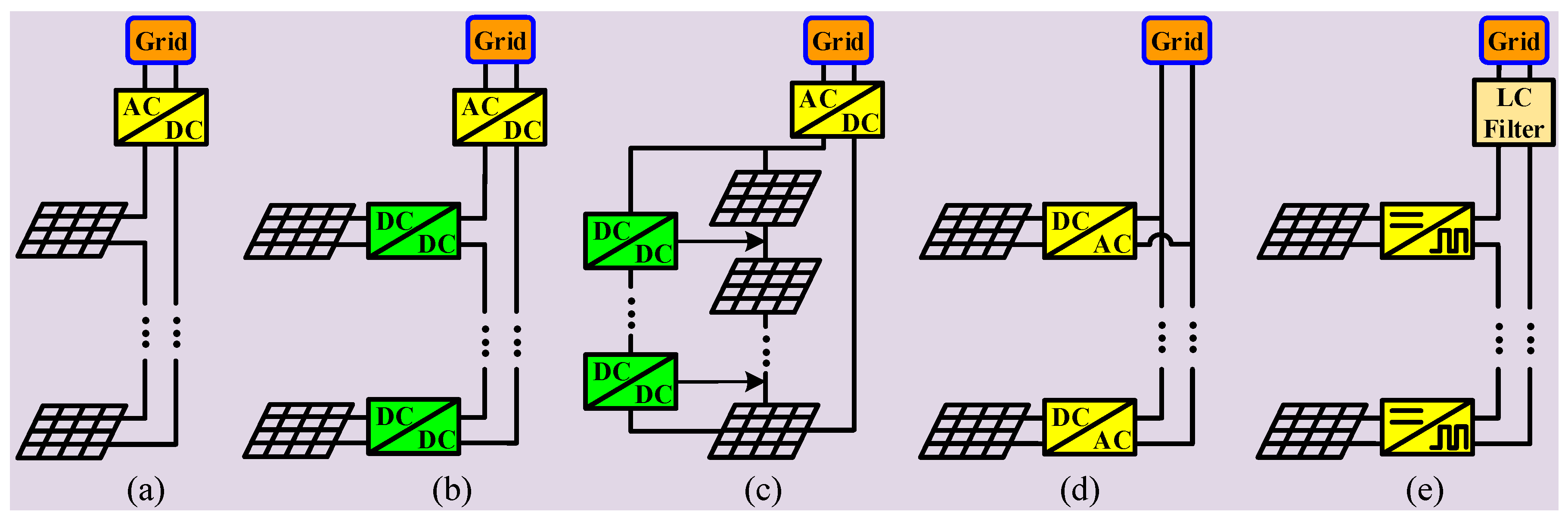
Over the past decades, many types of grid-connected PV generation architectures have been proposed. Among these PV generation configurations, the PV string centralized inverter architecture, cascaded DC/DC power optimizer architecture, differential power processing architecture, standard parallel inverter architecture and the multilevel cascaded H-Bridge architecture are five typical topologies (shown in Figure 1a–e, respectively) [7,8,9,10,11,12,13,14,15,16,17,18,19,20,21,22,23,24,25].
The PV string centralized inverter architecture, cascaded DC/DC power optimizer architecture and differential power processing architecture in Figure 1a–c all depend on a centralized interfacing inverter which interlinks with the grid. However, the limited power rating of the centralized inverter limits the capacity and scalability of the PV string. In Figure 1a, the output ports of the PV panels in the PV string centralized inverter architecture are connected in series and form a high DC-link voltage to match the grid voltage [8,9]. Then, the accumulated high DC voltage is inverted by a centralized inverter to achieve maximum power point tracking (MPPT) in the PV string. Since high voltage amplification is avoided, this system configuration has the advantages of high efficiency and low cost. For the cascaded DC/DC power optimizer architecture in Figure 1b, each PV panel is interfaced with a DC/DC power optimizer. Then, the output ports of these DC optimizers are connected in series to generate a higher DC voltage [10,11]. A high DC voltage gain in each DC/DC converter is not required and the distributed MPPT algorithm can be applied to the DC optimizers to achieve optimal energy capture of all PV panels. However, the reliability of maximum power extraction from each PV module is vulnerable when there is a mismatch between the distributed MPPT algorithm in the DC optimizers and the centralized MPPT algorithm in the centralized inverter [12,13,14]. Other than the cascaded DC/DC power optimizer architecture, the differential power processing architecture in Figure 1c is able to deal with the local mismatch to achieve local MPPT of each PV panel using low voltage (LV) power electronic devices [15,16]. So, differential power processing architecture suggests the potential to improve the efficiency and reliability.
Without the centralized interfacing inverter, the standard parallel inverter architecture shown in Figure 1d equips each PV panel with an independent interfacing inverter. The distributed MPPT algorithm is implemented in each parallel inverter to achieve maximum energy capture [17,18]. This topology exhibits the merits of high reliability, modularity for production and flexibility for plug and play. However, in order to match the grid voltage, a step-up transformer with high voltage gain is necessary for each PV module. So, relatively low efficiency and high cost are the drawbacks of this topology [19].
To improve the efficiency and lower the cost, the multilevel cascaded H-bridge architecture shown in Figure 1e promising PV generation configuration—has been investigated extensively [20,21,22,23,24,25]. Compared with standard parallel inverter architecture, the high frequency isolated transformer with high voltage gain is removed. An equivalent staircase output voltage is synthesized by the DC-link voltage of each PV module to match the grid voltage. Therefore, high system efficiency is achieved. Furthermore, this system configuration makes it much easier for LV PV modules to be integrated into the MV/HV grid. However, since all of the cascaded H-Bridge inverters are connected to the grid through a centralized LC filter, existing control methods for this topology are all dependent on the existence of centralized communication to coordinate the cascaded H-bridge inverters. Obviously, the reliance on centralized communication reduces the system’s reliability and increases the communication costs.
Recently, a series-connected microinverter-based grid-connected PV generation system was proposed [26]. In this set up, a high step-up power conditioning stage for each PV panel is not needed. In addition, each cascaded inverter has an independent output LC filter; thus, the output voltage of each inverter is controlled at the grid frequency, and all AC output voltages of these cascaded inverters are stacked up to match the grid voltage directly. Other than the multilevel cascaded H-bridge architecture, the system configuration in [26] facilitates the implementation of distributed control or even, fully decentralized control.
Based on the system configuration in [26], several communication-based control methods have been proposed [27,28,29,30,31]. In [27], a distributed autonomous control was first proposed. A fast output active power control loop and a slow voltage control loop were designed to achieve MPPT of all the PV modules simultaneously. However, this dynamic process and its reactive power regulation have not been discussed. Then, an improved distributed power control was proposed by [28] in which all cascaded inverters are controlled as voltage sources. With this distributed power control, the output active power and reactive power are regulated simultaneously to achieve MPPT of all the PV modules. On the other hand, refs. [29,30] proposed a hybrid current–voltage control scheme in which one of the cascaded PV inverters is controlled as a current source to regulate the line current, and other inverters are controlled as voltage sources to build up the voltage at the point of common coupling (PCC). In this way, the MPPT operations of all cascaded inverters are well ensured. However, the methods described in references [27,28,29,30] all require low-bandwidth communication links and phase-locked loops (PLL) to transfer the grid synchronization signal to each inverter. Different from references [27,28,29,30], reference [31] proposed a control method that equips each PV inverter string with a centralized controller to coordinate all cascaded inverters. In other words, centralized communication is required to make each inverter achieve an optimal power output. Obviously, the reliance of all cascaded inverters on low-bandwidth communication links [27,28,29,30,31] reduces the system’s reliability to a great extent due to the risk of case of communication failure. Moreover, the communication costs are high. In addition, the system modeling and stability proof of the proposed control methods in [27,28,29,30,31] were not derived.
According to the analysis above, no communication-free decentralized controls have been reported for the gird-connected cascaded PV inverter system. So, the starting point of this study was to design a fully communication-free decentralized control. In view of this, this paper proposes a communication-free decentralized control for the grid-connected cascaded PV inverter system, so as to improve the system’s reliability and reduce control complexity as well as communication costs. Similar to the system architecture in references [26,27,28,29,30,31], each cascaded inverter in the grid-connected cascaded PV inverter system has an independent output LC filter. A two-stage power conditioning stage with only low voltage gain is adopted, mainly to ensure a constant DC-link voltage for each cascaded inverter. The proposed communication-free decentralized control has two main contributions: (1) MPPT of all the cascaded PV converter units are achieved in a fully decentralized manner without any communication links; and (2) the frequency can self-synchronize with the grid and PLL is avoided. In this way, the system reliability is greatly improved compared with existing communication-dependent control methods Thus, communication costs are reduced. Small-signal modeling and eigenvalue analysis are conducted to evaluate the system’s stability under the proposed control and to help with the design of the system parameters. Simulation results are provided to verify the feasibility and effectiveness of the proposed control method.
The rest of this paper is organized as follows: In Section 2, the proposed system configuration is introduced, and power transfer characteristics are derived. In Section 3, the proposed communication-free decentralized control is elaborated. In Section 4, small-signal modeling and eigenvalue analysis are conducted. The simulation results are provided in Section 5. Conclusions are finally drawn in Section 6.
2. System Configuration and Power Transfer Characteristics
2.1. System Configuration
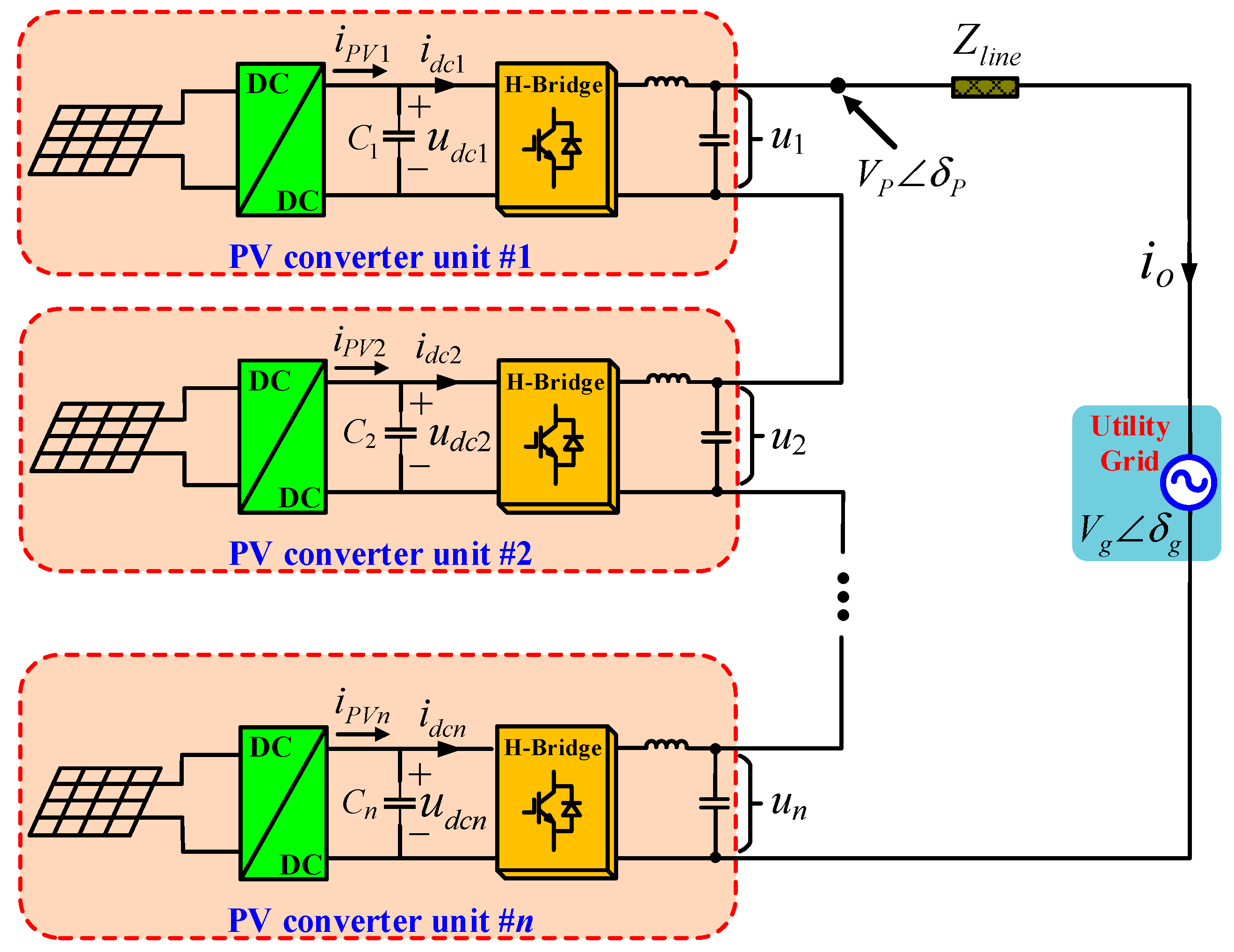
The configuration of the studied grid-connected cascaded PV inverter architecture with n PV inverter units is presented in Figure 2. Each PV converter unit contains a set of PV panels, a low-gain DC/DC converter, and a single phase full bridge inverter with an independent output LC filter. This configuration aims to supply the maximum power available to the utility grid from the solar energy captured by the PV panels.
Compared with other existing PV generation architectures, the grid-connected cascaded PV inverter system has obvious advantages, as follows:
- Interfacing inverters in the grid-connected cascaded PV inverter system are distributed but not centralized. Thus, the capacity limitation of the system caused by the centralized interfacing inverter is avoided. So, the scalability of this system configuration for MV/HV and the high-capacity PV grid-connection are enhanced;
- Each cascaded PV inverter has an independent output LC filter. The output voltage of each inverter is at grid frequency, indicating that distributed control and decentralized control are much easier to be realized. If so, system reliability can be improved significantly since centralized communication is avoided compared with multilevel cascaded H-bridge architecture;
- The output AC voltages of all the cascaded inverters are stacked up to match the grid voltage directly. This makes it much easier for LV PV generators to be integrated into the MV/HV grid since a high step-up transformer is avoided.
- On one hand, the step-up transformer is avoided compared with standard parallel inverter architecture. On the other hand, the studied cascaded PV inverter system enables a higher switching frequency and output LC filter components are thus shrunk [29,30]. So, losses are reduced, and higher efficiency is obtained [32].
- The low-gain two-stage power conditioning stage in each PV inverter unit can provide a constant DC-link voltage for each PV inverter;
- Each cascaded PV converter unit can be modularized for mass production.
2.2. Power Transfer Characteristics
According to Figure 2, the instantaneous output active power and reactive power of the i-th (i = 1,2,…,n) PV inverter, namely and , are calculated with
where Vi and δi denote the output voltage amplitude and phase of the i-th PV inverter. Vg and δg represent the grid voltage amplitude and phase angle. VP and δP are the voltage amplitude and phase angle at the point of common coupling (PCC). |Zline| and θline are the amplitude and phase angle of the line impedance, respectively. As is often the case, Zline is mainly inductive.
For this cascaded PV inverter architecture, the output voltages of all PV inverters sum up to
By substituting (3) into (1) and (2), the instantaneous output active power and reactive power of the i-th inverter are then rewritten as
3. Proposed Communication-Free Decentralized Control
3.1. Proposed Communication-Free Decentralized Control
In this section, a communication-free decentralized control strategy for the grid-connected cascaded PV inverter system is proposed. As all cascaded inverters share the same output current (io) in Figure 2, we only need to independently regulate the output active power of each inverter by controlling their output voltages. The proposed control is expressed as
where ωi, Vi, Pi, and ω* denote the output angular frequency reference, voltage amplitude reference, the average output active power of i-th PV converter unit and the rated grid angular frequency, respectively. udci and represent the real-time DC-link voltage and the DC voltage reference value of the i-th inverter, in which should be a constant larger than Vi to avoid over-modulation. mi is the frequency control coefficient. KPi and KIi stand for the proportional and integral coefficients of the DC-link voltage controller of the i-th inverter. V* is set equal to the rated grid voltage amplitude, V* = Vg. is the maximum active power reference of the i-th interfacing inverter, which is generated by the MPPT algorithm embedded in the front-end DC/DC stage.
3.2. Control Mechanism Analysis
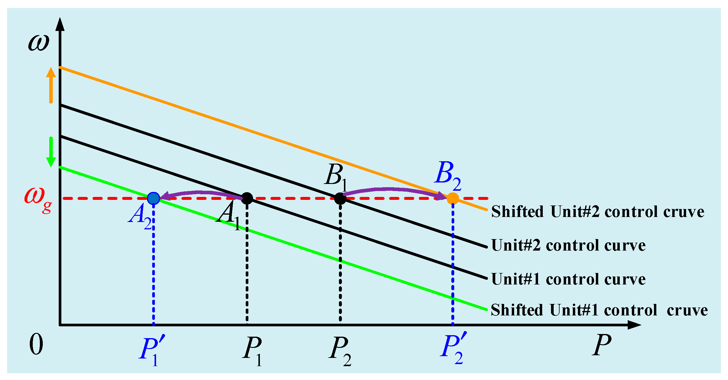
From (6), the output voltage amplitude reference of each inverter is the same, so the core idea of proposed control is regulating the angular frequency reference. The control expression (6) mainly contains two terms. The combination of the first term and the second term is designed to achieve MPPT and frequency self-synchronization. The second term is capable of regulating the DC-link voltage of each inverter. For better understanding of the proposed control, the control mechanism is properly illustrated in Figure 3.
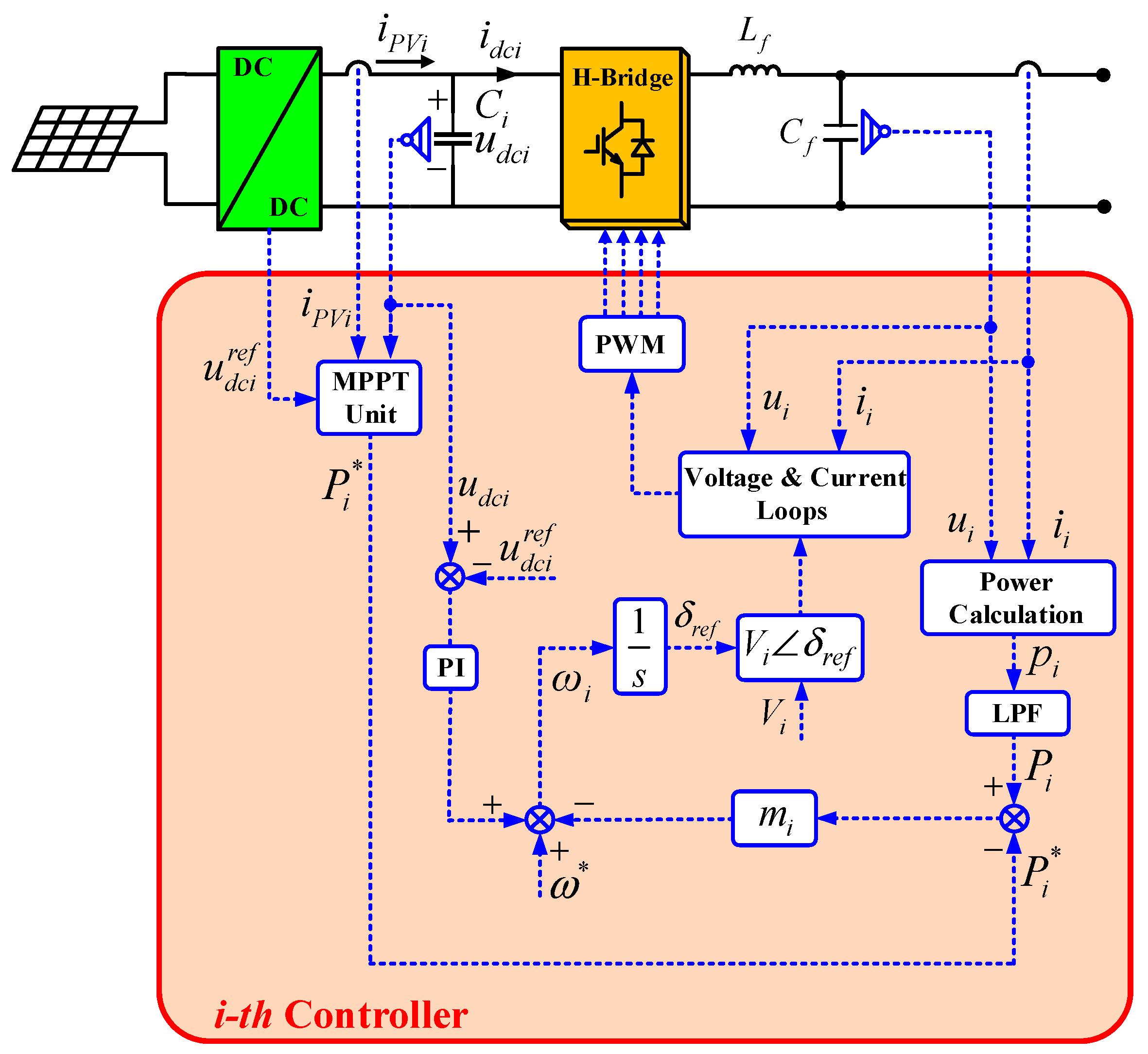
In Figure 3, a grid-connected cascaded PV inverter system consisting of only two cascaded PV converter units (unit#1 and unit#2) is presented to simplify the analysis, since a cascaded inverter system with more inverters has no significant technical differences. Firstly, from (4) and (5), the frequencies of all PV converter units must be identical and equal to grid frequency to reach a steady state. In Figure 3, the two PV converter units initially work at the steady-state operating points, A1 and B1, respectively. Their output frequencies are synchronous with the grid frequency, and their output active powers, P1 and P2, track their maximum active power references. The uncertainties of the weather, irradiance level, environmental temperature, and ageing of the PV panels should be taken into consideration. For instance, when the maximum active power available from unit#1 decreases from P1 to , its control curve is shifted down and its steady-state operating point moves from A1 to A2 accordingly. In this process, the steady-state operating point of unit#2 is not affected, and it keeps operating at its own maximum power point (MPP). Similarly, when the maximum active power available generated by unit#2 increases from P2 to , the control curve of unit#2 shifts up, and its steady-state operating point moves from B1 to B2. At the same time, the steady-state operating point of unit#1 is not affected, and it keeps operating at its MPP. Thus, all PV converter units in the cascaded system achieve MPPT operation independently and self-synchronize their frequencies with the grid. In other words, and are obtained at steady state. Moreover, with the second term in (6), the DC-link voltage of each PV converter unit can be regulated to its reference value at steady-state. A similar analysis process can be extended to other arbitrary operation conditions of unit#1 and unit#2 to properly explain the control mechanism. The completed control block diagram of the i-th cascaded PV inverter is presented in Figure 4.
From the analysis above, the proposed communication-free decentralized control has the following characteristics:
- No communication facilities are involved. All the controllers are fully decentralized. The output frequencies of all cascaded PV inverters self-synchronize with the grid frequency independently, with no need for PLL;
- MPPT operation of all the PV converter units is achieved simultaneously with only local output voltage control;
- A constant front-end DC-link voltage of each inverter is ensured.
4. Small-Signal Analysis
To study the system stability and dynamic performances of the proposed control strategy, a small-signal analysis was carried out. A small-signal model of the system in Figure 2 was first developed. Then, an eigenvalue analysis was conducted in order to evaluate the system’s stability and to reasonably design the system parameters to give satisfactory dynamic performances.
4.1. Small-Signal Modeling
First, denote the steady-state angular frequency as . To facilitate the small-signal modeling, we define and . In steady state, , so and hold. The angle of line impedance θline is a constant. By inserting (6) into (4), is rewritten as
Then, linearize (7) around the steady-state operating point:
where
Write (8) and (9) in matrix form:
where
From Figure 2, a mathematical model of the i-th inverter with the proposed control can be written as (11).
where udci and Ci are the DC-link voltage of the i-th inverter and the capacitor in DC side, respectively. represents the output PV current, as shown in Figure 2. The average output active power of the i-th inverter, Pi, is obtained by processing the instantaneous active power through a first-order low pass filter (LPF), and ωc is the cutoff frequency of the LPF. and are selected as state variables.
Then, we rewrite mathematical model (11) into (12):
By linearizing (12) around the steady-state operating point, the signal model of the i-th cascaded inverter is derived as
By substituting (8) into (13), (13) can be rewritten as
According to (14), the complete small-signal model of the cascaded PV inverter system in Figure 2 is obtained as
where
where Udci and represent the steady-state values of udci and , respectively.
So, the matrix form of the complete small-signal model of the system in Figure 2 can be obtained from (16):
where
In matrix A, and denote an n × n null matrix and an n × n identity matrix, respectively.
4.2. Eigenvalue Analysis
To evaluate the system’s stability and dynamic performance, an eigenvalue analysis of Jacobian matrix A in (16) was adopted. Based on the simulation model in Section 5 which consisted of 3 cascaded PV converter units, the system eigenvalues were analyzed while varying the control parameters: mi, KPi, KIi and DC-link capacitor Ci. The corresponding system parameters are presented in Table 1.
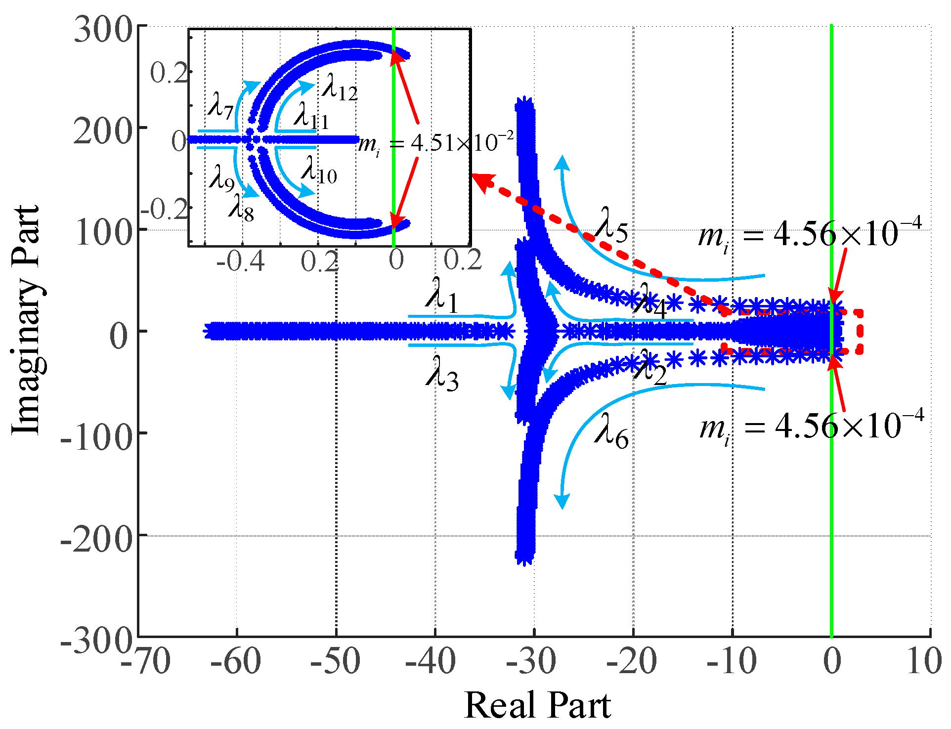
4.2.1. Frequency Control Coefficient (mi)
The system eigenvalue traces are shown for the variation of mi from 0 to 0.06, in Figure 5, in which and Ci = 8000 μF. In the beginning, when mi is small, there are two eigenvalues, λ5 and λ6, in the right-half plane, which means that the system is unstable. As mi increases, λ5 and λ6 move towards the left-half plane. When mi is larger than 4.56 × 10⁻⁴, all eigenvalues stay in the left-half plane, which indicates that the system has become stable. With a further increase in mi, λ1~λ6 move away from the imaginary axis. On the other hand, λ7~λ12 are dominant poles and move closer to the imaginary axis, which determines the system’s dynamic performance. When mi is larger than 4.51 × 10⁻², λ7 and λ10 reach the right-half plane, and the system becomes unstable. So, the stability range for mi is (4.56 × 10⁻⁴, 4.51 × 10⁻²). To ensure less oscillatory dynamics, small imaginary parts of the dominant poles, λ7~λ12, with a large damping ratio are required; therefore, mi = 0.005 is eventually selected.
4.2.2. DC-Link Voltage Controller Parameters (KPi and KIi)
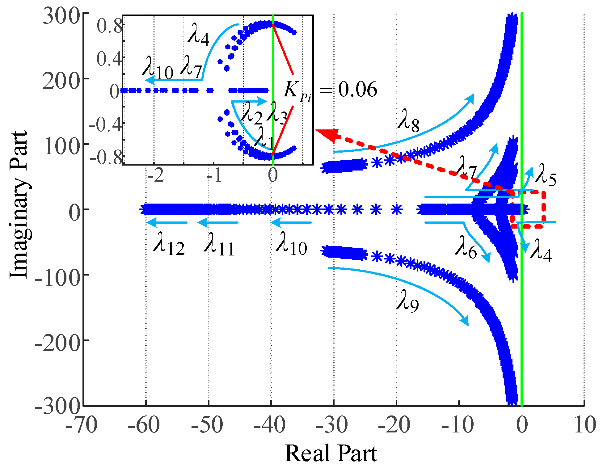
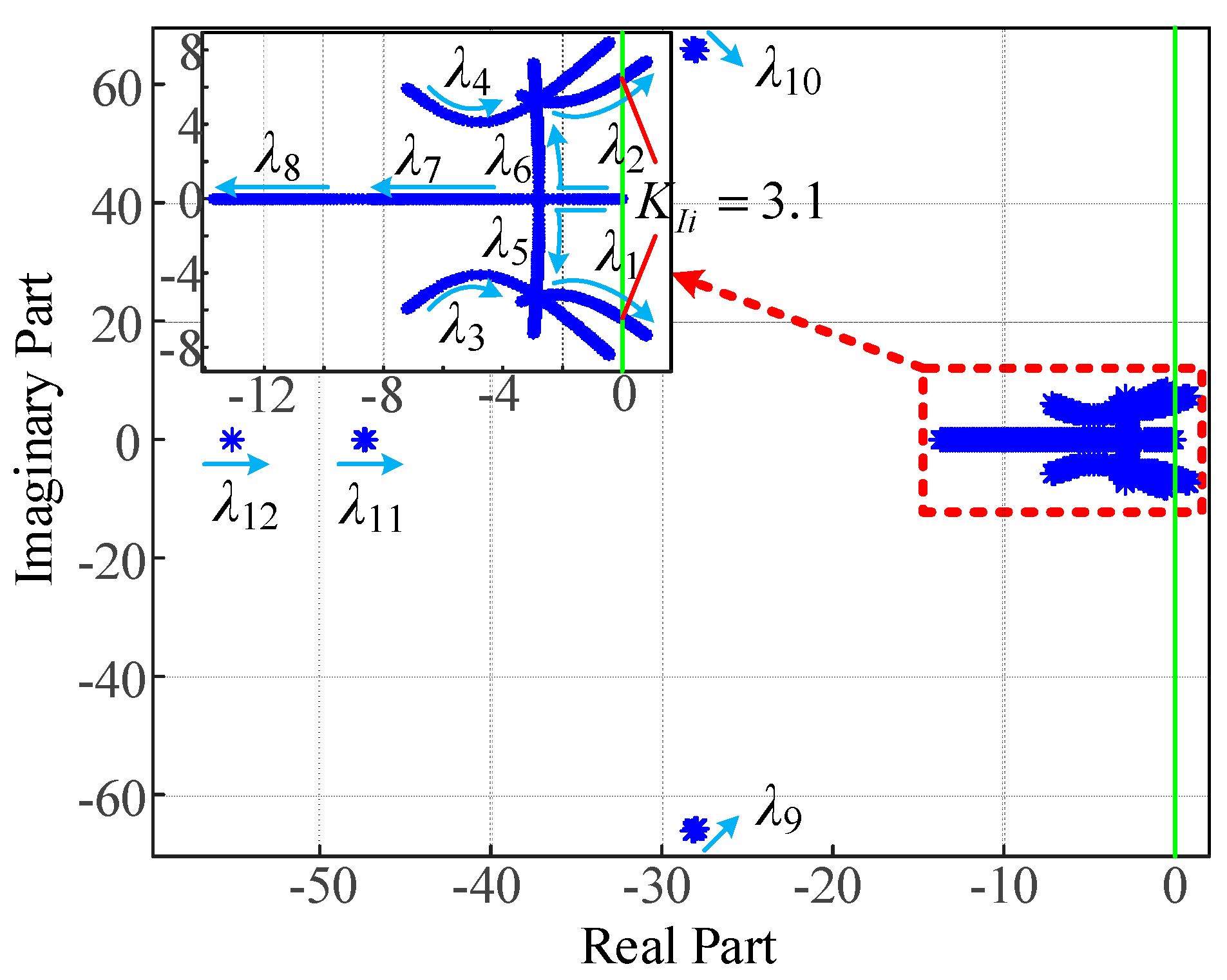
To better design the PI controller parameters, the system eigenvalue traces of varying KPi and KIi are sketched in Figure 6 and Figure 7 respectively, in which Ci = 8000 μF and mi = 5 × 10⁻³.
Figure 6 shows the eigenvalue traces for varying KPi from 0 to 50. In the beginning, when KPi is small, λ1~λ7 and λ10 are the dominant poles, and are much closer to the imaginary axis than λ8~λ9 and λ11~λ12. At the same time, λ1~λ4, λ7 and λ10 are in the right-half plane, which indicates that the system is unstable. When KPi increases to a value larger than 0.06, λ1~λ4, λ7 and λ10 reach the left-half plane, making the system stable. As KPi increases further, λ10 is positioned far away from the imaginary axis, while λ1~λ9 approach the imaginary axis but never reach it, which leads to a decreased system damping ratio. So, when KPi ϵ (0.06, 50), the system’s stability can be maintained.
Figure 7 shows the eigenvalue traces as KIi varies from 0 to 5. In the beginning, when KIi = 0, λ5~λ7 are at the origin while other eigenvalues are all in left-half plane, indicating that the system is critically stable. As KIi increases, all the eigenvalues stay in the left-half plane and system becomes stable. λ1~λ8 are the dominant poles and determine the system’s response speed. When KIi increases to 3.1, λ1 and λ2 move to the right-half plane; thus, the system becomes unstable. That is to say, the stability range for KIi is (0, 3.1).
To ensure the stability while making a tradeoff between stability and dynamic performance, relatively large, real parts of dominant poles and a large damping ratio are required. Thus, KPi = 0.5 and KIi = 0.05 were chosen.
4.2.3. DC-Side Capacitor (Ci)
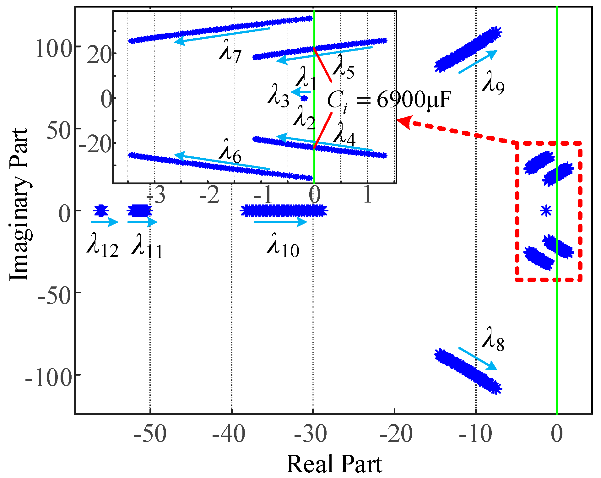
The system eigenvalue traces in which the capacitance value (Ci) is changed from 5000 μF to 10 mF are presented in Figure 8, where and mi = 5 × 10⁻³.
As shown in Figure 8, λ1~λ9 are the dominant poles, which determine the system’s dynamic response. Initially, when Ci is small, λ4 and λ5 lie in the unstable region. As Ci increases, λ4~λ7 move towards the left-half plane; meanwhile, the conjugate complex eigenvalues, λ4 and λ5, tend to move towards the imaginary axis. On the other hand, λ1~λ3 are almost unchanged—they are very close to the origin and almost not affected by the change in Ci. When Ci is larger than 6900 μF, λ4 and λ5 move to the left-half plane; thus, the system becomes stable. Hence, to ensure the stability of the system in this case, Ci should be larger than 6900 μF. In order to ensure the stability and high quality of the DC-link voltage, Ci = 8000 μF was used.
5. Simulation Results
This section describes simulation tests carried out in MATLAB/Simulink (2017a). Two simulation cases are presented. The first simulation case was conducted to verify the effectiveness and practicality of the proposed control in the utility grid-connected application. The second simulation case was designed to validate the scalability of the proposed control for the MV/HV grid-connected application.
5.1. Utility Grid-Connected Application
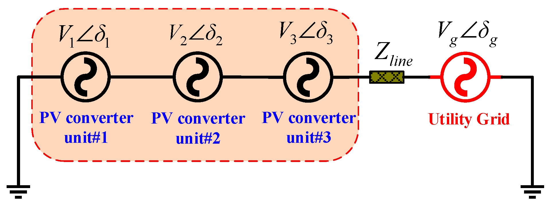
This simulation was based on a utility grid-connected cascaded PV inverter system with three PV converter units. The equivalent circuit of the simulation model is presented in Figure 9. The corresponding system parameters are listed in Table 1. The DC-link voltage reference of each inverter was set to 200 V to avoid over-modulation.
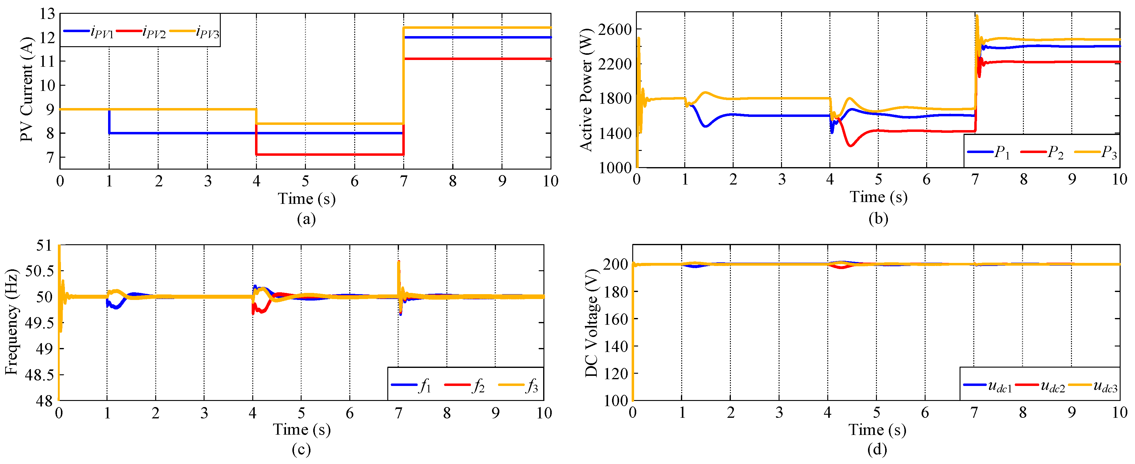
In this simulation test, a random change was imposed on the PV output current of each PV converter unit, so as to emulate the uncertainties of PV output caused by various factors. The PV output current of the cascaded PV converter units is presented in Figure 10a. The output active powers of the cascaded inverters are shown in Figure 10b. Figure 10c,d present the real-time output frequency and DC-link voltage of each cascaded inverter, respectively. The steady-state output voltages of the cascaded inverters and the corresponding line current under different operating conditions are shown in Figure 11.
As shown in Figure 10a, the PV output current of each PV converter unit changed randomly, which reflects the uncertainties in practical PV application occasions. Before t = 2 s, all of the PV output currents were the same (iPV1 = iPV2 = iPV3 = 9 A), as shown in Figure 10a. Thus, the maximum amounts of active power available were identical and the output active powers, P1, P2, P3, were the same at the steady state. When iPV1 suddenly dropped from 9 A to 8 A at t = 1 s (shown in Figure 10a), the maximum active power available for PV converter unit#1 decreased accordingly. As a result, P1 followed with an immediate decrease and eventually reached a new steady state. Furthermore, the steady-state values of P2 and P3 were not affected by the change in iPV1 because the values of iPV2 and iPV3 were still 9 A and the maximum active power available had not changed. At t = 4 s, iPV2 and iPV3 decreased to different values (iPV2 = 7.1 A, iPV3 = 8.4 A), while iPV1 remained unchanged, as shown in Figure 10a. Accordingly, P2 and P3 dropped to different values at steady state, tracking their maximum active power available. Additionally, the steady-state values of P1 were not affected and remained unchanged during this process. At t = 7 s, iPV1, iPV2 and iPV3 suddenly increased to different values simultaneously (iPV1 = 12 A; iPV2 = 11.1 A; iPV3 = 12.4 A), as shown in Figure 10a. At the same time, the output active powers, P1, P2 and P3, increased proportionally and finally, tracked their maximum active power reference precisely at steady state, as shown in Figure 10b. Therefore, we can see that the MPPT of all the PV converter units was achieved independently throughout the whole process with the proposed communication-free decentralized control. A shown in Figure 10c, frequency spikes occurred in the transient process because the output active power is regulated by controlling the phases of output voltages, which is consistent with the analysis in Section 3. Finally, all output frequencies of the cascaded inverters were able to converge to grid frequency at steady state (shown in Figure 10c), which indicates that the frequency self-synchronization with the utility grid was achieved simultaneously. Furthermore, Figure 10d shows that the DC-link voltages of all the cascaded inverters, udc1~udc3, were regulated to the reference values in steady state independently despite the random change in the PV output currents, iPV1, iPV2 and iPV3. So, a constant steady-state DC-link voltage was ensured for each inverter.
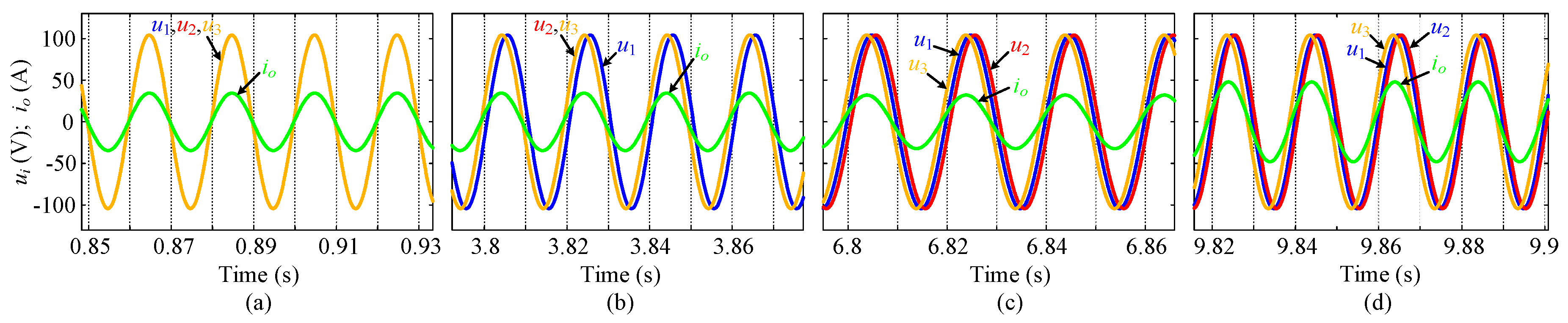
Steady-state output voltages and corresponding line current in different steady-state operating conditions are shown Figure 11. As shown in Figure 11a, the output voltage amplitudes and phase angles of all cascaded inverters were identical when iPV1 = iPV2 = iPV3. In Figure 11b, the voltage amplitudes of u1~u3 were still equal while the voltage phases of u2~u3 were a bit different from the voltage phase of u1 as a result of the difference between P2~P3 and P1. As shown in Figure 11c,d, the output voltage amplitudes of all inverters were still equal to their reference values while their phase angles were different during t = 4~10 s, because iPV1, iPV2 and iPV3 were different. So, a higher output active power is associated with a smaller phase angle difference with the line current. That is to say, the output active power of the cascaded inverters is regulated by controlling the output voltage phase angles, which is in accordance with the analysis in Section 3. Moreover, it is seen from Figure 11 that the line current amplitude was proportional to the total output active power of all inverters. In other words, a higher total active power injected to the grid is associated with a higher amplitude of the line current and vice versa.
5.2. Scalability for MV/HV Grid-Connected Application
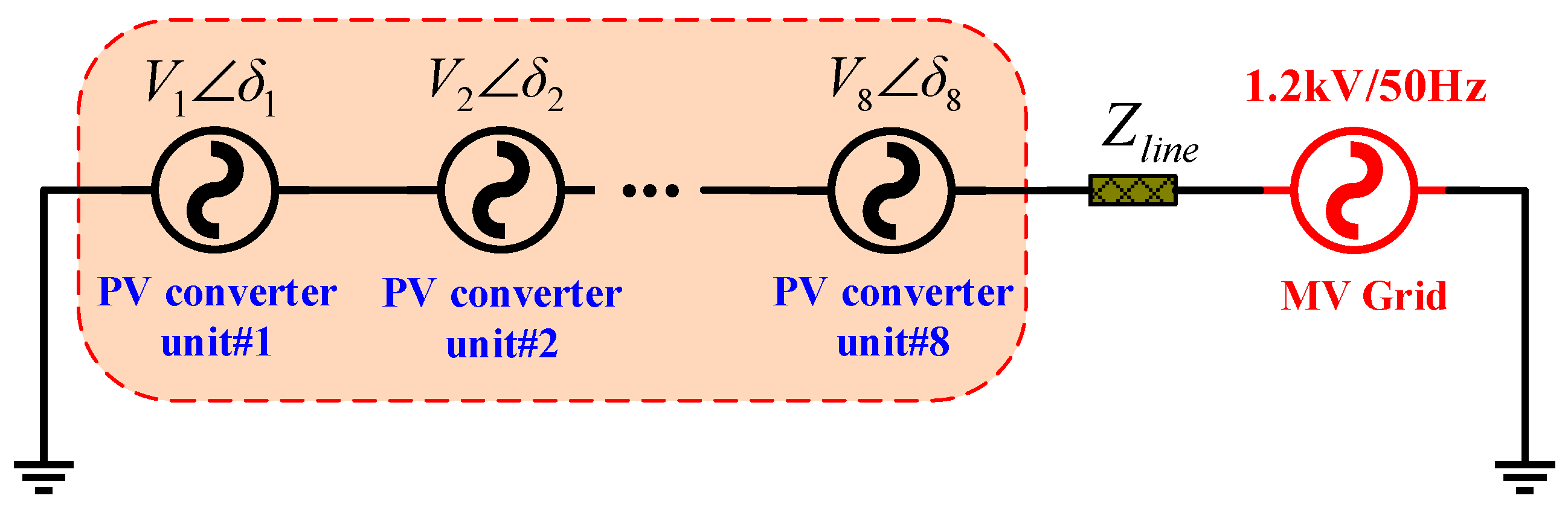
To demonstrate the scalability of the proposed control for the MV/HV grid-connected application, a simulation based on a MV grid-connected cascaded PV inverter system with eight PV converter units was conducted. For the HV grid-connection, a larger number of inverters is required due to the AC-stacked characteristics of the cascaded PV inverter system. In addition, a cascaded inverter system with more inverters has no technical differences. The voltage amplitude of the simulated MV grid was 1.2 kV. The output voltage amplitude of each inverter was 150 V. The other system parameters were same as those in Table 1. The equivalent circuit of this simulation model is shown in Figure 12.
The uncertainties of practical PV outputs were emulated by the use of random PV output current. As shown in Figure 13a, the PV output currents, iPV1~iPV3, were different, and iPV4~iPV8 were equal before t = 4 s (iPV1 = 6 A; iPV2 = 6.5 A; iPV3 = 7 A; iPV4 = iPV5 = … = iPV8 = 7.4 A). That is to say, the maximum amounts of active power available for PV converter unit#1 and PV converter unit#3 were different and the maximum amounts of active power available for PV converter unit#4 and PV converter unit#8 were identical. In Figure 13b, the output active powers, P1~P3, were different and P4~P8 were equal at steady-state where they were proportional to their PV output current and all PV inverters were operating at their MPPs. When iPV1~iPV8 suddenly increased simultaneously at t = 4 s (iPV1 = 10.1 A; iPV2 = 10.5 A; iPV3 = 11.1 A; iPV4 = iPV5 = … = iPV8 = 11.5 A) (shown in Figure 13a), the maximum active power available for all PV converter units increased accordingly (shown in Figure 13b). As a result, P1~P8 increased immediately, proportionally to their PV output currents and they still tracked their own maximum active power at a new steady state. As shown in Figure 13c, frequency spikes in the transient process occurred because that the output active power was regulated by controlling the phases of output voltages, which is consistent with the analysis in Section 3. The output frequencies of all cascaded inverters (f1~f8) were able to converge to grid frequency in steady state, which indicates that frequency self-synchronization with the utility grid was also achieved simultaneously. In Figure 13d, the DC-link voltages of all the cascaded inverters, udc1~udc8, were regulated independently by the reference values in steady state despite the random change in PV output currents, iPV1~iPV8. So, a constant steady-state DC-link voltage was ensured for each inverter.
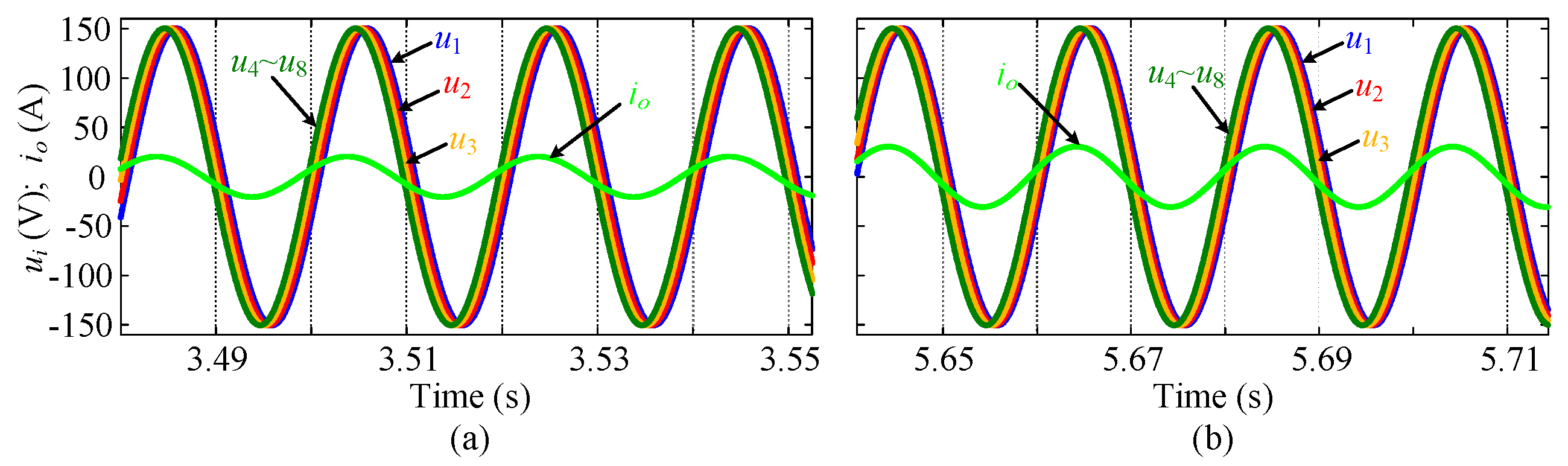
On the other hand, steady-state output voltages and corresponding line current in different steady-state operating conditions are shown Figure 14. As shown in Figure 14a,b the amplitudes of u1~u8 were identical. However, the phase angles of u1~u3 were a bit different while the phase angles of u4~u8 were equal, since a higher output active power means a smaller phase angle difference to the line current. So, we can see that the output active power of the cascaded inverters was regulated by controlling the output voltage phase angles, which is in accordance with the analysis in Section 3. Moreover, it is seen from Figure 14a,b that the steady-state amplitude of the line current after t = 4 s was larger than the steady-state amplitude before t = 4 s since the line current amplitude is proportional to the total output active power of all inverters.
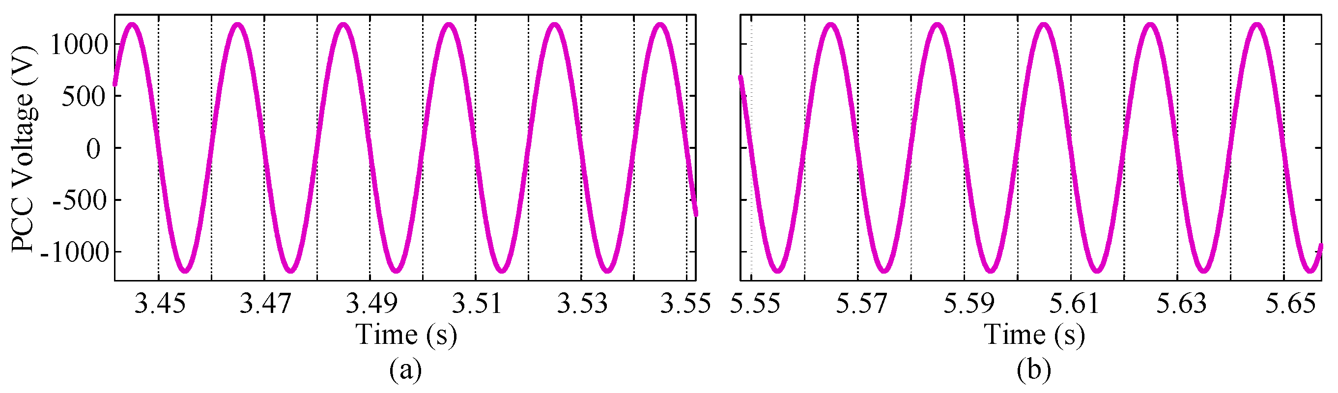
Moreover, the steady-state voltage at the PCC is shown in Figure 15. As shown in Figure 15a,b, the amplitude of the voltage at the PCC was similar to the grid voltage amplitude. Obviously, the cascaded PV inverter system can stack up the AC output voltages of all inverters to match the MV/HV grid directly with no need for high step-up transformer. So, the scalability of the cascaded PV inverter system and the proposed control in MV/HV grid-connected application were ensured.
6. Conclusions
Communication-free decentralized control of the grid-connected cascaded PV inverters was proposed in this paper. Compared with existing control methods, the proposed decentralized control involves no communication links. MPPT and frequency self-synchronization with the grid of all cascaded PV inverters are achieved locally. Thus, improved reliability, reduced control complexity and communication costs are obtained. The system’s stability and dynamic performance were evaluated by small-signal eigenvalue analysis. Finally, simulation results verified the feasibility and effectiveness of the proposed method.
The proposed communication-free decentralized control offers tremendous potential for cascaded PV inverters to be applied in large-scale MV/HV grid-connected PV generation, in which each PV inverter string contains numerous LV PV inverter units. In these applications, the proposed communication-free decentralized control would contribute to greatly improved system reliability and much reduced communication costs. Furthermore, this study also exhibits the possibility of inspiring potential communication-free solutions for hybrid-connection distributed generation networks, where cascaded inverters and parallel inverters are involved simultaneously.
Author Contributions
C.L. conceived the main idea and wrote the manuscript with guidance from X.H. and M.S. W.Y. and Z.L. performed the simulations; H.H. and J.M.G. reviewed the work and gave helpful improvement suggestions.
Acknowledgments
This work was supported by the National Natural Science Foundation of China under Grant 61573384 and Grant 51677195, and the Fundamental Research Funds for the Central Universities of Central South University under Grant 2018zzts531.
Conflicts of Interest
The authors declare no conflict of interest.
References
- Sun, Y.; Shi, G.; Li, X.; Yuan, W.; Su, M.; Han, H.; Hou, X. An f-P/Q Droop Control in Cascaded-Type Microgrid. IEEE Trans. Power Syst. 2018, 33, 1136–1138. [Google Scholar] [CrossRef]
- Han, H.; Li, L.; Wang, L.; Su, M.; Zhao, Y.; Guerrero, J.M. A Novel Decentralized Economic Operation in Islanded AC Microgrids. Energies 2017, 10, 804. [Google Scholar] [CrossRef]
- Hou, X.; Sun, Y.; Han, H.; Liu, Z.; Yuan, W.; Su, M. A fully decentralized control of grid-connected cascaded inverters. IEEE Trans. Power Del. 2018. [Google Scholar] [CrossRef]
- Meneses, D.; Blaabjerg, F.; García, Ó.; Cobos, J.A. Review and Comparison of Step-Up Transformerless Topologies for Photovoltaic AC-Module Application. IEEE Trans. Power Electron. 2013, 28, 2649–2663. [Google Scholar] [CrossRef]
- Liu, Z.; Su, M.; Sun, Y.; Han, H.; Hou, X.; Guerrero, J.M. Stability analysis of DC microgrids with constant power load under distributed control methods. Automatica 2018, 90, 62–72. [Google Scholar] [CrossRef]
- Kouro, S.; Leon, J.I.; Vinnikov, D.; Franquelo, L.G. Grid-Connected Photovoltaic Systems: An Overview of Recent Research and Emerging PV Converter Technology. IEEE Ind. Electron. Mag. 2015, 9, 47–61. [Google Scholar] [CrossRef]
- Li, Q.; Wolfs, P. A Review of the Single Phase Photovoltaic Module Integrated Converter Topologies with Three Different DC Link Configurations. IEEE Trans. Power Electron. 2008, 23, 1320–1333. [Google Scholar]
- Calais, M.; Myrzik, J.; Spooner, T.; Agelidis, V.G. Inverters for single-phase grid connected photovoltaic systems-an overview. In Proceedings of the 2002 IEEE 33rd Annual IEEE Power Electronics Specialists Conference, Cairns, Australia, 23–27 June 2002; pp. 1995–2000. [Google Scholar]
- Kjaer, S.B.; Pedersen, J.K.; Blaabjerg, F. A review of single-phase grid-connected inverters for photovoltaic modules. IEEE Trans. Ind. Appl. 2005, 41, 1292–1306. [Google Scholar] [CrossRef]
- Walker, G.R.; Sernia, P.C. Cascaded DC-DC converter connection of photovoltaic modules. IEEE Trans. Power Electron. 2004, 19, 1130–1139. [Google Scholar] [CrossRef]
- Bratcu, A.I.; Munteanu, I.; Bacha, S.; Picault, D.; Raison, B. Cascaded DC–DC Converter Photovoltaic Systems: Power Optimization Issues. IEEE Trans. Ind. Electron. 2011, 58, 403–411. [Google Scholar] [CrossRef]
- Linares, L.; Erickson, R.W.; MacAlpine, S.; Brandemuehl, M. Improved Energy Capture in Series String Photovoltaics via Smart Distributed Power Electronics. In Proceedings of the 2009 Twenty-Fourth Annual IEEE Applied Power Electronics Conference and Exposition, Washington, DC, USA, 15–19 February 2009; pp. 904–910. [Google Scholar]
- Alonso, R.; Roman, E.; Sanz, A.; Santos, V.E.M.; Ibanez, P. Analysis of Inverter-Voltage Influence on Distributed MPPT Architecture Performance. IEEE Trans. Ind. Electron. 2012, 59, 3900–3907. [Google Scholar] [CrossRef]
- Vitelli, M. On the necessity of joint adoption of both distributed maximum power point tracking and central maximum power point tracking in PV systems. Prog. Photovolt. Res. 2014, 22, 283–299. [Google Scholar] [CrossRef]
- Shenoy, P.S.; Kim, K.A.; Johnson, B.B.; Krein, P.T. Differential Power Processing for Increased Energy Production and Reliability of Photovoltaic Systems. IEEE Trans. Power Electron. 2013, 28, 2968–2979. [Google Scholar] [CrossRef]
- Kim, K.A.; Shenoy, P.S.; Krein, P.T. Converter Rating Analysis for Photovoltaic Differential Power Processing Systems. IEEE Trans. Power Electron. 2015, 30, 1987–1997. [Google Scholar] [CrossRef]
- Wills, R.H.; Krauthamer, S.; Bulawka, A.; Posbic, J.P. The AC photovoltaic module concept. In Proceedings of the Thirty-Second Intersociety Energy Conversion Engineering Conference (IECEC-97), Honolulu, HI, USA, 27 July–1 August 1997; Volume 3, pp. 1562–1563. [Google Scholar]
- Sun, Y.; Hou, X.; Yang, J.; Han, H.; Su, M.; Guerrero, J.M. New perspectives on droop control in AC microgrid. IEEE Trans. Ind. Electron. 2017, 64, 5741–5745. [Google Scholar] [CrossRef]
- Nanakos, A.C.; Tatakis, E.C.; Papanikolaou, N.P. A Weighted-Efficiency-Oriented Design Methodology of Flyback Inverter for AC Photovoltaic Modules. IEEE Trans. Power Electron. 2012, 27, 3221–3233. [Google Scholar] [CrossRef]
- Villanueva, E.; Correa, P.; Rodriguez, J.; Pacas, M. Control of a Single-Phase Cascaded H-Bridge Multilevel Inverter for Grid-Connected Photovoltaic Systems. IEEE Trans. Ind. Electron. 2009, 56, 4399–4406. [Google Scholar] [CrossRef]
- Malinowski, M.; Gopakumar, K.; Rodriguez, J.; Perez, M.A. A Survey on Cascaded Multilevel Inverters. IEEE Trans. Ind. Electron. 2010, 57, 2197–2206. [Google Scholar] [CrossRef]
- Liu, L.; Li, H.; Xue, Y.; Liu, W. Decoupled Active and Reactive Power Control for Large-Scale Grid-Connected Photovoltaic Systems Using Cascaded Modular Multilevel Converters. IEEE Trans. Power Electron. 2015, 30, 176–187. [Google Scholar]
- Liu, L.; Li, H.; Xue, Y.; Liu, W. Reactive Power Compensation and Optimization Strategy for Grid-Interactive Cascaded Photovoltaic Systems. IEEE Trans. Power Electron. 2015, 30, 188–202. [Google Scholar] [CrossRef]
- Xiao, M.; Xu, Q.; Ouyang, H. An Improved Modulation Strategy Combining Phase Shifted PWM and Phase Disposition PWM for Cascaded H-Bridge Inverters. Energies 2017, 10, 1327. [Google Scholar] [CrossRef]
- Tafti, H.D.; Maswood, A.I.; Konstantinou, G.; Townsend, C.D.; Acuna, P.; Pou, J. Flexible Control of Photovoltaic Grid-Connected Cascaded H-Bridge Converters During Unbalanced Voltage Sags. IEEE Trans. Ind. Electron. 2018, 65, 6229–6238. [Google Scholar] [CrossRef]
- Nuotio, M.; Ilic, M.; Liu, Y.; Bonanno, J.; Verlinden, P.J. Innovative AC photovoltaic module system using series connection and universal low-voltage micro inverters. In Proceedings of the 2014 IEEE 40th Photovoltaic Specialist Conference (PVSC), Denver, CO, USA, 8–13 June 2014; pp. 1367–1369. [Google Scholar]
- Lu, F.; Choi, B.; Maksimovic, D. Autonomous control of series-connected low voltage photovoltaic microinverters. In Proceedings of the 2015 IEEE 16th Workshop on Control and Modeling for Power Electronics (COMPEL), Vancouver, BC, Canada, 12–15 July 2015; pp. 1–6. [Google Scholar]
- Zhang, L.; Sun, K.; Li, Y.W.; Lu, X.; Zhao, J. A Distributed Power Control of Series-connected Module Integrated Inverters for PV Grid-tied Applications. IEEE Trans. Power Electron. 2017. [Google Scholar] [CrossRef]
- Jafarian, H.; Cox, R.; Enslin, J.H.; Bhowmik, S.; Parkhideh, B. Decentralized Active and Reactive Power Control for an AC-Stacked PV Inverter with Single Member Phase Compensation. IEEE Trans. Ind. Appl. 2018, 54, 345–355. [Google Scholar] [CrossRef]
- Jafarian, H.; Bhowmik, S.; Parkhideh, B. Hybrid Current-/Voltage-Mode Control Scheme for Distributed AC-Stacked PV Inverter with Low-Bandwidth Communication Requirements. IEEE Trans. Ind. Electron. 2018, 65, 321–330. [Google Scholar] [CrossRef]
- He, J.; Li, Y.; Wang, C.; Pan, Y.; Zhang, C.; Xing, X. Hybrid Microgrid With Parallel- and Series-Connected Microconverters. IEEE Trans. Power Electron. 2018, 33, 4817–4831. [Google Scholar] [CrossRef]
- Bhowmik, S. Systems and Methods for Solar Photovoltaic Energy Collection and Conversion. U.S. Patent 9531293 B2, 27 December 2016. [Google Scholar]
Figure 1.
Five typical photovoltaic (PV) generation topologies. (a) PV string centralized inverter architecture. (b) Cascaded DC/DC power optimizer architecture. (c) Differential power processing architecture. (d) Standard parallel inverter architecture. (e) Multilevel cascaded H-Bridge architecture.

Figure 2.
Configuration of the grid-connected cascaded PV inverter system.

Figure 3.
Control mechanism of frequency self-synchronization and maximum power point tracking (MPPT).
Figure 3.
Control mechanism of frequency self-synchronization and maximum power point tracking (MPPT).

Figure 4.
Control block diagram of the i-th cascaded PV inverter.

Figure 5.
Eigenvalue traces of varying the frequency control coefficient, mi ().

Figure 6.
Eigenvalue traces of varying KPi in ().

Figure 7.
Eigenvalue traces of varying KIi (the integral coefficient of the DC-link voltage controller of the i-th inverter) in ().
Figure 7.
Eigenvalue traces of varying KIi (the integral coefficient of the DC-link voltage controller of the i-th inverter) in ().

Figure 8.
Eigenvalue traces of varying the DC-side capacitor (Ci) in ().

Figure 9.
Equivalent circuit of the utility grid-connection simulation model.

Figure 10.
(a) PV output current. (b) Output active power. (c) Output frequency. (d) DC-link voltages of the cascaded inverters.
Figure 10.
(a) PV output current. (b) Output active power. (c) Output frequency. (d) DC-link voltages of the cascaded inverters.

Figure 11.
Steady-state line current and output voltages of the cascaded inverters under different operating conditions: (a) iPV1 = iPV2 = iPV2 = 9 A. (b) iPV1 = 8 A; iPV2 = iPV3 = 9 A. (c) iPV1 = 8 A; iPV2 = 7.1 A; iPV3 = 8.4 A. (d) iPV1 = 12 A; iPV2 = 11.1 A; iPV3 = 12.4 A.
Figure 11.
Steady-state line current and output voltages of the cascaded inverters under different operating conditions: (a) iPV1 = iPV2 = iPV2 = 9 A. (b) iPV1 = 8 A; iPV2 = iPV3 = 9 A. (c) iPV1 = 8 A; iPV2 = 7.1 A; iPV3 = 8.4 A. (d) iPV1 = 12 A; iPV2 = 11.1 A; iPV3 = 12.4 A.

Figure 12.
Equivalent circuit of the medium voltage (MV) grid-connection simulation model.

Figure 13.
(a) PV output current. (b) Output active power. (c) Output frequency. (d) DC-link voltages of the cascaded inverters.
Figure 13.
(a) PV output current. (b) Output active power. (c) Output frequency. (d) DC-link voltages of the cascaded inverters.

Figure 14.
Steady-state line current and output voltages of the cascaded inverters under different operating conditions. (a) iPV1 = 6 A; iPV2 = 6.5 A; iPV3 = 7 A; iPV4 = iPV5 = … = iPV8 = 7.4 A. (b) iPV1 = 10.1 A; iPV2 = 10.5 A; iPV3 = 11.1 A; iPV4 = iPV5 = … = iPV8 = 11.5 A.
Figure 14.
Steady-state line current and output voltages of the cascaded inverters under different operating conditions. (a) iPV1 = 6 A; iPV2 = 6.5 A; iPV3 = 7 A; iPV4 = iPV5 = … = iPV8 = 7.4 A. (b) iPV1 = 10.1 A; iPV2 = 10.5 A; iPV3 = 11.1 A; iPV4 = iPV5 = … = iPV8 = 11.5 A.

Figure 15.
Steady-state voltage at the PCC. (a) iPV1 = 6 A; iPV2 = 6.5 A; iPV3 = 7 A; iPV4 = iPV5 = … = iPV8 = 7.4 A. (b) iPV1 = 10.1 A; iPV2 = 10.5 A; iPV3 = 11.1 A; iPV4 = iPV5 = … = iPV8 = 11.5 A.
Figure 15.
Steady-state voltage at the PCC. (a) iPV1 = 6 A; iPV2 = 6.5 A; iPV3 = 7 A; iPV4 = iPV5 = … = iPV8 = 7.4 A. (b) iPV1 = 10.1 A; iPV2 = 10.5 A; iPV3 = 11.1 A; iPV4 = iPV5 = … = iPV8 = 11.5 A.


Table 1.
Simulation parameters.
| Item | Symbol | Value |
|---|---|---|
| Grid voltage | Vg/fg | 311 V/50 Hz |
| Voltage amplitude reference | V1 = V2 = V3 | 311/3 V |
| Droop coefficients | m1 = m2 = m3 | 5 × 10⁻³ |
| Proportional coefficients | KP1 = KP2 = KP3 | 0.5 |
| Integral coefficients | KI1 = KI2 = KI3 | 0.05 |
| Capacitor in DC-side | C1 = C2 = C3 | 8000 μF |
| DC voltage reference | = = | 200 V |
| Line impedance | Zline | 0.1 + j0.94 Ω |
| Rated angular frequency | ω* | 100π rad/s |
© 2018 by the authors. Licensee MDPI, Basel, Switzerland. This article is an open access article distributed under the terms and conditions of the Creative Commons Attribution (CC BY) license (http://creativecommons.org/licenses/by/4.0/).
Share and Cite
MDPI and ACS Style
Su, M.; Luo, C.; Hou, X.; Yuan, W.; Liu, Z.; Han, H.; Guerrero, J.M. A Communication-Free Decentralized Control for Grid-Connected Cascaded PV Inverters. Energies 2018, 11, 1375. https://doi.org/10.3390/en11061375
AMA Style
Su M, Luo C, Hou X, Yuan W, Liu Z, Han H, Guerrero JM. A Communication-Free Decentralized Control for Grid-Connected Cascaded PV Inverters. Energies. 2018; 11(6):1375. https://doi.org/10.3390/en11061375
Chicago/Turabian StyleSu, Mei, Chao Luo, Xiaochao Hou, Wenbin Yuan, Zhangjie Liu, Hua Han, and Josep M. Guerrero. 2018. "A Communication-Free Decentralized Control for Grid-Connected Cascaded PV Inverters" Energies 11, no. 6: 1375. https://doi.org/10.3390/en11061375
Note that from the first issue of 2016, this journal uses article numbers instead of page numbers. See further details here.