Multiple Fuel Machines Power Economic Dispatch Using Stud Differential Evolution

 , , , ,
Abstract
:1. Introduction
2. Problem Formulation
2.1. Objective Function
2.2. Constraints
2.2.1. Equality Constraint
2.2.2. In-Equality Constraint
2.3. Fuel Cost Equations
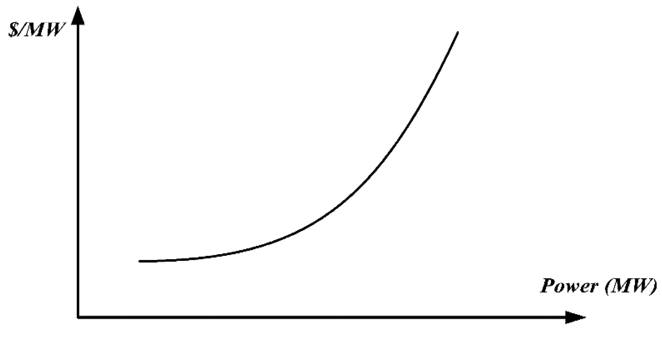
2.3.1. Power Economic Dispatch considering Valve Point Loading Effects Only
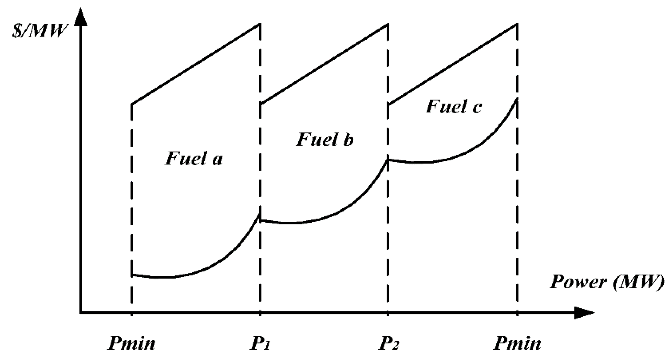
2.3.2. Power Economic Dispatch Considering Multiple Fuel Options Only
2.3.3. Power Economic Dispatch Considering Multiple Fuel Options and Valve Point Loading Effects Together
3. Differential Evolution (DE)
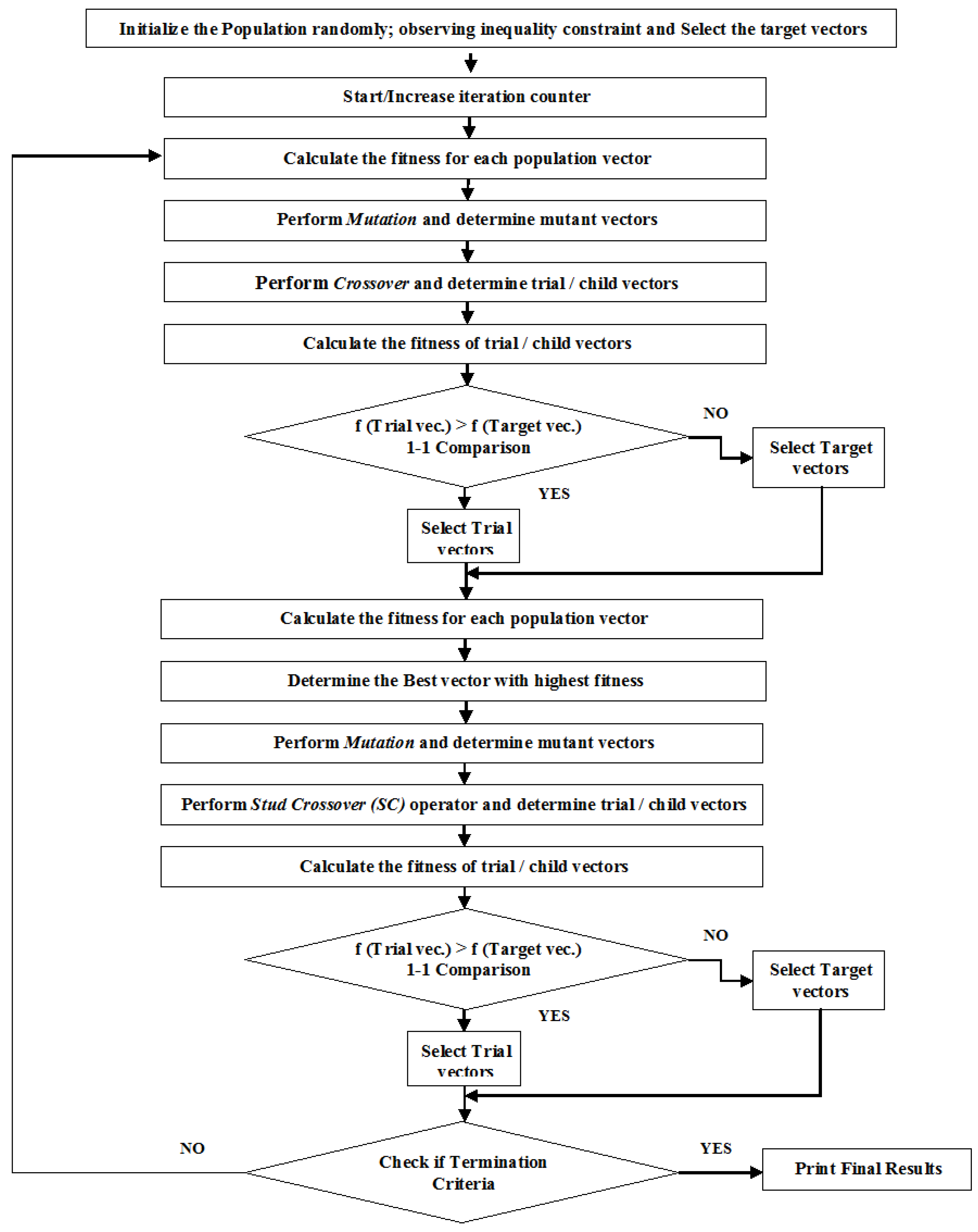
4. Stud Differential Evolution (SDE)
| Algorithm 1: Stud Differential Evolution (SDE) |
| Begin Randomly initialize the population P (target vectors) of NP size and of D dimensions, in a feasible range Set the generation counter G = 1 Allot suitable values to all other control parameters i.e., crossover rate CR, mutation probability F etc. Calculate the fitness for all generated population vectors. While G < Maximum Generation do Implement regular DE from conventional mutational and crossover all the way to selection. for I = 1: NP do Perform Mutation and generate mutant vector Perform the SC operator in Algorithm 2 end for i Sort all the vectors and find the current best vector G = G + 1; end while Display the best solution. End. |
| Algorithm 2: Stud Crossover (SC) Operator |
| Begin Perform the Selection Select the Stud/Best vector for mating Perform the Crossover Generate trial vector , taking stud as first parent and mutant vector as a second parent Calculate fitness of trial vector () If () do Accept the generated trial vector for next generationelse else Accept the generated target vector for next generation end if End. |
5. Simulation Results
5.1. System 1: 10 Machine Multiple Fuel Convex PED (without Valve Point Loading Effects)
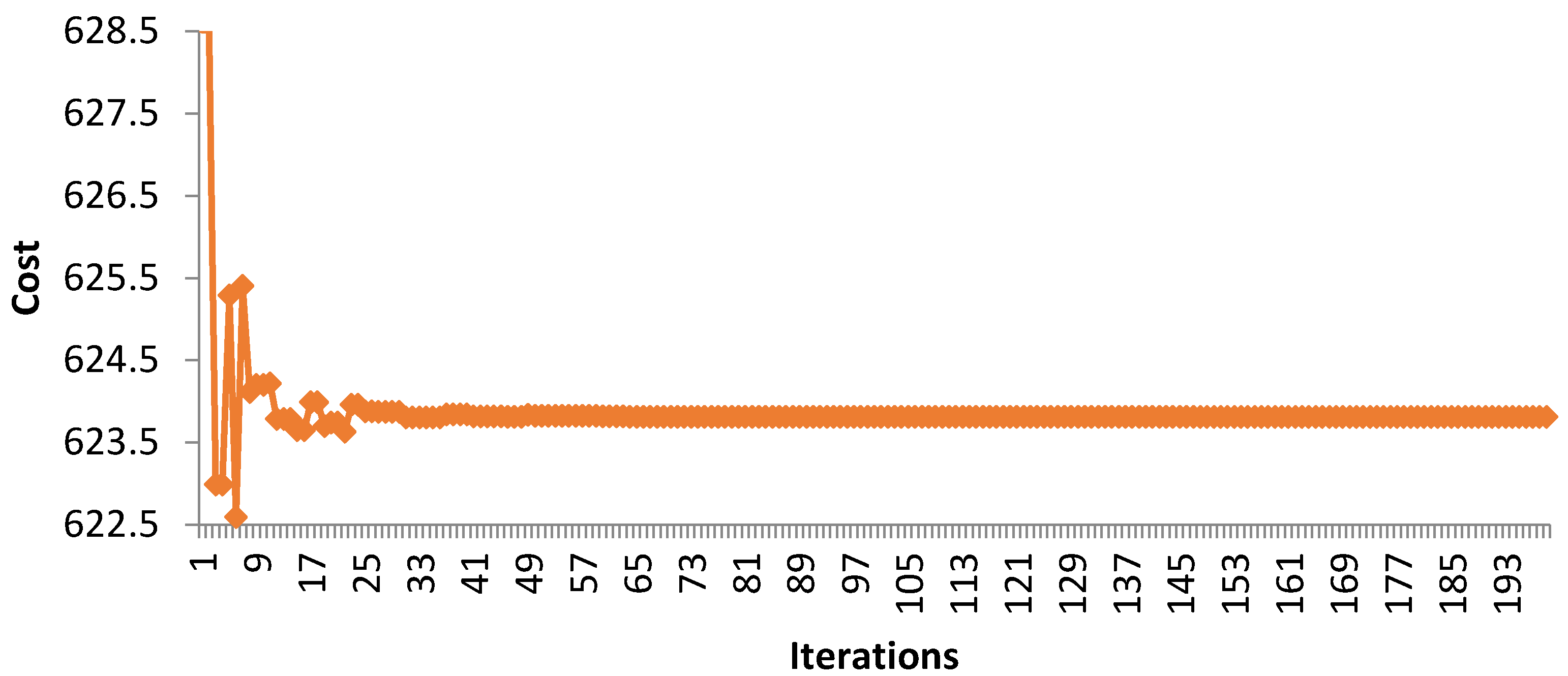
5.2. System 2: 10 Machine Multiple Fuel Non-Convex PED (with Valve Point Loading Effects)
6. Conclusions
- SDE is a potential solution methodology for the PED problem, as it addresses the convex and non-convex PED equally.
- Results obtained from SDE are better in comparison with the current research available, which indicates the promise of the approach.
- SDE can easily be further modified and hybridized with other optimization techniques because it has fewer control parameters.
Author Contributions
Acknowledgments
Conflicts of Interest
Nomenclature
| Total no. of units | |
| Power from ith unit | |
| Fuel cost associated with ith unit | |
| Total power demand | |
| Minimum power generation from ith unit | |
| Maximum power generation from ith unit | |
| Minimum power generation from ith unit consuming kth fuel | |
| Maximum power generation from ith unit consuming kth fuel | |
| Total cost of power generation | |
| , | Cost coefficients of the ith generating unit consuming kth fuel |
| Optimization Techniques | |
| AIS | Artificial Immune System |
| APSO | Adaptive particle swarm optimization |
| ASA | Adaptive Simulated Annealing |
| BSA | Back-tracking Search Algorithm |
| CBPSO_RVM | Combined particle swarm optimization with real-valued mutation |
| CGA_MU | Conventional Genetic Algorithm with Multiplier Updating |
| C-GRASP–DE | Continuous Greedy Randomized Adaptive Search Procedure with Differential Evolution |
| CPSO | Combinatorial particle swarm optimization |
| CSA-Cauchy | Cuckoo Search Algorithm with Cauchy distribution |
| CSA-Gauss | Cuckoo Search Algorithm with Gaussian distribution |
| DEPSO | Differential Evolution with Particle Swarm Optimization |
| DSPSO_TSA | Distributed Sobol Particle Swarm Optimization and Tabu Search Algorithm |
| EALHN | Enhanced Augmented Lagrange Hopfield Network |
| GA_BGC | Genetic Algorithm with best of Gaussian and Cauchy mutations |
| GA_C | Genetic Algorithm GA with Cauchy mutation |
| GA_G | Genetic Algorithm with Gaussian mutation |
| GA_MGC | Genetic Algorithm with mean of Gaussian and Cauchy mutations |
| GHS | Global-best Harmony Search |
| HLN | Hopfield Lagrange Network |
| HNN | Hopfiled Neural Network |
| IDE | Improved Differential Evolution |
| IEP | Improved Evolutionary Programming |
| IGA_MU | Improved Genetic Algorithm with Multiplier Updating |
| IODPSO_G | improved orthogonal design particle swarm optimization with global star structure |
| IODPSO_L | improved orthogonal design particle swarm optimization with local ring structure |
| LI | Lamda-iteration |
| MHNN | Modified Hopfield Neural Network |
| MPSO | Modified Particle Swarm Optimization |
| MSFLA | Modified Shuffled Frog Leaping Algorithm |
| NPSO | New particle swarm optimization |
| QPSO | Quantum-behaved particle swarm optimization |
| RCGA | Real-coded Genetic Algorithm |
| SADE_ALM | Self-adaptive Differential Evolution method with Augmented Lagrange Multiplier |
| SDE | Stud Differential Evolution |
| SFLA-GHS | shuffled frog leaping algorithm with global-best harmony search algorithm |
References
- Sayah, S.; Hamouda, A. A new hybrid heuristic algorithm for the nonconvex economic dispatch problem. In Proceedings of the 2017 5th International Conference on Electrical Engineering-Boumerdes (ICEE-B), Boumerdes, Algeria, 29–31 October 2017; pp. 1–6. [Google Scholar]
- Wood, A.J.; Wollenberg, B.F. Power Generation, Operation, and Control; John Wiley & Sons: Hoboken, NJ, USA, 2012. [Google Scholar]
- Hindi, K.S.; Ab Ghani, M. Dynamic economic dispatch for large scale power systems: A lagrangian relaxation approach. Int. J. Electr. Power Energy Syst. 1991, 13, 51–56. [Google Scholar] [CrossRef]
- Liang, Z.-X.; Glover, J.D. A zoom feature for a dynamic programming solution to economic dispatch including transmission losses. IEEE Trans. Power Syst. 1992, 7, 544–550. [Google Scholar] [CrossRef]
- Papageorgiou, L.G.; Fraga, E.S. A mixed integer quadratic programming formulation for the economic dispatch of generators with prohibited operating zones. Electr. Power Syst. Res. 2007, 77, 1292–1296. [Google Scholar] [CrossRef]
- Victoire, T.A.A.; Jeyakumar, A.E. Deterministically guided pso for dynamic dispatch considering valve-point effect. Electr. Power Syst. Res. 2005, 73, 313–322. [Google Scholar] [CrossRef]
- Khamsawang, S.; Jiriwibhakorn, S. Dspso–tsa for economic dispatch problem with nonsmooth and noncontinuous cost functions. Energy Convers. Manag. 2010, 51, 365–375. [Google Scholar] [CrossRef]
- Ab Ghani, M.R.; Hussein, S.T.; Ruddin, M.; Mohamad, M.; Jano, Z. An examination of economic dispatch using particle swarm optimization. MAGNT Res. Rep. 2015, 3, 193–209. [Google Scholar]
- Duman, S.; Yorukeren, N.; Altas, I.H. A novel modified hybrid psogsa based on fuzzy logic for non-convex economic dispatch problem with valve-point effect. Int. J. Electr. Power Energy Syst. 2015, 64, 121–135. [Google Scholar] [CrossRef]
- Júnior, J.d.A.B.; Nunes, M.V.A.; Nascimento, M.H.R.; Rodríguez, J.L.M.; Leite, J.C. Solution to economic emission load dispatch by simulated annealing: Case study. Electr. Eng. 2017, 1–13. [Google Scholar] [CrossRef]
- Lin, W.-M.; Cheng, F.-S.; Tsay, M.-T. An improved tabu search for economic dispatch with multiple minima. IEEE Trans. Power Syst. 2002, 17, 108–112. [Google Scholar] [CrossRef]
- Aydin, D.; Yavuz, G.; Özyön, S.; Yaşar, C.; Stützle, T. Artificial Bee colony framework to non-convex economic dispatch problem with valve point effects: A case study. In Proceedings of the Genetic and Evolutionary Computation Conference Companion, Berlin, Germany, 15–19 July 2017; pp. 1311–1318. [Google Scholar]
- Mouassa, S.; Bouktir, T. Artificial bee colony algorithm for solving economic dispatch problems with non-convex cost functions. Int. J. Power Energy Convers. 2017, 8, 146–165. [Google Scholar] [CrossRef]
- Karthik, N.; Parvathy, A.; Arul, R. Non-convex economic load dispatch using cuckoo search algorithm. Indones. J. Electr. Eng. Comput. Sci. 2017, 5, 48–57. [Google Scholar] [CrossRef]
- Souza, R.O.G.; Oliveira, E.S.; Junior, I.C.S.; Marcato, A.L.M.; de Olveira, M.T. Flower pollination algorithm applied to the economic dispatch problem with multiple fuels and valve point effect. In Proceedings of the Portuguese Conference on Artificial Intelligence, Porto, Portugal, 5–8 September 2017; pp. 260–270. [Google Scholar]
- Bhattacharya, S.; Kuanr, B.R.; Routray, A.; Dash, A. Implementation of bat algorithm in economic dispatch for units with multiple fuels and valve-point effect, Electrical. In Proceedings of the 2017 IEEE International Conference on Instrumentation and Communication Engineering (ICEICE), Karur, India, 27–28 April 2017; pp. 1–7. [Google Scholar]
- Kheshti, M.; Kang, X.; Bie, Z.; Jiao, Z.; Wang, X. An effective lightning flash algorithm solution to large scale non-convex economic dispatch with valve-point and multiple fuel options on generation units. Energy 2017, 129, 1–15. [Google Scholar] [CrossRef]
- Kamboj, V.K.; Bhadoria, A.; Bath, S. Solution of non-convex economic load dispatch problem for small-scale power systems using ant lion optimizer. Neural Comput. Appl. 2017, 28, 2181–2192. [Google Scholar] [CrossRef]
- Cui, S.; Wang, Y.-W.; Lin, X.; Liu, X.-K. Distributed auction optimization algorithm for the nonconvex economic dispatch problem based on the gossip communication mechanism. Int. J. Electr. Power Energy Syst. 2018, 95, 417–426. [Google Scholar] [CrossRef]
- Bentouati, B.; Chaib, L.; Chettih, S.; Wang, G.-G. An efficient stud krill herd framework for solving non-convex economic dispatch problem. World Acad. Sci. Eng. Technol. Int. J. Electr. Comput. Energ. Electron. Commun. Eng. 2017, 11, 1095–1100. [Google Scholar]
- Das, D.; Bhattacharya, A.; Ray, R. Symbiotic organisms search algorithm for economic dispatch problems. In Proceedings of the 2017 Second International Conference on Electrical, Computer and Communication Technologies (ICECCT), Coimbatore, India, 22–24 February 2017; pp. 1–7. [Google Scholar]
- Dihem, A.; Salhi, A.; Naimi, D.; Bensalem, A. Solving smooth and non-smooth economic dispatch using water cycle algorithm. In Proceedings of the 2017 5th International Conference on Electrical Engineering-Boumerdes (ICEE-B), Boumerdes, Algeria, 29–31 October 2017; pp. 1–6. [Google Scholar]
- Pham, L.H.; Nguyen, T.T.; Vo, D.N.; Tran, C.D. Adaptive cuckoo search algorithm based method for economic load dispatch with multiple fuel options and valve point effect. Int. J. Hybrid Inf. Technol. 2016, 9, 41–50. [Google Scholar] [CrossRef]
- Lee, S.-C.; Kim, Y.-H. An enhanced lagrangian neural network for the eld problems with piecewise quadratic cost functions and nonlinear constraints. Electr. Power Syst. Res. 2002, 60, 167–177. [Google Scholar] [CrossRef]
- Secui, D.C. A modified symbiotic organisms search algorithm for large scale economic dispatch problem with valve-point effects. Energy 2016, 113, 366–384. [Google Scholar] [CrossRef]
- Adarsh, B.; Raghunathan, T.; Jayabarathi, T.; Yang, X.-S. Economic dispatch using chaotic bat algorithm. Energy 2016, 96, 666–675. [Google Scholar] [CrossRef]
- Selvakumar, A.I.; Thanushkodi, K. A new particle swarm optimization solution to nonconvex economic dispatch problems. IEEE Trans. Power Syst. 2007, 22, 42–51. [Google Scholar] [CrossRef]
- Chiang, C.-L. Improved genetic algorithm for power economic dispatch of units with valve-point effects and multiple fuels. IEEE Trans. Power Syst. 2005, 20, 1690–1699. [Google Scholar] [CrossRef]
- Lu, H.; Sriyanyong, P.; Song, Y.H.; Dillon, T. Experimental study of a new hybrid pso with mutation for economic dispatch with non-smooth cost function. Int. J. Electr. Power Energy Syst. 2010, 32, 921–935. [Google Scholar] [CrossRef]
- Niu, Q.; Zhou, Z.; Zhang, H.-Y.; Deng, J. An improved quantum-behaved particle swarm optimization method for economic dispatch problems with multiple fuel options and valve-points effects. Energies 2012, 5, 3655–3673. [Google Scholar] [CrossRef]
- Storn, R.; Price, K. Differential evolution—A simple and efficient heuristic for global optimization over continuous spaces. J. Glob. Optim. 1997, 11, 341–359. [Google Scholar] [CrossRef]
- Balamurugan, R.; Subramanian, S. Self-adaptive differential evolution based power economic dispatch of generators with valve-point effects and multiple fuel options. Fuel 2007, 1, 543–550. [Google Scholar]
- Surekha, P.; Sumathi, S. An improved differential evolution algorithm for optimal load dispatch in power systems including transmission losses. IU-J. Electr. Electron. Eng. 2011, 11, 1379–1390. [Google Scholar]
- Reddy, A.S.; Vaisakh, K. Shuffled differential evolution for economic dispatch with valve point loading effects. Int. J. Electr. Power Energy Syst. 2013, 46, 342–352. [Google Scholar] [CrossRef]
- Neto, J.X.V.; Reynoso-Meza, G.; Ruppel, T.H.; Mariani, V.C.; dos Santos Coelho, L. Solving non-smooth economic dispatch by a new combination of continuous grasp algorithm and differential evolution. Int. J. Electr. Power Energy Syst. 2017, 84, 13–24. [Google Scholar] [CrossRef]
- Khatib, W.; Fleming, P.J. The Stud GA: A Mini Revolution? In Proceedings of the International Conference on Parallel Problem Solving from Nature, Amsterdam, The Netherlands, 27–30 September 1998; pp. 683–691. [Google Scholar]
- Wang, G.-G.; Gandomi, A.H.; Alavi, A.H. Stud krill herd algorithm. Neurocomputing 2014, 128, 363–370. [Google Scholar] [CrossRef]
- Haroon, S.S.; Malik, T.N. Environmental economic dispatch of hydrothermal energy system using stud differential evolution. In Proceedings of the 2016 IEEE 16th International Conference on Environment and Electrical Engineering (EEEIC), Florence, Italy, 7–10 June 2016; pp. 1–5. [Google Scholar]
- Abouheaf, M.I.; Lee, W.-J.; Lewis, F.L. Dynamic formulation and approximation methods to solve economic dispatch problems. IET Gener. Transm. Distrib. 2013, 7, 866–873. [Google Scholar] [CrossRef]
- Vaisakh, K.; Reddy, A.S. Msfla/ghs/sfla-ghs/sde algorithms for economic dispatch problem considering multiple fuels and valve point loadings. Appl. Soft Comput. 2013, 13, 4281–4291. [Google Scholar] [CrossRef]
- Park, J.; Kim, Y.; Eom, I.; Lee, K. Economic load dispatch for piecewise quadratic cost function using hopfield neural network. IEEE Trans. Power Syst. 1993, 8, 1030–1038. [Google Scholar] [CrossRef]
- Park, Y.-M.; Won, J.-R.; Park, J.-B. A new approach to economic load dispatch based on improved evolutionary programming. Eng. Intell. Syst. Electr. Eng. Commun. 1998, 6, 103–110. [Google Scholar]
- Thang, N.T. Economic emission load dispatch with multiple fuel options using hopfiled lagrange network. Int. J. Adv. Sci. Technol. 2013, 57, 9–24. [Google Scholar]
- Park, J.-B.; Lee, K.-S.; Shin, J.-R.; Lee, K.Y. A particle swarm optimization for economic dispatch with nonsmooth cost functions. IEEE Trans. Power Syst. 2005, 20, 34–42. [Google Scholar] [CrossRef]
- Dieu, V.N.; Ongsakul, W. Economic dispatch with multiple fuel types by enhanced augmented lagrange hopfield network. Appl. Energy 2012, 91, 281–289. [Google Scholar]
- Panigrahi, B.; Yadav, S.R.; Agrawal, S.; Tiwari, M. A clonal algorithm to solve economic load dispatch. Electr. Power Syst. Res. 2007, 77, 1381–1389. [Google Scholar] [CrossRef]
- Baskar, S.; Subbaraj, P.; Rao, M. Hybrid real coded genetic algorithm solution to economic dispatch problem. Comput. Electr. Eng. 2003, 29, 407–419. [Google Scholar] [CrossRef]
- Noman, N.; Iba, H. Differential evolution for economic load dispatch problems. Electr. Power Syst. Res. 2008, 78, 1322–1331. [Google Scholar] [CrossRef]
- Manoharan, P.; Kannan, P.; Baskar, S.; Iruthayarajan, M. Penalty parameter-less constraint handling scheme based evolutionary algorithm solutions to economic dispatch. IET Gener. Transm. Distrib. 2008, 2, 478–490. [Google Scholar] [CrossRef]
- Mathur, D. Biogeography based optimization of different economic dispatch problems. IEEE Trans. Power Syst. 2010, 25, 1064–1077. [Google Scholar]
- Modiri-Delshad, M.; Kaboli, S.H.A.; Taslimi-Renani, E.; Rahim, N.A. Backtracking search algorithm for solving economic dispatch problems with valve-point effects and multiple fuel options. Energy 2016, 116, 637–649. [Google Scholar] [CrossRef]
- Tran, C.D.; Dao, T.T.; Vo, V.S.; Nguyen, T.T. Economic load dispatch with multiple fuel options and valve point effect using cuckoo search algorithm with different distributions. Int. J. Hybrid Inf. Technol. 2015, 8, 305–316. [Google Scholar] [CrossRef]
- Santhi, R.; Subramanian, S. Adaptive sa for economic dispatch with multiple fuel options. J. Comput. Sci. Eng. 2011, 6, 17–24. [Google Scholar]
- Selvakumar, A.I.; Thanushkodi, K. Anti-predatory particle swarm optimization: Solution to nonconvex economic dispatch problems. Electr. Power Syst. Res. 2008, 78, 2–10. [Google Scholar] [CrossRef]
- Pothiya, S.; Ngamroo, I.; Kongprawechnon, W. Ant colony optimisation for economic dispatch problem with non-smooth cost functions. Int. J. Electr. Power Energy Syst. 2010, 32, 478–487. [Google Scholar] [CrossRef]
- Binetti, G.; Naso, D.; Turchiano, B. Genetic algorithm based on the lagrange method for the non-convex economic dispatch problem. In Proceedings of the 2015 IEEE 20th Conference on Emerging Technologies & Factory Automation (ETFA), Luxembourg, Luxembourg, 8–11 September 2015; pp. 1–7. [Google Scholar]
- Thitithamrongchai, C.; Eua-Arporn, B. Hybrid self-adaptive differential evolution method with augmented lagrange multiplier for power economic dispatch of units with valve-point effects and multiple fuels. In Proceedings of the 2006 IEEE PES Power Systems Conference and Exposition, Atlanta, GA, USA, 29 October–1 November 2006; pp. 908–914. [Google Scholar]
- Vo, D.N.; Schegner, P.; Ongsakul, W. Cuckoo search algorithm for non-convex economic dispatch. IET Gener. Transm. Distrib. 2013, 7, 645–654. [Google Scholar] [CrossRef]
- Qin, Q.; Cheng, S.; Chu, X.; Lei, X.; Shi, Y. Solving non-convex/non-smooth economic load dispatch problems via an enhanced particle swarm optimization. Appl. Soft Comput. 2017, 59, 229–242. [Google Scholar] [CrossRef]


| Unit No. | Fuel Types | Methods | ||||
|---|---|---|---|---|---|---|
| MSFLA | MHNN | SaDE | IEP | SDE | ||
| P1 | 2 | 226.57 | 224.50 | 218.94 | 219.54 | 218.249988 |
| P2 | 1 | 215.35 | 215.00 | 212.72 | 211.44 | 211.662614 |
| P3 | 1 | 291.35 | 291.80 | 282.63 | 279.68 | 280.722785 |
| P4 | 3 | 242.24 | 242.20 | 239.77 | 240.32 | 239.631553 |
| P5 | 1 | 293.02 | 293.30 | 277.46 | 276.53 | 278.497228 |
| P6 | 3 | 242.24 | 242.20 | 240.18 | 239.87 | 239.631562 |
| P7 | 1 | 302.57 | 303.10 | 287.29 | 289.00 | 288.584580 |
| P8 | 3 | 242.24 | 242.20 | 239.91 | 241.31 | 239.631491 |
| P9 | 3 | 355.50 | 355.70 | 426.09 | 425.14 | 428.521600 |
| P10 | 1 | 288.91 | 289.50 | 275.01 | 277.17 | 274.866600 |
| Power Generated | 2700.00 | 2699.70 | 2700.00 | 2700.00 | 2700.00 | |
| Total Cost | 626.25 | 626.12 | 623.92 | 623.85 | 623.809154 | |
| Unit No. | Fuel Used | Methods | |||
|---|---|---|---|---|---|
| HLN | LI | SaDE | SDE | ||
| P1 | 2 | 209.7882 | 209.788 | 218.23 | 216.544182 |
| P2 | 1 | 207.9078 | 207.9078 | 211.71 | 210.905752 |
| P3 | 1 | 269.9145 | 269.9146 | 276.77 | 278.544078 |
| P4 | 3 | 236.9782 | 236.9782 | 239.37 | 239.096668 |
| P5 | 1 | 263.7247 | 263.7247 | 275.65 | 275.519445 |
| P6 | 3 | 236.9782 | 236.9782 | 240.18 | 239.096668 |
| P7 | 1 | 274.359 | 274.3591 | 285.99 | 285.717009 |
| P8 | 3 | 236.9782 | 236.9782 | 238.16 | 239.096669 |
| P9 | 1 | 402.7945 | 402.7945 | 341.90 | 343.493387 |
| P10 | 1 | 260.5768 | 260.5767 | 272.04 | 271.986142 |
| Power Generated | 2600.00 | 2600.00 | 2600.00 | 2600.00 | |
| Total Cost | 574.74 | 574.74 | 574.54 | 574.380823 | |
| Unit No. | Fuel Used | Methods | |||
|---|---|---|---|---|---|
| MPSO | EALHN | AIS | SDE | ||
| P1 | 2 | 206.5 | 206.5188 | 205.88 | 206.519016 |
| P2 | 1 | 206.5 | 206.4573 | 206.33 | 206.457317 |
| P3 | 1 | 265.7 | 265.7392 | 266.48 | 265.739085 |
| P4 | 3 | 236.0 | 235.9531 | 235.79 | 235.953146 |
| P5 | 1 | 258.0 | 258.0178 | 256.87 | 258.017644 |
| P6 | 3 | 236.0 | 235.9531 | 236.65 | 235.953163 |
| P7 | 1 | 268.9 | 268.8636 | 269.2 | 268.863542 |
| P8 | 3 | 235.9 | 235.9531 | 235.51 | 235.953149 |
| P9 | 1 | 331.5 | 331.4876 | 332.23 | 331.487723 |
| P10 | 1 | 255.1 | 255.0564 | 255.02 | 255.056214 |
| Power Generated | 2500.00 | 2500.00 | 2500.00 | 2500.00 | |
| Total Cost | 526.239 | 526.239 | 526.240 | 526.238760 | |
| Unit No. | Fuel Used | Methods | ||||
|---|---|---|---|---|---|---|
| MHNN | AIS | EALHN | MPSO | SDE | ||
| P1 | 1 | 192.7 | 189.683 | 189.7397 | 189.7 | 189.740527 |
| P2 | 1 | 203.8 | 202.40 | 202.3427 | 202.3 | 202.342694 |
| P3 | 1 | 259.1 | 253.814 | 253.8954 | 253.9 | 253.895318 |
| P4 | 3 | 195.1 | 233.019 | 233.0456 | 233.0 | 233.045560 |
| P5 | 1 | 248.7 | 241.94 | 241.8299 | 241.8 | 241.829619 |
| P6 | 3 | 234.2 | 233.063 | 233.0456 | 233.0 | 233.045548 |
| P7 | 1 | 260.3 | 253.374 | 253.2752 | 253.3 | 253.275055 |
| P8 | 3 | 234.5 | 232.851 | 233.0456 | 233.0 | 233.045563 |
| P9 | 1 | 324.7 | 320.452 | 320.3831 | 320.4 | 320.383139 |
| P10 | 1 | 246.8 | 239.404 | 239.3973 | 339.4 | 239.396978 |
| Power Generated | 2399.8 | 2400.00 | 2399.80 | 2400 | 2400 | |
| Total Cost | 487.87 | 481.723 | 481.72300 | 481.723 | 481.722624 | |
| (i) | (ii) | ||||||
| 2400 MW | 2500 MW | ||||||
| Methods | Total Power | Min. Cost | CT | Methods | Total Power | Min. Cost | CT |
| HNN [41] | 2399.80 | 481.8700 | ~60 | IEP [42] | 2500.00 | 526.4000 | NR |
| SaDE [32] | 2400.00 | 481.8628 | NR | SaDE [32] | 2500.00 | 526.3232 | NR |
| IEP [42] | 2400.00 | 481.7790 | NR | ELANN [24] | 2500.00 | 526.2700 | 12.25 |
| ELANN [24] | 2400.00 | 481.7400 | 11.53 | DE [48] | 2500.00 | 526.2390 | NR |
| EALHN [45] | 2400.00 | 481.7230 | 0.008 | EALHN [45] | 2500.00 | 526.2390 | 0.006 |
| MPSO [44] | 2400.00 | 481.7230 | NR | LI [43] | 2500.00 | 526.2390 | 2.508 |
| RCGA [47] | 2400.00 | 481.7230 | 49.92 | RCGA [47] | 2500.00 | 526.2390 | 49.92 |
| DE [48] | 2400.00 | 481.7230 | NR | MPSO [44] | 2500.00 | 526.2390 | NR |
| LI [43] | 2399.99 | 481.7217 | 7.84 | HNN [41] | 2499.80 | 526.1300 | ~60 |
| SDE | 2400.00 | 481.7226 | 2.50 | SDE | 2500.00 | 526.2387 | 2.43 |
| (iii) | (iv) | ||||||
| 2600 MW | 2700 MW | ||||||
| Methods | Total Power | Min. Cost | CT | Methods | Total Power | Min. Cost | CT |
| LI [43] | 2600.00 | 574.7412 | 6.871 | HNN [41] | 2599.80 | 626.1200 | ~60 |
| HLN [43] | 2600.00 | 574.7413 | 0.152 | SaDE [32] | 2700.00 | 623.9225 | NR |
| SaDE [32] | 2600.00 | 574.5380 | NR | ELANN [24] | 2700.00 | 623.8800 | 21.36 |
| IEP [42] | 2600.00 | 574.4730 | NR | IEP[42] | 2700.00 | 623.8510 | NR |
| ELANN [24] | 2600.00 | 574.4100 | ~9.99 | RCGA [47] | 2700.00 | 623.8092 | 44.56 |
| RCGA [47] | 2600.00 | 574.3960 | 33.57 | DE [48] | 2700.00 | 623.8090 | NR |
| DE [48] | 2600.00 | 574.3810 | NR | LI [43] | 2699.99 | 623.8089 | 6.221 |
| EALHN [45] | 2600.00 | 574.3810 | 0.005 | MPSO [44] | 2700.00 | 623.8090 | NR |
| MPSO [44] | 2600.00 | 574.3810 | NR | CGA-MU [28] | 2700.00 | 623.8095 | 19.42 |
| HNN [41] | 2599.80 | 574.2600 | ~60 | IGA-MU [28] | 2700.00 | 623.8093 | 5.27 |
| SDE | 2600.00 | 574.3808 | 2.04 | SDE | 2700.00 | 623.8092 | 2.2 |
| Unit No. | Fuel Used | Methods | |||||||||
|---|---|---|---|---|---|---|---|---|---|---|---|
| IGA_MU | MSFLA | PSO | DE | RGA | NPSO-LRS | BSA | CSA-Cauchy | BAT | SDE | ||
| P1 | 2 | 219.13 | 215.50 | 219.9962 | 218.2499 | 220.9376 | 223.33 | 218.58 | 218.1322 | 217.3232 | 218.593998 |
| P2 | 1 | 211.16 | 210.72 | 212.7648 | 211.6626 | 212.6096 | 212.19 | 211.22 | 211.4116 | 209.9266 | 211.464175 |
| P3 | 1 | 280.66 | 284.71 | 283.7391 | 280.7228 | 283.5811 | 276.21 | 279.56 | 281.6867 | 284.5552 | 280.657064 |
| P4 | 3 | 238.48 | 239.77 | 240.5205 | 239.6315 | 240.0089 | 239.41 | 239.50 | 238.7456 | 237.2677 | 239.639428 |
| P5 | 1 | 276.42 | 286.45 | 282.3127 | 278.4972 | 282.8920 | 274.64 | 279.97 | 279.8622 | 279.9804 | 279.934520 |
| P6 | 3 | 240.47 | 240.18 | 240.5387 | 239.6315 | 240.4739 | 239.79 | 241.12 | 240.3328 | 240.1984 | 239.639428 |
| P7 | 1 | 287.74 | 278.87 | 293.0846 | 288.5845 | 292.9792 | 285.53 | 289.80 | 287.7978 | 290.0943 | 287.727493 |
| P8 | 3 | 240.76 | 242.06 | 240.2886 | 239.6315 | 240.1989 | 240.63 | 240.58 | 238.3435 | 238.3427 | 239.639428 |
| P9 | 3 | 429.34 | 425.32 | 406.9797 | 428.5216 | 406.9988 | 429.26 | 426.89 | 427.8687 | 425.717 | 426.835856 |
| P10 | 1 | 275.85 | 276.43 | 279.7752 | 274.8667 | 279.3199 | 278.65 | 272.80 | 275.8188 | 276.5845 | 275.868609 |
| Power Generated | 2700.00 | 2700.00 | 2700.00 | 2700.00 | 2700.00 | 2700.00 | 2700.00 | 2700.0 | 2700.00 | 2700.00 | |
| Total Cost | 624.52 | 624.12 | 624.5074 | 624.5146 | 624.5081 | 624.13 | 623.90 | 623.8566 | 623.8425 | 623.826575 | |
| Unit No. | Fuel Used | Methods | |||||||
|---|---|---|---|---|---|---|---|---|---|
| PSO | RGA | DE | MSFLA | GHS | BAT | SaDE | SDE | ||
| P1 | 2 | - | - | - | 218.59 | 209.35 | 218.1376 | 219.99 | 216.539998 |
| P2 | 1 | - | - | - | 203.05 | 207.99 | 212.1547 | 212.76 | 210.721482 |
| P3 | 1 | - | - | - | 271.58 | 269.63 | 279.6484 | 283.74 | 278.640638 |
| P4 | 3 | - | - | - | 236.41 | 236.95 | 239.552 | 240.52 | 238.698832 |
| P5 | 1 | - | - | - | 276.43 | 265.48 | 271.4263 | 282.31 | 276.157152 |
| P6 | 3 | - | - | - | 241.92 | 235.88 | 237.2423 | 240.53 | 238.967574 |
| P7 | 1 | - | - | - | 287.73 | 273.51 | 287.7358 | 293.08 | 285.356480 |
| P8 | 3 | - | - | - | 240.85 | 237.76 | 236.4615 | 240.29 | 238.564461 |
| P9 | 1 | - | - | - | 344.20 | 403.33 | 339.8086 | 406.98 | 343.645968 |
| P10 | 1 | - | - | - | 279.23 | 260.11 | 277.8228 | 279.78 | 272.707417 |
| Power Generated | 2600.00 | 2600.00 | 2600.00 | 2600.00 | 2700.00 | 2600.00 | 2600.00 | 2600.00 | |
| Total Cost | 575.161 | 575.161 | 575.175 | 574.89 | 574.79 | 574.5609 | 574.54 | 574.387064 | |
| Generation Schedule for Pd = 2500 MW and Non-Convex Cost | ||||||
| Unit No. | SDE | |||||
| P1 | 206.269999 | |||||
| P2 | 206.512887 | |||||
| P3 | 266.542078 | |||||
| P4 | 236.414526 | |||||
| P5 | 258.350235 | |||||
| P6 | 236.280155 | |||||
| P7 | 268.759386 | |||||
| P8 | 235.608300 | |||||
| P9 | 331.467106 | |||||
| P10 | 253.795328 | |||||
| Power Generated | 2500.00 | |||||
| Total Cost | 526.245078 | |||||
| Comparison of Results for Pd = 2500 MW and Non-Convex Cost | ||||||
| Method Used | DE | RGA | PSO | ASA | SDE | |
| Total Cost | 527.03600 | 527.0189 | 527.01850 | 526.32310 | 526.245533 | |
| Generation Schedule for Pd = 2400 MW and Non-Convex Cost | ||||||
| Unit No. | SDE | |||||
| P1 | 188.517831 | |||||
| P2 | 202.551856 | |||||
| P3 | 253.435305 | |||||
| P4 | 232.786510 | |||||
| P5 | 240.439406 | |||||
| P6 | 233.189623 | |||||
| P7 | 254.533306 | |||||
| P8 | 233.055252 | |||||
| P9 | 320.395414 | |||||
| P10 | 241.095497 | |||||
| Power Generated | 2400.00 | |||||
| Total Cost | 481.734808 | |||||
| Comparison of Results for Pd = 2400 MW and Non-Convex Cost | ||||||
| Methods Used | ACO | DE | PSO | RGA | ASA | SDE |
| Total Cost | 482.5267 | 482.5275 | 482.5088 | 482.5114 | 481.86290 | 481.734808 |
| Power Demand (MW) | Crossover Rate (CR) | ||
|---|---|---|---|
| 0.5 | 0.6 | 0.7 | |
| 2400 | 481.747921 | 481.734808 | 481.764849 |
| 2500 | 526.253282 | 526.245533 | 526.277145 |
| 2600 | 574.402910 | 574.387064 | 574.464175 |
| 2700 | 623.832350 | 623.826575 | 623.843516 |
| Methods | Min. Cost | Ave. Cost | Max. Cost | St. Deviation | CT (s) |
|---|---|---|---|---|---|
| CGA-MU [28] | 624.7193 | 627.6087 | 633.8652 | NR | 25.65 |
| IGA-MU [28] | 624.5178 | 625.8692 | 630.8705 | NR | 7.14 |
| DE (a) [49] | 624.5146 | 624.5246 | 624.5458 | 0.0077 | 2.8236 |
| RGA (a) [49] | 624.5081 | 624.5079 | 624.5088 | 2.9476 × 10⁻⁵ | 4.1340 |
| PSO (a) [49] | 624.5074 | 624.5074 | 624.5074 | 1.9691 × 10⁻¹³ | 3.3852 |
| GA [7] | 624.5050 | 624.7419 | 624.8169 | 0.1005 | 18.3 |
| PSO_GM [29] | 624.3100 | 625.09 | 624.67 | 0.16 | NR |
| TSA [7] | 624.3078 | 635.0623 | 624.8285 | 1.1593 | 9.71 |
| PSO_LRS [27] | 624.2297 | 625.7887 | 628.3214 | NR | 0.93 |
| CPSO [29] | 624.1700 | 624.78 | 624.55 | 0.13 | NR |
| NPSO [27] | 624.1624 | 625.218 | 627.4237 | NR | 0.41 |
| NPSO_LRS [27] | 624.1273 | 624.9985 | 626.9981 | NR | 1.08 |
| MSFLA [40] | 624.11569 | 624.8958 | 628.3428 | NR | NR |
| APSO [54] | 624.0145 | 624.8185 | 624.8185 | NR | 0.52 |
| PSO (b) [30] | 624.0120 | 624.2055 | 624.4376 | 0.0889 | 0.308 |
| CBPSO_RVM [29] | 623.9600 | 624.29 | 624.08 | 0.06 | NR |
| DE (b) [30] | 623.9280 | 624.0068 | 624.0653 | 0.0271 | 0.625 |
| BSA [51] | 623.9016 | 623.9757 | 624.0838 | NR | NR |
| ACO [55] | 623.9000 | 624.3500 | 624.7800 | NR | 8.35 |
| GA_G [56] | 623.8900 | 625.21 | 635.30 | NR | NR |
| GA_MGC [56] | 623.8900 | 624.72 | 626.94 | NR | NR |
| GA_C [56] | 623.8800 | 624.53 | 626.95 | NR | NR |
| GA_BGC [56] | 623.8800 | 624.14 | 626.51 | NR | NR |
| QPSO [30] | 623.8766 | 623.9639 | 624.4163 | 0.0688 | 0.315 |
| DE_ALM [57] | 623.8716 | 626.1298 | 642.7812 | NR | 12.375 |
| CSA [58] | 623.8684 | 623.9495 | 626.3666 | 0.2438 | 1.587 |
| CSA_Cauchy [52] | 623.8566 | 624.1160 | 626.3440 | 0.7395 | 2.1 |
| CSA_Gauss [52] | 623.8564 | 624.3618 | 626.3474 | 0.9826 | 2.2 |
| GHS [40] | 623.84914 | 624.1341 | 625.3157 | NR | NR |
| CQPSO [30] | 623.8476 | 623.8652 | 623.8885 | 0.0151 | 0.318 |
| SFLA-GHS [40] | 623.84065 | 623.9521 | 624.7804 | NR | NR |
| DSPSO_TSA [7] | 623.8375 | 623.8625 | 623.9001 | 0.0106 | 3.44 |
| SQPSO [30] | 623.8319 | 623.8440 | 623.8605 | 0.0107 | 0.324 |
| IODPSO_G [59] | 623.83 | 623.84 | 623.83 | 0.01 | NR |
| IODPSO_L [59] | 623.83 | 623.83 | 623.83 | 0.00 | NR |
| SADE_ALM [57] | 623.8278 | 624.7864 | 634.8313 | NR | 17.032 |
| SDE | 623.826575 | 623.833894 | 623.8412 | 3.62 × 10⁻³ | ~10 |
| Units | Pd = 2700 MW | Pd = 2600 MW | Pd = 2500 MW | Pd = 2400 MW | ||||
|---|---|---|---|---|---|---|---|---|
| Convex | Nonconvex | Convex | Nonconvex | Convex | Nonconvex | Convex | Nonconvex | |
| 1 | 218.249988 | 218.593998 | 216.544182 | 216.539998 | 206.519016 | 206.269999 | 189.740527 | 188.517831 |
| 2 | 211.662614 | 211.464175 | 210.905752 | 210.721482 | 206.457317 | 206.512887 | 202.342694 | 202.551856 |
| 3 | 280.722785 | 280.657064 | 278.544078 | 278.640638 | 265.739085 | 266.542078 | 253.895318 | 253.435305 |
| 4 | 239.631553 | 239.639428 | 239.096668 | 238.698832 | 235.953146 | 236.414526 | 233.045560 | 232.786510 |
| 5 | 278.497228 | 279.934520 | 275.519445 | 276.157152 | 258.017644 | 258.350235 | 241.829619 | 240.439406 |
| 6 | 239.631562 | 239.639428 | 239.096668 | 238.967574 | 235.953163 | 236.280155 | 233.045548 | 233.189623 |
| 7 | 288.584580 | 287.727493 | 285.717009 | 285.356480 | 268.863542 | 268.759386 | 253.275055 | 254.533306 |
| 8 | 239.631491 | 239.639428 | 239.096669 | 238.564461 | 235.953149 | 235.608300 | 233.045563 | 233.055252 |
| 9 | 428.521600 | 426.835856 | 343.493387 | 343.645968 | 331.487723 | 331.467106 | 320.383139 | 320.395414 |
| 10 | 274.866600 | 275.868609 | 271.986142 | 272.707417 | 255.056214 | 253.795328 | 239.396978 | 241.095497 |
| TP (MW) | 2700.00 | 2700.00 | 2600.00 | 2600.00 | 2500.00 | 2500.00 | 2400.00 | 2400.00 |
| TC ($/h) | 623.809154 | 623.826575 | 574.380823 | 574.387064 | 526.238760 | 526.245533 | 481.722624 | 481.734808 |
© 2018 by the author. Licensee MDPI, Basel, Switzerland. This article is an open access article distributed under the terms and conditions of the Creative Commons Attribution (CC BY) license (http://creativecommons.org/licenses/by/4.0/).
Share and Cite
Naila; Haroon, S.S.; Hassan, S.; Amin, S.; Sajjad, I.A.; Waqar, A.; Aamir, M.; Yaqoob, M.; Alam, I. Multiple Fuel Machines Power Economic Dispatch Using Stud Differential Evolution. Energies 2018, 11, 1393. https://doi.org/10.3390/en11061393
Naila, Haroon SS, Hassan S, Amin S, Sajjad IA, Waqar A, Aamir M, Yaqoob M, Alam I. Multiple Fuel Machines Power Economic Dispatch Using Stud Differential Evolution. Energies. 2018; 11(6):1393. https://doi.org/10.3390/en11061393
Chicago/Turabian StyleNaila, Shaikh Saaqib Haroon, Shahzad Hassan, Salman Amin, Intisar Ali Sajjad, Asad Waqar, Muhammad Aamir, Muneeb Yaqoob, and Imtiaz Alam. 2018. "Multiple Fuel Machines Power Economic Dispatch Using Stud Differential Evolution" Energies 11, no. 6: 1393. https://doi.org/10.3390/en11061393