Measuring the Time-Frequency Dynamics of Return and Volatility Connectedness in Global Crude Oil Markets


1
Shinsei Bank, Limited, Tokyo 103-8303, Japan
2
Graduate School of Economics, Kobe University, Kobe 657-8501, Japan
*
Author to whom correspondence should be addressed.
Energies 2018, 11(11), 2893; https://doi.org/10.3390/en11112893
Submission received: 10 September 2018
/
Revised: 16 October 2018
/
Accepted: 17 October 2018
/
Published: 24 October 2018
(This article belongs to the Special Issue Multivariate Modelling of Fossil Fuel and Carbon Emission Prices)
Abstract
:This study analyzes return and volatility spillovers across global crude oil markets for 1 January 1991 to 27 April 2018, using an empirical technique from the time and frequency domains, and makes four key contributions. First, the spillover tables reveal that the West Texas Intermediate (WTI) futures market, which is a common indicator of crude oil indices, contributes the least to both return and volatility spillovers. Second, the results also show that the long-term factor contributes the most to returns spillover, while the short-term factor contributes the most in terms of volatility. Third, the rolling analyses show that the time-variate connectedness in terms of returns tends to be strong, but there was no noticeable change from 1991 to April 2018 in terms of volatility. Finally, the major events between 1991 and April 2018, namely the Asian currency crisis (1997–1998) and the global financial crisis (2007–2008), caused a rise in the total connectedness of returns and volatility.
1. Introduction
The purpose of this paper is to analyze volatility spillover across global crude oil markets using an empirical technique for the time and frequency domains. Since West Texas Intermediate Crude Oil (WTI) was listed on the New York Mercantile Exchange (NYMEX) in 1983, the market has formed crude oil prices and has been affected by various events. Since the beginning of 2000, several major events have affected the crude oil market, such as the 9/11 terrorist attacks in the US in 2001, the Iraq war in March 2003, and the global financial crisis in September 2008. Since 2014, the economic slowdown in emerging countries has strengthened, and crude oil prices have dropped due to the expected stagnation in demand. In recent years, both economic events and other events, such as OPEC’s production policy, the shale gas boom in the US, and natural disasters such as hurricanes, have influenced crude oil prices. Therefore, capturing the volatility spillover of crude oil prices is very useful, not only for government authorities, but also for financial and nonfinancial firms. Ross [1] indicates that volatility provides helpful data on the flow of information.
Many studies have investigated volatility spillover, including the interdependence relationships in crude oil markets and the stock, bond, and foreign exchange markets. For example, Fleming et al. [2] investigated volatility links between the US equity, bond, and money markets using data from January 1983 to August 1995 and found strong links between these markets, which strengthened since the 1987 equity market crash. Diebold and Yilmaz [3] investigated volatility links between the US equity, bond, exchange, and commodity markets and found that volatility spillovers existed among the four markets and the level is time-varying during periods of financial crisis. Barunik et al. [4] estimated the connectedness of US stocks in seven sectors from 2004 to 2011 and found evidence of asymmetric volatility spillovers. Having knowledge of the interdependence relationships among financial markets and determining the degree of spillovers is useful for government authorities and both financial and nonfinancial firms to diversify their portfolios, hedge their strategies, and manage their risks. (On the degree of spillovers, see Bae et al. [5], Dungey and Martin [6], Morana and Beltratti [7], Ehrmann et al. [8], Beirne and Gieck [9], Bae and Zhang [10] and Lehkonen [11]. On portfolio diversification, see Aït-Sahalia and Hurd [12] and Ang and Bekaert [13]. On hedging strategies, see Balcilar et al. [14]. On risk management, see Scholes [15].)
In crude oil markets, many researchers are interested in studying both the interdependence and hedging strategies between futures markets and spot markets. Table 1 summarizes the empirical literature and its results analyzing the linkage of the crude oil markets. Chang and Lee [16] analyzed the time-varying correlation and causal relationship between crude oil spots and futures prices using wavelet coherency analysis from the time-frequency domain and found evidence of a longtime co-integration relationship. The results from a wavelet coherency analysis show significant dynamic correlations between the variables in the time-frequency domain. Kaufmann and Ullman [17] examined causal relationships among crude oil prices from North America, Europe, Africa, and the Middle East on both the spot and futures markets. The results show that innovations first appeared in spot prices for Dubai–Fateh, and then spread to other markets. Pan et al. [18] developed a regime-switching asymmetric dynamic conditional correlation (RS-ADCC) model and constructed a hedging strategy for crude oil using refined products. The out-of-sample results show that RS-ADCC has greater hedging effectiveness than some conventional multivariate generalized autoregressive conditional heteroscedasticity (GARCH) models. Chang et al. [19] examined the performance of five multivariate volatility models for crude oil spot and futures returns of two major markets, Brent and WTI, to calculate optimal hedge ratios. The empirical results indicate that the diagonal Baba, Engle, Kraft, and Kroner (BEKK) model is the best model to calculate an optimal hedge ratio in terms of reducing the variance of the portfolio. Extending Chang et al. [19], Toyoshima et al. [20] examined the performance of three multivariate conditional volatility models in terms of crude oil spot and futures returns. Their results showed good performance in terms of reducing variance for the ADCC, DCC, and diagonal-BEKK models, in descending order. (Other studies have examined the interdependence between futures markets and spot markets: Nicolau and Palomba [21], Chen et al. [22], Wang and Wu [23], Maslyuk and Smyth [24], Huang et al. [25], and Bekiros and Diks [26]; other markets: Bhar and Hamori [27], Lee and Zeng [28] and Balcilar et al. [29]; and hedging strategies: Yun and Kim [30].)
The main contribution of this paper can be summarized as follows. First, to the best of our knowledge, this is the first study to analyze volatility spillover across global crude oil markets using empirical techniques from the time and frequency domains. The connectedness, which was proposed by Diebold and Yilmaz [31], analyzes how the variables in a system are connected and assesses the shares of forecast error variation in various locations due to shocks arising elsewhere. This idea is based on the spillover table developed by Diebold and Yilmaz [3,32]. Barunik and Krehlik [33] extended the idea of connectedness to the framework of the frequency domain. We measure the connectedness of global crude oil markets using both the time and frequency domains. We also conduct a rolling analysis to investigate the time-frequency dynamics of connectedness of return and volatility.
Second, we apply time-frequency dynamics to data on the world crude oil market. As shown in Table 1, although there are many studies analyzing the relationship between the spot price and the futures price of a certain crude oil market, few have focused on the spillover effect of the world crude oil market. Therefore, this paper extends the analysis of Kaufmann and Ullman [17], which presumes the spillover effect of the world crude oil markets to be high, by using the technique of time-frequency dynamics.
Third, we estimate and measure not only the volatility spillover effects, but also the return spillover effects. From the viewpoint of risk management, many practitioners are interested in volatility spillover, but traders who are considering concrete hedging methods need to monitor the spillover effect of return.
Our empirical results show that the long-term factor contributes the most to return spillover, while the short-term factor contributes the most to volatility. In addition, the rolling analyses show that the time-variate connectedness of returns tends to be strong, but there was no noticeable change in volatility from 1991 to April 2018. Finally, the major events that occurred between 1991 and April 2018, namely the Asian currency crisis (1997–1998) and the global financial crisis (2007–2008), caused the rise in total connectedness of returns and volatility.
The remainder of this paper proceeds as follows. Section 2 describes Diebold and Yilmaz’s [3] and Barunik and Krehlik’s [33] empirical methods. In Section 3, we report the data, descriptive statistics, and results of the unit root tests. Thereafter, Section 4 presents the empirical results and discusses the findings. The final section provides a summary and conclusions.
2. Empirical Techniques
We start with the multivariate time-series analysis approach as proposed by Diebold and Yilmaz [31] in order to focus on the spillover in global oil markets. Their approach proposes the connectedness concept by introducing a variance decomposition into the vector autoregression (VAR) framework. The K-variable VAR(p) system can be defined as follows:
where a denotes the vector of the variables at time t, denotes the vector of the constants, and denotes the coefficients’ dimension matrix. Equation (1) can be rewritten in a simpler form as follows:
where A is a dimensional matrix and Y, C, and U are vectors:
Estimating the VAR model, we employ a variance decomposition to examine how much each variable contributes to explaining other variables. The mean-squared error of the H-step forecast of variable yi is thus
where denotes the i-th column of , , and P is a lower triangular matrix. Cholesky’s decomposition of the variance covariance matrix is employed to estimate the lower triangular matrix P. Moreover, , where . The contribution of variable k to variable i is then given by the following equation:
Following Diebold and Yilmaz [31], we measure the connectedness of the system’s variables to summarize all elements in from 1 to K. Connectedness is measured by
which excludes all diagonal elements from the system to ensure that the total connectedness ranges from 0 to 1. Therefore, this measure examines the degree to which each system component’s contribution to variations is caused by something other than itself. All the system components are independent and without spillover effects when their value equals zero. In contrast, the system components are perfectly connected when this value equals one.
As the order of variables in the VAR system may affect the impulse response or variance decomposition results, we follow Diebold and Yilmaz’s [3] work—in using the generalized variance decomposition approach developed by Koop et al. [34] and Pesaran and Shin [35]—to make our results more robust:
Next, following Barunik and Krehlik [33], we discuss the frequency dynamics of the connectedness and describe the spectral formulation of variance decomposing; hence, we consider a frequency response function, , which we can obtain as a Fourier transform of the coefficients , with . The generalized causation spectrum over frequencies is
where is the Fourier transform of the impulse response function and denotes the portion of the spectrum of the j-th variable under frequency ω due to shocks in the kth variable. As the denominator holds the spectrum of the j-th variable under frequency ω, we can interpret Equation (8) as the quantity within the frequency causation. To obtain the generalized decomposition of variance decompositions under frequency ω, we weight the function by the frequency share of the variance of the j-th variable. We can define the weighting function as in Equation (9):
Equation (9) shows the power of the j-th variable under frequency ω, and the sums of the frequencies to a constant value of 2π. We should note that although the Fourier transform of the impulse response is a complex number value, the generalized factor spectrum is the squared coefficients of the weighted complex numbers, and hence a real number. Formally, we begin to set up frequency band d = (a, b): a, b ∈ (−π, π), a < b.
The generalized variance decomposition under the frequency band d is
It is relatively easy to formulate the connectedness measures under the frequency band using the spectral formulation of the generalized variance decomposition. We formulate the scaled generalized variance decomposition under the frequency band d = (a, b): a, b ∈ (−π, π), a < b as
We can formulate the within connectedness under the frequency band d as:
Next, we can formulate the frequency connectedness under the frequency band d as:
3. Data and Preliminary Analysis
We employ daily global crude oil market data for 1 January 1991 to 27 April 2018 and obtained all crude oil price data for North America, Europe, and the Middle East from Bloomberg. More precisely, we use data of five crude oil prices as follows:
- WTISPOT: West Texas Intermediate (WTI) crude oil spot price
- WTIFUTURES: WTI crude oil futures price
- BRENTFUTURES: Brent crude oil futures price
- MAYASPOT: Maya crude oil spot price
- DUBAISPOT: Dubai crude oil spot price
Since almost all the crude oil reserves in the world are concentrated in North America, South America, and the Middle East, we select data for WTI spot and futures, Maya spot, and Dubai spot. In addition, we adopt Brent futures as a representative indicator for Europe. West Texas Intermediate (WTI) is a light crude oil that is primarily representative of the US market. Brent is a blend of light sweet crude oils from the North Sea, off the coast of the United Kingdom. WTI and Brent are largely comparable in terms of quality. Maya is a heavy and sour crude oil from Mexico and has served as a price benchmark for heavy crude oil. Dubai (Fateh) is a crude oil stream from the emirate of Dubai and is representative of crude oil shipments from the Middle East to Asia.
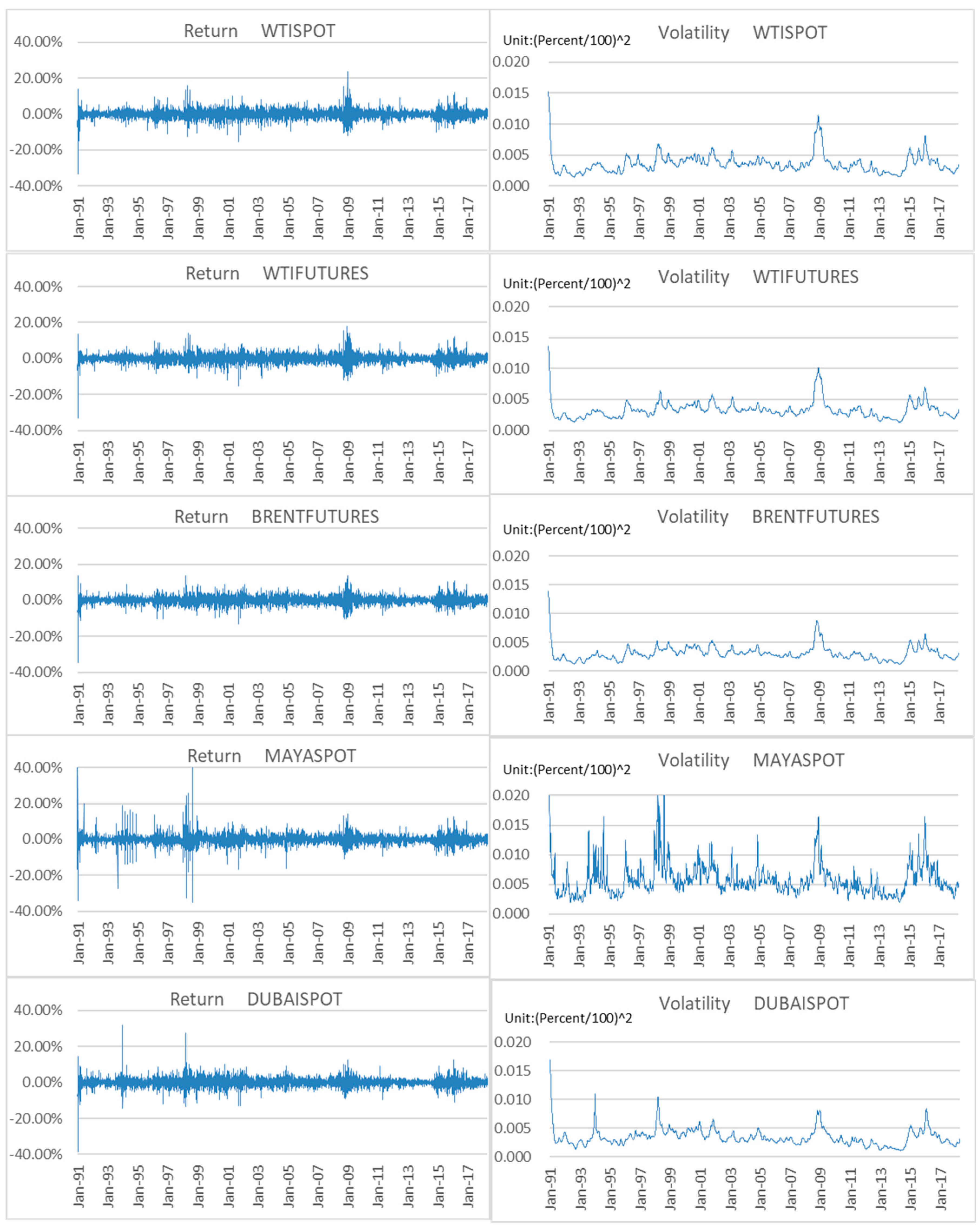
Figure 1 presents the time series plot of our data. We analyze model volatility by estimating a stochastic volatility model. (Let be a return with mean zero and variance . The SV model can be expressed as follows: where and are the level of log variance, the persistence of log variance, and the volatility of log variance, respectively. For the method of estimating the above equation, see Kastner and Frühwirth-Schnatter [36]. Yang and Hamori [37] compared the performance between GARCH and SV models for analyzing international agricultural commodities prices.) The figure indicates that the volatility of Maya spot is higher than in the other markets. The decrease in demand triggered by the Asian currency crisis in July 1997 and OPEC’s postponement of production cuts indirectly affected the Maya spot markets.
Table 2a,b presents the descriptive statistics for the daily change rate and volatility in crude oil prices. We use the Jarque–Bera statistics developed by Jarque and Bera [38] as test statistics for skewness and kurtosis to check whether the returns and volatility of crude oil prices are normally distributed. The test statistics reject normality at the 1% significance level for all variables. Table 2 also reports the results of the unit roots tests. To ensure that all variables are stationary, we adopt the Phillips–Perron (PP) tests developed by Phillips and Perron [39] and augmented Dickey Fuller (ADF) test developed by Said and Dickey [40]. The results show the null hypothesis that each variable with a unit root is rejected for both the PP and ADF tests for all variables.
4. Estimation Results
4.1. Spillover Results
Following Diebold and Yilmaz [3,30,31] and Barunik and Krehlik [33], we first estimate a five-variable VAR model based on the lag-length selection using the Schwarz–Bayesian information criterion (SBIC) developed by Schwarz [41]. Table 3 indicates the spillover table and time-frequency spillover results for returns, while Table 4 indicates the spillover table and time-frequency spillover results for volatility. Table 3 and Table 4 each consist of four sub-tables. From the top, the spillover table of Diebold and Yilmaz [3,30,31], and the short-term, medium-term, and long-term spillover results of Barunik and Krehlik [33] are placed in order. Tiwari et al. [42] analyze the volatility spillovers across global asset classes (global stock markets, CDS markets, foreign exchange markets, and sovereign bond markets) using a similar table. The first sub-table indicates the spillover table in the time domain. We decompose it into three frequencies, which are shown in the second, third, and fourth sub-tables. The sub-table “Freq S” roughly corresponds to a time frame of 1 to 5 days (short-term), while “Freq M” roughly corresponds to 5 to 21 days (medium-term), and “Freq L” roughly corresponds to 21 days to infinity (long-term). Values in the i-th row and the j-th column indicate the strength of spillover effect from the i-th market to the j-th market. The abbreviation “abs” means “absolute” and “wtn” means “within”. As for these differences, see Equations (12) and (13).
As Table 3 shows, the total connectedness of returns is 9.64%, which indicates that the returns on crude oil markets are not more closely linked with each other than the volatilities of the markets described later. From the Diebold and Yilmaz [3] spillover table, we find that the Dubai spot market (4.35%) contributes the most in the system, followed by the WTI spot (1.55%), Maya spot (1.44%), Brent futures (1.28%), and WTI futures markets (1.02%).
In addition, following Barunik and Krehlik [33], we decompose the Diebold and Yilmaz [3,30,31] spillover table based on frequencies. The results show that the total spillover from the short-term frequency (Freq S, 1 to 5 days; 8.17%) contributes the most to total connectedness, followed by the medium-term (Freq M, 5 to 21 days; 1.13%) and long-term (Freq L, more than 21 days; 0.34%) frequencies. Note that the total connectedness (9.64) is equal to the sum of the connectedness of each frequency, that is, 8.17 for Freq S, 1.13 for Freq M, and 0.34 for Freq L in Table 3.
As Table 4 shows, the total connectedness of volatilities is 48.72%. From the Diebold and Yilmaz [3] spillover table, we find that the WTI spot market (15.41%) contributes the most in the system, followed by the Brent futures (12.39%), Maya spot (8.48%), Dubai spot (7.04%), and WTI futures markets (5.41%). It is surprising that the WTI futures market, which is a common indicator of crude oil indices, contributes the least to both returns and volatility spillovers. The results also show that the total spillover from long-term frequency (47.66%) contributes the most to the total connectedness, followed by the medium-term (0.84%) and short-term (0.22%) frequencies. Furthermore, note that the total connectedness (48.72) is equal to the sum of the connectedness of each frequency, that is, 0.22 for Freq S, 0.84 for Freq M, and 47.66 for Freq L in Table 4.
It is interesting to see that the total connectedness among the five markets for returns is higher in the short-term than in the long-term. However, for volatility, this value is higher in the long-term than in the short-term.
4.2. Moving-Window Analysis
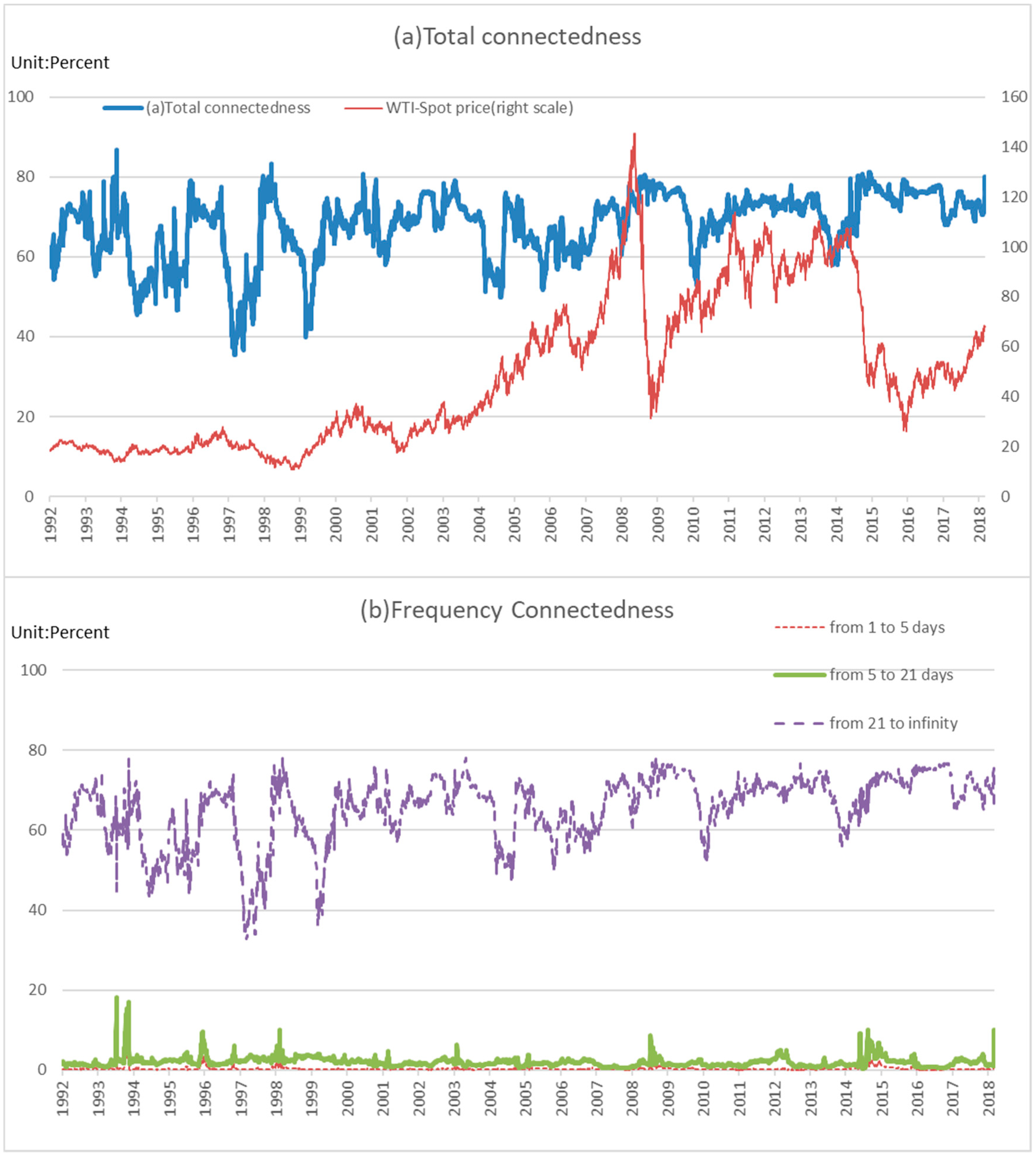
A lot of changes took place during the years in our sample, 1991–2018. Some examples include the Asian currency crisis around 1997, the global financial crisis in 2007–2008, the European sovereign debt crisis in 2009–2010, and Brexit in 2016. Thus, it seems unlikely that any single fixed-parameter model would apply over the entire sample. Although the full-sample spillover tables provide a useful summary of average behavior, they may miss potentially important movements in spillovers over time. Thus, we conduct a moving-windows analysis to capture the time-varying connectedness considering a decomposition in time domain as suggested by Diebold and Yilmaz [3,30,31] and in frequency domain as suggested by Barunik and Krehlik [33]. We estimate the models using 100-day rolling samples, and we assess the nature of spillover variation over time. Figure 2 and Figure 3 indicate the dynamics of total connectedness and frequency decomposition for return and volatility, respectively. We can identify two main points from the rolling analyses.
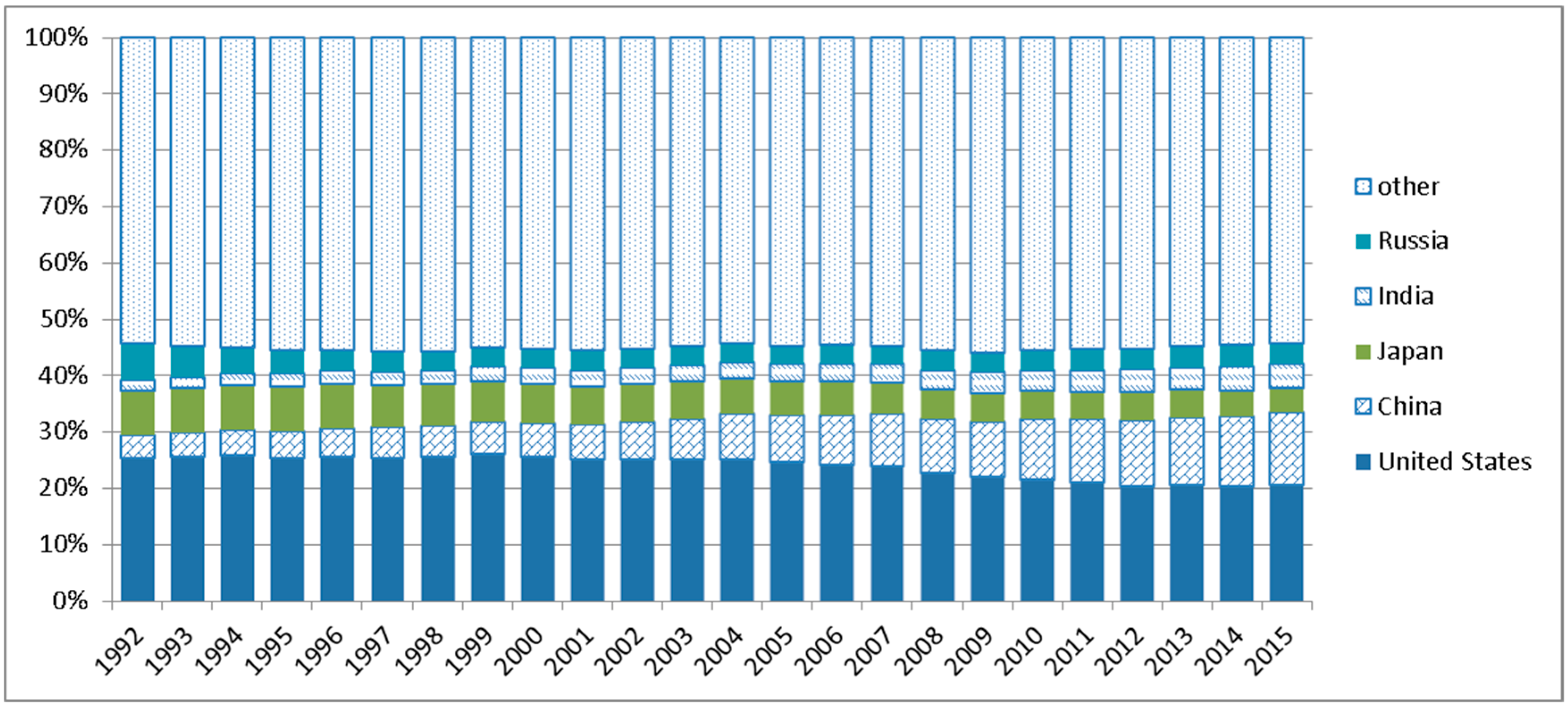
First, the total connectedness of returns has tended to strengthen since the mid-2000s. This roughly corresponds to the term during which consumption in China increased, arising from its rapid economic growth, indicated by Figure 4. On the other hand, we find no noticeable change in the total connectedness of volatility from 1991 to April 2018.
Next, the major events that occurred between 1991 and April 2018 were the Asian currency crisis (1997–1998) and the global financial crisis (2007–2008), which caused the rise in total connectedness of returns and volatilities. In recent years, especially since 2014, oil demand in emerging countries such as China has been sluggish. However, oil prices are increasing steadily; oil production in Russia, Brazil, and other non-OPEC oil-producing countries continues; and shale oil production in the US continues to expand rapidly. Therefore, the market saw an oversupply of crude oil, which caused a sharp fall in prices. In addition, due to this sharp fall in prices, the total connectedness of volatility remained at a high level, but the total connectedness of returns fell.
5. Concluding Remarks
This study analyzes return and volatility spillovers across global crude oil markets for 1 January 1991 to 27 April 2018 using an empirical technique for the time and frequency domains developed by Barunik and Krehlik [33]. This study makes four contributions to the literature.
First, the spillover tables reveal that the WTI futures market, which is a common indicator of crude oil indices, contributed the least to spillovers in both returns and volatility. Conversely, Dubai spot contributed the most to return spillover. This result is consistent with Kaufmann and Ullman [17].
Second, these results also show that the short-term factor contributed the most to return spillover, while the long-term factor contributed the most to volatility. As for the volatility spillover, this result is consistent with Barunik et al. [4].
Third, the rolling analyses show that the total connectedness of returns has tended to strengthen since the mid-2000s. This roughly corresponds to the term during which consumption in China increased, arising from its rapid economic growth. On the other hand, we find no noticeable change in total connectedness of volatility from 1991 to April 2018.
Finally, the major events that occurred between 1991 and April 2018, namely the Asian currency crisis (1997–1998) and the global financial crisis (2007–2008), caused the rise in total connectedness of returns and volatilities. In recent years, especially since 2014, oil demand in emerging countries such as China has been sluggish, though oil prices are increasing steadily; oil production in Russia, Brazil, and other non-OPEC oil-producing countries continues; and shale oil production in the US continues to expand rapidly. Therefore, crude oil was oversupplied, which caused the sharp fall in prices. In addition, due to this sharp fall in prices, the total connectedness of volatility remained at a high level, but the total connectedness of returns fell.
Author Contributions
Data curation, Y.T.; formal analysis, Y.T.; writing—original draft preparation, Y.T.; writing—review and editing, S.H.; supervision, S.H.
Funding
This work was supported by JSPS KAKENHI, grant nos. 17K18564 and 17H00983.
Acknowledgments
We are grateful to two anonymous referees for their helpful comments and suggestions.
Conflicts of Interest
The authors declare no conflict of interest.
References
- Ross, S.A. Information and volatility: No-arbitrage martingale approach to timing and resolution irrelevancy. J. Financ. 1989, 44, 1–17. [Google Scholar] [CrossRef]
- Fleming, J.; Kirby, C.; Ostdiek, B. Information and volatility linkages in the stock, bond, and money markets. J. Financ. Econ. 1998, 49, 111–137. [Google Scholar] [CrossRef]
- Diebold, F.X.; Yilmaz, K. Better to give than receive: Predictive directional measurement of volatility spillovers. Int. J. Forecast. 2012, 28, 57–66. [Google Scholar] [CrossRef]
- Barunik, J.; Koenda, E.; Vácha, L. Asymmetric connectedness of stocks: Bad and good volatility spillovers. J. Financ. Mark. 2016, 27, 55–78. [Google Scholar] [CrossRef]
- Bae, K.H.; Karolyi, A.; Stulz, R. A new approach to measuring financial contagion. Rev. Financ. Stud. 2003, 16, 717–763. [Google Scholar] [CrossRef]
- Dungey, M.; Martin, V.L. Unravelling financial market linkages during crises. J. Appl. Econom. 2007, 22, 89–199. [Google Scholar] [CrossRef]
- Morana, C.; Beltratti, A. Comovements in international stock markets. J. Int. Financ. Mark Inst. Money 2008, 18, 31–45. [Google Scholar] [CrossRef]
- Ehrmann, M.; Fratzscher, M.; Rigobon, R. Stocks, bonds, money markets and exchange rates: Measuring international financial transmission. J. Appl. Econom. 2011, 26, 948–974. [Google Scholar] [CrossRef]
- Beirne, J.; Gieck, J. Interdepencence and contagion in global asset markets. Rev. Int. Econ. 2014, 22, 639–659. [Google Scholar] [CrossRef]
- Bae, K.H.; Zhang, X. The cost of stock market integration in emerging markets. Asia Pac. J. Financ. Stud. 2015, 44, 1–23. [Google Scholar] [CrossRef]
- Lehkonen, H. Stock market integration and the global financial crisis. Rev. Financ. 2015, 19, 2039–2094. [Google Scholar] [CrossRef]
- Aït-Sahalia, Y.; Hurd, T. Portfolio choice in markets with contagion. J. Financ. Econom. 2016, 14, 1–28. [Google Scholar] [CrossRef]
- Ang, A.; Bekaert, G. International asset allocation with regime shifts. Rev. Financ. Stud. 2002, 15, 1137–1187. [Google Scholar] [CrossRef]
- Balcilar, M.; Demirer, R.; Hammoudeh, S.; Nguyen, D.K. Risk spillovers across the energy and carbon markets and hedging strategies for carbon risk. Energy Econ. 2016, 54, 159–172. [Google Scholar] [CrossRef] [Green Version]
- Scholes, M.S. Crisis and risk management. Am. Econ. Rev. 2000, 90, 17–21. [Google Scholar] [CrossRef]
- Chang, C.P.; Lee, C.C. Do oil spot and futures move together? Energy Econ. 2015, 50, 379–390. [Google Scholar] [CrossRef]
- Kaufmann, R.K.; Ullman, B. Oil prices, speculation, and fundamentals: Interpreting causal relations among spot and futures prices. Energy Econ. 2009, 31, 550–558. [Google Scholar] [CrossRef]
- Pan, Z.; Wang, Y.; Yan, L. Hedging crude oil using refined product: A regime switching asymmetric DCC approach. Energy Econ. 2014, 46, 472–484. [Google Scholar] [CrossRef]
- Chang, C.L.; McAleer, M.; Tansuchat, R. Crude oil hedging strategies using dynamic multivariate GARCH. Energy Econ. 2011, 33, 912–923. [Google Scholar] [CrossRef] [Green Version]
- Toyoshima, Y.; Nakajima, T.; Hamori, S. Crude oil hedging strategy: New evidence from the data of the financial crisis. Appl. Financ. Econ. 2013, 23, 1033–1041. [Google Scholar] [CrossRef]
- Nicolau, M.; Palomba, G. Dynamic relationships between spot and futures prices: The case of energy and gold commodities. Resour. Policy 2015, 45, 130–143. [Google Scholar] [CrossRef]
- Chen, P.F.; Lee, C.C.; Zeng, J.H. The relationships between spot and futures oil prices: Do structural breaks matter? Energy Econ. 2014, 43, 206–217. [Google Scholar] [CrossRef]
- Wang, Y.; Wu, C. Are crude oil spot and futures prices cointegrated? Not always! Econ. Model. 2013, 33, 641–650. [Google Scholar] [CrossRef]
- Maslyuk, S.; Smyth, R. Cointegration between oil spot and future prices of the same and different grades in the presence of structural change. Energy Policy 2009, 37, 1687–1693. [Google Scholar] [CrossRef]
- Huang, B.N.; Yang, C.W.; Hwang, M.J. The dynamics of a nonlinear relationship between crude oil spot and futures prices: A multivariate threshold regression approach. Energy Econ. 2009, 31, 91–98. [Google Scholar] [CrossRef]
- Bekiros, S.D.; Diks, C.G.H. The relationship between crude oil spot and futures prices: Cointegration, linear, and nonlinear causality. Energy Econ. 2008, 30, 2673–2685. [Google Scholar] [CrossRef]
- Bhar, R.; Hamori, S. Causality in variance and the type of traders in crude oil futures. Energy Econ. 2005, 27, 527–539. [Google Scholar] [CrossRef]
- Lee, C.C.; Zeng, J.H. The impact of oil price shocks on stock market activities: Asymmetric effect with quantile regression. Math. Comput. Simul. 2011, 81, 1910–1920. [Google Scholar] [CrossRef]
- Balcilar, M.; Bekiros, S.; Gupta, R. The role of news-based uncertainty indices in predicting oil markets: A hybrid nonparametric quantile causality method. Empir. Econ. 2017, 53, 879–889. [Google Scholar] [CrossRef]
- Yun, W.C.; Kim, H.J. Hedging strategy for crude oil trading and the factors influencing hedging effectiveness. Energy Policy 2010, 38, 2404–2408. [Google Scholar] [CrossRef]
- Diebold, F.X.; Yilmaz, K. Financial and Macroeconomic Connectedness: A Network Approach to Measurement and Monitoring, 1st ed.; Oxford University Press: Oxford, UK, 2014. [Google Scholar]
- Diebold, F.X.; Yilmaz, K. Measuring financial asset return and volatility spillovers, with application to global equity markets. Econ. J. 2009, 119, 158–171. [Google Scholar] [CrossRef]
- Barunik, J.; Krehlik, T. Measuring the frequency dynamics of financial connectedness and systemic risk. J. Financ. Econom. 2018, 16, 271–296. [Google Scholar] [CrossRef]
- Koop, G.; Pesaran, M.H.; Potter, S.M. Impulse Response Analysis in Nonlinear Multivariate Models. J. Econom. 1996, 74, 119–147. [Google Scholar] [CrossRef]
- Pesaran, H.H.; Shin, Y. Generalized Impulse Response Analysis in Linear Multivariate Models. Econ. Lett. 1998, 58, 17–29. [Google Scholar] [CrossRef]
- Kastner, G.; Frühwirth-Schnatter, S. Ancillarity-sufficiency interweaving strategy (ASIS) for boosting MCMC estimation of stochastic volatility models. Comput. Stat. Data Anal. 2014, 76, 408–423. [Google Scholar] [CrossRef] [Green Version]
- Yang, L.; Hamori, S. Modeling the dynamics of international agricultural commodity prices: A comparison of GARCH and stochastic volatility models. Ann. Financ. Econ. 2018, 13, 1850010. [Google Scholar] [CrossRef]
- Jarque, C.M.; Bera, A.K. Test for normality of observations and regression residuals. Int. Stat. Rev. 1987, 55, 163–172. [Google Scholar] [CrossRef]
- Phillips, P.C.B.; Perron, P. Testing for a unit root in time series regression. Biometrika 1988, 75, 335–346. [Google Scholar] [CrossRef]
- Said, S.E.; Dickey, D.A. Testing for unit roots in autoregressive-moving average models of unknown order. Biometrika 1984, 71, 599–607. [Google Scholar] [CrossRef]
- Schwarz, G. Estimating the dimension of a model. Ann. Stat. 1978, 6, 461–464. [Google Scholar] [CrossRef]
- Tiwari, A.K.; Cunado, J.; Gupta, R.; Wohar, M.E. Volatility spillovers across global asset classes: Evidence from time and frequency domains. Q. Rev. Econ. Financ. 2018. [Google Scholar] [CrossRef]
- Kilian, L. Not all oil price shocks are alike: Disentangling demand and supply shocks in the crude oil market. Am. Econ. Rev. 2009, 99, 1053–1069. [Google Scholar] [CrossRef]
- Chen, W.; Kinkyo, T.; Hamori, S. Macroeconomic Impacts of Oil Prices and Underlying Financial Shocks. J. Int. Financ. Mark. Inst. Money 2014, 29, 1–12. [Google Scholar] [CrossRef]
Figure 1.
Time series plots of returns and volatility. Data Source: Bloomberg: WTISPOT: West Texas Intermediate (WTI) crude oil spot price; WTIFUTURES: WTI crude oil futures price; BRENTFUTURES: Brent crude oil futures price; MAYASPOT: Maya crude oil spot price; DUBAISPOT: Dubai crude oil spot price.

Figure 2.
Dynamic frequency connectedness for returns.

Figure 3.
Dynamic frequency connectedness for volatilities.

Figure 4.
Share of consumption. Data source: US Energy Information Administration.


Table 1.
Previous studies and their main contributions.
| No. | Authors | Journal Name | Empirical Technique | Market/Data | Principal Results |
|---|---|---|---|---|---|
| 16 | Chang and Lee (2015) | Energy Economics | Wavelet coherency analysis in time–frequency domain | WTI spot and futures | Long-run cointegration relationship between oil spot and futures prices is found. In addition, the short-run causality is more significant in shorter maturity pairs. |
| 17 | Kaufmann and Ullman (2009) | Energy Economics | Unrestricted vector error correction model (VECM) | WTI spot and futures Brent spot and futures Maya spot Dubai-Fateh spot Bonny light spot | Innovations of spillover first appear in spot prices for Dubai–Fateh and spread to other spot and futures prices while other innovations first appear in the far month contract for West Texas Intermediate and spread to other exchanges and contracts. |
| 18 | Pan et al. (2014) | Energy Economics | Regime switching asymmetric dynamic conditional correlation (DCC) model | WTI spot and futures gasoline and heating oil | To hedge portfolio, regime switching asymmetric DCC model is better model than some conventional multivariate generalized autoregressive conditional heteroscedasticity model (multivariate GARCH model). |
| 19 | Chang et al. (2011) | Energy Economics | Multivariate GARCH | WTI spot and futures | To calculate optimal portfolio weights and optimal hedge ratios, diagonal Baba-Engle-Kraft-Kroner (diagonal BEKK) model is the best model. |
| 20 | Toyoshima et al. (2013) | Applied Financial Economics | Asymmetric DCC Multivariate GARCH | WTI spot and futures | To reduce the variance of hedged portfolio, the performance of models is good in order of Asymmetric DCC, DCC, and Diagonal BEKK. |
| 21 | Nicolau (2015) | Resources Policy | Recursive bivariate VAR model | WTI spot and futures | Cointegration relationship between oil spot and futures prices is found, and weak exogeneity exists. |
| 22 | Chen et al. (2014) | Energy Economics | Cointegration tests with structural breaks | WTI spot and futures | Authors find one structural break (July 2004) existed in the long-run relationship between spot and futures oil prices. |
| 23 | Wang and Wu (2013) | Economic Modelling | Nonlinear threshold VECM | WTI spot and futures | Cointegration relationship between crude oil spot and futures are found only when the price differentials are larger than the threshold value |
| 24 | Maslyuk and Smyth (2009) | Energy Policy | Residual-based tests for cointegration in models with regime shifts | WTI and Brent spot and futures | Spot and future prices of the same grade as well as spot and futures prices of different grades are cointegrated. |
| 25 | Huang et al. (2009) | Energy Economics | Three-regime VECM | WTI spot and futures | When the spot price is higher than futures price, and the basis is less than certain threshold value, there exists at least one causal relationship between the change of spot price and futures price. |
| 26 | Bekiros and Diks (2008) | Energy Economics | Linear Granger test nonlinear causality test | WTI spot and futures | While the linear causal relationships have disappeared after the cointegration filtering, nonlinear causal linkages in some cases were revealed. |
| 27 | Bhar and Hamori (2005) | Energy Economics | Cross-correlation function approach | Crude oil futures price Crude oil trading volume | One-way causal effect from price to volume in the investigation of crude oil futures market is found. |
| 28 | Lee and Zeng (2011) | Mathematics and Computers in Simulation | Multiple structural breaks test Quantile regression | Average global crude oil price Real stock returns in G7 countries Interest rate Industrial production | The responses of stock markets to oil price shocks are diverse among G7 countries.In many cases, quantile regression estimates are quite different from simple ordinary least squares (OLS) models. |
| 29 | Balcilar et al. (2017) | Empirical Economics | Nonparametric quantile causality test | WTI spot Economic policy uncertainty (EPU) index Equity market uncertainty (EMU) index | For oil returns, EPU and EMU have strong predictive power over the entire distribution barring regions around the median, but for volatility, the predictability virtually covers the entire distribution, with some exceptions in the tails. |
| 30 | Yun et al. (2010) | Energy Policy | Simple OLS | Dubai spot and WTI futures Exchange rate | Authors find that the hedging effectiveness would be improved by considering the intercorrelation between commodity price and exchange rate. |
Table 2.
Descriptive statistics and preliminary tests for return and volatility.
| a. Descriptive Statistics and Preliminary Tests for Return. | |||||
| Return WTISPOT | Return WTIFUTURES | Return BRENTFUTURES | Return MAYASPOT | Return DUBAISPOT | |
| Observations | 7128 | 7128 | 7128 | 7128 | 7128 |
| Descriptive statistics | |||||
| Mean | 0.040% | 0.038% | 0.036% | 0.054% | 0.042% |
| Median | 0.000% | 0.000% | 0.000% | 0.000% | 0.000% |
| Maximum | 23.709% | 17.833% | 13.767% | 50.330% | 31.757% |
| Minimum | –33.519% | –33.000% | –34.768% | –34.942% | –38.697% |
| Std. Dev. | 2.341% | 2.282% | 2.125% | 2.651% | 2.328% |
| Skewness | –0.180 | –0.227 | –0.518 | 1.195 | –0.032 |
| Kurtosis | 14.487 | 13.688 | 16.458 | 56.240 | 24.376 |
| Normality tests | |||||
| Jarque-Bera | 39,227.840 | 33,991.800 | 54,109.080 | 843,541.300 | 135,714.100 |
| Probability | 0.000 | 0.000 | 0.000 | 0.000 | 0.000 |
| Unit root tests | |||||
| ADF test statistics | –85.810 | –86.409 | –87.795 | –90.269 | –64.635 |
| p-value | 0.000 | 0.000 | 0.000 | 0.000 | 0.000 |
| PP test statistics | –86.438 | –86.858 | –87.832 | –90.132 | –91.714 |
| p-value | 0.000 | 0.000 | 0.000 | 0.000 | 0.000 |
| b. Descriptive Statistics and Preliminary Tests for Volatility. | |||||
| Volatility WTISPOT | Volatility WTIFUTURES | Volatility BRENTFUTURES | Volatility MAYASPOT | Volatility DUBAISPOT | |
| Observations | 7128 | 7128 | 7128 | 7128 | 7128 |
| Descriptive statistics | |||||
| Mean | 0.004 | 0.003 | 0.003 | 0.006 | 0.003 |
| Median | 0.003 | 0.003 | 0.003 | 0.005 | 0.003 |
| Maximum | 0.015 | 0.014 | 0.014 | 0.039 | 0.017 |
| Minimum | 0.001 | 0.001 | 0.001 | 0.002 | 0.001 |
| Std. Dev. | 0.001 | 0.001 | 0.001 | 0.003 | 0.001 |
| Skewness | 2.388 | 2.292 | 2.190 | 3.003 | 2.235 |
| Kurtosis | 12.943 | 12.123 | 13.197 | 21.213 | 13.435 |
| Normality tests | |||||
| Jarque-Bera | 36,139.550 | 30,960.240 | 36,577.650 | 109,230.200 | 38,273.380 |
| Probability | 0.000 | 0.000 | 0.000 | 0.000 | 0.000 |
| Unit root tests | |||||
| ADF test statistics | –7.915 | –6.811 | –8.466 | –11.440 | –8.407 |
| p-value | 0.000 | 0.000 | 0.000 | 0.000 | 0.000 |
| PP test statistics | –8.405 | –8.376 | –9.106 | –12.356 | –9.117 |
| p-value | 0.000 | 0.000 | 0.000 | 0.000 | 0.000 |
Note: WTISPOT: WTI crude oil spot price; WTIFUTURES: WTI crude oil futures price; BRENTFUTURES: Brent crude oil futures price; MAYASPOT: Maya crude oil spot price; DUBAISPOT: Dubai crude oil spot price.
Table 3.
Returns spillover results.
| Diebold and Yilmaz (2012) Spillover Table | |||||||
| Return WTISPOT | Return WTIFUTURES | Return BRENTFUTURES | Return MAYASPOT | Return DUBAISPOT | From | ||
| Return WTISPOT | 92.25 | 6.86 | 0.37 | 0.13 | 0.39 | 1.55 | |
| Return WTIFUTURES | 2.96 | 94.89 | 1.35 | 0.12 | 0.67 | 1.02 | |
| Return BRENTFUTURES | 3.14 | 2.71 | 93.59 | 0.28 | 0.29 | 1.28 | |
| Return MAYASPOT | 2.26 | 2.55 | 2.19 | 92.81 | 0.20 | 1.44 | |
| Return DUBAISPOT | 2.74 | 1.99 | 16.42 | 0.60 | 78.25 | 4.35 | |
| To | 2.22 | 2.82 | 4.07 | 0.23 | 0.31 | 9.64 | |
| Barunik and Krehlik (2018) Spillover results | |||||||
| Freq S: The Spillover Table for Band: 3.14 to 0.63. Roughly Corresponds to 1 Days to 5 Days. | |||||||
| Return WTISPOT | Return WTIFUTURES | Return BRENTFUTURES | Return MAYASPOT | Return DUBAISPOT | From_abs | From_wtn | |
| Return WTISPOT | 83.78 | 5.26 | 0.32 | 0.13 | 0.29 | 1.2 | 1.33 |
| Return WTIFUTURES | 2.66 | 85.39 | 0.78 | 0.12 | 0.57 | 0.82 | 0.92 |
| Return BRENTFUTURES | 2.84 | 2.66 | 80.79 | 0.23 | 0.28 | 1.20 | 1.33 |
| Return MAYASPOT | 2.21 | 2.30 | 1.51 | 84.21 | 0.17 | 1.24 | 1.37 |
| Return DUBAISPOT | 2.38 | 1.97 | 13.75 | 0.47 | 75.16 | 3.71 | 4.12 |
| To_abs | 2.02 | 2.44 | 3.27 | 0.19 | 0.26 | 8.17 | |
| To_wtn | 2.24 | 2.71 | 3.63 | 0.21 | 0.29 | 9.08 | |
| Freq M: The Spillover Table for Band: 0.63 to 0.15. Roughly Corresponds to 5 Days to 21 Days. | |||||||
| Return WTISPOT | Return WTIFUTURES | Return BRENTFUTURES | Return MAYASPOT | Return DUBAISPOT | From_abs | From_wtn | |
| Return WTISPOT | 6.78 | 1.26 | 0.03 | 0.00 | 0.08 | 0.27 | 3.57 |
| Return WTIFUTURES | 0.25 | 7.33 | 0.43 | 0.00 | 0.09 | 0.15 | 1.99 |
| Return BRENTFUTURES | 0.25 | 0.05 | 9.72 | 0.04 | 0.01 | 0.07 | 0.88 |
| Return MAYASPOT | 0.04 | 0.19 | 0.49 | 6.40 | 0.02 | 0.15 | 1.94 |
| Return DUBAISPOT | 0.29 | 0.03 | 2.04 | 0.09 | 2.49 | 0.49 | 6.37 |
| To_abs | 0.16 | 0.30 | 0.60 | 0.03 | 0.04 | 1.13 | |
| To_wtn | 2.15 | 3.97 | 7.77 | 0.36 | 0.51 | 14.76 | |
| Freq L: The Spillover Table for Band: 0.15 to 0.01. Roughly Corresponds to More than 21 Days. | |||||||
| Return WTISPOT | Return WTIFUTURES | Return BRENTFUTURES | Return MAYASPOT | Return DUBAISPOT | From_abs | From_wtn | |
| Return WTISPOT | 1.70 | 0.34 | 0.02 | 0.00 | 0.02 | 0.08 | 3.29 |
| Return WTIFUTURES | 0.06 | 2.17 | 0.14 | 0.00 | 0.02 | 0.05 | 1.92 |
| Return BRENTFUTURES | 0.05 | 0.00 | 3.07 | 0.01 | 0.00 | 0.01 | 0.64 |
| Return MAYASPOT | 0.01 | 0.06 | 0.19 | 2.20 | 0.01 | 0.05 | 2.31 |
| Return DUBAISPOT | 0.07 | 0.00 | 0.64 | 0.03 | 0.61 | 0.15 | 6.49 |
| To_abs | 0.04 | 0.08 | 0.20 | 0.01 | 0.01 | 0.34 | |
| To_wtn | 1.65 | 3.47 | 8.62 | 0.45 | 0.45 | 14.64 | |
Note 1: WTISPOT: WTI crude oil spot price; WTIFUTURES: WTI crude oil futures price; BRENTFUTURES: Brent crude oil futures price; MAYASPOT: Maya crude oil spot price; DUBAISPOT: Dubai crude oil spot price. Note 2: Values in the i-th row of the j-th column indicate the strength of spillover effect from the i-th market to the j-th market. abs, absolute; wtn, within. For these differences, see Equations (12) and (13).
Table 4.
Volatility spillover results.
| Diebold and Yilmaz (2012) Spillover Table | |||||||
| Volatility WTISPOT | Volatility WTIFUTURES | Volatility BRENTFUTURES | Volatility MAYASPOT | Volatility DUBAISPOT | From | ||
| Volatility WTISPOT | 22.96 | 49.32 | 12.72 | 8.02 | 6.98 | 15.41 | |
| Volatility WTIFUTURES | 6.19 | 72.96 | 9.00 | 7.96 | 3.88 | 5.41 | |
| Volatility BRENTFUTURES | 1.41 | 47.90 | 38.04 | 5.95 | 6.71 | 12.39 | |
| Volatility MAYASPOT | 3.83 | 14.53 | 6.04 | 57.62 | 17.98 | 8.48 | |
| Volatility DUBAISPOT | 2.64 | 20.60 | 8.63 | 3.32 | 64.81 | 7.04 | |
| To | 2.82 | 26.47 | 7.28 | 5.05 | 7.11 | 48.72 | |
| Barunik and Krehlik (2018) Spillover results | |||||||
| Freq S: The Spillover Table for Band: 3.14 to 0.63. Roughly Corresponds to 1 Days to 5 Days. | |||||||
| Volatility WTISPOT | Volatility WTIFUTURES | Volatility BRENTFUTURES | Volatility MAYASPOT | Volatility DUBAISPOT | From_abs | From_wtn | |
| Volatility WTISPOT | 0.06 | 0.28 | 0.04 | 0.03 | 0.02 | 0.07 | 21.63 |
| Volatility WTIFUTURES | 0.00 | 0.12 | 0.02 | 0.03 | 0.01 | 0.01 | 3.95 |
| Volatility BRENTFUTURES | 0.01 | 0.30 | 0.01 | 0.03 | 0.01 | 0.07 | 19.73 |
| Volatility MAYASPOT | 0.02 | 0.07 | 0.01 | 0.43 | 0.02 | 0.03 | 7.32 |
| Volatility DUBAISPOT | 0.02 | 0.13 | 0.02 | 0.01 | 0.02 | 0.04 | 10.56 |
| To_abs | 0.01 | 0.15 | 0.02 | 0.02 | 0.01 | 0.22 | |
| To_wtn | 2.92 | 45.04 | 5.61 | 6.00 | 3.62 | 63.19 | |
| Freq M: The Spillover Table for Band: 0.63 to 0.15. Roughly Corresponds to 5 Days to 21 Days. | |||||||
| Volatility WTISPOT | Volatility WTIFUTURES | Volatility BRENTFUTURES | Volatility MAYASPOT | Volatility DUBAISPOT | From_abs | From_wtn | |
| Volatility WTISPOT | 0.59 | 0.80 | 0.13 | 0.04 | 0.08 | 0.21 | 5.34 |
| Volatility WTIFUTURES | 0.07 | 0.27 | 0.08 | 0.04 | 0.03 | 0.04 | 1.11 |
| Volatility BRENTFUTURES | 0.04 | 0.85 | 0.18 | 0.03 | 0.04 | 0.19 | 4.97 |
| Volatility MAYASPOT | 0.28 | 0.64 | 0.19 | 14.01 | 0.27 | 0.28 | 7.07 |
| Volatility DUBAISPOT | 0.09 | 0.38 | 0.08 | 0.02 | 0.35 | 0.11 | 2.90 |
| To_abs | 0.10 | 0.53 | 0.10 | 0.03 | 0.08 | 0.84 | |
| To_wtn | 2.46 | 13.63 | 2.45 | 0.72 | 2.12 | 21.38 | |
| Freq L: The Spillover Table for Band: 0.15 to 0.01. Roughly Corresponds to More than 21 Days. | |||||||
| Volatility WTISPOT | Volatility WTIFUTURES | Volatility BRENTFUTURES | Volatility MAYASPOT | Volatility DUBAISPOT | From_abs | From_wtn | |
| Volatility WTISPOT | 22.31 | 48.24 | 12.56 | 7.94 | 6.89 | 15.13 | 15.8 |
| Volatility WTIFUTURES | 6.12 | 72.57 | 8.90 | 7.89 | 3.84 | 5.36 | 5.59 |
| Volatility BRENTFUTURES | 1.36 | 46.75 | 37.86 | 5.89 | 6.66 | 12.13 | 12.67 |
| Volatility MAYASPOT | 3.53 | 13.81 | 5.84 | 43.18 | 17.68 | 8.17 | 8.54 |
| Volatility DUBAISPOT | 2.53 | 20.10 | 8.53 | 3.28 | 64.44 | 6.89 | 7.2 |
| To_abs | 2.71 | 25.79 | 7.16 | 5.00 | 7.02 | 47.66 | |
| To_wtn | 2.83 | 26.93 | 7.48 | 5.22 | 7.33 | 49.79 | |
Note 1: WTISPOT: WTI crude oil spot price; WTIFUTURES: WTI crude oil futures price; BRENTFUTURES: Brent crude oil futures price; MAYASPOT: Maya crude oil spot price; DUBAISPOT: Dubai crude oil spot price. Note 2: Values in the i-th row of the j-th column indicate the strength of spillover effect from the i-th market to the j-th market. abs, absolute; wtn, within. For these differences, see Equations (12) and (13).
© 2018 by the authors. Licensee MDPI, Basel, Switzerland. This article is an open access article distributed under the terms and conditions of the Creative Commons Attribution (CC BY) license (http://creativecommons.org/licenses/by/4.0/).
Share and Cite
MDPI and ACS Style
Toyoshima, Y.; Hamori, S. Measuring the Time-Frequency Dynamics of Return and Volatility Connectedness in Global Crude Oil Markets. Energies 2018, 11, 2893. https://doi.org/10.3390/en11112893
AMA Style
Toyoshima Y, Hamori S. Measuring the Time-Frequency Dynamics of Return and Volatility Connectedness in Global Crude Oil Markets. Energies. 2018; 11(11):2893. https://doi.org/10.3390/en11112893
Chicago/Turabian StyleToyoshima, Yuki, and Shigeyuki Hamori. 2018. "Measuring the Time-Frequency Dynamics of Return and Volatility Connectedness in Global Crude Oil Markets" Energies 11, no. 11: 2893. https://doi.org/10.3390/en11112893
Note that from the first issue of 2016, this journal uses article numbers instead of page numbers. See further details here.