Fault-Tolerant Temperature Control Algorithm for IoT Networks in Smart Buildings

Abstract

The monitoring of the Internet of things networks depends to a great extent on the availability and correct functioning of all the network nodes that collect data. This network nodes all of which must correctly satisfy their purpose to ensure the efficiency and high quality of monitoring and control of the internet of things networks. This paper focuses on the problem of fault-tolerant maintenance of a networked environment in the domain of the internet of things. Based on continuous-time Markov chains, together with a cooperative control algorithm, a novel feedback model-based predictive hybrid control algorithm is proposed to improve the maintenance and reliability of the internet of things network. Virtual sensors are substituted for the sensors that the algorithm predicts will not function properly in future time intervals; this allows for maintaining reliable monitoring and control of the internet of things network. In this way, the internet of things network improves its robustness since our fault tolerant control algorithm finds the malfunction nodes that are collecting incorrect data and self-correct this issue replacing malfunctioning sensors with new ones. In addition, the proposed model is capable of optimising sensor positioning. As a result, data collection from the environment can be kept stable. The developed continuous-time control model is applied to guarantee reliable monitoring and control of temperature in a smart supermarket. Finally, the efficiency of the presented approach is verified with the results obtained in the conducted case study.

1. Introduction

The advances in communications techniques, network topologies and control methods, have contributed to the development of Networked Control Systems (NCSs), expanding their possibilities. As a result, in the last several decades, NCSs have received considerable attention form the scientific community, mainly due to their wide-ranging application possibilities [1]. Once an Internet of Things (IoT) network is formed by multiple IoT nodes, controller or actuator nodes, it is feasible for them to capture data from a large range of existing structures. However, when the accuracy of IoT nodes is reduced, the data they capture is faulty and causes inappropriate decisions. Therefore, it is critical to increase the ability of the IoT network to detect IoT nodes which are not operating properly [2]. This work introduces a new predictive temperature control algorithm for fault tolerant detection of a large number of IoT nodes, providing an efficient temperature control. The implementation of a system to control and monitor the precision states of the IoT nodes will ensure reliability of the data captured by the IoT network. The discrete time control focuses on system efficiency at a discrete time range rather than a continuous time range. The discrete-time control issues, such as linear systems have been investigated. Amato et al. deal with the finite-time stabilization of continuous-time linear systems is considered. The main result provided is a sufficient condition for the design of a dynamic output feedback controller which makes the closed loop system finite-time stable [3,4]. Therefore, Polyakov et al. consider the control design problem for finite-time and fixed-time stabilizations of linear multi-input system with nonlinear uncertainties and disturbances, so the robustness properties of the network are improved [5]. The works presented above show that the quality of any linear control algorithm is estimated by different performance indices such as robustness with respect to disturbances. Although these authors make their study in discrete time, the algorithm we have developed is an important starting point. Meanwhile, the studies on the discrete-time control of nonlinear system have also been carried out for triangular systems [6] or nonlinear dynamical networks [7]. These two papers have a different approach to the problem of discrete-time control. Korobov et al. solve the issue of global stabilization in finite-time for a general class of triangular multi-input multi-output $(MIMO)$ systems with singular input–output links combining the controllability function method with a modification of the global construction. Hui et al. focus on the analysis of semistability and stability in finite time and on the synthesis of systems with a continuous equilibrium. These two approaches address the problem of control in nonlinear systems in very specific cases of triangular and semi-stable systems. Although these are two rather limited case studies, they give a very good focus on how to deal with nonlinear control problems. Discrete-time control techniques have been applied for many practical applications, for instance, multi-agent systems [8] and secure communications [9]. Both works present a new adaptive fuzzy output feedback control approach composed for a type of nonlinear single input and single output feedback control systems with unmeasured status and input saturation. In these two works, we can see that fuzzy control is a good approach to the problem of nonlinear control, but the authors think that, for this case, it is an invalid technique, since all the control functions of the system are known. Feedback nonlinear systems representing a class of nonlinear control systems have been widely considered [10,11]. The problem we address is the topic of predictive maintenance of IoT networks in continuous-time, with the aim of increasing the monitoring and control reliability of IoT networks, as it is done in continuous-time. By using continuous-time Markov chains to predict the future accuracy states of sensors, IoT networks will collect quality data because their nodes will always work in an optimal state.

Motivated by the above observation, this paper proposes a new feedback control algorithm to improve predictive maintenance of the IoT networks. The algorithm finds the IoT nodes that do not function correctly and collect false data. To optimize the monitoring and control processes of the IoT network, a novel application of the continuous-time Markov chains is used. We predict the future accuracy states of the IoT nodes and, in case it is predicted that a sensor will become faulty after the time control period has expired, the controller sends a signal that this IoT node has to be replaced. Moreover, if an IoT node has to be replaced, the control algorithm creates a virtual sensor in that position. This virtual sensor estimates the temperature of that sensor based on the temperature of its neighboring nodes. In this way, the IoT network collects data in continuous-time range without any loss of reliability in the data due to malfunctions in the IoT devices.

The problem of data quality and the detecting of incorrect data has been extensively studied [12]; these works search the quality of data applying different techniques as game theory [13] or other types of metrics [14]. These articles provide a solid design of how to increase the quality of data; in our opinion, these works are focused on homogeneous data and discrete time; even so, they are an excellent support for our research. The above-mentioned studies on data quality and detection of incorrect data concern discrete time, and the outputs for continuous time systems are quite limited. Actually, continuous time control systems have been applied in a large range of fields, such as feedback control of nonlinear systems [15,16]. These papers deal with the stability of discrete-time networked systems with multiple sensor nodes under dynamic scheduling protocols. In fact, this is a great advancement for the stability of nonlinear systems because it addresses dynamic systems with multiple nodes. In our research, we are using similar techniques for improve fault tolerant control with multiple IoT nodes. Although the work of these authors is in discrete time, the techniques they use are very sophisticated and useful in the field of control theory. Decision-support is an important topic in control theory. Automated trading plays a crucial role in supporting decision-making in bilateral energy transactions [17,18]. In fact, a proper analysis of the past actions of opposing traders can increase the decision-making process of market players, allowing them to choose the most appropriate parties with whom to trade in order to increase their performance. Demand–response aggregators were developed and deployed around the world, and more in Europe and the United States. Aggregator involvement in energy markets increases the access of a small resource to them, enabling case studies to be presented for flexibility of demand [19,20]. Real-time simulations [21,22] have applications to control theory. In fact, this work analyzes the way in which the players’ features are modeled, particularly in their small-scale performance, thus simplifying the simulations while preserving the quality of the results. Authors also carried out a comparative analysis of the real values of the electricity market with the market results obtained from the scenarios generated. In [23,24], Zhang et al. proposes a new time-delay communications algorithm based on adapted control. Although in our research we have used a control algorithm based on feedback, we think that a possible improvement of our proposal is that the control algorithm is adaptive. This article is a good example of how to use adaptive control to stabilize a system. In addition, control theory has several applications in the field of demand response. In [21,25], the authors propose an algorithm to predict demand response based on a simplex optimization method. Although this is a nice approach to solve this kind of problem, we think that this approach can be optimized for its application to control theory. However, some problems related with the above topics can be solved using neural networks [26]. In other areas such as supply chain [27,28], fraud detection [29] and edge/fog computing architectures [30], control techniques are beginning to be applied to optimize processes. Control algorithms face the following challenges in the field of temperature data quality and predictive maintenance of IoT networks.

• For the fault tolerant control in continuous time, solving differential equations with complex conditions and boundaries that change in every loop is needed.
• Algorithms that improve data quality and detect incorrect data can lead to false positives. It is essential to differentiate between a hot (cold) temperature point and a faulty IoT node.

In this paper, we address research gaps in the supervision and control of continuous time networked systems with multiple IoT devices. Our goal is to present an optimized control algorithm to achieve maximum efficiency in fault tolerant control. A unified model of a continuous time hybrid control system is presented along with a data quality and incorrect data recognition algorithm and a feedback control algorithm to provide prediction of the accuracy status of the IoT nodes. The output of the data quality algorithm is the input of the predictive feedback control algorithm. The main contribution of this paper can be summarized as follows:

• To the best of our knowledge, the suggested method provides efficient feedback control for the continuous time system model regarding detection of incorrect data or malfunction of IoT devices.
• A new way of predicting IoT node accuracy states from error measurements and, through the Markov continuous time chains, algorithm predict future IoT node accuracy states in continuous time.
• A novel control algorithm capable of integrating the above contributions to provide an innovative IoT network temperature control mechanism.

The efficiency of the presented approach is illustrated by a numerical case study. Preliminary results on the improvement of data quality and detection of wrong date in WSNs have been presented in the work of Casado et al. [13].

The rest of the paper is organized as follows. Section 2 shows the procedure of the control algorithm design in this paper. A case study is shown in this section and simulation studies are performed in Section 3. Finally, Section 4 concludes this paper.

2. System Model

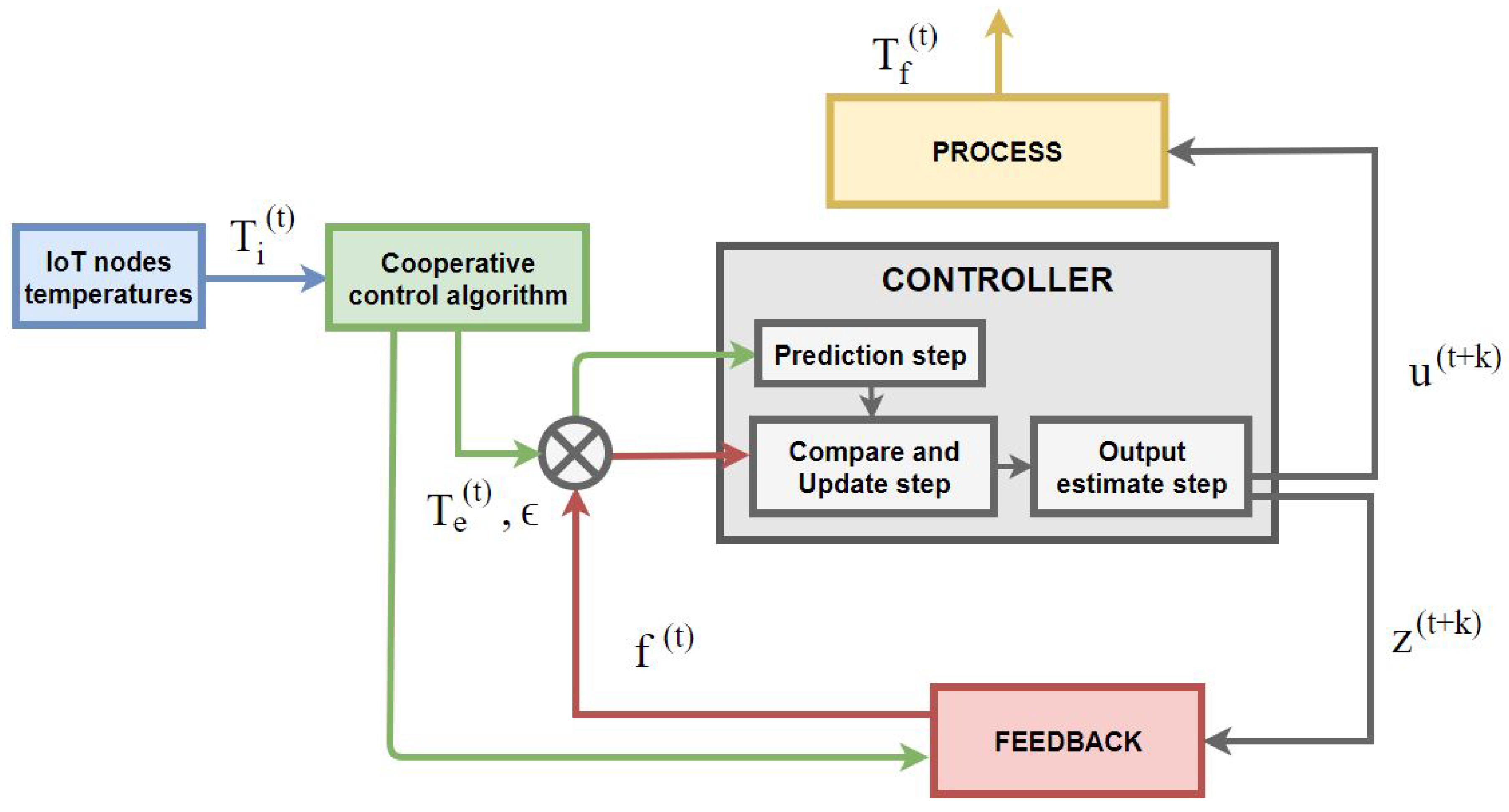
This section presents the control algorithm that we have developed. The control algorithm is a hybrid of two other algorithms: (1) Cooperative control algorithm (Section 2.1). This algorithm receives the data collected by the IoT network and increases the quality of the data by searching and self-correcting false data. The output variables of this algorithm are the input variables of the following algorithm; (2) accuracy state prediction algorithm (Section 2.2). This algorithm implements a predictive maintenance system to make the IoT network more robust. Figure 1 shows the model described in this paper, where $ϵ$ is the measurement error that temperature IoT node are allowed to have. $u^{(t+k)}$ is the controller function, this function detects if an IoT node is faulty or operates correctly at time $t+k$ (i.e., t is the current algorithm step time, while k is a time interval that we want to control. In this way, $t+k$ is the time interval that elapses from the current time t). $z^{(t+k)}$ is the prediction accuracy states function; this function predicts the accuracy state of IoT nodes in the time window $t+k$ (i.e., we know the accuracy state of the IoT nodes at time t, so this function gives us the most probably precision state in time $t+k$). $f^{(t)}$ is the feedback function at time t.

The algorithm proposed in this paper controls the temperature of a smart building. For this purpose, data collected in time t from the IoT network is the input of the algorithm (i.e., $T_i^{(t)}$ in blue block). The cooperative control algorithm forms coalitions of neighboring IoT nodes to detect incorrect data and thus auto-correct temperature. This first part of the proposed algorithm calculates the difference between the collected temperature collected by the IoT network and the optimal output temperature of the cooperative control algorithm. Then, this calculated error (i.e., $T_e^{(t)}$) in time t is sent to the controller as input of the prediction step. The prediction step resolves the Markov strings in continuous-time resulting in the probability that the IoT nodes have the same error that in time t or this error will change. Forecasts of the accuracy state of the IoT nodes are sent to the actuator (i.e., thermostats) to set the process (i.e., smart building) temperature. From the controller, there are two send signals: (1) Since t is the current time in the current loop, assume that k is the time interval to be determined; $z^{(t+k)}$ predicts the accuracy of the IoT nodes at the end of the time interval $t+k$. (2) The second signal that comes out of the controller $u^{(t+k)}$ determines which IoT nodes need to be repaired and which are operating correctly. The process sends the final temperature coming out of the algorithm to the feedback function that compares the prediction of the accuracy states with the new temperature inputs of the algorithm and corrects the error in the predictions for the next step of the algorithm.

2.1. Cooperative Control Algorithm

The cooperative control algorithm is located in the reference input. The cooperative control algorithm requires the data to be in a matrix. The input of this algorithm is the temperature collected by the IoT network of the smart building. This data has a transformation process until it is in the correct form so that the algorithm can process it. The IoT nodes collect the data as follows, IoT node places in: $s_{(i,j)}$ have the following temperature: $t_{s_{(i,j)}}$. The other IoT nodes behave in a similar way. Therefore, the first transformation that data has is to place them in an ordered mesh from point $(1,1)$ to point $(n,n)$ so that each of these points matches the position of the smart nodes. It is easy to create a matrix from the mesh and apply the cooperative control algorithm to it. If we have a mesh with n sensors ordered from $(1,1)$ to $(n,n)$, a matrix shown in Equation (1) is created without loss of generality:

$$T_{n,n}=\left(\begin{array}{ccc}{t}_{s_{1,1}}& \cdots & t_{s_{1,n}}\\ ⋮& \ddots & ⋮\\ t_{s_{n,1}}& \cdots & t_{s_{n,n}}\end{array}\right).$$

(1)

2.1.1. Mathematical Description of the Algorithm

Let $n\ge 2$ be the amount of players in the game, ordered from 1 to n, and let N ={1, 2, ..., n} be the group of players. A coalition, S, is formed to be a subgroup of N, $S\subseteq N$, and the group of the whole coalitions is called by $\mathbb{S}$. A cooperative game in N is a function u (characteristic function of the game) that applies to every coalition $S_i\subseteq \mathbb{S}$ a real number $u(S_i)$. Moreover, one of the conditions is that $u(\varnothing )=0$. In this case, the game will be non-negative (the outputs of the characteristic function are always positive), monotonous (if there are more players in the coalition, the expected characteristic function value does not change), simple and 0-normalized (the players are required to cooperate with one another, as each player will obtain no profit on his own).

In this case, the group of players is the group of organized IoT nodes S and the characteristic function u is denoted as:

$$u:2^n⟶\{0,1\}$$

(2)

so that, for every coalition of nodes, u = 1 or 0 according to a particular coalition can vote or not, respectively (see Equantions (2) and (3)):

$$\mathbb{S}\ni S_i⟶u(S_i)=\{0,1\}\in \mathbb{R},$$

(3)

where $\mathbb{R}$ are the Real numbers.

2.1.2. Cooperative IoT Nodes Coalitions

The potential for IoT nodes to form coalitions will be restricted by their location, i.e., coalitions can only be composed of neighbouring IoT nodes. Let us consider the matrix of the IoT nodes and a pair of IoT nodes $s_{i,j}$ and $s_{k,m}$ will be in the same neighbourhood if and only if:

$$\parallel {(i-k)}^2-{(j-m)}^2\parallel \le 1;$$

(4)

in other words, if every IoT node to which the game is applicable is the centre of a Von Neumann neighborhood, its neighbors are those who are at a Manhattan range (in the matrix) equal to one. In addition, authorized coalitions have to meet the following conditions:

• Coalition of IoT nodes have to be in the same neighborhood as presented in Equation (4).
• Coalitions cannot be formed by a single IoT node.

2.1.3. A Characteristic Function to Find Cooperative Temperatures.

In the suggested game, we want to decide in a democratic way the temperature of the current IoT nodes. To do this, the IoT nodes will create coalitions that will determine the final temperature of the IoT nodes, which will be decided by whether or not they can vote in the election process. From the characteristic function defined in Equation (2), if the value is 1(0), the coalition can vote (not vote) respectively. Assume that $s_i$ is the master IoT node with its related temperature $t_{s_i}$, the characteristic function is built in the following way:

• First, the average temperature of all the IoT node is calculated:

  $$T_{s_i}^k=\frac{1}{V}\sum _i^V{t}_{s_i}.$$

  (5)
  Here, $T_{s_i}^1$ represents the average temperature of the IoT node’ neighbourhood $s_i$ (including it) in the first iteration of the game and V is the amount of neighbours in the coalition.
• The next iteration is to compute an absolute value for the temperature difference between the temperatures of each IoT node and the average temperature:

  $${\overline{T}}_{s_i}^k={\left(\frac{1}{V}\sum _i^V\mid t_{s_i}-T_{s_i}^k{\mid }^2\right)}^{\frac{1}{2}}.$$

  (6)
• Using the differences in temperature values with regards to the average temperature ${\overline{T}}_{s_i}^k$ (see Equation (6)), a confidence interval is created and defined as follows:

  $$I_{s_i}^k=\left(T_{s_i}^k\pm t_{(V-1,\frac{\alpha }{2})}\frac{{\overline{T}}_{s_i}^k}{\sqrt[]{V}}\right).$$

  (7)
  In Equation (7), we use the Student’s t-distribution with a significance level of $\alpha =1\%$.
• In this step, we use a hypothesis test. If the temperature of the sensor lies in the interval $I_{s_i}^k$, it belongs to the voting coalition; otherwise, it is not in the voting coalition. Once the confidence interval is calculated, the algorithm runs the characteristic function of the game $(u^k)$ to find which elements will be in the voting coalition:

  $$u^k(s_1,\dots ,s_n)=\left\{\begin{array}{cc}1,\hfill & \mathrm{if}{t}_{s_i}\in I_{s_i}^k,\hfill \\ 0,\hfill & \mathrm{if}{t}_{s_i}\notin I_{s_i}^k.\hfill \end{array}\right.$$

  (8)
• The characteristic function will repeat this process iteratively (k is the number of the iteration) until all the IoT nodes in that iteration belong to the voting coalition. In the cooperative game theory, the Payoff Vector ($PV$) is the outcome of cooperative actions carried out by coalitions (i.e., the output of applied the characteristic function to the coalitions). At each iteration k, the following $PV$ of the coalition is available $S_j$ (with $1\le j\le n$ where n is the number of sensors in the coalition) in step k ($PV(S_j^k)$):

  $$PV(S_j^k)=(u^k(s_1),\dots ,u^k(s_n))\mathrm{where}\sum _i^n{u}^k(s_i)\le n.$$

  (9)
  The stop condition of the game steps is $PV(S_j^k)$ = $PV(S_j^{k+1})$, at which the algorithm ends. That is, let $PV(S_j^k)=(u^k(s_1),\dots ,u^k(s_n))$ and let $PV(S_j^{k+1})$ = $(u^{k+1}(s_1),\dots ,u^{k+1}(s_n))$. The step process ends when both payoff vectors contain the same elements. This process is shown in the following equation:

  $$\left\{\begin{array}{c}{u}^k(s_1)=u^{k+1}(s_1)\hfill \\ ⋮\hfill \\ u^k(s_n)=u^{k+1}(s_n).\hfill \end{array}\right.$$

  (10)
  Then, the game can find the solution that is shown in the following subsection.

2.1.4. Solution of the Cooperative Game

Once the characteristic function has been applied to all IoT nodes involved in this iteration of the game, a payoff vector is available in iteration k (see Equation (9)). Since the proposed game is cooperative, the solution is a coalition of players that we have called game equilibrium $(GE)$. The $GE$ of the proposed game is defined as the minimal coalition with more than half of the votes cast. Let n be the amount of players in this iteration of the game. The winning coalition has to comply with the following conditions:

• The sum of the elements of the coalition $PV$ must be higher than half plus 1 of the votes cast:

  $$\sum _i^n{u}^k(s_i)\ge \frac{n}{2}+1.$$

  (11)
• The coalition is maximal (i.e., coalition with the greatest number of elements, different from 0, in its payoff vector $PV(S_j^k)$).

Therefore, the solution to the proposed game is the coalition, from among all possible coalitions that are formed at each step k of the game, that satisfies both conditions.

2.1.5. Temperatures of the Winning Coalition

Once the characteristic function finds which is the winning coalition, it is possible to compute the temperature of the main IoT node. Let $\{s_1,\dots ,s_j\}$ be the winning coalition’s IoT node and $\{t_{s_1},\dots ,t_{s_j}\}$ be their related temperature.

The temperature that the game has voted to be the main IoT node’s temperature $(MST)$ is computed as follows:

$$MST=\underset{j\in |{\mathbb{S}}_{winner}|}{max}{\{j·t_{s_i}\}}_{s_{i\in S_{winner}}},$$

(12)

where $\left|\mathbb{S}\right|$ is the amount of elements in the winning coalition. Therefore, the $MST$ will be the maximum temperature that has the highest involved frequency. In the case of a draw, it is resolved by the Lagrange criterion.

2.1.6. Diffuse Convergence

There is a temperature matrix at each game iteration (see Equation (1)). Hence, we define a sequence of arrays ${\{M_n\}}_{n\in \mathbb{N}}$ where the $M_i$ element corresponds to the temperature matrix in step i of the game. Therefore, it can be said that the sequence of matrices is convergent if:

$$\forall ϵ>0,\mathrm{there}\mathrm{is}{i}_0\in \mathbb{N}\mathrm{such}\mathrm{that}|M_{i-1}-M_i|\le ϵ\forall i\in \mathbb{N}.$$

(13)

That is, if the element $m_{n,m}^{i-1}\in M_{i-1}$ and the element $m_{n,m}^i\in M_i$ are set and the convergence criterion is applied, we have:

$$\begin{array}{c}\hfill \forall {ϵ}_{n,m}>0\mathrm{there}\mathrm{is}N\in \mathbb{N}\mathrm{such}\mathrm{that}|m_{n,m}^{i-1}-m_{n,m}^i|\le {ϵ}_{n,m}\\ \hfill \forall i\in \mathbb{N},\forall i\ge i_0\mathrm{and}{m}_{n,m}^{i-1}\in M_{i-1},m_{n,m}^i\in M_i.\end{array}$$

(14)

Therefore, by applying the criterion of convergence in Equation (14) to all the elements, a new matrix is obtained; it calculates the difference in the temperatures obtained in the game’s previous step and those obtained in the current step:

$$\left(\begin{array}{ccc}|m_{1,1}^{i-1}-m_{1,1}^i|& \cdots & |m_{1,m}^{i-1}-m_{1,m}^i|\\ ⋮& \ddots & ⋮\\ |m_{n,1}^{i-1}-m_{n,1}^i|& \cdots & |m_{n,m}^{i-1}-m_{n,m}^i|\end{array}\right).$$

(15)

For the succession of matrices to be convergent, each of the sequences of elements that are formed with the $|m_{n,m}^{i-1}-m_{n,m}^i|$ must be less than the fixed $ϵ>0$. In this work, it is established that $ϵ=0.01$. With the definitions provided above, we are now ready to define the diffuse convergence of the game. The game is diffuse convergent if at least 80 % of the elements of the matrix are convergent; then, the game reaches the equilibrium.

2.2. Accuracy State Prediction Algorithm

In this subsection, we propose a new feedback control algorithm for predictive fault tolerant control to improve the monitoring and control of the IoT networks. Section 2.2.1 presents the accuracy state categories of IoT nodes. The predictive algorithm is based in the continuous-time Markov chains, and, in our model, we compute the solution of this equation in Section 2.2.2. We provide the theoretical solution of the Markov chains (i.e., the transition matrix). Finally, in Section 2.2.3, the elements of the algorithm are shown (i.e, controller, feedback and process).

2.2.1. Initial Accuracy State

Initially, it is necessary to define a scale of accuracy degradation expressed in percentages. This is done according to the data obtained by the algorithm that we had developed in previous research [13]. This scale will be the discussion universe of the random variable $X_n$ that defines the current state of precision of the system related to the error of the sensors. Therefore, the sensors’ possible states are $X_n$ = $\{A=highaccuracy,B=accurate,C=lowaccuracy,F=failure\}$. Below,

Table 1. Accuracy state of sensors.

${\mathit{X}}_{\mathit{n}}$	IoT Nodes Accuracy State	Error (%)
A	High accuracy	e ≤ 10
B	Accurate	10 < e ≤ 20
C	Low accuracy	20 < e ≤ 35
F	Failure	e≥ 35

has the selection made for each variable.

Let $T_i^{(t)}$ be the matrix of initial temperatures collected by the WSN, and let $T_f^{(t)}$ be the final temperatures, obtained after applying the data quality algorithm. Then, the accuracy error matrix of the sensors, according to the data quality algorithm, is given by the following equation:

$$T_e^{(t)}=|T_f^{(t)}-T_i^{(t)}|,$$

(16)

where the coefficients $e_{ij}$ of the matrix $T_e^{(t)}$ are the differences between the initial and final temperature in absolute value for each sensor.

Given the $T_e^{(t)}$ matrix, we now apply the error correction given by the allowed error margin $ϵ$, and adjust the error matrix:

$$T_{ϵ}^{(t)}=|T_e^{(t)}-Id·ϵ|.$$

(17)

Now, let’s centralize these measures to calculate the states of the sensors. To this end, we calculate the average of the elements of the array $m_{ϵ}$ and the maximum of the array $T_{ϵ}^{(t)}$ that we call $ma{x}_{ϵ}$. Therefore, the centralizing measure is defined as:

$$\delta =m_{ϵ}+ma{x}_{ϵ}.$$

(18)

This measure is applied to the matrix $T_{ϵ}^{(t)}$ to calculate the percentages associated with each error and therefore calculate the states of each sensor:

$$T_{\delta }^{(t)}=\left(\begin{array}{ccc}{t}_{1,1}^{\delta }=\frac{(t_{1,1}·100)}{\delta }& \cdots & t_{1,n}^{\delta }=\frac{(t_{1,n}·100)}{\delta }\\ ⋮& \ddots & ⋮\\ t_{n,1}^{\delta }=\frac{(t_{n,1}·100)}{\delta }& \cdots & t_{n,n}^{\delta }=\frac{(t_{n,n}·100)}{\delta }\end{array}\right).$$

(19)

Then, one can define the following function in order to estimate the accuracy state of the sensors in time t. For this purpose, we use the Solution of Kolmogorov’s differential equations to design this function:

$$g^{(t)}:M_{n,n}(\mathbb{R})⟶M_{n,n}(\{X_n\})=T^{g(t)}$$

(20)

defined as follows:

$$g^{(t)}(t_{i,j}^{\delta })=\left\{\begin{array}{ccc}A,\hfill & if& t_{i,j}^{\delta }\le 10\%,\\ B,\hfill & if& 10\%<t_{i,j}^{\delta }\le 20\%,\\ C,\hfill & if& 20\%<t_{i,j}^{\delta }\le 35\%,\\ F,\hfill & if& t_{i,j}^{\delta }\ge 35\%,\end{array}\right.$$

(21)

where $t_{i,j}\in T_{\delta }^{(t)}$, and let $T^{g(t)}$ be the matrix with the accuracy states of the sensors at time t.

2.2.2. Transition Matrix

Let ${\lambda }_A$ be the time the sensor remains in state A (exponential distribution). ${\lambda }_B$ and ${\lambda }_C$ are defined in a similar way. In addition, let ${\xi }_A$ be the time the sensor that remains in state A. Let ${\mu }_A$ (${\mu }_B,{\mu }_C$) be the probability that a sensor in state A (B, C) at time t shifts to state F in the time interval $(t,\Delta t+t)$. Thus, if the sensor was in state A at time $t_i$, the probability of the sensor remaining in state A at time $t_{i+1}$ is given by the following equation:

$$\begin{array}{c}\hfill p_{AA}=P({\xi }_A>t+\Delta t|{\xi }_A>t)=\frac{e^{-{\lambda }_A(t+\Delta t)}}{e^{-{\lambda }_{A}t}}=e^{-{\lambda }_A\Delta t}=1-{\lambda }_A\Delta t+o(\Delta t).\end{array}$$

(22)

Similarly, the probability that a sensor in state A at the beginning will shift to state B is given by the following equation:

$$\begin{array}{cc}\hfill p_{AB}=P({\xi }_B>t+\Delta t|{\xi }_A>t)& =1-((1-{\lambda }_A\Delta t+o(\Delta t))-({\mu }_A\Delta t+o(\Delta t)))\hfill \\ & =({\lambda }_A-{\mu }_A)\Delta t+o(\Delta t).\hfill \end{array}$$

(23)

In this way, we can build the transition matrix between t and $t+\Delta t$, where the coefficients of the transition matrix are the probabilities of the sensors’ switching states (e.g., $p_{AF}$ is the probability that a sensor in state A at the beginning will eventually shift to state F in the interval $(t,\Delta t+t)$).

In this way, the transition matrix $P(t)$ is built:

$$P(t)=\left(\begin{array}{ccc}P({\xi }_A>t+\Delta t|{\xi }_A>t)=p_{AA}& \cdots & p_{AF}\\ ⋮& \ddots & ⋮\\ P({\xi }_A>t+\Delta t|{\xi }_F>t)=p_{FA}& \cdots & p_{FF}\end{array}\right).$$

(24)

2.2.3. Predictive Control Algorithm

Here, we describe how the control algorithm works. This algorithm is used by the sensor control system to monitor and control the accuracy of the sensors. In Figure 1, the set point (green arrow) with the reference inputs contain the following variables: (1) The accuracy error matrix, $T_e$ (see Equation (16)). This matrix has the precision errors of the mesh of sensors. For each step of the algorithm at every time t, this matrix is introduced to update the data of the algorithm. (2) The allowed error $ϵ$. This parameter enters the flow in each of the steps of the algorithm.

Controller

The first action performed by the controller is the prediction step. In this stage of the algorithm, the transition matrix of the developed model is used (see Equation (24)). Let $z^{(t)}:T^{g(t)}⟶z^{(t)}(T^{g(t)})=T^{z(t+k)}$ be the prediction function of accuracy states (i.e., Prediction step) for each time t and let $t+k$ where $k\in \{1,2,\cdots \}$ be the predicted time. Given $t_{i,j}^{\delta }\in T^{\delta }$, the controller function u is defined as follows:

$$\begin{array}{c}\hfill z_{ij}^{(t+k)}(t_{i,j}^g)=max\{{\mathbb{P}}_{t_{i,j}^{g(t+k)}A},{\mathbb{P}}_{t_{i,j}^{g(t+k)}B},{\mathbb{P}}_{t_{i,j}^{g(t+k)}C},{\mathbb{P}}_{t_{i,j}^{g(t+k)}F}\}.\end{array}$$

(25)

Let $z^{(t)}(T^g)=T^{z(t+k)}$ be the matrix of the states of accuracy given by the prediction function. The output of this function is the accuracy state of the sensors at time t.

The next step of the algorithm is to compare the measurements with the feedback function in order to update them. Let $x^{(t)}:T^{z(t)}x{T}^{f(t-k)}⟶x^{(t)}(T^{z(t)})=T^{x(t)}$ be the comparison function defined by the following numerical values $\{A=1,B=2,C=3,F=4\}$ as follows:

$$x^{(t)}(t_{i,j}^{z(t)},t_{i,j}^{f(t-k)})=w_{x_1(t)}{t}_{i,j}^{z(t)}+w_{x_2(t)}{t}_{i,j}^{f(t-k)},$$

(26)

where $w_{x_n(t)}$ with $n\in \{1,2\}$ are the weights given for each of the coordinates of the function x.

Let $y^{(t)}:T^{x(t)}⟶y^{(t)}(T^{x(t)})=T^{y(t)}$ be the update function defined as follows:

$$y^{(t)}(T^{x(t)})=\left\{\begin{array}{ccc}1\hfill & if& 0\le t_{i,j}^{x(t)}\le 1.5,\\ 2\hfill & if& 1.5<t_{i,j}^{x(t)}\le 2.5,\\ 3\hfill & if& 2.5<t_{i,j}^{x(t)}\le 3.5,\\ 4\hfill & if& t_{i,j}^{x(t)}\ge 3.5.\end{array}\right.$$

(27)

The update function refreshes the accuracy states of the prediction function with the results obtained from the comparison function.

Let $u:T^{y(t)}⟶u^{(t)}(T^{y(t)})=T^{u(t)}$ be the controller function (i.e., output estimate step) and let $T^{u(t)}$ be the system controller matrix at time t. Then, this function finds sensors that are in faulty state (F). In this way, the system creates a virtual sensor to maintain system monitoring. In addition, it will send a request to the service staff to replace the malfunctioning sensor. Given $t_{i,j}^{y(t)}\in T^{y(t)}$, u is defined as follows:

$$u(t_{i,j}^{y(t)})=\left\{\begin{array}{ccc}1\hfill & if& t_{i,j}^{y(t)}=F,\\ -1\hfill & if& t_{i,j}^{y(t)}\ne F.\end{array}\right.$$

(28)

Thus, if $u(y^{(t)})=1$, the system creates a virtual sensor in the position $(i,j)$ and requests maintenance.

Feedback

Let $h^{(t)}:T^{g(t)}x{T}^{g(t+k)}x{T}^{z(t+k)}⟶h^{(t)}(T^{z(t+k)})=T^{h(t)}$ be the auxiliary feedback function. Given $k\in \{1,2,\cdots \}$ and the accuracy states in numerical values are $\{A=1,B=2,C=3,F=4\}$, h is defined as follows:

$$\begin{array}{c}\hfill h^{(t)}(t_{i,j}^{g(t)},t_{i,j}^{g(t+k)},t_{i,j}^{z(t+k)})=w_{h_1(t)}{t}_{i,j}^{g(t)}+w_{h_2(t)}{t}_{i,j}^{g(t+k)}+w_{h_3(t)}{t}_{i,j}^{z(t+k)},\end{array}$$

(29)

where $w_{h_n(t)}$ with $n\in \{1,2,3\}$ are the given weights for each of the coordinates of the function h.

Let $f^{(t)}:T^{h(t)}⟶f^{(t)}(T^{h(t)})=T^{f(t)}$ be the feedback function defined as follows:

$$f^{(t)}(T^{h(t)})=\left\{\begin{array}{ccc}A\hfill & if& 0\le t_{i,j}^{h(t)}\le 1.5,\\ B\hfill & if& 1.5<t_{i,j}^{h(t)}\le 2.5,\\ C\hfill & if& 2.5<t_{i,j}^{h(t)}\le 3.5,\\ F\hfill & if& t_{i,j}^{h(t)}\ge 3.5\end{array}\right.$$

(30)

The feedback function returns the accuracy state of the sensor $(i,j)$ back to the flow. In this way, it is verified that the controller is working correctly and that virtual sensors are not created for the repair of sensors that are working properly.

Process

The process matrix $T^{p(t)}$ shows when sensors need maintenance. The process matrix is defined as follows:

$$T^{p(t)}=T^{u(t-1)}+T^{u(t)}.$$

(31)

Thus, when the coefficient of the matrix corresponds to a particular sensor, it means that it has to be replaced $t_{(i,j)}^{p(t)}\ge 0.5\%t_{max}$ time periods with $t_{(i,j)}^{p(t)}\in T^{p(t)}$ (i.e., assuming that $t_{max}=5$ years, then a sensor has to be replaced if $t_{(i,j)}^{p(t)}\ge 9$ days).

Then, the controller function sends a signal to the process which sends back the matrix of final virtual temperatures at time t (i.e., $T_{vf}^{(t)}$). When the controller sends the signal that a sensor is in the state of failure, the process creates a virtual sensor in that position and simulates the temperature so that the monitoring and control of the building does not lose efficiency. Let ${\{T_f^{(t)}\}}_{t\ge 0}$ be the matrix succession with the final temperatures at time t given by the algorithm described in Casado et al. [13]. Moreover, let $V{S}_{i,j}^{(t)}$ be the virtual sensor in the position $(i,j)$ at time t. Then, the temperature of the $t_{i,j}^v$ is provided by the temperature $t_{i,j}\in T_f^{(t)}$.

3. Results

In this section, we present the case study and the results obtained during the experiment. The control algorithm gets data collected by the IoT nodes and auto-corrects the faulty data. Furthermore, in case the controller predicts that an IoT node will be in fault state, it will create a virtual temperature sensor in order to keep the reliability of the IoT network. In this way, the monitoring and control efficiency of the IoT network is improved. This section is organized as follows: In Section 3.1, we provide the solution of the continuous-time Markov chain and its transition matrix $(P(t))$ for every t. Section 3.2 shows the experimental details of the case study (i.e., hardware, temperature collected, etc.). Finally, Section 3.3 presents the results of the application of the control algorithm in the case study and the error decrease in the IoT nodes.

3.1. Case Study Experimental Setup

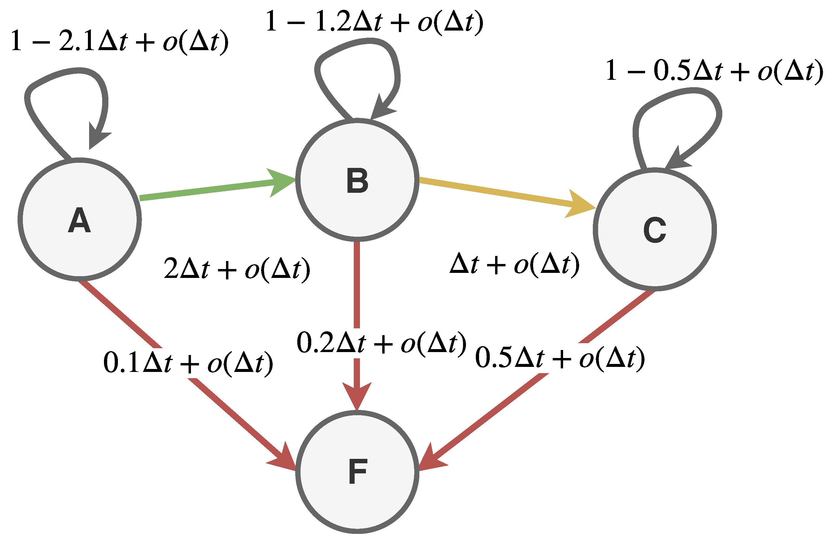
This case study supposes that the IoT nodes (i.e., temperature sensor) can undergo four accuracy states throughout their useful life (A = high accuracy, B = accurate, C = low accuracy, F = failure). The probability that a sensor in state A at instant t shift to state F in the time interval $(t,t+\Delta t)$ is $0.1\Delta t+o(\Delta t)$, if it is in state B it is $0.2\Delta t+o(\Delta t)$ and if it is in state C it is $0.5\Delta t+o(\Delta t)$. In this simulation, we assume that the time during which the sensors remain in state A is an exponential time of $2.1$ in state A and $1.2$ in state B.

From A in a time interval $(t,t+\Delta t),$ the sensor can pass to F with probability $0.1\Delta t+o(\Delta t)$. If $\xi$ is the time the sensor stays at A, you have:

$$\begin{array}{c}\hfill P(\xi >t+\Delta t|\xi >t)=\frac{e^{-2.1(t+\Delta t)}}{e^{-2.1t}}=e^{-2.1\Delta t}=1-2.1\Delta t+o(\Delta t).\end{array}$$

(32)

Therefore, Equation (32) is the probability of remaining in state A at instant $t_{i+1}$ if it was in A at instant $t_i$. Then, the probability of shifting to B between t and $t+\Delta t$ is

$$1-((1-2.1\Delta t+o(\Delta t))-(0.1\Delta t+o(\Delta t)))=2\Delta t+o(\Delta t).$$

(33)

In the successive stages, we finally reach a calculation in which the transition matrix is between t and $t+\Delta t$, as shown in

Table 2. In this simulation, we have assumed that state F is absorbent. That is, for the sensor to move from F to any other state, it needs to be repaired by a maintenance worker.

	A	B	C	F
A	$1-2.1\Delta t+o(\Delta t)$	$2\Delta t+o(\Delta t)$	$o(\Delta t)$	$0.1\Delta t+o(\Delta t)$
B	0	$1-1.2\Delta t+o(\Delta t)$	$\Delta t+o(\Delta t)$	$0.2\Delta t+o(\Delta t)$
C	0	0	$1-0.5\Delta t+o(\Delta t)$	$0.5\Delta t+o(\Delta t)$
F	0	0	0	1

.

Thus, the derivative of the matrix in the zero is:

$$P^{\prime }(0)=\left(\begin{array}{cccc}-2.1& 2& 0& 0.1\\ 0& -1.2& 1& 0.2\\ 0& 0& -0.5& 0.5\\ 0& 0& 0& 0\end{array}\right),$$

(34)

which may be expressed using the Jordan matrix form for the whole period of time t as follows:

$$\begin{array}{c}\hfill P(t)=\left(\begin{array}{cccc}1& 1& 2& 1\\ 1& 0.8& 0.9& 0\\ 1& 0.56& 0& 0\\ 1& 0& 0& 0\end{array}\right)\left(\begin{array}{cccc}1& & & \\ & e^{-0.5t}& & \\ & & e^{-1.2t}& \\ & & & e^{-2.1t}\end{array}\right)\left(\begin{array}{cccc}0& 0& 0& 1\\ 0& 0& \frac{0.9}{0.504}& \frac{-0.9}{0.504}\\ 0& \frac{0.56}{0.504}& \frac{-0.8}{0.504}& \frac{0.24}{0.504}\\ 1& \frac{-1.12}{0.504}& \frac{0.7}{0.504}& \frac{-0.084}{0.504}\end{array}\right).\end{array}$$

(35)

For example, the term $p_{AF}(t)$ represents the probability that a sensor that begins its useful life at stage A functions incorrectly at time t, so:

$$\begin{array}{c}\hfill P(\mathrm{Life}\mathrm{span}\le t)=p_{AF}=1-\frac{0.9}{0.504}{e}^{-0.5t}+\frac{0.48}{0.504}{e}^{-1.2t}-\frac{0.084}{0.504}{e}^{-2.1t}.\end{array}$$

(36)

In Figure 2, the graphical representation of the Markov chain is presented. Probabilities of changes in the accuracy states of the sensors are shown in Table 2. The instance simulation presented in this section demonstrates that sensors in any of the precision states (i.e., A,B,C) can move to the fault state (F)—while from state A it goes to state B, and from state B to state C. This is so, since, in this example, we assume that the sensor from any of its precision states can fail, while we assume that a high accuracy sensor (A) has to go through the precise state (B) before moving to the low accuracy state (C).

Given the Markov chain used for this simulation with transition matrix given by Equation (35), the stationary paths given by the probabilities of change of precision state of the sensors are shown in Figure 2. This figure illustrates the probability that a sensor’s initial accuracy, state A, will shift to a different state in time t. Let’s assume that $t_{max}=5$ years (i.e., lifespan of the sensor is five years), then, at $t=0$, the probability that the sensor remains in state A is 1, while, at $t\ge 0$, the probability that the sensor remains in state A decreases. Thus, the greater the value of t, the greater the probability that a sensor changes to state B, C and F, respectively. For $t⟶\infty$, the accuracy state F of the sensor has a probability of 1 (i.e., the sensor is in failure state) [31].

3.2. General Description of the Experiment

To validate the proposed algorithm, we have selected a smart building. In the moment that the IoT nodes measured the temperature, the actuator (i.e., thermostat) in the selected building showed 23 ${}^{\circ }$C. A grid was applied to locate the IoT nodes on the ground. With the assistance of laser measurements, the IoT nodes were vertically positioned in each section of the building. A total of 25 IoT nodes were deployed.

A combination of the ESP8266 microcontroller in its commercial version “ESP-01” was the type of sensor deployed in the building and a DHT11 temperature and humidity IoT nodes (Figure 2). The sum of the two allows us more versatility in data gathering and adaptation to the case study, as the DHT11 sensor is specifically designed for indoor environments (it has an operating range of 0 ${}^{\circ }$C to 50 ${}^{\circ }$C) according to its datasheet [32]. The microcontroller obtains the data of this IoT nodes through the onewire process and transmits it to the surroundings through Wi-Fi by using HTTP protocols and GET/POST petitions. The ESP-IDF scheduling system supplied by the microcontroller maker was used to schedule the device.

The temperature sensors had been collecting data at 15 minute intervals, for an entire day. For the analysis, we selected the data collected by the sensors in the following time interval 2018-11-02T08:30:00Z and ended on 2018-11-02T21:30:00Z. A particular point in time has been chosen because the game is static and not dynamic (in other words, the game does not handle data in a time period). Below, a mathematical overview of the measured values with the IoT nodes is provided in

Table 3. Statistical table of measurements of the IoT nodes.

Timestamp Start	Total Timestamp	Min Temp	Max Temp	Mean	Standard Deviation
2018-11-02T09:00Z	13:00:00Z	20.1 ${}^{\circ }$C	24.6 ${}^{\circ }$C	22.91 ${}^{\circ }$C	0.71 ${}^{\circ }$C

.

We assume that $t=5$ years, so if we want to find an interval of one day, we have to do some transformation in t. In this experiment, we have considered the next time interval $(t,t+\Delta t)$, a year has 365 days, and 5 years has $(365·5)$ days, so an interval of one day in five years is written as follows: $\Delta t=\frac{1}{365·5}$ (i.e., a day). To validate the model, we applied the accuracy state prediction model to the data collected by the sensors placed in the building.

3.3. Case Study Results

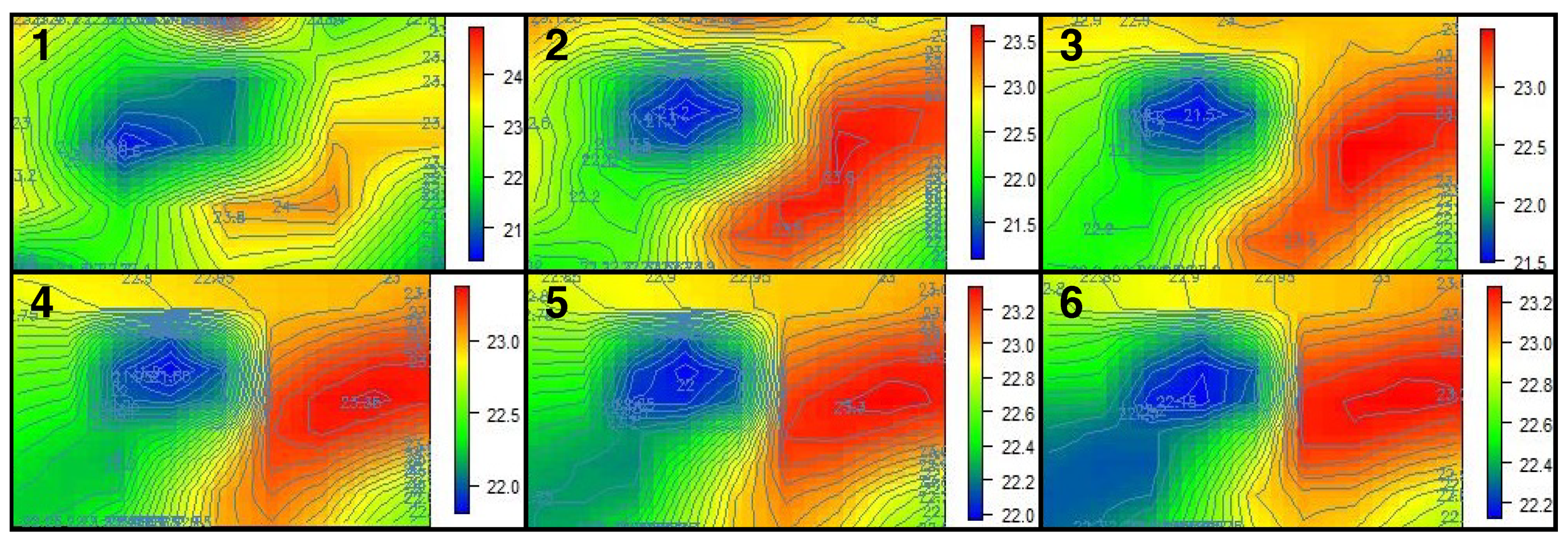
In this case study, we have tested the proposed model to increase the efficiency of monitoring and control of an IoT network. This is achieved by improving the quality of data collected by the IoT nodes and the predicted maintenance of these nodes. In this way, the reliability of the data is increased and the energy efficiency of the smart building is increased. The temperature collected by the IoT nodes is the input of the control algorithm. In Figure 3, the evolution of the temperature can be found from its initial state (i.e., data collected by the IoT nodes) until the control algorithm sends the data to the process to set the regulators that control the temperatures of the building sections. The building temperature is slightly warmer in areas where there are large temperature differences. The control algorithm finds these zones and self-corrects if necessary these temperatures to reach the equilibrium in which the temperatures are consistent in the whole building.

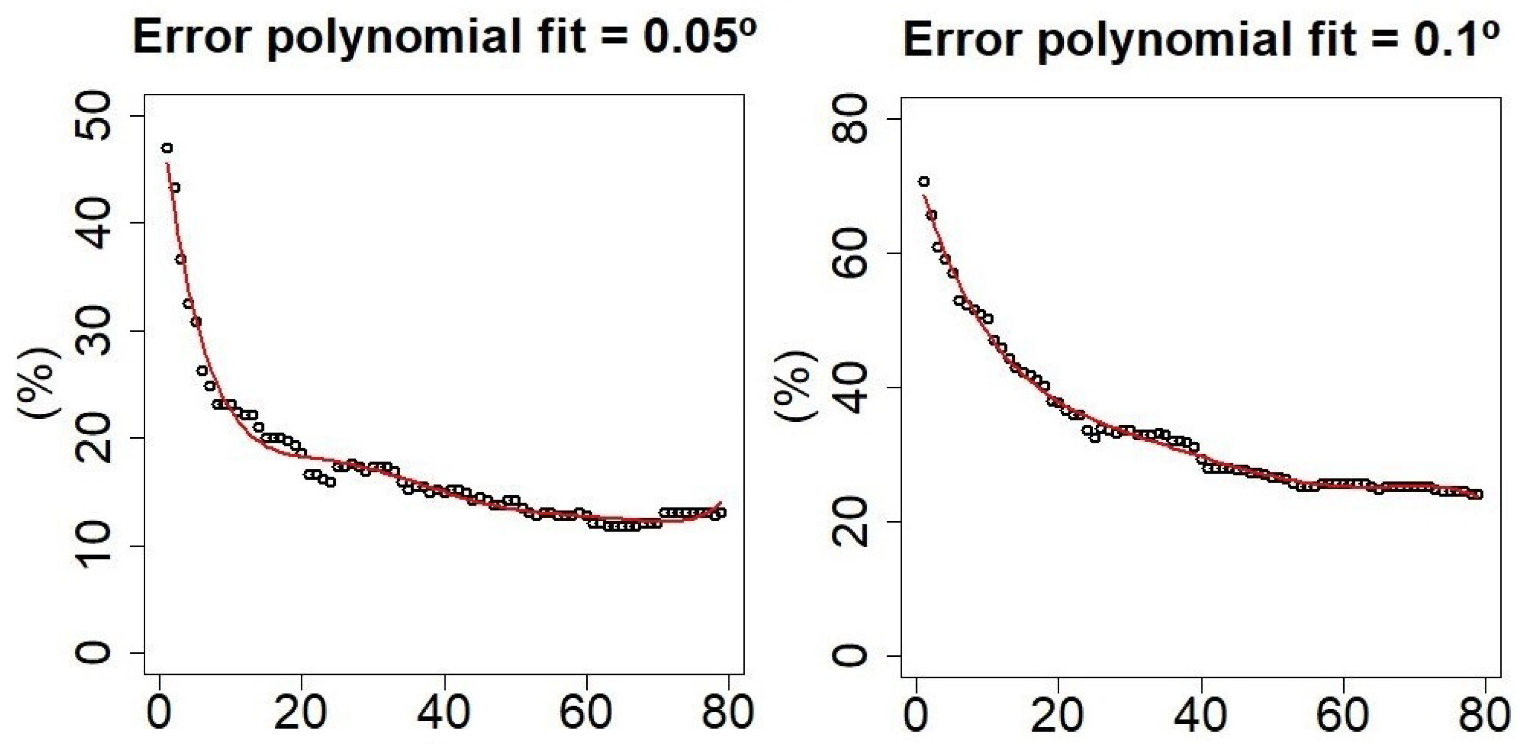
The suggested algorithm performs an efficient transformation in the ETL system. We can implement our approach as a process step included in the ETL system for the creation of new temperature data, which are self-corrected and ready-to-use. A major part of the thermal noise caused by the data arriving from the IoT node is removed (noise is generated when the IoT node is faulty or non-accurate). Figure 4 provides the amount of IoT nodes (in percents) containing thermal noise for every step of the game. It can be remarked that, when changing the accuracy of the IoT nodes from $0.05{}^{\circ }$C to $0.1{}^{\circ }$C, the results achieved are quite distinct.

However, if it changes to $0.05{}^{\circ }$C, 45% of the IoT nodes had thermal noise, and, in a few (<10) steps, the noise was decreased to less than 15%. When the relative permitted error was incremented, the percentages of IoT nodes that had a bit of thermal noise also incremented. For instance, with $0.1{}^{\circ }$C of relative error, 70% of the IoT nodes had thermal noise and as the step increment was decreased below 25 percent. However, at a certain point, the noise began to freeze. These IoT nodes will keep having some noise for the selected error (

Table 4. Table showing the possible errors and % of noise both during and after applying the game.

Allowed Error (${}^{\circ }$ Celsius)	IoT Nodes with Noise at the Beginning (%)	IoT Nodes with Noise at the End (%)
0.05	47.06	13.25
0.1	70.59	24.22

).

There are also two useful implementations of our current approach: $(1)$ Identifying the IoT nodes that supply incorrect data and setting up the new IoT node by inserting them in the IoT network; $(2)$ Smart detecting of incorrect data in an IoT network is a major issue, as it allows fault tolerant control of the IoT network and a high quality of data. Furthermore, predictive maintenance allows the good operation of the IoT network. As faulty IoT nodes are detected, the maintenance cost is significantly decreased, as the service technician can focus only on faulty nodes.

4. Conclusions

This paper has addressed the problem of fault tolerant control of IoT nodes in continuous-time NCSs. The feasibility of the proposed approach was verified with a case study in which the closed-loop system was modeled as a continuous-time feedback system with the continuos-time Markov chains to improve the quality of the data collected by the IoT nodes. Through a newly constructed feedback control-based algorithm, an improved control system has been created. It allows for deriving a smart building’s maximum allowable energy efficiency such that the resulting closed-loop system improves the control of an IoT network. A numerical case study illustrates the efficiency of our model in Section 3. Figure 3 shows a graphic representation of the evolution of the temperatures and how the fault tolerant control algorithm works. In this figure, one can find how the incorrect data are self-corrected by the control algorithm, improving the monitors and controls of the IoT network. In addition, in Figure 4, we present the percentage of IoT nodes that are collecting incorrect data and how the control algorithm decreases the amount of malfunction IoT nodes. This claim is also supported by Table 4. In it, you can find that, after applying the control algorithm, the amount of malfunctioning IoT nodes is greatly reduced. However, in many real scenarios, the ability to detect an imprecise or malfunctioning IoT node from a hot (cold) spot is limited. In a future work, we will try to solve this problem with artificial intelligence.

References

- Hespanha, J.P.; Naghshtabrizi, P.; Xu, Y. A survey of recent results in networked control systems. Proc. IEEE 2007, 95, 138–162. [Google Scholar] [CrossRef]
- Mo, Y.; Garone, E.; Casavola, A.; Sinopoli, B. False data injection attacks against state estimation in wireless sensor networks. In Proceedings of the 2010 49th IEEE Conference on Decision and Control (CDC), Atlanta, GA, USA, 15–17 December 2010; pp. 5967–5972. [Google Scholar]
- Amato, F.; Ariola, M.; Cosentino, C. Finite-time stabilization via dynamic output feedback. Automatica 2006, 42, 337–342. [Google Scholar] [CrossRef]
- Amato, F.; Ariola, M.; Cosentino, C. Finite-time control of discrete-time linear systems: Analysis and design conditions. Automatica 2010, 46, 919–924. [Google Scholar] [CrossRef]
- Polyakov, A.; Efimov, D.; Perruquetti, W. Robust stabilization of MIMO systems in finite/fixed time. Int. J. Robust Nonlinear Control 2016, 26, 69–90. [Google Scholar] [CrossRef]
- Korobov, V.I.; Pavlichkov, S.S.; Schmidt, W.H. Global positional synthesis and stabilization in finite time of MIMO generalized triangular systems by means of the controllability function method. J. Math. Sci. 2013, 189, 795–804. [Google Scholar] [CrossRef]
- Hui, Q.; Haddad, W.M.; Bhat, S.P. Finite-time semistability and consensus for nonlinear dynamical networks. IEEE Trans. Autom. Control 2008, 53, 1887–1900. [Google Scholar] [CrossRef]
- Khoo, S.; Xie, L.; Zhao, S.; Man, Z. Multi-surface sliding control for fast finite-time leader–follower consensus with high order SISO uncertain nonlinear agents. Int. J. Robust Nonlinear Control 2014, 24, 2388–2404. [Google Scholar] [CrossRef]
- Soares, J.; Ghazvini, M.A.F.; Borges, N.; Vale, Z. A stochastic model for energy resources management considering demand response in smart grids. Electr. Power Syst. Res. 2017, 143, 599–610. [Google Scholar] [CrossRef]
- Li, Y.; Tong, S.; Li, T. Composite adaptive fuzzy output feedback control design for uncertain nonlinear strict-feedback systems with input saturation. IEEE Trans. Cybern. 2015, 45, 2299–2308. [Google Scholar] [CrossRef]
- Li, Y.X.; Yang, G.H. Event-triggered adaptive backstepping control for parametric strict-feedback nonlinear systems. Int. J. Robust Nonlinear Control 2018, 28, 976–1000. [Google Scholar] [CrossRef]
- Pipino, L.L.; Lee, Y.W.; Wang, R.Y. Data quality assessment. Commun. ACM 2002, 45, 211–218. [Google Scholar] [CrossRef]
- Casado-Vara, R.; Prieto-Castrillo, F.; Corchado, J.M. A game theory approach for cooperative control to improve data quality and false data detection in WSN. Int. J. Robust Nonlinear Control 2018, 28, 5087–5102. [Google Scholar] [CrossRef]
- Wang, R.Y. A product perspective on total data quality management. Commun. ACM 1998, 41, 58–65. [Google Scholar] [CrossRef]
- Liu, K.; Seuret, A.; Fridman, E.; Xia, Y. Improved stability conditions for discrete-time systems under dynamic network protocols. Int. J. Robust Nonlinear Control 2018, 28, 4479–4499. [Google Scholar] [CrossRef]
- Zhang, X.; Lin, Y. Adaptive output feedback tracking for a class of nonlinear systems. Automatica 2012, 48, 2372–2376. [Google Scholar] [CrossRef]
- Lezama, F.; Soares, J.; Hernandez-Leal, P.; Kaisers, M.; Pinto, T.; do Vale, Z.M.A. Local energy markets: Paving the path towards fully Transactive energy systems. IEEE Trans. Power Syst. 2018. [Google Scholar] [CrossRef]
- Rodriguez-Fernandez, J.; Pinto, T.; Silva, F.; Praça, I.; Vale, Z.; Corchado, J.M. Context aware q-learning-based model for decision support in the negotiation of energy contracts. Int. J. Electr. Power Energy Syst. 2019, 104, 489–501. [Google Scholar] [CrossRef]
- Faria, P.; Spínola, J.; Vale, Z. Reschedule of Distributed Energy Resources by an Aggregator for Market Participation. Energies 2018, 11, 713. [Google Scholar] [CrossRef]
- Fotouhi Ghazvini, M.A.; Soares, J.; Morais, H.; Castro, R.; Vale, Z. Dynamic Pricing for Demand Response Considering Market Price Uncertainty. Energies 2017, 10, 1245. [Google Scholar] [CrossRef]
- Silva, F.; Teixeira, B.; Pinto, T.; Santos, G.; Vale, Z.; Praça, I. Generation of realistic scenarios for multi-agent simulation of electricity markets. Energy 2016, 116, 128–139. [Google Scholar] [CrossRef]
- Santos, G.; Pinto, T.; Praça, I.; Vale, Z. An interoperable approach for energy systems simulation: Electricity market participation ontologies. Energies 2016, 9, 878. [Google Scholar] [CrossRef]
- Zhang, X.; Lin, Y. Adaptive output feedback control for a class of large-scale nonlinear time-delay systems. Automatica 2015, 52, 87–94. [Google Scholar] [CrossRef]
- Zhang, J.X.; Yang, G.H. Fault-tolerant leader-follower formation control of marine surface vessels with unknown dynamics and actuator faults. Int. J. Robust Nonlinear Control 2018, 28, 4188–4208. [Google Scholar] [CrossRef]
- Ghazvini, M.A.F.; Soares, J.; Abrishambaf, O.; Castro, R.; Vale, Z. Demand response implementation in smart households. Energy Build. 2017, 143, 129–148. [Google Scholar] [CrossRef]
- Wang, H.; Liu, K.; Liu, X.; Chen, B.; Lin, C. Neural-based adaptive output-feedback control for a class of nonstrict-feedback stochastic nonlinear systems. IEEE Trans. Cybern. 2015, 45, 1977–1987. [Google Scholar] [CrossRef] [PubMed]
- Casado-Vara, R.; González-Briones, A.; Prieto, J.; Corchado, J.M. Smart Contract for Monitoring and Control of Logistics Activities: Pharmaceutical Utilities Case Study. In Proceedings of the 13th International Conference on Soft Computing Models in Industrial and Environmental Applications, San Sebastian, Spain, 6–8 June 2018; Springer: Cham, Germany, 2018; pp. 509–517. [Google Scholar]
- Casado-Vara, R.; Prieto, J.; De la Prieta, F.; Corchado, J.M. How blockchain improves the supply chain: Case study alimentary supply chain. Procedia Comput. Sci. 2018, 134, 393–398. [Google Scholar] [CrossRef]
- Casado-Vara, R.; Prieto, J.; Corchado, J.M. How Blockchain Could Improve Fraud Detection in Power Distribution Grid. In Proceedings of the 13th International Conference on Soft Computing Models in Industrial and Environmental Applications, San Sebastian, Spain, 6–8 June 2018; Springer: Cham, Germany, 2018; pp. 67–76. [Google Scholar]
- Casado-Vara, R.; de la Prieta, F.; Prieto, J.; Corchado, J.M. Blockchain framework for IoT data quality via edge computing. In Proceedings of the 1st Workshop on Blockchain-enabled Networked Sensor Systems, Shenzhen, China, 4 November 2018; pp. 19–24. [Google Scholar]
- Mailund, T. Continuous-Time Markov Chains. In Domain-Specific Languages in R; Apress: Berkeley, CA, USA, 2018; pp. 167–182. [Google Scholar]
- DHT11 datasheet. Available online: http://www.micropik.com/PDF/dht11.pdf (accessed on 6 December 2018).
Figure 1.
This algorithm improves the fault tolerance of the IoT network via the designed control algorithm in the time interval , where k is the interval of time that we want to control.
Figure 2.
Graphical representation of the Markov chain of the solution of the Kolmogorov differential equations of the proposed simulation.
Figure 3.
Graphic representation of the matrix of initial temperatures, the evolution of the temperature and the final temperatures in this case study. In Figure 3 (1) can be found the temperatures collected by the IoT nodes. In addition, the measurements that the control algorithm will find as false data can be found in the same figure. Also, the evolution of the controlled temperature is shown in Figure 3 (2)–(5). Final temperatures after the control algorithm is executed are shown in Figure 3 (6).
Figure 4.
Board with thermal noise reduction in the progression of the algorithm with several confidence intervals from 0.05 C to 0.1 C. In the display board, the noise of the % in the temperature matrix is shown opposite the amount of steps. For every one of them, the permitted error range for the temperature collected by the IoT nodes is variable. As the allowable error range is increased, the thermal noise in the temperature matrix also is increased.