Zoning Evaluation for Voltage Optimization in Distribution Networks with Distributed Energy Resources

Abstract

This paper deals with the problem of the voltage profile optimization in a distribution system including distributed energy resources. Adopting a centralized approach, the voltage optimization is a non-linear programming problem with large number of variables requiring a continuous remote monitoring and data transmission from/to loads and distributed energy resources. In this study, a recently-proposed Jacobian-based linear method is used to model the steady-state operation of the distribution network and to divide the network into voltage control zones so as to reformulate the centralized optimization as a quadratic programming of reduced dimension. New clustering methods for the voltage control zone definition are proposed to consider the dependence of the nodal voltages on both active and reactive powers. Zoning methodologies are firstly tested on a 24-nodes low voltage network and, then, applied to the voltage optimization problem with the aim of analyzing the impact of the R/X ratios on the zone evaluation and on the voltage optimization solution.

1. Introduction

In the normal operation of modern distribution systems, variations of active and reactive powers absorbed and/or injected by controllable loads, distributed generators (DGs), and energy storage systems (ESSs) as well as changes in network topology can cause violation of the nodal voltage limits, fixed to $\pm 10$% of the rated voltage of the grid.

Presently, the utility-side voltage regulation cannot adequately respond to the voltage variations. In fact, the conventional Volt/Var control devices (i.e., on-load tap changer of the transformer in the HV/MV substations, step voltage regulators and capacitor banks) have slow response time and can negatively interfere with distributed energy resources (DERs) (i.e., DGs, ESSs including electrical vehicles, and smart loads), deteriorating voltage regulation. To keep the nodal voltages within the admissible limits, new flexible voltage control strategies have to be developed, involving both conventional devices and DERs [1].

The recently-proposed architectures for voltage regulation can be classified into local control and communication-based control according to whether the use of communication infrastructures is not or is required. The second category can be further split into: centralized, distributed and decentralized control architectures [2].

In a local control, the controllers of both DERs and conventional Volt/Var devices use measurements at the point of common coupling (PCC) to individually elaborate and actuate a control action without requiring any information exchange. The result is a globally non-optimal control solution. Undoubtedly, this is the lowest-cost solution to start involving DERs in the voltage control of existing distribution networks. Unfortunately, the absence of coordination may introduce technical problems related to the interaction among controllers or even system instability [3,4].

In a centralized control, a central control unit, located at the substation level, firstly solves a system voltage optimization/control problem by receiving measurements from all the nodes of the network; then, it sends the optimal set-points back to the local controller of both DERs and conventional Volt/Var devices. This approach yields the optimal solution but its implementation is very expensive requiring a large communication infrastructure with adequate bandwidth to exchange information quickly and accurately [5,6,7,8].

In a distributed control, the controllers of both DERs and conventional Volt/Var devices use measurements at PCC to achieve local voltage regulation as in a local control but they also exchange information with the controllers of the neighboring nodes. This approach aims at overcoming the technical problems of the local control while limiting the investments for the communication infrastructure [9,10].

In a decentralized approach, the distribution system is usually partitioned into voltage control zones (VCZs). Each VCZ contains nodes weakly coupled with the nodes belonging to other VCZs from an electrical point of view; in the ‘electric center’ of a VCZ is placed the pilot node (PN), whose voltage variation best represents the variation of the voltage in the VCZ. In each VCZ a centralized control is present whereas the coordination is obtained by a distributed control among the PNs. This approach guarantees the optimal solution for each VCZ and it requires a communication infrastructure lighter than the centralized control [11,12].

The division of the network in VCZs require the definition of an electrical distance, a clustering criterion and, in some case, a clustering quality index [13]. In literature, various measures of the electrical distance have been proposed, based on geographical distance, line impedance, voltage sensitivity coefficients [14] and the most commonly used involves the sensitivity of the nodal voltages to the reactive power injections [13,15,16,17,18,19,20,21]. Such an approach is typically adopted for the secondary voltage control in transmission systems. Unfortunately, in distribution systems nodal voltages depends on both active and reactive power injections due to the high R/X ratio of the grid. To face this problem, in [22] electrical distances are evaluated taking into account the dependence of the nodal voltages to the active powers. In [11,12] both the sensitivities of the nodal voltages to active and reactive powers injected by DERs are considered and used for the definition of a weighted linear electrical distance. In [23] a modified electrical distance is proposed combining the voltage sensitivities in [11,12] with the conventional definition of electrical distances derived from the line impedance measure. Moreover, there are also many methods for grouping the nodes with similar electrical distances in VCZs, such as hierarchical clustering [11,13,16,17], K-means clustering [18], genetic algorithms [19,24].

In this paper, extending and improving the approach proposed in [14], a partition of the distribution network in VCZs that account for the sensitivities of the nodal voltages to active and reactive powers is firstly proposed and then applied to optimize the voltage profiles of the distribution feeders with DERs. In particular, using the sensitivity coefficients derived from the linear method for the steady-state analysis of the distribution system in [25,26], various definitions of the electrical distance are proposed in this paper, which consider separately or simultaneously the dependence of the nodal voltages on active and reactive power injections, independently from the number and position of the DERs. Successively, the hierarchical clustering algorithm in [16] is adopted and extended to adequately work also with two electrical distances defined for each node. Then, adopting the centralized approach as in [15], the zoning methodologies are applied to optimize the voltage profile of the distribution systems with DERs so as to guarantee a solution close to the optimal one and to reduce the requirements for the monitoring and communication infrastructures. Finally, the influence of different R/X ratios on the proposed zoning methodologies as well as on the voltage optimization problem is analyzed in a case study.

Differently from [11,12,22,23], in this paper various electrical distance measures have been proposed accounting for active and reactive power sensitivities, which are identified on the basis of the structural characteristics of the power grid thanks to the linear model in [25,26]. Compared to [15], in this paper: (i.) the sensitivities of the nodal voltages to not only reactive but also active powers are considered; (ii.) the hierarchical clustering algorithm is extended to obtain aggregation based on active and reactive powers; (iii.) the centralized voltage optimization problem includes DERs with controllable active and reactive powers; (iv.) the impact of the R/X ratios on the VCZ evaluation and on the voltage optimization solution is analyzed and general considerations are derived.

The paper is organized as follows: the linear method for the steady-state operation of the distribution system is briefly recalled in Section 2. Section 3 presents the proposed zoning methodologies and includes Appendix A and Appendix B containing the extensions of the hierarchical clustering algorithms. In Section 4 the application of the zoning methodology to the voltage optimization problem is reported. Referring to a 24-nodes distribution system, in Section 5 various network partitioning options are tested and, then, applied to the centralized voltage optimization problem.

2. Brief Recalls of the Linear Method

A Jacobian-based method for the steady-state analysis of radially-operated distribution systems with DERs has recently been presented in [25,26]. Starting from an initial operating point, it provides the closed-form analytical expressions of the sensitivity coefficients that linearly relate the variations of the electrical variables characterizing each node of a feeder to the variations of the powers injected by all the DERs connected to the grid.

Referring all the variations with respect to the initial operating point, the steady-state linear model of a radial distribution network with $N$ nodes including DERs is expressed as:

$${\left(\Delta P_i,\Delta Q_i,\Delta V_i^2\right)}^T=\sum _{k\in K_{der}}\left(\begin{array}{cc}\frac{\partial P_i}{\partial P_k^{der}}& \frac{\partial P_i}{\partial Q_k^{der}}\\ \frac{\partial Q_i}{\partial P_k^{der}}& \frac{\partial Q_i}{\partial Q_k^{der}}\\ \frac{\partial V_i^2}{\partial P_k^{der}}& \frac{\partial V_i^2}{\partial Q_k^{der}}\end{array}\right){\left(\Delta P_k^{der},\Delta Q_k^{der}\right)}^T\hspace{1em}i=1,\dots ,N,$$

(1)

where:

• $\Delta P_i$ and $\Delta Q_i$ are the variations of, respectively, the active and the reactive powers out-flowing the $i$-th node of the grid;
• $\Delta V_i^2$ is the variation of the squared nodal voltage at the $i$-th node of the grid;
• $K_{der}$ is a subset of $\left\{1,\dots , N\right\}$ including only the nodes of the network with DERs;
• $\Delta P_k^{der}\mathrm{and}\Delta Q_k^{der}$ are the variations of, respectively, the active and reactive powers injected by a DER at the $k$-th node of the grid.

The sensitivity coefficients in (1), relating the electrical variables at the $i$-th node to the power injections of the DER connected at the $k$-th node, can be collected in the $\left(3\times 2\right)$ matrices ${\mathit{T}}_i\left(k\right)$:

$${\mathit{T}}_i\left(k\right)\triangleq \left(\begin{array}{cc}\frac{\partial P_i}{\partial P_k^{der}}& \frac{\partial P_i}{\partial Q_k^{der}}\\ \frac{\partial Q_i}{\partial P_k^{der}}& \frac{\partial Q_i}{\partial Q_k^{der}}\\ \frac{\partial V_i^2}{\partial P_k^{der}}& \frac{\partial V_i^2}{\partial Q_k^{der}}\end{array}\right)\hspace{1em}i=1,\dots ,N\hspace{1em}k\in K_{der},$$

(2)

so that:

$${\left(\Delta P_i,\Delta Q_i,\Delta V_i^2\right)}^T={\sum }_{k\in K_{der}}{\mathit{T}}_i\left(k\right){\left(\Delta P_k^{der},\Delta Q_k^{der}\right)}^T\hspace{1em}i=1,\dots ,N.$$

(3)

In Equations (1) and (3) DERs are assumed to be equipped with P-Q control; the extension of the model to the distribution network including DERs with different types of controls is detailed in [15]. It is worth noting that the adoption of the new variable $\Delta V_i^2$ (in place of $\Delta V_i$) permits to limit the approximation caused by the linearization of the power flow equations with respect to other Jacobian-based methods.

3. Zoning Methodologies

The aim of a zoning methodology is to obtain a simplified representation of the distribution network suitable for voltage control. Basically, the problem involves four steps [13]:

• Defining an electrical distance among the nodes of the network;
• Grouping the nodes into VCZs;
• Identifying a PN in each VCZ;
• Determining the optimum number of VCZs.

The electrical distance among the nodes as well as the topology of the network are important to deeply investigate the structure of a power grid. The electrical distance is a measure of the electrical connectedness among the nodes. Various measures of the electrical distance have been proposed [14] but the most commonly used involves the Jacobian matrix of the load flow equations and its inverse, named sensitivity matrix. Adopting and extending the approach outlined in [15], various definitions of the electrical distance are proposed in this paper, based on the sensitivity coefficients derived from the linear model recalled in Section 2 with respect to both active and reactive powers.

After the first step, nodes with similar electrical distances are grouped to form a VCZ; those nodes in turn result to be weakly coupled from an electrical point of view with the nodes belonging to other VCZs. In other words, the problem of grouping the nodes in VCZs is transformed into a clustering problem in the space of the electrical distance. Clustering can be achieved by various algorithms [20] but one of the most commonly used is the hierarchical algorithm [11,13,16,17], which is adopted in this paper and extended to account for various electrical distances.

Once the VCZs are available from the second step, for each VCZ a PN is identified. The PN is chosen as the node whose voltage variation best represents the voltage variations of all the nodes in the VCZ. The identification of the PN of a VCZ is based on an extension of the algorithm in [20] that evaluates the proximity of each node to all the other nodes belonging to the same VCZ.

Finally, in the last step, the best number of VCZs is chosen. To this aim, an index that represents the goodness of the clustering results must be used; in this paper, the Silhouette index [27,28] is used because it is the most adequate for hierarchical algorithms.

3.1. Electrical Distances

In a radial distribution network with a DER connected at the $k$-th node, the square nodal voltage at the $i$-th node varies for the changes of both DER active and reactive power injections according to:

$$\Delta V_i^2=\frac{\partial V_i^2}{\partial P_k^{der}}\Delta P_k^{der}+\frac{\partial V_i^2}{\partial Q_k^{der}}\Delta Q_k^{der} i=1, \dots , N$$

(4)

The voltage sensitivity coefficients to the DER active and reactive powers can be evaluated by extracting the third row of ${\mathit{T}}_i\left(k\right)$ in (2):

$$\frac{\partial V_i^2}{\partial P_k^{der}}=t_{i_{3,1}}\left(k\right) i=1, \dots , N,$$

(5)

$$\frac{\partial V_i^2}{\partial P_k^{der}}=t_{i_{3,2}}\left(k\right) i=1, \dots , N.$$

(6)

Assuming to connect a DER in each node of the network (i.e., $k=1, \dots , N$), the voltage sensitivity coefficients to the DER active and reactive powers can be collected in two ($N\times N$) voltage sensitivity matrices, respectively ${\mathit{\Gamma }}_P$ and ${\mathit{\Gamma }}_Q$, whose generic elements are:

$${\Gamma }_{P_{i,k}}=t_{i_{3,1}}\left(k\right) i,k=1, \dots , N,$$

(7)

$${\Gamma }_{Q_{i,k}}=t_{i_{3,2}}\left(k\right) i,k=1, \dots , N.$$

(8)

The electrical distances among the nodes of the network can be evaluated by using three sensitivity measures described in the following, namely:

• Sensitivity to the only active power;
• Sensitivity to the only reactive power;
• Sensitivity to both active and reactive powers.

3.1.1. Sensitivities to Active Powers

Considering only the impact of the active power, the variation of the square nodal voltage at the $i$-th node to the change of the DER active power at the $k$-th node is equal to:

$$\Delta V_i^2={\Gamma }_{P_{i,k}}\Delta P_k^{der} i,k=1, \dots , N.$$

(9)

Similarly, the variation of the square nodal voltage at the $k$-th node to the change of the DER active power at the $k$-th node is equal to:

$$\Delta V_k^2={\Gamma }_{P_{i,k}}\Delta P_k^{der} i,k=1, \dots , N.$$

(10)

Dividing Equation (9) by Equation (10), the variation of the voltage at the i-th node to the change of the DER active power at the k-th node can be rewritten in terms of ‘voltage attenuation’ of the voltage variation between the nodes i and k caused by an active power variation in k as:

$$\Delta V_i^2=\left(\frac{{\Gamma }_{P_{i,k}}}{{\Gamma }_{P_{k,k}}}\right)\Delta V_k^2 i,k=1, \dots , N.$$

(11)

The concept of electrical distance used in this paper is presented in [16]. To define a measurement with symmetrical property, the product of the voltage attenuations between nodes $i$ and $k$ and between nodes $k$ and $i$ is considered. Moreover, to obtain a null distance between a node and itself the logarithmic function is used. The electrical distance between the nodes i and $k$, $D_{P_{i,k}}$, is then defined as:

$$D_{P_{i,k}}=D_{P_{k,i}}=-\log \left(\frac{{\Gamma }_{P_{i,k}}}{{\Gamma }_{P_{k,k}}}\frac{{\Gamma }_{P_{k,i}}}{{\Gamma }_{P_{i,i}}}\right) i,k=1, \dots , N.$$

(12)

The values of the electrical distances are usually normalized according to:

$$D_{P_{i,k}}=\frac{D_{P_{i,k}}}{\underset{i,k}{\max }{D}_{P_{i,k}}} i,k=1, \dots , N,$$

(13)

and, then, collected in the $\left(N\times N\right)$ electrical distance matrix ${\mathit{D}}_{\mathit{P}}$; such a matrix represents a network divided in $N$ VCZs.

3.1.2. Sensitivities to the Reactive Powers

Considering only the impact of the reactive power, the electrical distance between the nodes i and k, $D_{Q_{i,k}}$ is defined in a similar way as for the active powers, see Equation (12):

$$D_{Q_{i,k}}=D_{Q_{k,i}}=-\log \left(\frac{{\Gamma }_{Q_{i,k}}}{{\Gamma }_{Q_{k,k}}}\frac{{\Gamma }_{Q_{k,i}}}{{\Gamma }_{Q_{i,i}}}\right) i,k=1, \dots , N.$$

(14)

and the normalized measures are collected in the $\left(N\times N\right)$ electrical distance matrix ${\mathit{D}}_Q$.

3.1.3. Sensitivities to Active and Reactive Powers

Considering the impact of both active and reactive powers on the voltage amplitudes, the electrical distance between the nodes i and k can be defined using the mathematical concept of Manhattan distance as:

$$D_{{PQ}_{i,k}}^1=\left|-\log \left(\frac{{\Gamma }_{P_{i,k}}}{{\Gamma }_{P_{k,k}}}\frac{{\Gamma }_{P_{k,i}}}{{\Gamma }_{P_{i,i}}}\right)\right|+\left|-\log \left(\frac{{\Gamma }_{Q_{i,k}}}{{\Gamma }_{Q_{k,k}}}\frac{{\Gamma }_{Q_{k,i}}}{{\Gamma }_{Q_{i,i}}}\right)\right|\hspace{1em}\hspace{1em}i,k=1,\dots ,N.$$

(15)

or adopting the Euclidean distance:

$$D_{{PQ}_{i,k}}^2=\sqrt{{\left|-\log \left(\frac{{\Gamma }_{P_{i,k}}}{{\Gamma }_{P_{k,k}}}\frac{{\Gamma }_{P_{k,i}}}{{\Gamma }_{P_{i,i}}}\right)\right|}^2+{\left|-\log \left(\frac{{\Gamma }_{Q_{i,k}}}{{\Gamma }_{Q_{k,k}}}\frac{{\Gamma }_{Q_{k,i}}}{{\Gamma }_{Q_{i,i}}}\right)\right|}^2}\hspace{1em}\hspace{1em}i,k=1,\dots ,N.$$

(16)

After the normalization $D_{P{Q}_{i,k}}^1$ and $D_{P{Q}_{i,k}}^2$ are collected into the $\left(N\times N\right)$ electrical distance matrices ${\mathit{D}}_{PQ}^1$ and ${\mathit{D}}_{PQ}^2$, respectively.

3.2. Voltage Control Zones

The aggregation of the nodes in VCZs is performed by using the previously-defined electrical distances. The related matrices (${\mathit{D}}_P$, ${\mathit{D}}_Q$, ${\mathit{D}}_{PQ}^1$ and ${\mathit{D}}_{PQ}^2$) represent a starting point, that is a network composed of $N$ VCZs, each VCZ coinciding with a node. The aim is to aggregate the N nodes into VCZs yielding the set $VCZ=\left\{VC{Z}_1,\dots ,VC{Z}_{N_{vcz}}\right\}$ composed by the $N_{vcz}$ subsets $VC{Z}_h$ (with $h=1, \dots , N_{vcz})$ containing the nodes of the network grouped in each zone. The clustering is carried by applying a hierarchical algorithm so as to perform:

• Aggregation based on the only active power;
• Aggregation based on the only reactive power;
• Aggregation based on both active and reactive powers.

3.2.1. Aggregation Based on Active Power

The electrical distances take into account the dependence of the voltage amplitudes on the only active power injections. Then, reference is made to the matrix ${\mathit{D}}_P$. The main steps of the zoning algorithm, hereafter referred to as P algorithm, are summarized in [15]. The outputs of the zoning algorithm are the $N_{vcz}$ subsets $VC{Z}_{P_h}$ with $h=1, \dots , N_{vcz}$ containing the nodes of the network grouped in each VCZ.

3.2.2. Aggregation Based on Reactive Power

The electrical distances take into account the dependence of the voltage amplitudes on the only reactive power injections with the matrix ${\mathit{D}}_Q$. The algorithm, hereafter referred to as Q algorithm, is the same as in the previous case except for the distance matrix and the outputs are the subsets $VC{Z}_{Q_h}$ with $h=1, \dots , N_{vcz}$ containing the nodes grouped in each VCZ.

3.2.3. Aggregation Based on Active and Reactive Powers

The electrical distances take into account the dependence of the voltage amplitudes on both active and reactive power injections. Four algorithms are considered.

In the first algorithm, hereafter referred to as PQ algorithm, the hierarchical algorithm in [15] is extended to coordinately work on both matrices ${\mathit{D}}_P$ and ${\mathit{D}}_Q$. The main steps of the algorithm are detailed in Appendix A. The output of the zoning algorithm are the subsets $VC{Z}_{P{Q}_h}$ with $h=1, \dots , N_{vcz}$.

In the second algorithm, hereafter referred to as P∩Q algorithm, the VCZs are determined as the intersection sets of the $N_{vcz}$ VCZs obtained by separately applying the two hierarchical algorithms in Section 3.2.1 and Section 3.2.2. The main steps of the intersection algorithm are detailed in Appendix B. The output is composed of ${\overline{N}}_{vcz}$ subsets $VC{Z}_{P\cap Q_h}$ with $h=1, \dots , {\overline{N}}_{vcz}$, being ${\overline{N}}_{vcz}\ge$ $N_{vcz}$.

In the third and fourth algorithms (hereafter referred to as D¹ and D² algorithms, respectively), the hierarchical algorithm described in [15] is applied to the matrices ${\mathit{D}}_{PQ}^1$ and ${\mathit{D}}_{PQ}^2$, respectively, providing as output the subsets $VC{Z}_{P{Q}_h^1}$ and $VC{Z}_{P{Q}_h^2}$ with $h=1, \dots , N_{vcz}$, respectively.

3.3. Pilot Nodes

The evaluation of the PN in each VCZ is performed by applying the same algorithm whichever the chosen type of aggregation, with the only exception of the PQ and the P ∩ Q algorithms. Referring to the generic matrix $\mathit{D}$ of electrical distances and to the subset of nodes clustered in the generic $h$-th zone $VC{Z}_h$(with $h=1,\dots ,N_{vcz}$) and composed of $m_h$ nodes, the PN is determined according to the following steps:

• from $\mathit{D}$ extract the $\left(m_h\times m_h\right)$ submatrix ${\mathit{D}}_{vcz}^h$ composed of the rows and columns corresponding to the nodes clustered in $VC{Z}_h$;
• evaluate the sum of all the elements of ${\mathit{D}}_{vcz}^h$ contained in each row;
• choose the node corresponding to the row of $VC{Z}_h$ with the minimum sum.

For the PQ and the P∩Q algorithms, the submatrices ${\mathit{D}}_{vcz}^h$ and the minimum sum must be evaluated for both the matrices ${\mathit{D}}_P$ and ${\mathit{D}}_Q$. The PN is chosen as the node corresponding to the row with the minimum sum, among the rows of both the matrices.

In the following, the set of the $N_{vcz}$ PNs is indicated as $H_{pn}$, which is the subset of $\left\{1,\dots ,N\right\}$ including the indices of the nodes that are PNs.

3.4. Clustering Quality Indices

To evaluate the quality of the performed clustering, it is useful to adopt a clustering quality index. A first distinction among clustering indices can be done based on the type of the clustering algorithm, which is either hierarchical or partitional [24,25]. The algorithm used in this paper belongs to the first category, namely an agglomerative hierarchical clustering. The most used index for hierarchical clustering is the Silhouette index.

Let the set of the indices of the nodes belonging to $VC{Z}_h$ be represented as $\left\{n_1^h,\dots ,n_{m_h}^h\right\}$ and let $D_{vcz}(n_i^h,n_k^h)$ represent the distance between the nodes $n_i^h$ and $n_k^h$.

The average distance ${\overline{D}}_{vcz}(n_i^h)$ between the node $n_i^h$ and the other nodes in the same cluster $VC{Z}_h$ is given by:

$${\overline{D}}_{vcz}(n_i^h)=\frac{1}{m_h-1}{\sum }_{\begin{array}{c}j=1\\ j\ne i\end{array}}^{m_h}{D}_{vcz}(n_i^h,n_j^h),$$

(17)

whereas the average distance ${\overline{D}}_{vcz}^k(n_i^h)$ among the node $n_i^h$ and all the other nodes in another clusters $VC{Z}_k$ (with $k=1,\dots ,N_{vcz}$ and $k\ne h$) is given by:

$${\overline{D}}_{vcz}^k(n_i^h)=\frac{1}{m_k}{\sum }_{j=1}^{m_k}{D}_{vcz}(n_i^h,n_j^k),$$

(18)

The minimum average distance ${\overline{D}}_{vcz}^{\min }(n_i^h)$ among the node $n_i^h$ and all the other nodes in the other clusters different from $VC{Z}_h$ is given by:

$${\overline{D}}_{vcz}^{\min }(n_i^h)=\underset{\begin{array}{c}k=1, \dots , N_{vcz} \\ k\ne h\end{array}}{\min }{\overline{D}}_{vcz}^k(n_i^h).$$

(19)

The Silhouette index $s(n_i^h)$ of the node $n_i^h$ in the cluster $VC{Z}_h$ is defined as:

$$(n_i^h)=\frac{({\overline{D}}_{vcz}^{\min }(n_i^h)-{\overline{D}}_{vcz}(n_i^h))}{max ({\overline{D}}_{vcz}(n_i^h), D_{vcz}^{\min }(n_i^h))}$$

(20)

and bounded within the range [−1, 1]. It is possible to define the Silhouette index $S_{vcz}^h$ of the $VC{Z}_h$ as

$$S_{vcz}^h=\frac{1}{m_h}{\displaystyle \sum _{i=1}^{m_h}}s\left(n_i^h\right)$$

(21)

as well as of the whole clustering $S$ as:

$$S=\frac{1}{N_{vcz}}{\displaystyle \sum _{h=1}^{N_{vcz}}}{S}_{vcz}^h$$

(22)

The Silhouette index of a cluster $S_{vcz}^h$ is close to 0 if all $s\left(n_i^h\right)$ are close to 0 (for $i=1,\dots ,m_h$), i.e., ${\overline{D}}_{vcz}^{\min }\left(n_i^h\right)\simeq {\overline{D}}_{vcz}\left(n_i^h\right);$ that means that all the nodes within the cluster are very close to at least another cluster. $S$ is positive if $s\left(n_i^h\right)>0$ (i.e., ${\overline{D}}_{vcz}^{\min }\left(n_i^h\right)>{\overline{D}}_{vcz}\left(n_i^h\right)$); that means that the smallest average distance from the nodes in other clusters is larger than the average distance from the nodes within the same cluster. Eventually, $S$ is negative if $s\left(n_i^h\right)<0$ (i.e., ${\overline{D}}_{vcz}^{\min }\left(n_i^h\right)<{\overline{D}}_{vcz}\left(n_i^h\right)$); that means that the average distance from nodes of the same cluster is larger than the one from the nodes of at least one other cluster. In general, the closer the Silhouette index is to 1, the better the clustering has been performed.

4. Application to a Voltage Optimization Problem

The voltage control is structured in a hierarchical architecture that incorporates three control levels [20]. The voltage optimization problem is implemented at the secondary control level. In a centralized approach, the voltage optimization is typically implemented on a specific platform in the substation, called Distribution Management System (DMS). It is formulated as a minimization problem subject to the power flow (PF) equations and network constraints. The solution of the optimization is periodically provided (typically with a time interval of some minutes) and determines the set-points of the controllers of the conventional Volt/Var control devices as well as of the DERs connected to the grid [8,29,30].

In this paper, the optimization problem minimize the sum of the squared distances of the, squared nodal voltages from their reference values acting only on the active and reactive power provided by DERs according to:

$$\begin{gathered} \underset{P_k^{der}, Q_k^{der}}{\min }{\displaystyle \sum _{i=1}^N}{\left(V_i^2-V_{ref,i}^2\right)}^2 \\ \mathrm{subject}\mathrm{to} \\ PF equations \\ {V}_{min,i}^2\le V_i^2\le V_{max,i}^2 i=1,\dots , N \\ {P}_{min,k}^{der}\le P_k^{der}\le P_{max,k}^{der} k ϵ K_{der} \\ {Q}_{min,k}^{der}\le Q_k^{der}\le Q_{max,k}^{der} k ϵ K_{der}, \end{gathered}$$

(23)

where:

• $V_{ref,i}^2$ is the reference value of the i-th nodal voltage amplitude $V_i$;
• $\left[V_{min,i}^2,V_{max,i}^2\right]$ is the acceptable variation of $V_i$;
• $\left[P_{min,k}^{der},P_{max,k}^{der}\right]$ and $\left[Q_{min,k}^{der},Q_{max,k}^{der}\right]$ are the available ranges of, respectively, the active and reactive powers of the k-th DER.

The voltage control is achieved by:

• Measuring the voltage amplitude at the slack node;
• Collecting the measures of active and reactive powers injected/absorbed by DERs and loads;
• Solving a minimization problem subject to PF equations and network constraints;
• Sending the optimal set-points to the local controllers of the DERs installed in the grid;

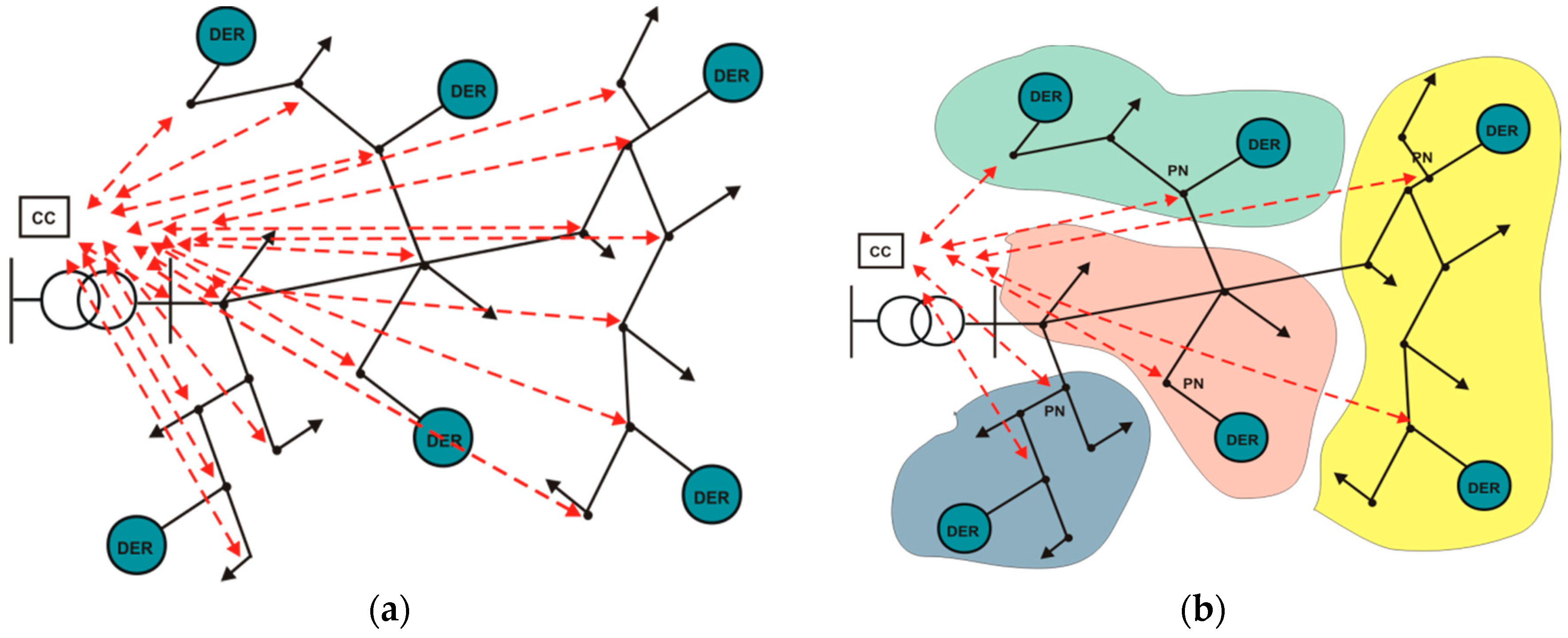
as highlighted in Figure 1a. Equation (23) is a non-linear programming problem of large dimension. Despite it provides the best solution of the voltage control problem, such an approach presents the following two drawbacks. Firstly, possible convergence problems may arise in the numerical solution, due to the non linear PF equations and to the large dimension; secondly, expensive communication infrastructure is needed to collect real-time measures from all DERs and loads.

To reduce the number of real-time measurements and to avoid using non linear PF equations, the linear modeling of the distribution system and its clustering into VCZs with PNs can be exploited as in [15]. Then, the minimization problem is rewritten in a variation form with respect to the initial operating point as:

$$\begin{gathered} \underset{\Delta P_k^{der}, \Delta Q_k^{der}}{\min }\sum _{h ϵ H_{pn}}{\left(\Delta V_h^2- \Delta V_{ref,h}^2\right)}^2 \\ \mathrm{subject}\mathrm{to}: \\ \Delta V_h^2=\sum _{k\in K_{der}}({\Gamma }_{P_{i,k}}\Delta P_k^{der}+{\Gamma }_{Q_{i,k}}\Delta Q_k^{der})h ϵ H_{pn} \\ \Delta V_{min,h}^2\le \Delta V_h^2\le \Delta V_{max,h}^2 h ϵ H_{pn} \\ \Delta P_{min,k}^{der}\le \Delta P_k^{der}\le \Delta P_{max,k}^{der} k ϵ K_{der} \\ \Delta Q_{min,k}^{der}\le \Delta Q_k^{der}\le \Delta Q_{max,k}^{der} k ϵ K_{der}, \end{gathered}$$

(24)

where:

• $\Delta V_h^2\triangleq V_h^2-{\left(V_h^2\right)}^0$ is the variation of the squared nodal voltage of the h-th PN with respect to the measured initial operating point ${\left(V_h^2\right)}^0$;
• $\Delta V_{ref,h}^2\triangleq V_{ref,h}^2-{\left(V_h^2\right)}^0$ is the variation of the squared reference value of the h-th PN with respect to ${\left(V_h^2\right)}^0$;
• $\Delta V_{min,h}^2\triangleq$$V_{min,h}^2-{\left(V_h^2\right)}^0$ and $V_{max,h}^2\triangleq$ $V_{max,h}^2-{\left(V_h^2\right)}^0$ are, respectively, the minimum and maximum variations of $\Delta V_h^2$;
• $\Delta P_k^{der}\triangleq P_k^{der}-{\left(P_k^{der}\right)}^0$ is the variation of the DER active power at the k-th node with respect to the initial operating point ${\left(P_k^{der}\right)}^0$;
• $\Delta Q_k^{der}\triangleq Q_k^{der}-{\left(Q_k^{der}\right)}^0$ is the variation of the DER reactive power at the k-th node with respect to the initial operating point ${\left(P_k^{der}\right)}^0$;
• $\Delta P_{min,k}^{der}\triangleq P_{min,k}^{der}-{\left(P_{h,k}^{der}\right)}^0$ and $\Delta P_{max,k}^{der}\triangleq P_{max,k}^{der}-{\left(P_{h,k}^{der}\right)}^0$ are, respectively, the minimum and maximum variations of $\Delta P_k^{der}$;
• $\Delta Q_{min,k}^{der}\triangleq Q_{min,k}^{der}-{\left(Q_{h,k}^{der}\right)}^0$ and $\Delta Q_{max,k}^{der}\triangleq Q_{max,k}^{der}-{\left(Q_{h,k}^{der}\right)}^0$ are, respectively, the minimum and maximum variations of $\Delta Q_k^{der}$.

In this way, the centralized voltage control can be achieved by:

• Measuring the voltage amplitude at the slack node;
• Collecting only the measures of the voltage amplitudes at the PNs;
• Solving a minimization problem subject to linear model (The linear model in (3) is reduced to the variations of the nodal voltage amplitudes) and network constraints;
• Sending the optimal set-points to the local controller of the DERs installed in the grid as highlighted in Figure 1b.

The main positive features of this formulation are: (i.) it does not present convergence problem due to the linearity of the model of the distribution system; (ii.) it requires a limited communication system because only the voltage amplitudes at the PNs are collected; (iii.) the convergence of the solving algorithm is guaranteed and the solution requires low computational burden, because it is a quadratic programming problem of small dimension. As a drawback, the solution of Equation (24) is an approximation of the solution of Equation (23) but very close to the optimal one, as shown in the case study, provided that the network has adequately been clustered.

5. Results

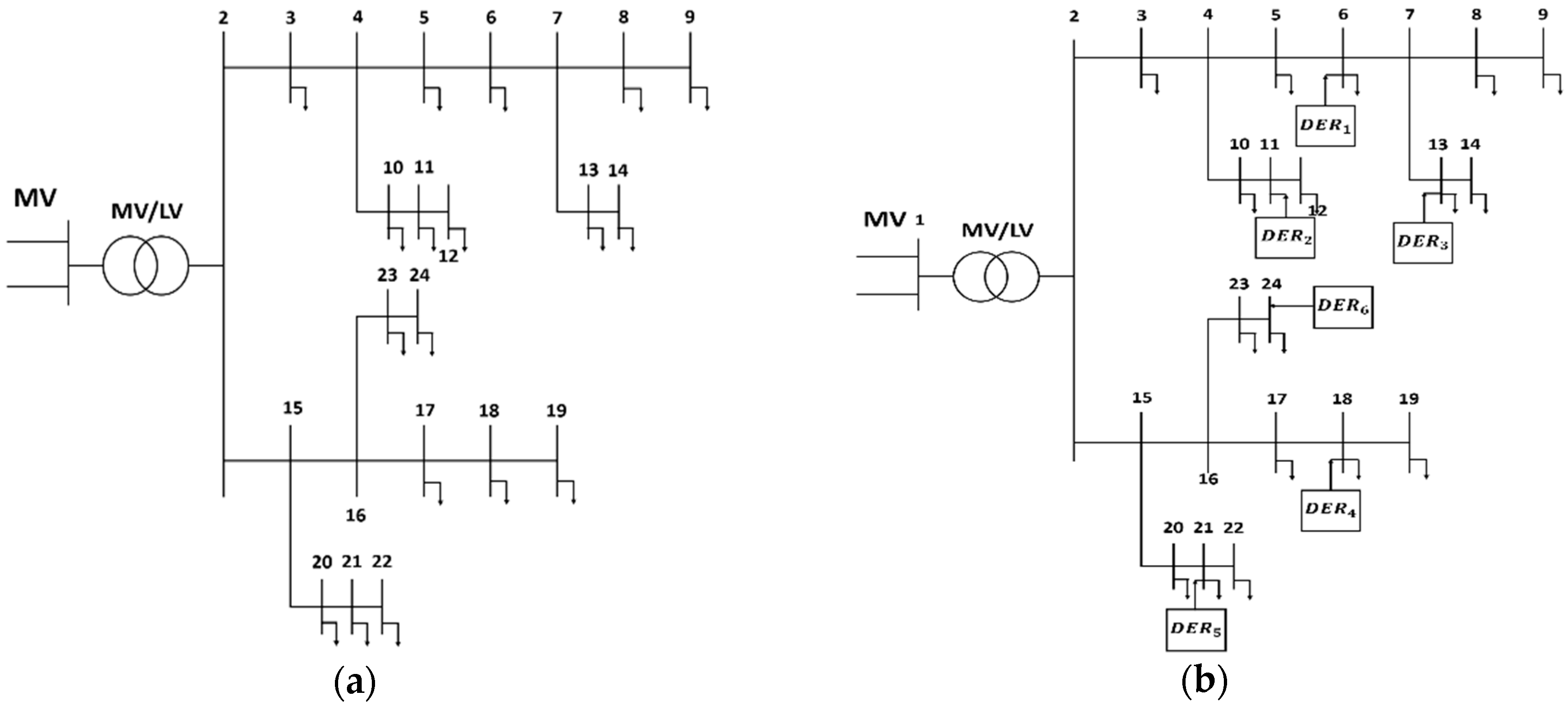
Reference is made to the 24-nodes LV distribution network in Figure 2a. A 20/0.4 kV substation with a 25 kVA transformer feeds a network with 22 nodes composed of 2 main feeders, each one with 2 laterals. Electrical parameters of lines and uncontrolled loads are reported in

Table 1. Electrical parameters of lines.

From Node	To Node	R (p.u.)	X (p.u.)	R/X
2	3	0.0105	0.0025	4.2
3	4	0.0059	0.0014	4.2
4	5	0.0114	0.0027	4.2
5	6	0.0079	0.0011	7.2
6	7	0.0095	0.0014	6.8
7	8	0.0053	0.0007	7.6
8	9	0.0040	0.0006	6.7
4	10	0.0106	0.0015	7.1
10	11	0.0121	0.0017	7.1
11	12	0.0040	0.0006	6.7
7	13	0.0089	0.0011	8.1
13	14	0.0037	0.0002	18
2	15	0.0006	0.0001	6.0
15	16	0.0190	0.0010	19
16	17	0.0100	0.0005	20
17	18	0.0088	0.0004	22
18	19	0.0408	0.0019	21
15	20	0.0038	0.0008	4.8
20	21	0.0512	0.0027	19
21	22	0.0236	0.0012	20
16	23	0.0632	0.0096	6.6
23	24	0.0017	0.0003	5.7

and

Table 2. Rated powers of uncontrolled loads.

From Node	Pload,r (kW)	Qload,r (kVAr)
2	3.11	1.56
3	3.11	1.56
4	2.04	1.01
5	2.04	1.01
6	7.93	3.97
7	2.04	1.01
8	3.11	1.56
4	3.11	1.56
10	3.11	1.56
11	3.11	1.56
12	3.11	1.56
13	3.11	1.56
14	3.11	1.56
15	9.84	4.91
16	7.93	3.97
17	3.11	1.56
18	3.11	1.56
19	7.93	3.97
20	7.93	3.97
21	2.04	1.01
22	7.93	3.97
23	2.04	1.01

, respectively. In the following the values in p.u. are referred to a power basis equal to 25 kVA.

Results are organized as follows. Zoning methodologies are firstly tested in the 24 nodes LV network with the aim to highlight their specific characteristics. Then, the applicability of the zoning techniques to the voltage optimization problem is investigated, with the aim to obtain a simplified representation of the LV network suitable for smart control of six DERs connected to the network, see Figure 2b.

5.1. Zoning Methodologies

The linear method is applied to evaluate the full $\left(3\times 2\right)$ sensitivity matrices ${\mathit{T}}_i\left(k\right)$ with $i,k=3, \dots , 24$ in the following assumptions:

• No-load voltage amplitude at the MV busbar: $V_{MV}=1.0$ p.u.;
• Active and reactive powers absorbed by uncontrolled loads equal to 70% of the rated values: $P_i^{load}$ = 70%$P_i^{load,r}$ and $Q_i^{load}$ = 70%$Q_i^{load,r}$;
• No DER connected to the grid.

Then, the sensitivity coefficients of the square nodal voltages to the DER active and reactive powers injections are extracted from the ($3\times 2)$ sensitivity matrices ${\mathit{T}}_i\left(k\right)$ with $i=3, \dots , 24$ (third row) and collected in the $\left(22\times 22\right)$ voltage sensitivity matrices, respectively, ${\mathit{\Gamma }}_P$ and ${\mathit{\Gamma }}_Q$, once and for all. The $(22\times 22$) matrices $\mathit{D}\left(0\right)$ of the electrical distances between any two nodes of the network are evaluated by the sensitivity measures reported in the following:

• Sensitivity to active power, referred to as ${\mathit{D}}_{\mathit{P}}\left(0\right)$;
• Sensitivity to reactive power, referred to as ${\mathit{D}}_{\mathit{Q}}\left(0\right)$;
• Sensitivity to active and reactive powers based on the Manhattan distance, referred to as ${\mathit{D}}_{\mathit{P}\mathit{Q}}^1\left(0\right)$;
• Sensitivity to active and reactive powers based on the Euclidean distance, referred as ${\mathit{D}}_{\mathit{P}\mathit{Q}}^2\left(0\right)$.

Nodes are merged in VCZs by applying the six different methodologies listed below (see Section 3):

• Hierarchical clustering with ${\mathit{D}}_P\left(0\right)$, referred to as P algorithm;
• Hierarchical clustering with ${\mathit{D}}_Q\left(0\right)$, referred to as Q algorithm;
• Hierarchical clustering with ${\mathit{D}}_P\left(0\right)$ and ${\mathit{D}}_Q\left(0\right)$, referred to as PQ algorithm;
• Intersection clustering with ${\mathit{D}}_P\left(0\right)$ and ${\mathit{D}}_Q\left(0\right)$, referred to as P ∩ Q algorithm;
• Hierarchical clustering with ${\mathit{D}}_{PQ}^1\left(0\right)$, referred to as D¹ algorithm;
• Hierarchical clustering with ${\mathit{D}}_{PQ}^2\left(0\right)$, referred to as D² algorithm.

and PNs are derived by using the algorithm reported in Section 3.3. Assigned the topology of the distribution network, for each zoning methodology, the three cases described in the following are considered to analyze the dependence of the results on the R/X ratio of the line parameters:

• Case R—In this base case, the R/X ratio of the line parameters are reported in Table 1. They are typical values of a LV network in which resistive parameters are prevailing; note that the different ratios are related to the presence of both lines and cables (R/X is higher for cables) and to difference sections (R/X is lower at the head of the feeder).
• Case R≈X—Each R/X ratio in Table 1 is multiplied for a factor equal to 0.2 so as to obtain comparable values of resistive and inductive parameters.
• Case X—Each R/X ratio in Table 1 is multiplied for a factor equal to 0.05; results are typical of a MV network in which inductive parameters are prevailing.

The results obtained by clustering the nodes of the distribution network into 3 VCZs are shown in

Table 3. Nodes and pilot nodes for three voltage control zones (VCZs).

Case	Algorithm	VCZ1		VCZ2		VCZ3
		Nodes	PN	Nodes	PN	Nodes	PN
R	P, PQ, D1, D2	3–14	5	15,20–22	20	16–19,23,24	17
	Q, P∩Q	3–14	5	15–22	16	23,24	23
R≈X	P, Q, PQ, P∩Q, D1, D2	3–14	5	15,20–22	20	16–19,23,24	18
X	P	3–15,20	5	16–19,23,24	16	21,22	21
	Q, PQ, D1, D2	3–14	5	16–19,23,24	16	15,20–22	20
	P ∩ Q	-	-	-		-	-

, reporting the nodes assigned to each VCZ and the corresponding PN (which are obtained by using the six different clustering algorithms) for the three considered cases of R/X ratios. In the Case R, most of the algorithms taking simultaneously into account the sensitivities of the nodal voltages to the active and reactive powers (i.e., PQ, D¹ and D²) gives rise to the same VCZs and PNs derived from the application of the P algorithm; this results was expected, since the network is predominantly resistive and, then, more sensitive to the active power injections. In the Case R≈X, VCZs and PNs are identical for all the clustering algorithms. In the Case X the result is opposite to the one in the Case R: since the network is predominantly inductive, all the algorithms that aggregate the sensibilities to the active and reactive powers (i.e., PQ, D¹ and D²) provide the same results of the Q algorithm; it is worth noticing that in this case the P∩Q algorithm does not provide an intersection of the network into three VCZs.

Similar results are reported in

Table 4. Nodes and pilot nodes for four VCZs.

Case	Algorithm	VCZ1		VCZ2		VCZ3		VCZ4
		Nodes	PN	Nodes	PN	Nodes	PN	Nodes	PN
R	P, D1, D2	3–14	5	15,20	20	16–19,23,24	17	21,22	21
	Q, P∩Q, PQ	3–14	5	15,20–22	20	16–19	17	23,24	23
R≈X	P, D1, D2	3–14	5	15,20	20	16–19,23,24	17	21,22	21
	Q, PQ	3–14	5	15,20–22	20	16–19	17	23,24	23
	P∩Q	-	-	-	-	-	-	-	-
X	P, P∩Q, D1, D2	3–14	5	15,20	20	16–19,23,24	17	21,22	21
	Q, PQ	3–14	5	15,20–22	20	16–19	17	23,24	23

,

Table 5. Nodes and pilot nodes for five VCZs.

Case	Algorithm	VCZ1		VCZ2		VCZ3		VCZ4		VCZ5
		Nodes	PN	Nodes	PN	Nodes	PN	Nodes	PN	Nodes	PN
R	P, P∩Q, PQ, D1, D2	3–14	5	15,20	15	16–19	18	21,22	21	23,24	23
	Q	3–4,10–12	10	5–9,13,14	7	16–19	18	15,20–22	20	23,24	23
R≈X	P, Q, P∩Q, PQ, D1, D2	3–14	5	15,20	15	16–19	18	21,22	21	23,24	23
X	P	3,4,10–12	10	5–9,13,14	7	15,20	15	16–19,23,24	16	21,22	21
	Q, P∩Q, PQ, D1, D2	3–14	5	15,20	15	16–19	17	21,22	21	23,24	23

,

Table 6. Nodes and pilot nodes for six VCZs.

Case	Algorithm	VCZ1		VCZ2		VCZ3		VCZ4		VCZ5		VCZ6
		Nodes	PN	Nodes	PN	Nodes	PN	Nodes	PN	Nodes	PN	Nodes	PN
R	P, Q, P∩Q, PQ, D1, D2	3,4, 10–12	10	5–9, 13,14	7	15,20	15	16–19	18	21,22	21	23,24	23
R≈X	P, Q, P∩Q, PQ, D1, D2	3,4, 10–12	10	5–9, 13,14	7	15,20	15	16–19	18	21,22	21	23,24	23
X	P, Q, P ∩ Q, PQ, D1, D2	3,4, 10–12	10	5–9, 13,14	7	15,20	15	16–19	18	21,22	21	23,24	23

and

Table 7. Nodes and pilot nodes for seven VCZs.

Case	Algorithm	VCZ1		VCZ2		VCZ3		VCZ4		VCZ5		VCZ6		VCZ7
		Nodes	PN	Nodes	PN	Nodes	PN	Nodes	PN	Nodes	PN	Nodes	PN	Nodes	PN
R	P	3,4, 10–12	10	5–9, 13,14	7	15	15	20	20	16–19	18	21,22	21	23,24	23
	Q	3,4,10	4	5–9, 13,14	7	11,12	11	15,20	15	16–19	18	21,22	21	23,24	23
	PQ, D1, D2	3,4	4	5–9, 13,14	7	10–12	11	15,20	15	16–19	18	21,22	21	23,24	23
	P∩Q	-	-	-	-	-	-	-	-	-	-	-	-	-	-
R≈X	P, Q, P∩Q, PQ, D1, D2	3,4	3	5–9, 13,14	7	10–12	11	15,20	15	16–19	18	21,22	21	23,24	23
X	P	3,4	3	5–9, 13,14	7	10–12	11	15,20	15	16–19	17	21,22	21	23,24	23
	Q, P∩Q, PQ, D1, D2	3,4, 10–12	10	5–9, 13,14	7	15,20	15	16–18	17	19	19	21,22	21	23,24	23
	P∩Q	-	-	-	-	-	-	-	-	-	-	-	-	-	-

for a network divided, respectively, in 4–7 VCZs. Referring to Table 4, both VCZs and PNs are the same for P, D¹ and D² algorithms as well as for Q and PQ algorithms, whatever the value of the R/X ratio; the P∩Q algorithm does not provide a solution in the Case R≈X. Although the clustered nodes of the VCZs are different, the resulting PNs are quite similar among the six algorithms and the three cases. The outcomes of the clustering of the network into five VCZs, reported in Table 5, exemplifies the most classical results. In the Case R, that is a network with dominant resistive parameters, all the algorithms follow the same clustering provided by the P algorithm, with the only exception of the Q algorithm; in the dual Case X, that is a network with dominant resistive parameters, the result is the opposite and all the algorithms follow the same clustering provided by the Q algorithm, with the only exception of the P algorithm; eventually, in the intermediate Case R≈X all six algorithms provide the same VCZs and PNs. Table 6 shows the VCZs and PNs in the case of a network clustered into six VCZs; surprisingly, results are the same for all the six algorithms and all the three cases. For the sake of completeness, Table 7 reports the results obtained by clustering the network into seven VCZs; indeed, they are of little significance because there are VCZs with only one node, due to the large number of VCZ with respect to the total number of network nodes.

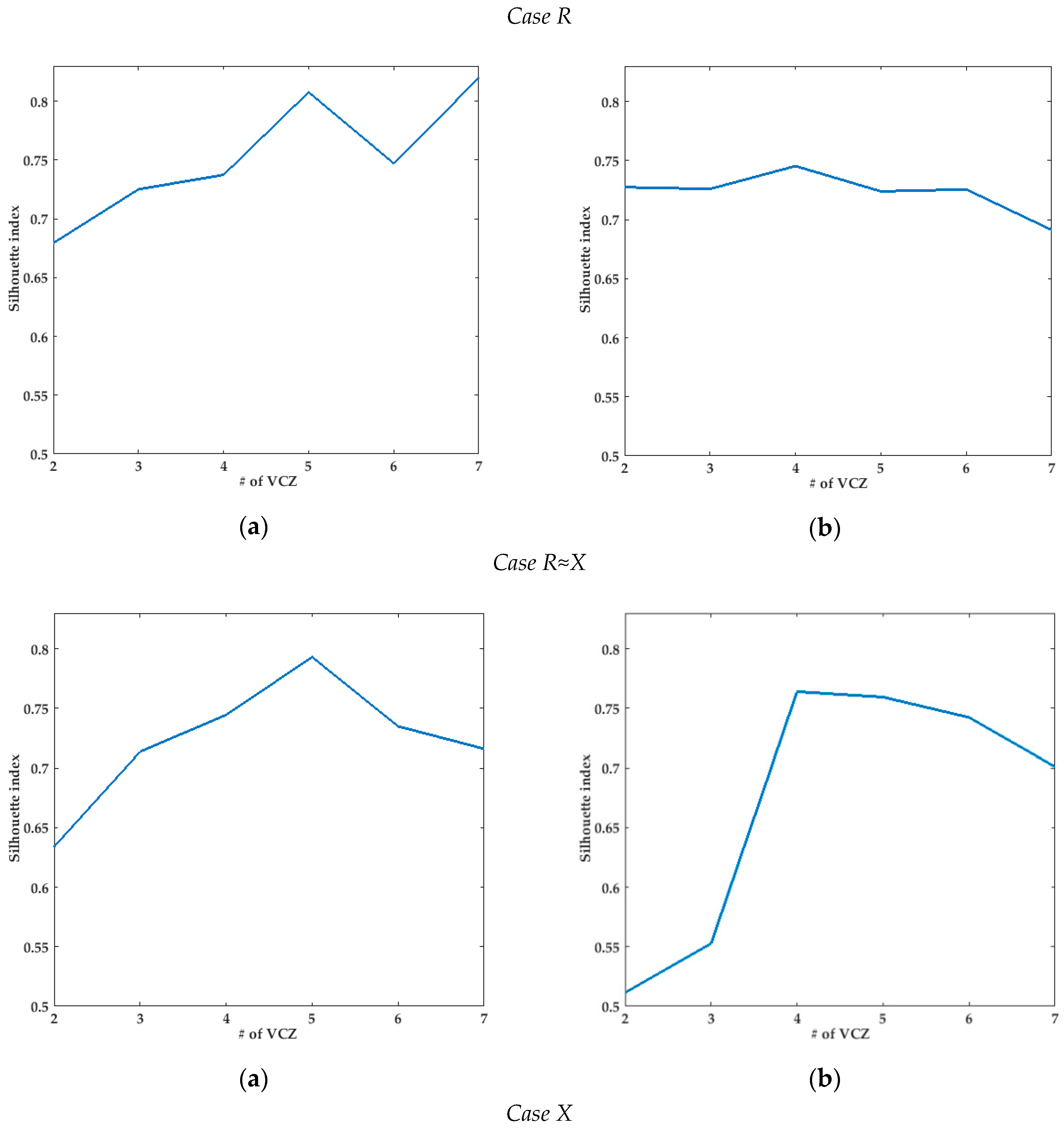
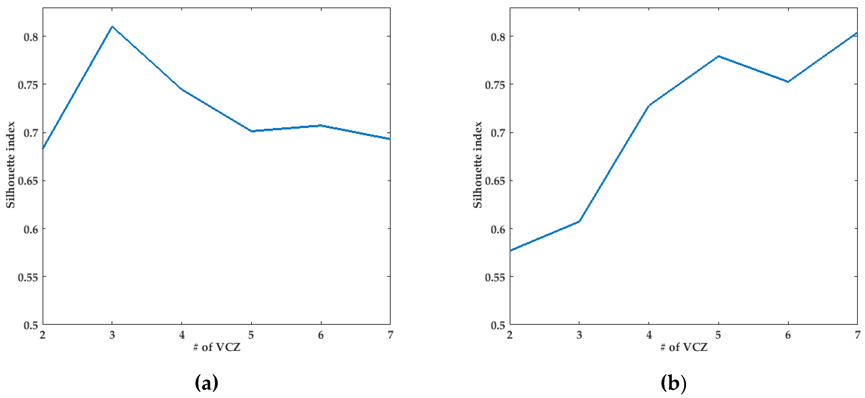
With reference to the P and the Q algorithms, the Silhouette index was calculated and plotted with respect to the number of VCZs in Figure 3, for the three considered cases. Comparing the first two plots in Figure 3 which refer to the Case R, the index is generally higher for the P algorithm as expected, because R is prevalent with respect to X; for the P algorithm the index increases in value with the increasing number of VCZ and the highest values are reached for VCZ $\ge 5$; for the Q algorithm the index has a slight peak for VCZ equal to 4. The second couple of plots refer to the Case R≈X; the index for the Q algorithm starts from a lower value for VCZ equal to 2 with respect to the previous Case R, then it increases rapidly to reach a peak for VCZ equal to 4 as previously; the index for the P algorithm is a bit smaller than the one for the Case R, but starting from a similar value for VCZ equal to 2, reaches its peak for VCZ equal to 5, then it decreases. In the last Case X, the index for the Q algorithm has a similar behavior as the one for the P algorithm in the first Case R, that was expectable; in fact, the index increases with the number of VCZ to get the best values for VCZ $\ge 5$. The index for the P algorithm has a peak for VCZ equal to 3, then it decreases with increasing number of VCZs. Some conclusions can be drawn:

• In the Case R, index for the P algorithm shows higher values and the best choice is for VCZ $\ge 5$;
• In the Case R≈X, both P and Q algorithms show the largest index value for VCZ = 5, considering that for the Q algorithm there is small variation of the index between VCZ equal to 4 or 5;
• In the Case X, the index for the Q algorithm suggests a clustering composed of VCZ equal to 5 or larger values whereas the index for the P algorithm has a peak for VCZ equal to 3.

5.2. Voltage Optimization Problem

To test the effectiveness of dividing the distribution network into VCZs, the PNs have been used to solve the voltage optimization problem in its reduced Equation (24). To this aim, 6 DERs are connected to the grid at nodes #6, #11, #13, #18, #21, #24, as shown in Figure 1b. Two DER configurations are considered to evaluate the impact of DER active and reactive powers injections/absorptions on the optimization of the voltage profiles:

• DG—DERs are DGs connected to the grid by inverters; they inject a fixed active power $P_i^{dg}$ = 20 kW and are equipped with a Volt/Var control with $Q_i^{dg}$=$\pm 15$ kVAr (the European Standards [31] impose that inverters of significant powers (greater than 11 kW) have a “rectangular capability chart”, which guarantees independence of the two powers in their admissible ranges. In the considered case, the inverter guarantees a “rectangular” capability chart that allows to vary the reactive power in the range [−15, 15] kVAr, independently from the value of the active power); in the initial operating point $Q_i^{dg}$=$0$ kVAr.
• DG and BESS—DERs are DGs connected to the grid by inverters that inject a fixed active power $P_i^{dg}$ = 10 kW and that are equipped with a Volt/Var control with $Q_i^{dg}$ = $\pm 15$ kVAr (in the initial operating point $Q_i^{dg}=0$ kVAr); DGs connected to nodes #6, #11, #18, #24 are also equipped with BESSs injecting/absorbing a controlled active power $P_i^{bess}$; it is assumed that the state-of-charge of the BESSs allows to vary $P_i^{bess}$ in the range [−5, 5] kW.

To measure the performance of the Proposed VOP, the optimal solution must firstly be obtained. To this aim, for each Case and each DER configuration, firstly the minimization problem (23), optimizing all the nodal voltages with the PF equations as constraints, is solved by optimal power flow algorithm in MATPOWER [32]. In these problems, as well as in all the problems in the remainder, it is assumed $V_{ref,i}$= 1.0 p.u. for all i. The optimal solution is expressed in terms of set-points of the powers injected by DERs and the resulting voltage profile is the optimal one for the considered case, thus it is referred to as Benchmark. Then, the proposed problem (24), optimizing the voltages of the only PNs with the constraints derived from the linear model of the distribution system, is solved by classical quadratic programming algorithm in MATLAB^®; in the following this problem is referred to as proposed voltage optimization problem (VOP).

Numerous VOPs have been formulated and solved considering different numbers of VCZs (from three to six) and different clustering algorithms, in particular the P and the Q algorithms as described in the previous Section 3.1. The solutions of the proposed VOP are the variations of the set-points of the powers injected by DERs with respect to the initial operating point. Once the set-points are derived, such power injections are used to solve a power flow in MATPOWER so as to obtain the resulting voltage profile, which is also used to evaluate the value of the objective function of problem (23) in such suboptimal solution. Some results are presented in the following to evidence the main results that have been obtained.

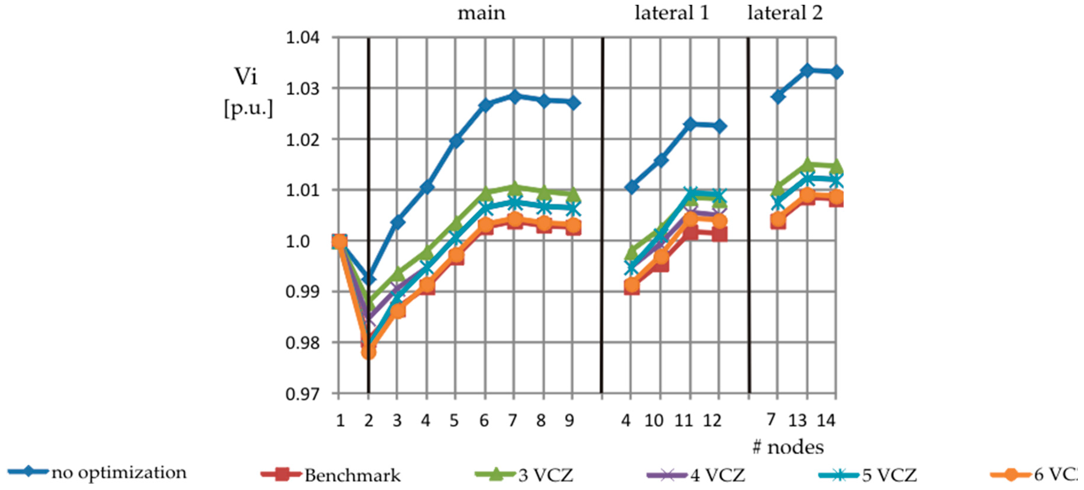
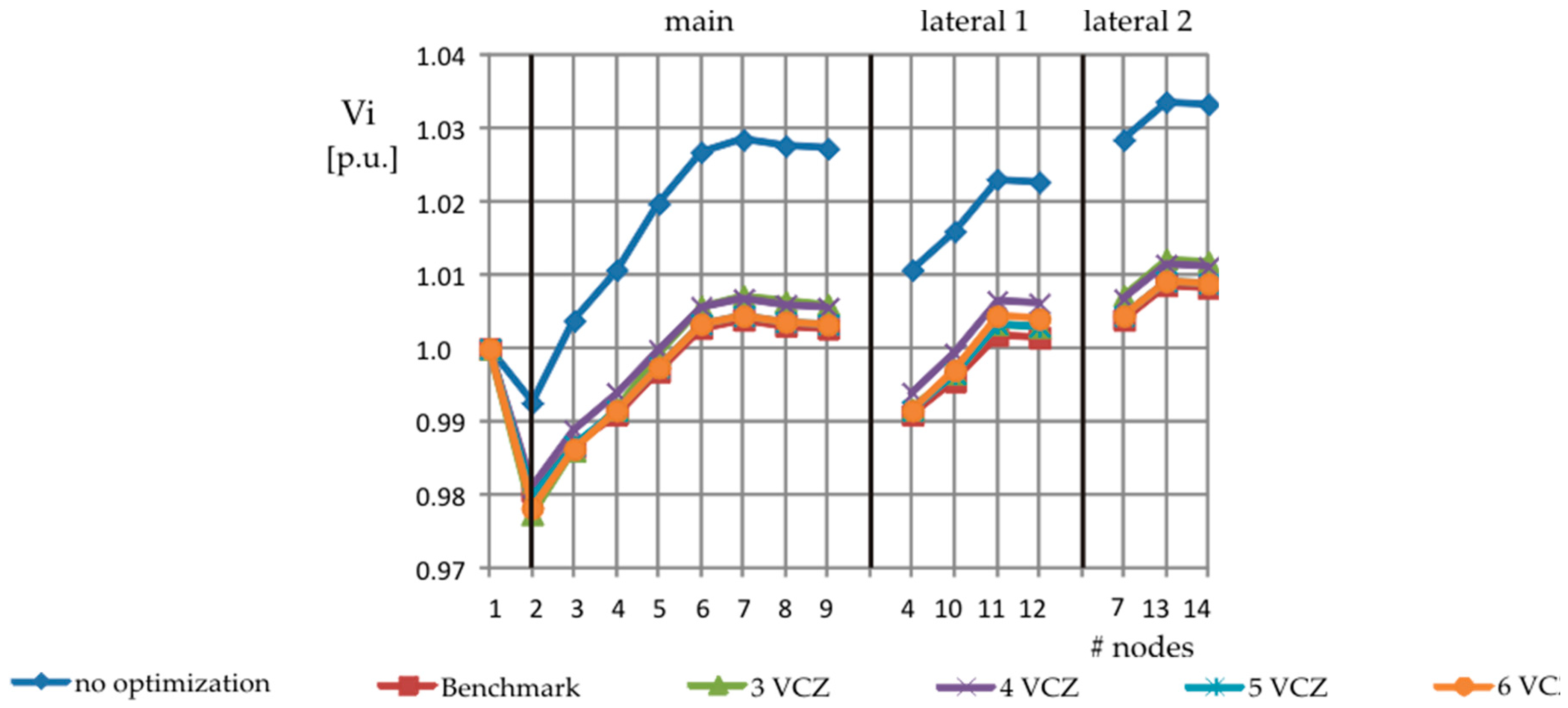
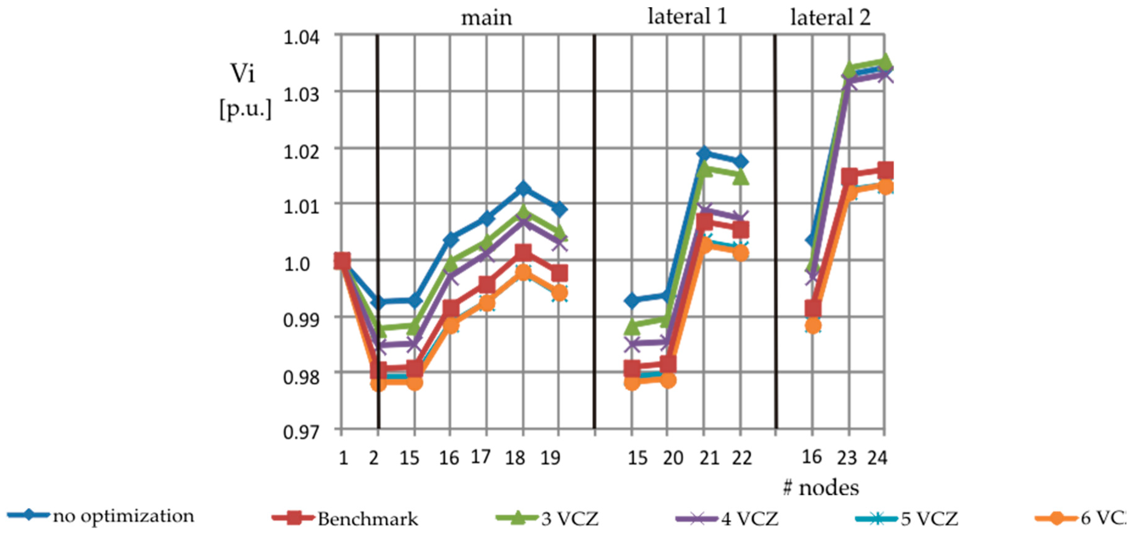
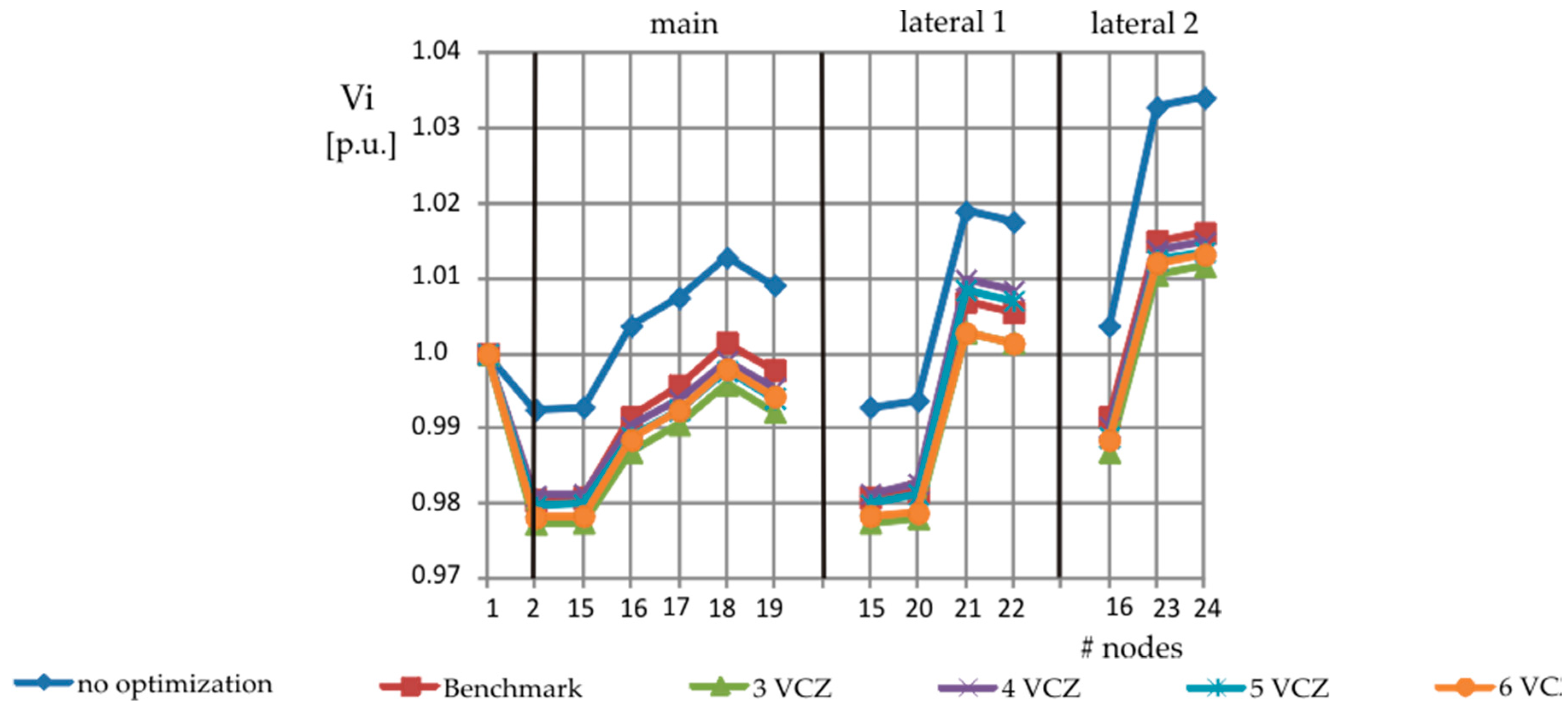
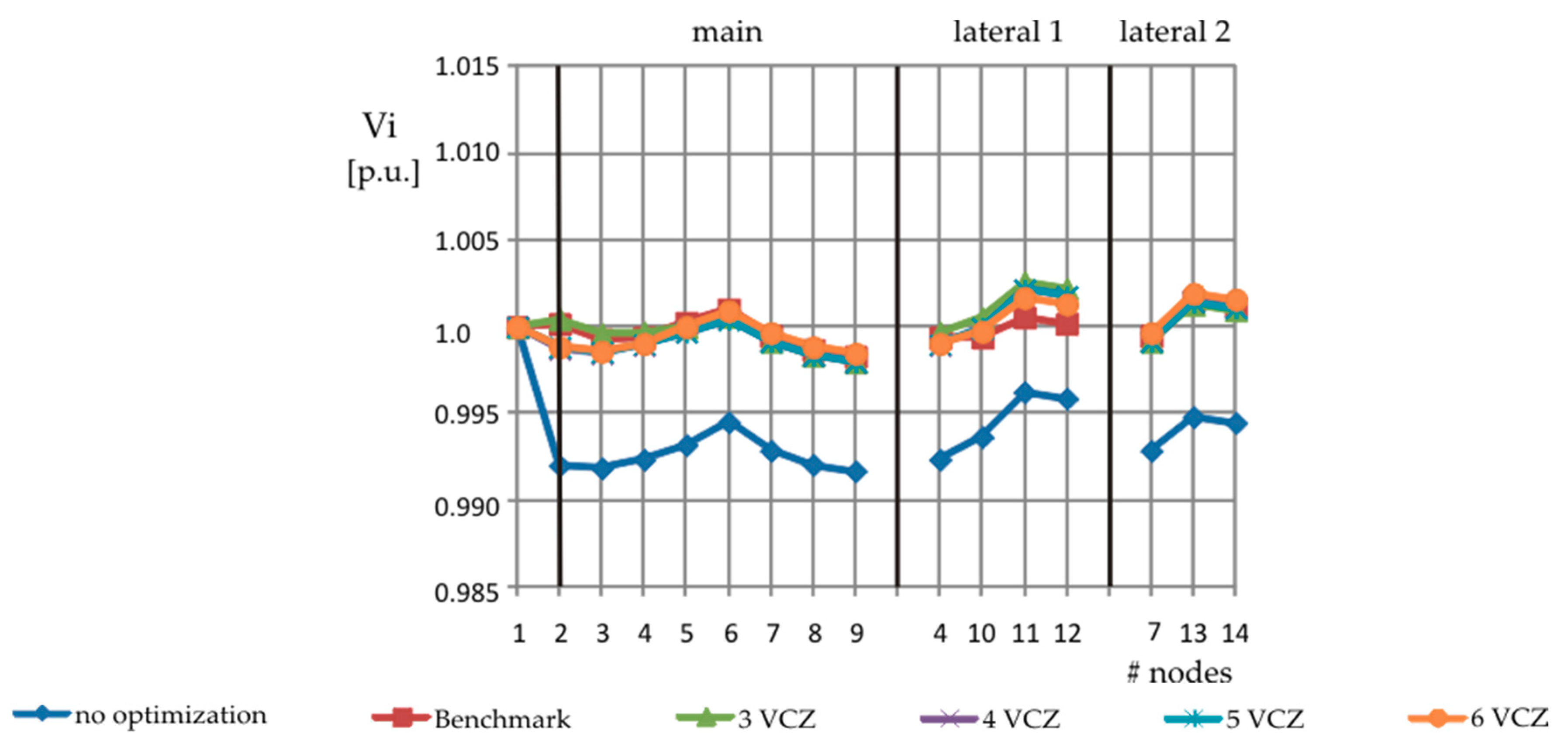
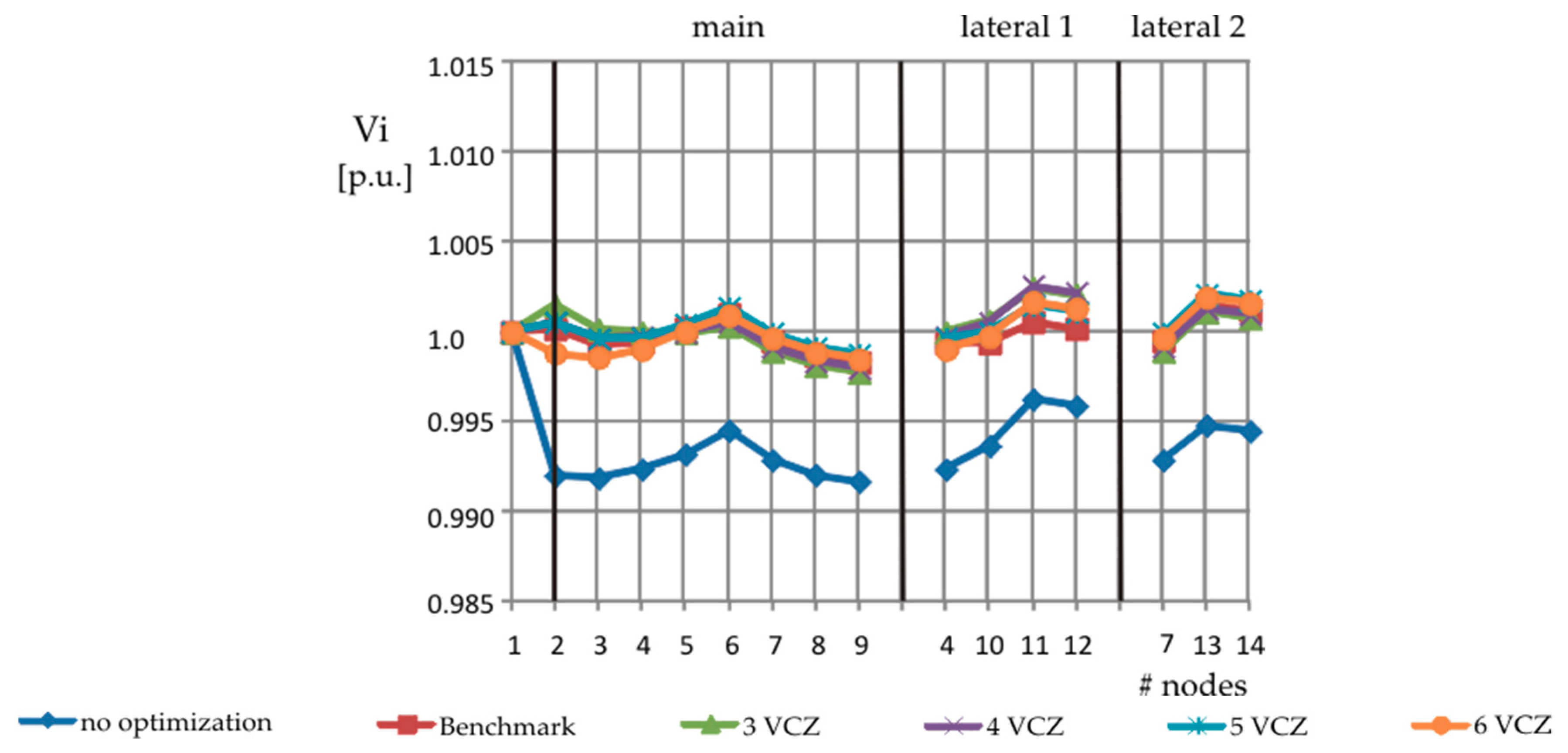
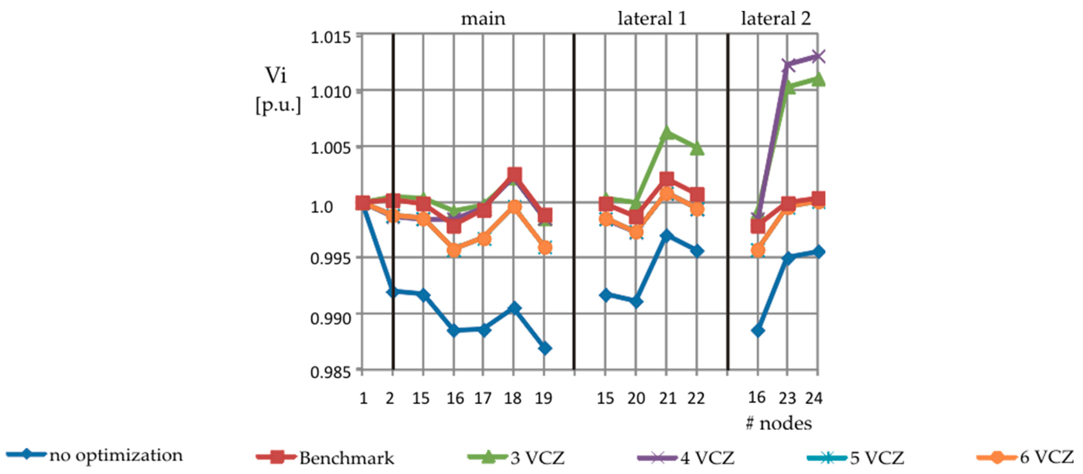
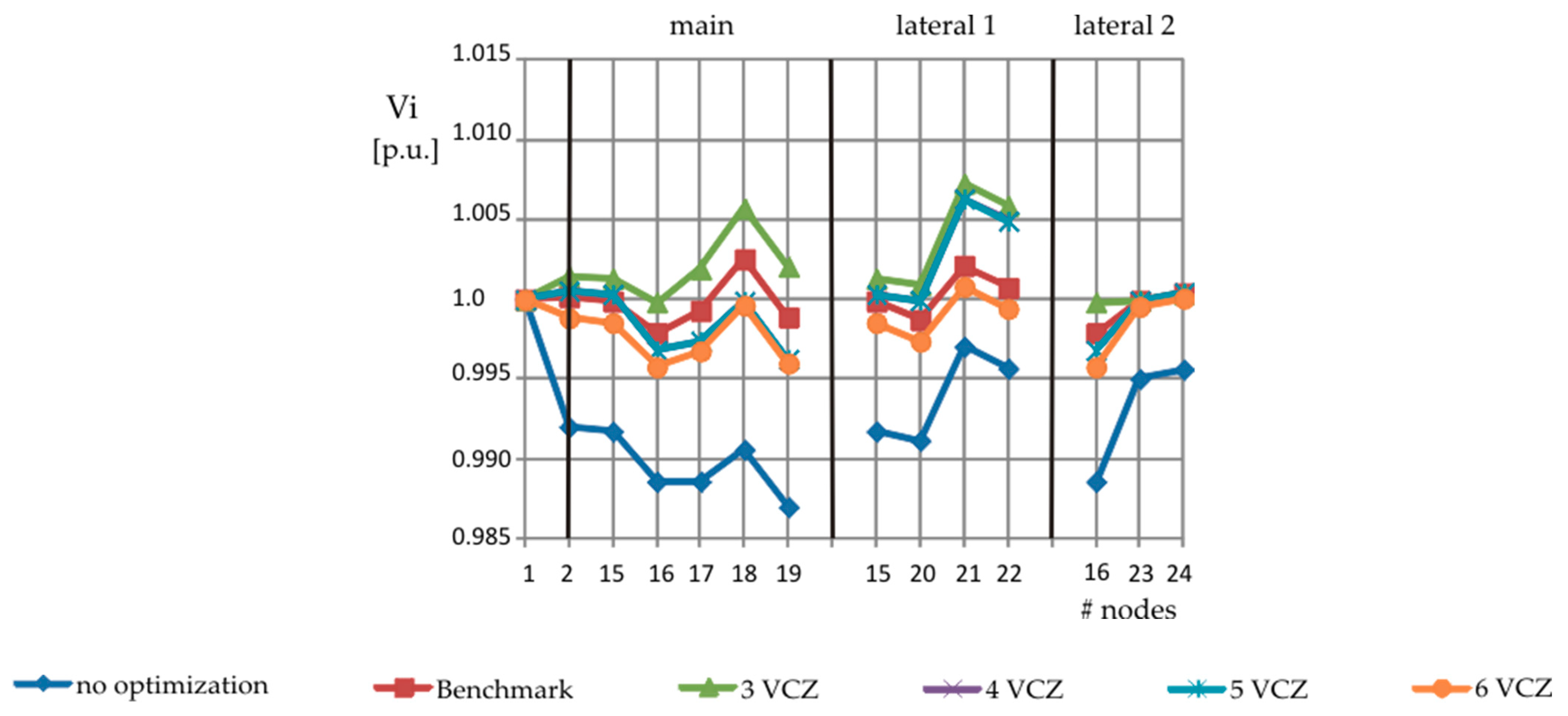
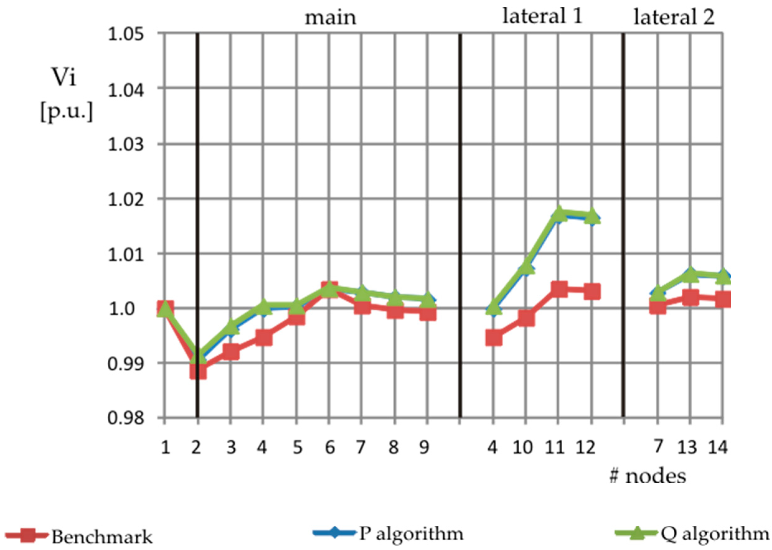
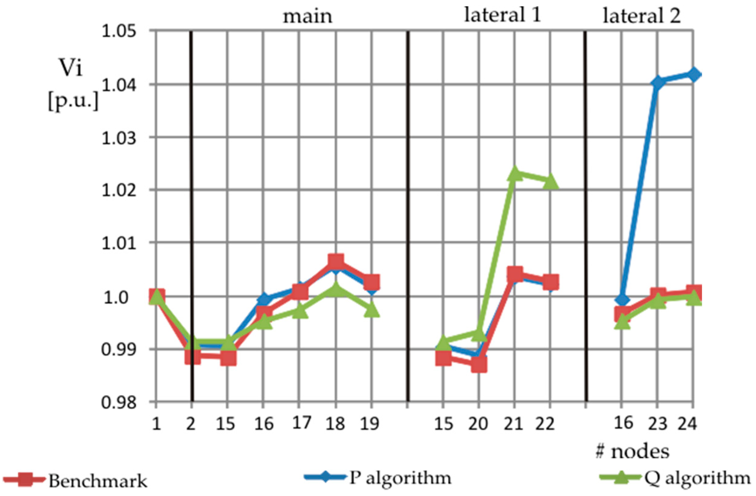
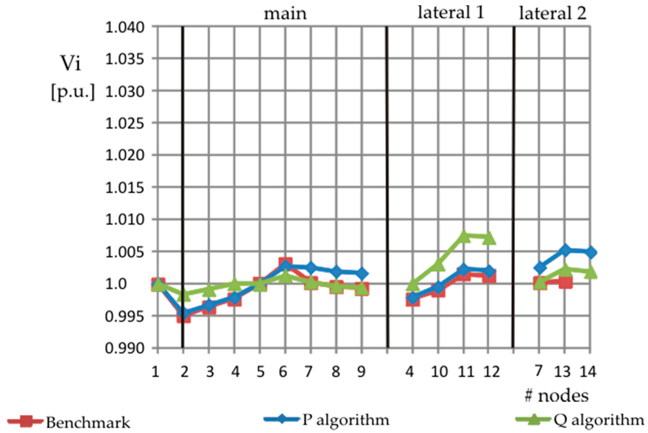
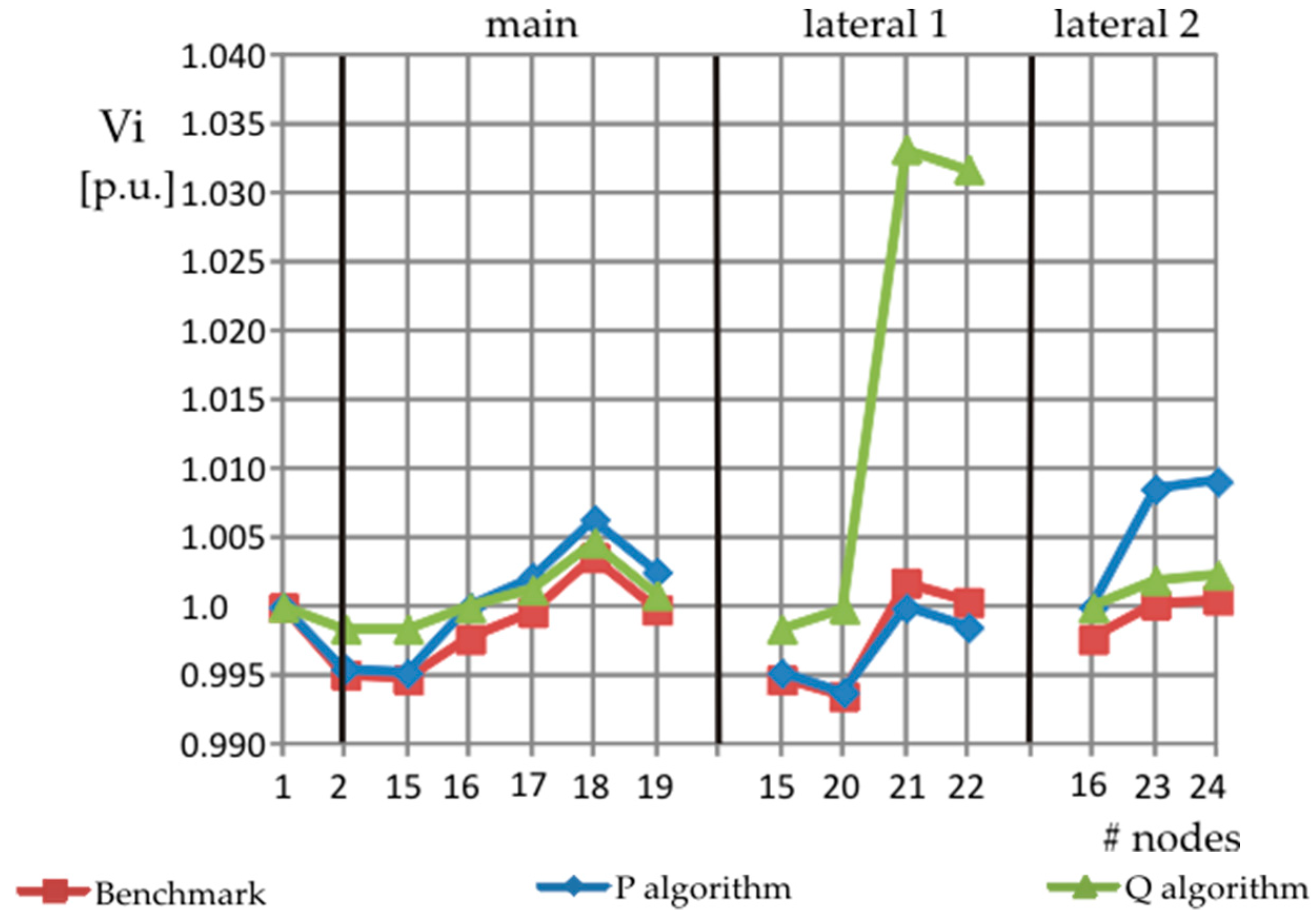
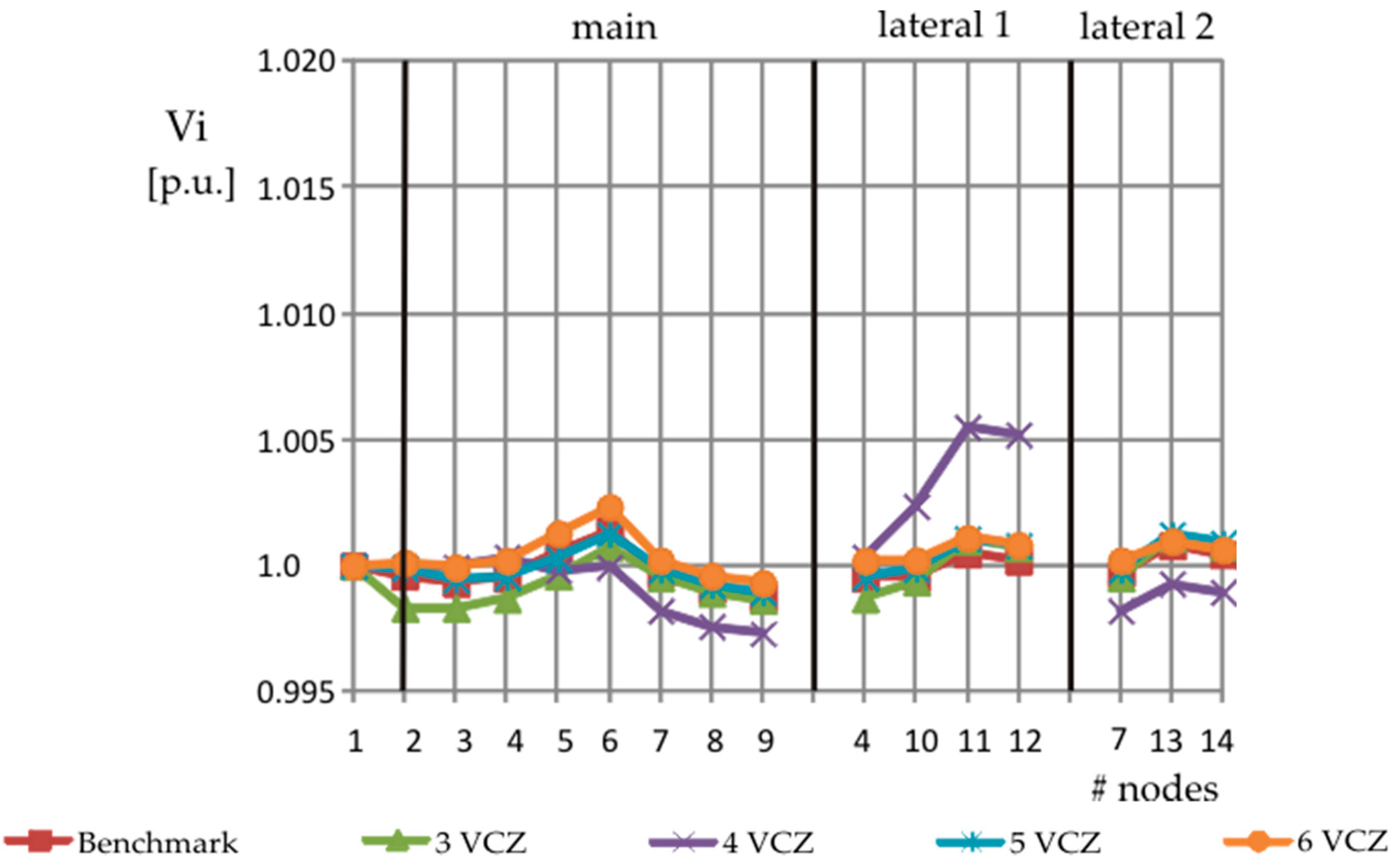
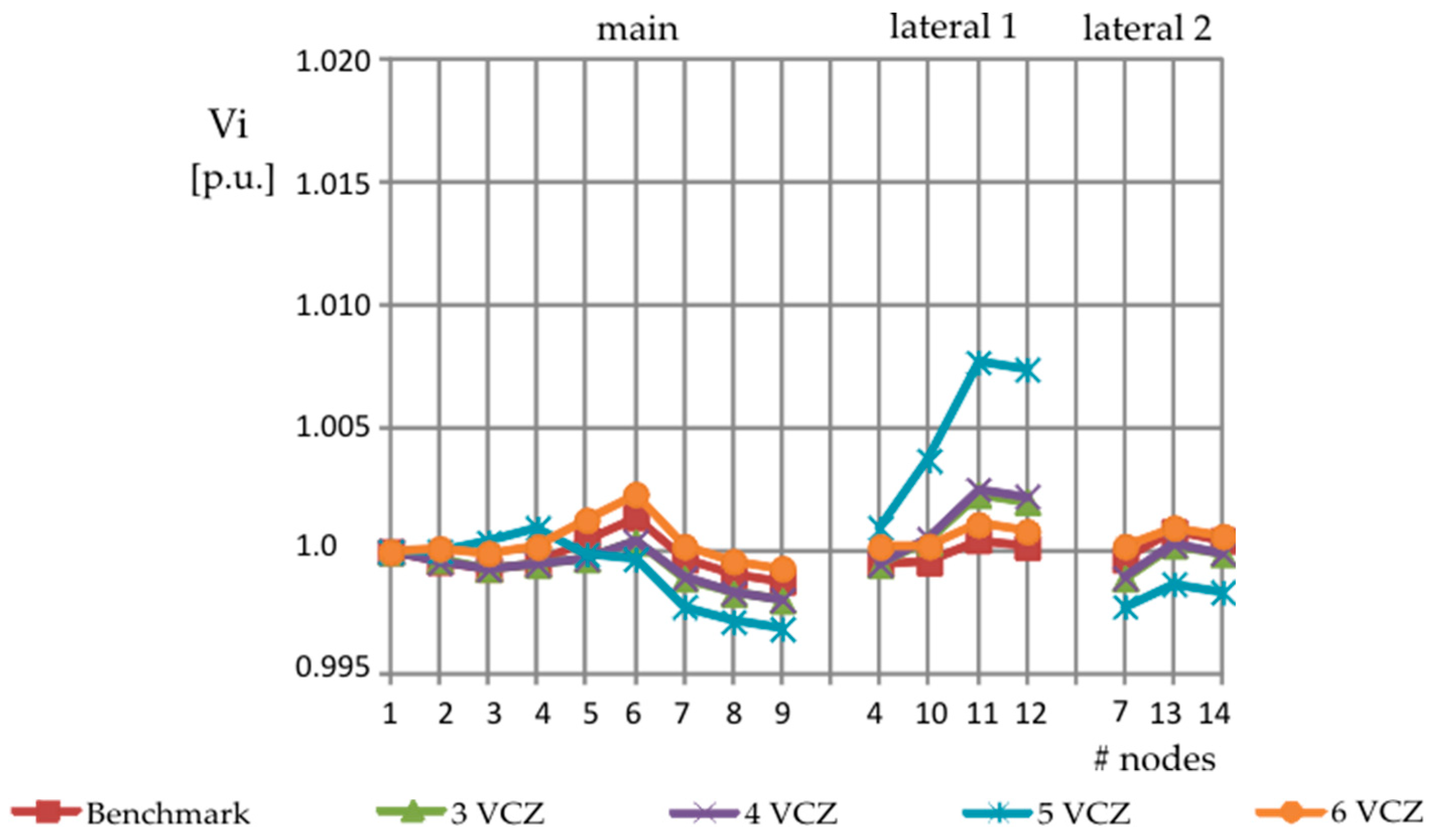
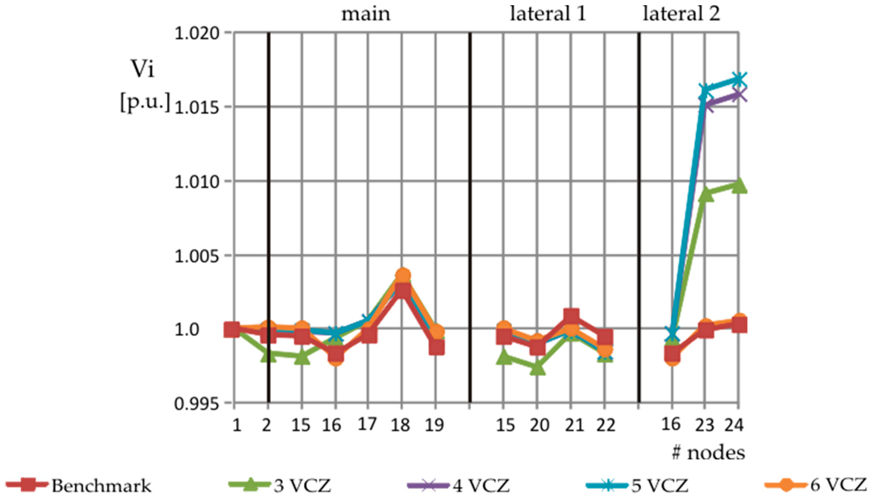
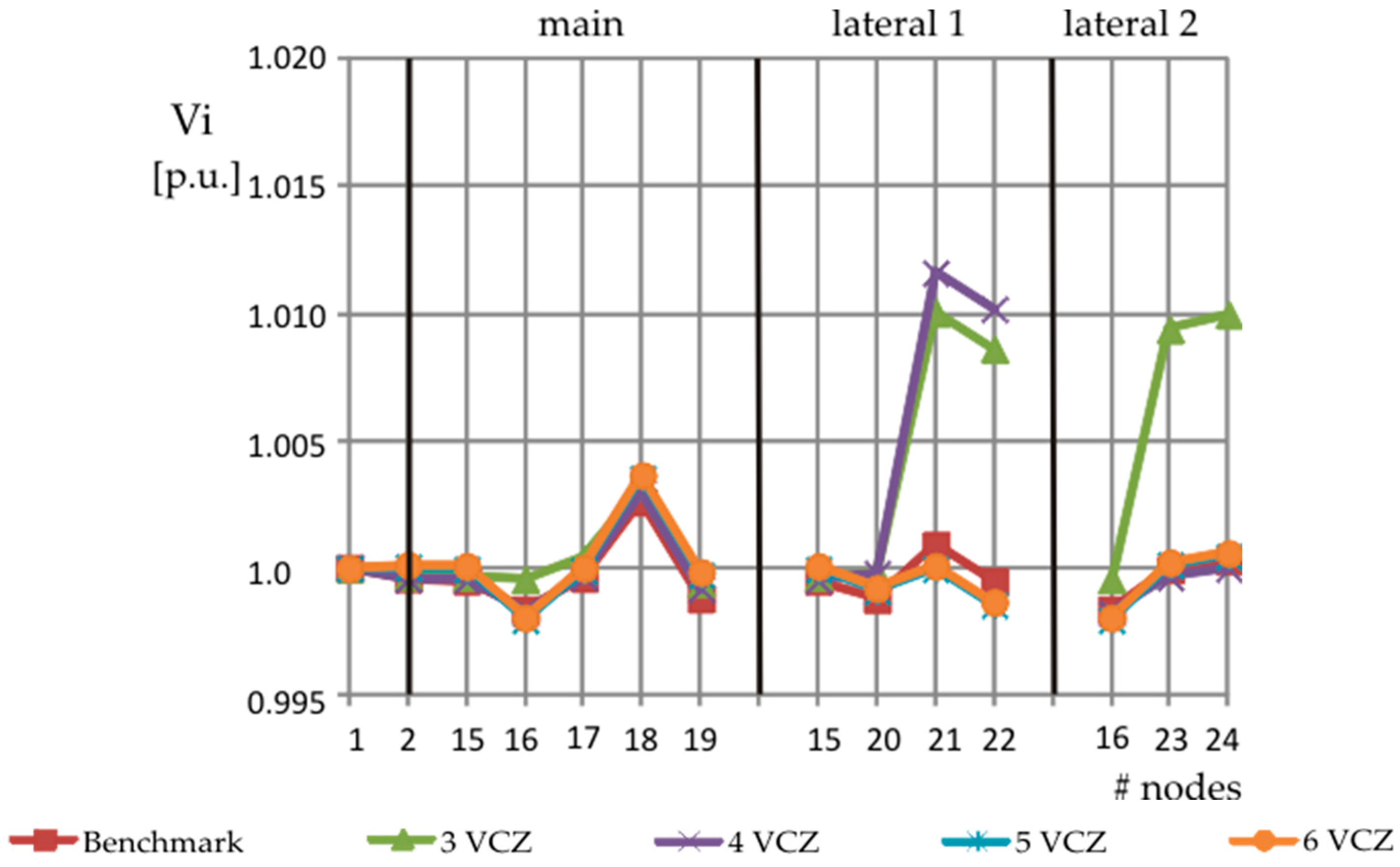
Always referring to the Case R—DG, the nodal voltage profiles are shown, along feeder 1 for P and Q algorithms, respectively, in Figure 4 and Figure 5, along feeder 2 for P and Q algorithms, respectively, in Figure 6 and Figure 7. Different profiles are plotted in each graph: the blue line refers to the voltage profile with DGs and $Q_{ref,i}^{dg}=0$ for all i; the red line refers to the Benchmark; the other lines refer to the voltage profiles obtained by the proposed VOP applied to different numbers of VCZs (from 3 to 6). The blue profile is not strictly decreasing along both the feeders because of the presence of DGs. In particular, DGs connected to the feeder 1 determine an increase of the voltage amplitudes in the main from nodes #3 to #7 as well as in the lateral 1 at nodes #10 and #11 and in the lateral 2 at node #13. Similarly, DGs connected to the feeder 2 determine an increase of the voltage amplitudes from nodes #15 to #18 in the main, at nodes #20 and #21 in the lateral 1 and at nodes #23 and #24 in the lateral 2. Despite the voltage rise, the voltage amplitudes are within the acceptable range for all the nodes.

Referring to the first DER configuration (DG) when the resistive parameters of the LV network are prevailing (Case R—DG),

Table 8. Normalized objective functions (p.u.) for Case R—DG.

Case	Configuration	Algorithm	Benchmark	Proposed VOP
				3 VCZ	4 VCZ	5 VCZ	6 VCZ
R	DG	P	1.0	2.4	1.9	1.2	1.1
		Q		1.3	1.1	1.1

reports the values of the objective function obtained by the proposed VOP and normalized with respect the Benchmark, which in this case is equal to 7.3 10⁻³ p.u. As evident from Table 8, the obtained values are of the same order of magnitude as the Benchmark: thus, the results can be considered substantially equivalent, with a slightly-better performance of the Q algorithm. It is interesting to underline that, in spite of the similarity of the values of the objective function, the proposed VOP provides solutions which significantly differ from the Benchmark in terms of the set points for the DG reactive powers $Q_{ref,i}^{dg}$ at nodes #11, #18, #21, as shown in

Table 9. Set-point $Q_{ref,i}^{dg}$ (kVAr) for Case R—DG.

		Reactive Power
Nodes	Algorithm	Benchmark	Proposed VOP
			3 VCZ	4 VCZ	5 VCZ	6 VCZ
#6	P	−15	−15	−15	−15	−15
	Q		−8.6
#11	P	−14	−15	−15	15	0.60
	Q		−8.8	−1.4	–7.2
#13	P	−15	−15	−15	−15	−15
	Q		−8.9
#18	P	15	−3.6	13	−9.6	−9.9
	Q		−11	−15	−15
#21	P	−4.3	15	−15	−15	−14
	Q		−9.3	15	15
#24	P	−15	15	15	−15.0	−15
	Q		−15	−15

.

All the optimizations result into an improvement of the voltage profiles, because the nodal voltage amplitudes are closer to $V_{ref,i}$=1.0 p.u. The Benchmark provides the best solution by decreasing the set-points $Q_{ref,6}^{dg}$, $Q_{ref,11}^{dg}$, $Q_{ref,13}^{dg}$, $Q_{ref,21}^{dg}$ and $Q_{ref,24}^{dg}$ thus reducing the nodal voltages through an inductive reactive power absorption, and by increasing $Q_{ref,18}^{dg}$. The values of the nodal voltage amplitudes obtained by the proposed VOP are quite similar to the Benchmark. Considerations about the improvement of the objective functions when the number of the VCZs increases as well as about the preference of the Q algorithm are confirmed observing the voltage profiles from Figure 4 to Figure 7.

Concerning to the Case R—DG and BESS,

Table 10. Normalized objective functions (p.u.) for Case R—DG and BESS.

Case	Configuration	Algorithm	Benchmark	Proposed VOP
				3 VCZ	4 VCZ	5 VCZ	6 VCZ
R	DG with BESS	P	1.0	11	12	2.5	2.4
		Q		5.0	3.8	3.6

reports the obtained values of the objective function normalized to the Benchmark, which in this case is equal to 0.12·10⁻³ p.u. and, then, significantly lower than the one in the previous Case R—DG. This is due to the possibility of varying also the active powers of BESSs which has a significant impact in a predominately-resistive network. From Table 10 it is evident that the results are substantially equivalent to the Benchmark with the only exceptions of the clustering into three and four VCZs provided by the P alghoritm which are significantly worse; for five VCZs the P algorithm shows a better result than the Q algorithm.

Table 11. Set-points $P_{ref,i}^{bess}$ (kW) and $Q_{ref,i}^{dg}$ (kVAr) for Case R—DG and BESS.

		Active Power					Reactive Power
Nodes	Algorithm	Benchmark	Proposed VOP				Benchmark	Proposed VOP
			3 VCZ	4 VCZ	5 VCZ	6 VCZ		3 VCZ	4 VCZ	5 VCZ	6 VCZ
#6	P	−4.1	−3.5	−3.8	−4.0	−3.4	15	5.2	8.1	8.3	8.5
	Q		−4.6	−3.6	−2.6			6.1	5.3	5.5
#11	P	−5.0	−1.8	−1.9	−2.0	−2.5	15	5.6	8.5	8.8	8.7
	Q		−2.4		−3.0			6.6	5.7	5.5
#13	P	-	-				3.3	5.1	8.1	8.2	8.3
	Q							6.1	5.3	5.5
#18	P	3	1.0	2.0	2.0	2.0	15	6.3	9.4	9.7	9.7
	Q		5.0	1.0	1.0			9.4	6.5	6.5
#21	P	-	-				-15	7.3	−15	−15	−15
	Q							7.5	7.5	7.4
#24	P	−2	1.0	2.0	−2.2	−2.3	1.9	6.3	9.5	9.1	9.1
	Q		−3.1	−2.2	−2.1			4.5	6.0	5.9

reports the resulting set-points for the active power aborbed/injected by BESS $P_{ref,i}^{bess}$ and for the reactive power absorbed/injected by DG $Q_{ref,i}^{dg}$. The active powers injected at nodes #13 and #21 are always equal to zero since no BESSs are installed. The optimal solution of the Benchmark is different from the ones given by the proposed VOP; indeed, the set points $P_{ref,i}^{bess}$ are rather similar whereas the set points $Q_{ref,i}^{dg}$ of the proposed VOP hardly ever reach the saturation values differently from the Benchmark, as highlighted in bold in Table 11. Always referring to the Case R—DG and BESS, the nodal voltage profiles are shown, along feeder 1 for P and Q algorithms, respectively, in Figure 8 and Figure 9, along feeder 2 for P and Q algorithms, respectively, in Figure 10 and Figure 11. In absence of optimization (blue line) the voltage profile is within the acceptable range, although characterized by a voltage rise at the nodes with DGs. All the optimizations flatten the voltage profiles around the reference values equal to 1.0 p.u.

The optimal voltage profile (red line) is obtained by injecting reactive powers by DGs and by absorbing active powers by BESSs. In fact, the reactive power mainly affects the voltage drop of the MV/LV transformer; then, the reactive power injections allow to increase the voltage at the LV busbar of the substation around 1.0 p.u. As counter effect, the voltages would rise above 1.0 p.u. along the feeders where DGs are connected; then, the active power absorptions by BESSs flatten the nodal voltages around the reference values, since in a resistive network the impact of the BESS on the voltage drops along the feeders is dominant. The values of the nodal voltage amplitudes obtained by the proposed VOP are quite similar to the optimal ones, except for the cases of three VCZs and four VCZs clustered according to the P algorithm, in which the voltage profile of the feeder 2 is far from the reference values, thus explaining the results in Table 10. Similarly to the previous case, the voltage profiles improve when the number of the VCZs increases.

Table 12. Normalized objective functions (p.u.) for Case R≈X.

Case	Configuration	Benchmark	Proposed VOP
			Algorithm	3 VCZ	4 VCZ	5 VCZ	6 VCZ
R≈X	DG	1.0	P	7.1	8.7	2.8	1.2
			Q		3.8
	DG and BESS	1.0	P	15	25	3.3	2.3
			Q		7.0

shows the objective functions of the Benchmark and the proposed VOP for, the Case R≈X with reference to the two DER configurations. The values are normalized with respect to the corresponding Benchmarks, which are equal to 2.1·10⁻³ p.u. and 0.12·10⁻³ p.u., respectively, for the configuration DG and the configuration DG and BESS. In a distribution network with comparable resistive and inductive line parameters, the evaluation of VCZs resulting from the application of the P and Q algorithms are equivalent in terms of the resulting values for the objective function. In fact, for both the DER configurations, the two zoning algorithms yield the same solution, except for the case of four VCZs. However, the errors of the proposed VOP become acceptable starting from five VCZs. As an example, Figure 12 and Figure 13 show the nodal voltage profiles of, respectively, feeder 1 and feeder 2 for the benchmark and the proposed VOP with four VCZs in the Case R≈X—DG. From Figure 12 the overlapping of the voltage profiles along feeder 1 obtained by the proposed VOP for the P and the Q algorithms is evident. Conversely, along the feeder 2 the benchmark is well followed by the P algorithm as far as the main and the lateral 1 are considered, whereas the Q algorithm presents a better performance for the lateral 2. The poor performance of the proposed VOP with the P algorithm is related to the absence of a PN belonging to lateral 2 (see Table 5) and is confirmed by the high value of the objective function (see Table 12).

Table 13. Normalized objective functions (p.u.) for Case X.

Case	Configuration	Benchmark	Proposed VOP
			Algorithm	3 VCZ	4 VCZ	5 VCZ	6 VCZ
X	DG	1.0	P	3.0	28	24	1.2
			Q	19	20	7.5
	DG with BESS	1.0	P	11	28	28	1.5
			Q	19	13	8.6

shows the normalized objective functions of the Benchmark and the proposed VOP for the Case X with reference to the two DER configurations. In general, the results obtained using the Q algorithm are better than the ones of the P algorithm, as expectable in a predominantly-inductive distribution network. The values of the objective function for the P algorithm are of one order of magnitude greater than the Benchmark, except for the case of three VCZs and for the case of six VCZs.

Figure 14 and Figure 15 show the nodal voltage profiles of, respectively, feeder 1 and feeder 2 for the Benchmark and the Proposed VOP with three VCZs in the Case X—DG. The P algorithm provides the best approximation of the optimal solution when three VCZs are adopted and this result is coherent with the better performance of Silhouette index for the P algorithm for 3 VCZs in the Case X, see Figure 3. This is due to the choice of node #20 as PN by the Q algorithm that gives rise to a high difference of the voltage amplitudes at node #21 of the Benchmark and the proposed VOP (Figure 14). From Table 13, it would seem that results have become acceptable starting from six VCZs. Actually, taking into account that the objective functions of the Benchmark are equal to 0.50 10⁻³ p.u. and 0.08 10⁻³ p.u. for, respectively, the DGs and the DGs with BESS configurations, the voltage regulation provides good performance also for a reduced number of VCZs. As an example, for the Case X—DG and BESS the nodal voltage profiles are shown, along feeder 1 for P and Q algorithms, respectively, in Figure 16 and Figure 17, along feeder 2 for P and Q algorithms, respectively, in Figure 18 and Figure 19.

6. Conclusions

The problem of the voltage profile optimization in a distribution system including distributed energy resources has been tackled adopting a centralized approach. To avoid the monitoring of a large number of electrical quantities in the distribution network as well as the solution of a large nonlinear programming problem, the voltage optimization has been re-formulated as a quadratic programming of reduced dimension based on control zones. The voltage control zones have been identified on the basis of the structural characteristics of the power grid (independently from the number and position of the distributed energy resources) and account for the sensitivity of the nodal voltages on active and reactive powers. General considerations can be made, although derived from a case study. First of all, the proposed voltage optimization problem always guarantees an improvement of the voltage profile; it gives a suboptimal solution which is quite similar to the optimal one provided that an adequate number of voltage control zones is used. Concerning the choice of the algorithm for the aggregation of the voltage control zones, the use of the voltage sensitivities on the reactive power is preferable if the voltage control acts on the reactive power injections/absorptions, as easily foreseeable. When the control acts on both active and reactive powers, the choice is to be related to the R/X ratio of the distribution lines. In fact, in predominantly-inductive networks, such as MV networks, better performance is achieved if the aggregation is based on sensitivities to reactive powers. On the other hand, in the case of LV distribution networks with predominantly-resistive lines, the distributed energy resources impact on the substation busbar voltage mainly through the reactive powers and on the shape of the voltage profile along the feeders mainly through the active powers; consequently, it is advisable to use an aggregation algorithm based on the sensitivities to both active and reactive powers. Finally, the proposed formulation of the voltage optimization problem based on voltage control zones is by its nature oriented to the decentralized control, whose implementation is the future step of this research.

References

- Efkarpidis, N.; De Rybel, T.; Driesen, J. Technical assessment of centralized and localized voltage control strategies in low voltage networks. Sustain. Energy Grids Netw. 2016, 8, 85–97. [Google Scholar] [CrossRef]
- Antoniadou-Plytaria, K.E.; Kouveliotis-Lysikatos, I.N.; Georgilakis, P.S.; Hatziargyriou, N.D. Distributed and decentralized voltage control of smart distribution networks: Models, methods, and future research. IEEE Trans. Smart Grid 2017, 8, 2999–3008. [Google Scholar] [CrossRef]
- Conti, S.; Greco, A.M.; Messina, N.; Raiti, S. Local voltage regulation in LV distribution networks with PV distributed generation. In Proceedings of the IEEE International Symposium on Power Electronics, Electrical Drives, Automation and Motion (SPEEDAM), Taormina, Italy, 23–26 May 2006. [Google Scholar]
- Di Fazio, A.R.; Fusco, G.; Russo, M. Decentralized voltage control of distributed generation using a distribution system structural MIMO Model. Control Eng. Pract. 2016, 47, 81–90. [Google Scholar] [CrossRef]
- Vovos, P.N.; Kiprakis, A.E.; Wallace, A.R.; Harrison, G.P. Centralized and distributed voltage control: Impact on distributed generation penetration. IEEE Trans. Power Syst. 2007, 22, 476–483. [Google Scholar] [CrossRef]
- Takahashi, N.; Hayashi, Y. Centralized voltage control method using plural D-STATCOM with controllable dead band in distribution system with renewable energy. In Proceedings of the IEEE PES Innovative Smart Grid Technologies Europe (ISGT Europe), Berlin, Germany, 14–17 October 2012. [Google Scholar]
- Zad, B.B.; Lobry, J.; Vallée, F. A Centralized approach for voltage control of MV distribution systems using DGs power control and a direct sensitivity analysis method. In Proceedings of the IEEE International Energy Conference (ENERGYCON), Leuven, Belgium, 2–4 April 2016. [Google Scholar]
- Capitanescu, F.; Bilibin, I.; Ramos, E.R. A comprehensive centralized approach for voltage constraints management in active distribution grid. IEEE Trans. Power Syst. 2014, 29, 933–942. [Google Scholar] [CrossRef]
- Nguyen, T.; Guillo-Sansano, E.; Syed, M.H.; Nguyen, V.; Blair, S.M.; Reguera, L.; Tran, Q.; Caire, R.; Burt, G.M.; Gavriluta, C.; et al. Multi-agent system with plug and play feature for distributed secondary control in microgrid—Controller and power hardware-in-the-loop Implementation. Energies 2018, 11, 3253. [Google Scholar] [CrossRef]
- Bolognani, S.; Carli, R.; Cavraro, G.; Zampieri, S. Distributed reactive power feedback control for voltage regulation and loss minimization. IEEE Trans. Autom. Control 2015, 60, 966–981. [Google Scholar] [CrossRef]
- Bahramipanah, M.; Nick, M.; Cherkaoui, R.; Paolone, M. Network clustering for voltage control in active distribution network including energy storage systems. In Proceedings of the IEEE Power & Energy Society Innovative Smart Grid Technologies Conference (ISGT), Washington DC, USA, 18–20 February 2015. [Google Scholar]
- Bahramipanah, M.; Torregrossa, D.; Cherkaoui, R.; Paolone, M. A decentralized adaptive model-based real-time control for active distribution networks using battery energy storage systems. IEEE Trans. Smart Grid 2018, 9, 3406–3418. [Google Scholar] [CrossRef]
- Sun, H.; Guo, Q.; Zhang, B.; Wu, W.; Wang, B. An adaptive zone-division-based automatic voltage control system with applications in China. IEEE Trans. Power Syst. 2013, 28, 1816–1828. [Google Scholar] [CrossRef]
- Chai, Y.; Guo, L.; Wang, C.; Zhao, Z.; Du, X.; Pan, J. Network partition and voltage coordination control for distribution networks with high penetration of distributed PV units. IEEE Trans. Power Syst. 2018, 33, 3396–3407. [Google Scholar] [CrossRef]
- Di Fazio, A.R.; Russo, M.; de Santis, M. Zoning evaluation for voltage vontrol in smart distribution networks. In Proceedings of the IEEE International Conference on Environment and Electrical Engineering (EEEIC), Palermo, Italy, 12–15 June 2018. [Google Scholar]
- Lagonotte, P.; Sabonnadière, J.; Léost, J.; Paul, J. Structural analysis of the electrical system: Application to secondary voltage control in France. IEEE Trans. Power Syst. 1989, 4, 479–486. [Google Scholar] [CrossRef]
- Zhong, J.; Nobile, E.; Bose, A.; Bhattacharya, K. Localized reactive power markets using the concept of voltage control areas. IEEE Trans. Power Syst. 2004, 19, 1555–1561. [Google Scholar] [CrossRef]
- Grigoras, G.; Neagu, B.; Scarlatache, F.; Ciobanu, R.C. Identification of pilot nodes for secondary voltage control using K-means clustering algorithm. In Proceedings of the IEEE 26th International Symposium on Industrial Electronics (ISIE), Edinburgh, UK, 19–21 June 2017. [Google Scholar]
- Amraee, T.; Soroudi, A.; Ranjbar, A.M. Probabilistic determination of pilot points for zonal voltage control. IET Gener. Transm. Distrib. 2012, 6, 1–10. [Google Scholar] [CrossRef]
- Alimisis, V.; Taylor, P.C. Zoning evaluation for improved coordinated automatic voltage control. IEEE Trans. Power Syst. 2015, 30, 2736–2746. [Google Scholar] [CrossRef]
- Blumsack, S.; Hines, P.; Patel, M.; Barrows, C.; Sanchez, E.C. Defining power network zones from measures of electrical distance. In Proceedings of the IEEE Power & Energy Society General Meeting, Calgary, AB, Canada, 26–30 July 2009. [Google Scholar]
- Biserica, M.; Foggia, G.; Chanzy, E.; Passalergue, J. Transaction areas for local voltage controlin distribution networks. In Proceedings of the 22nd International Conference on Electricity Distribution (CIRED), Stockholm, Sweden, 10–13 June 2013. [Google Scholar]
- Ding, J.; Zhang, Q.; Hu, S.; Wang, Q.; Ye, Q. Clusters partition and zonal voltage regulation for distribution networks with high penetration of PVs. IET Gener. Transm. Distrib. 2018, 12, 6041–6051. [Google Scholar] [CrossRef]
- Richardot, O.; Bésanger, Y.; Radu, D.; Hadjsaid, N. Optimal location of pilot buses by a genetic algorithm approach for a coordinated voltage control in distribution systems. In Proceedings of the IEEE PowerTech, Bucharest, Romania, 28 June–2 July 2009. [Google Scholar]
- Di Fazio, A.R.; Russo, M.; Valeri, S.; de Santis, M. Sensitivity-based model of low voltage distribution systems with distributed energy resources. Energies 2016, 9, 801. [Google Scholar] [CrossRef]
- Di Fazio, A.R.; Russo, M.; Valeri, S.; de Santis, M. Linear method for steady-state analysis of radial distribution systems. IJEPES 2018, 99, 744–755. [Google Scholar] [CrossRef]
- Rousseeuw, P.J. Silhouettes: A Graphical Aid to the Interpretation and Validation of Cluster Analysis. J. Comput. Appl. Math. 1987, 20, 53–65. [Google Scholar] [CrossRef]
- Petrovic, S. A comparison between the Silhouette index and the Davis-Bouldin index in labelling IDS clusters. In Proceedings of the 11th Nordic Workshop of Secure IT Systems, Linkping, Sweden, 19–20 October 2006. [Google Scholar]
- Kulmala, A.; Repo, S.; Järventausta, P. Coordinated voltage control in distribution networks including several distributed energy resources. IEEE Trans. Smart Grid 2014, 5, 2010–2020. [Google Scholar] [CrossRef]
- Borghetti, A. Using mixed integer programming for the volt/var optimization in distribution feeders. Electr. Power Syst. Res. 2013, 98, 39–50. [Google Scholar] [CrossRef]
- EN 50438 Standard. Requirements for Micro-Generating Plants to be Connected in Parallel with Public Low-Voltage Distribution Networks; CENELEC: Brussells, Belgium, 2014. [Google Scholar]
- Zimmerman, R.D.; Murillo-Sanchez, C.E.; Thomas, R.J. MATPOWER: Steady-state operations, planning and analysis tools for power systems research and education. IEEE Trans. Power Syst. 2011, 26, 1–19. [Google Scholar] [CrossRef]
Figure 1.
Simplified representation of the communication system of a centralized control; (a) fully centralized; (b) centralized by voltage control zones (VCZs).
Figure 2.
24-nodes LV distribution network (a) network without DERs; (b) network with DERs.
Figure 3.
The Silhouette index for the three different cases: (a) P algorithm, (b) Q algorithm.
Figure 4.
Voltage profiles for Case R—DG: P algorithm—feeder 1.
Figure 5.
Voltage profiles for Case R—DG: Q algorithm—feeder 1.
Figure 6.
Voltage profiles for Case R—DG: P algorithm—feeder 2.
Figure 7.
Voltage profiles for Case R—DG: Q algorithm—feeder 2.
Figure 8.
Voltage profiles for Case R—DG and BESS: P algorithm—feeder 1.
Figure 9.
Voltage profiles for Case R—DG and BESS: Q algorithm—feeder 1.
Figure 10.
Voltage profiles for Case R—DG and BESS: P algorithm—feeder 2.
Figure 11.
Voltage profiles for Case R—DG and BESS: Q algorithm—feeder 2.
Figure 12.
Voltage profiles of the Benchmark and proposed voltage optimization problem (VOP) with four VCZs for Case R≈X—DG: feeder 1.
Figure 13.
Voltage profiles of Benchmark and proposed VOP with four VCZs for Case R≈X—DG: feeder 2.
Figure 14.
Voltage profiles of the Benchmark and proposed VOP with three VCZs for Case X—DG: feeder 1.
Figure 15.
Voltage profiles of the Benchmark and proposed VOP with three VCZs for Case X—DG: feeder 2.
Figure 16.
Voltage profiles for Case X—DG and BESSs: P algorithm—feeder 1.
Figure 17.
Voltage profiles for Case X—DG and BESSs: Q algorithm—feeder 1.
Figure 18.
Voltage profiles for Case X—DG and BESSs: P algorithm—feeder 2.
Figure 19.
Voltage profiles for Case X—DG and BESSs: Q algorithm—feeder 2.