Nonlinear Model Establishment and Experimental Verification of a Pneumatic Rotary Actuator Position Servo System

Abstract

In order to accurately reflect the characteristics and motion states of a pneumatic rotary actuator position servo system, an accurate non-linear model of the valve-controlled actuator system is proposed, and its parameter identification and experimental verification are carried out. Firstly, in the modeling of this system, the mass flow rate of the gas flowing through each port of the proportional directional control valve is derived by taking into account the clearance between the valve spool and the sleeve, the heat transfer formula is used to the derivation of the energy equation, and the Stribeck model is applied to the friction model of the pneumatic rotary actuator. Then, the flow coefficient, the heat transfer coefficient and the friction parameters are identified by the model and pneumatic test circuits. After the verification experiment of the mass flow rate equations, the charging and discharging experiment reveals that the model can clearly show the effect of clearances on gas pressure changes and describe the effect of heat transfer on gas temperature changes. Finally, the results of model verification indicate that the simulation curves of rotation angle and two-chamber pressures are consistent with their experimental values, and the non-linear model shows high accuracy.

1. Introduction

Pneumatic technology, a good terminal energy use system, has been widely used in various fields of industry because of the advantages of low cost, high power-to-weight ratio, non-pollution and energy saving [1,2,3,4]. In recent years, with the development of microelectronic technology and the emergence of high-performance pneumatic components, pneumatic servo systems have been developed rapidly [5]. However, in some special cases, such as pneumatic manipulators for welding and feeding operations, gas floating vibration isolation optical platforms and medical assisted robots, precision control of pneumatic actuator is of particular importance [6].

Intelligent control based on a complex model follows the traditional thinking of electromechanical system research, which has been understood and used by researchers. In previous studies [7,8,9], the valve-controlled actuator system model was usually linearized to a third-order transfer function by the method of intermediate position linearization. This type of linearized model is simple in structure, and the system accuracy often depends on the control effect of the intelligent algorithm. The non-linear characteristics and model uncertainty of a pneumatic system are the main factors that restrict the control accuracy of the pneumatic servo system and also make the classical control method based on linear theory gradually fail to meet the high performance requirements of the system. Therefore, it is urgent to establish a more accurate non-linear model based on the non-linear characteristics of the pneumatic servo system [10,11].

A pneumatic servo system has strong non-linear model characteristics, such as proportional valve flow non-linearity, differential equation non-linearity and actuator friction non-linearity. All these can affect the accuracy of the pneumatic servo system. The non-linear flow of a proportional directional control valve is the most important non-linearity. In papers [12,13], the mass flow characteristic was stated by taking into account the sonic conductance $C$ and critical pressure ratio $b$ which are from the international standard ISO 6358. These two characteristic values can be measured by measuring the flow rate and differential pressure of compressed air flowing through the measured components. However, the effective area of the proportional valve orifice has not been derived from the physical area. Rad et al. [14] proposed an accurate mathematical model of a proportional directional control valve by considering the influence of dead-zone volume of proportional valve, and verified that using dead-zone volume can improve the accuracy of the model. However, the dead-zone characteristics are not obvious in a low-flow proportional valve, thus it is difficult to accurately characterize the mass flow equation of proportional valve. Actually, there are clearances between the spool and the sleeve of a proportional directional control valve, which would change the physical area of orifice directly and affect the accuracy of the proportional valve. Therefore, the influence of clearances should to be taken into account to restate the mass flow rate of a proportional directional control valve.

There are three ways as follows to derive energy equation of a chamber [15]: (1) by the adiabatic process (2) by the isothermal process and (3) by taking into account a heat transfer formula after the heat transfer coefficient between the gas and inner wall is taken as a constant. During the adiabatic process, the gas temperature in a chamber increases continuously when charged, decreases continuously when discharged, and is stable in the isothermal process. Hence, the first two methods are both in contradiction with the actual phenomenon, which reduces the accuracy of the model to a certain extent. Valdiero et al. [16] established a non-linear model of a pneumatic servo system in which the pressure differential equation of the cylinder is derived from the law of conservation of energy, and the method is well verified by experiments. However, the temperature differential equation was not found to reveal the temperature change of the gas. In the paper [14], heat exchange between gas and the outside was considered in the modeling of the pneumatic system, and the heat transfer coefficient was identified by pneumatic circuits; however, the temperature variation was not verified with the experiment. Therefore, heat transfer can further improve the accuracy of the actuator model.

In addition, friction non-linearity is also one of the key factors that affect the accuracy of the system. Especially for high-precision testing equipment such as a pneumatic servo turntable, low-speed performance is one of the core indexes. For example, in the low-speed stage, the friction phenomenon prevails and whose impacts on the servo system are the most obvious [17]. The Stribeck model can well describe the friction behavior at low speed, and has been widely used in current position control systems [18]. Kong et al. [19] applied a simplified Stribeck model to the mathematical model of a valve-controlled cylinder and achieved a good control effect by means of the friction chatter-compensation. The experiment verified that the friction model used is suitable for the control design of the system. Zhang et al. [20] considered the Stribeck effect on the modeling of a rodless cylinder, and the results of experiments and simulation show that the non-linear model obtained can better reflect the characteristics of the pneumatic position servo system than previous research. Hence, we can apply the Stribeck model to the friction model of a pneumatic rack and pinion rotary actuator to better show the non-linearity of friction.

After accurately establishing the model, the values of model parameters will affect the control results of the system. The accuracy of parameters can be improved by using high-precision sensors and reasonable testing methods. Flow sensors FESTO SFAH and FESTO SFAB can be used to measure mass flow accurately. A pressure transmitter and temperature transmitter are highly accurate and have high real-time performance.

In this paper, in order to build the non-linear model of a pneumatic rotary actuator position servo system accurately, the mass flow rate of the gas flowing through each valve port of the proportional directional control valve was derived by taking into account the influence of clearances between the valve spool and sleeve, the heat transfer formula was taken into the energy equation of the system, and the Stribeck model was used in the friction model of the pneumatic rotary actuator. Then, the established non-linear model and pneumatic test circuits were applied to the identification of the flow coefficient, heat transfer coefficient and friction parameters. Finally, the charging and discharging experiment and the model verification experiment were carried out to verify the accuracy of the non-linear model. The results show that the simulation curves of the rotation angle and two chamber pressures are consistent with the experimental curves. The established non-linear model can accurately reflect the characteristics and the motion states of the pneumatic rotary actuator position servo system. The results of the study are important for the theory and practice of pneumatic servo systems.

2. Experimental Set-Up

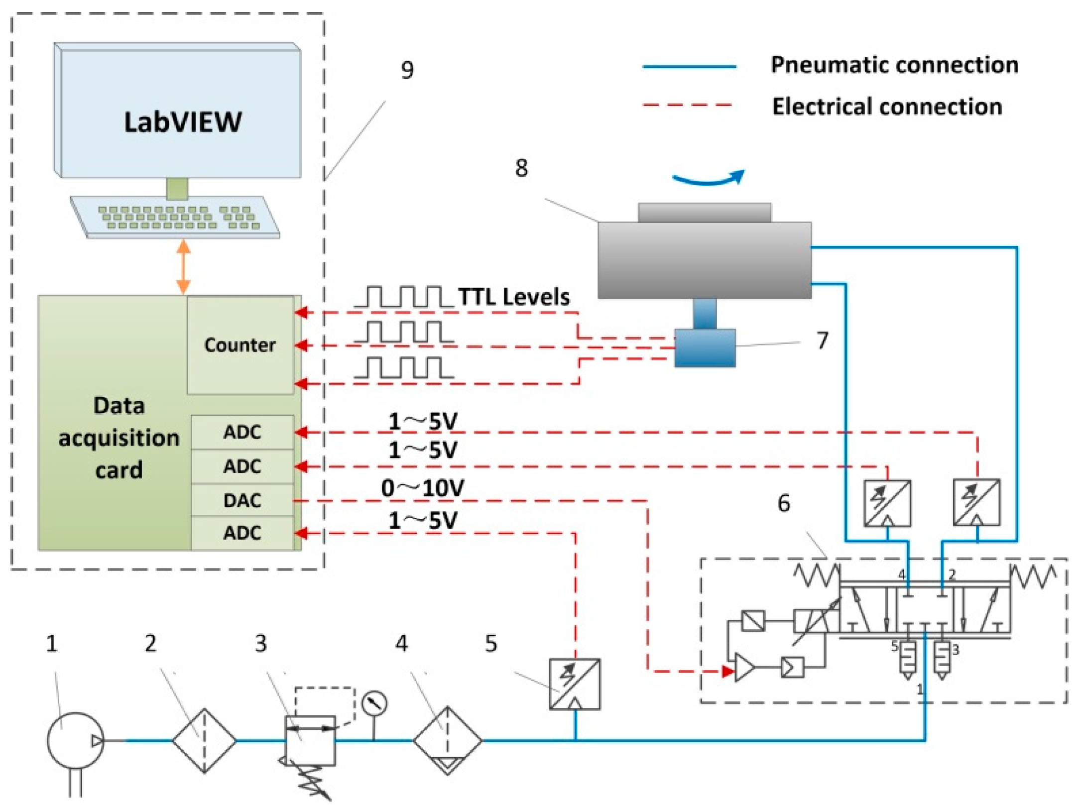
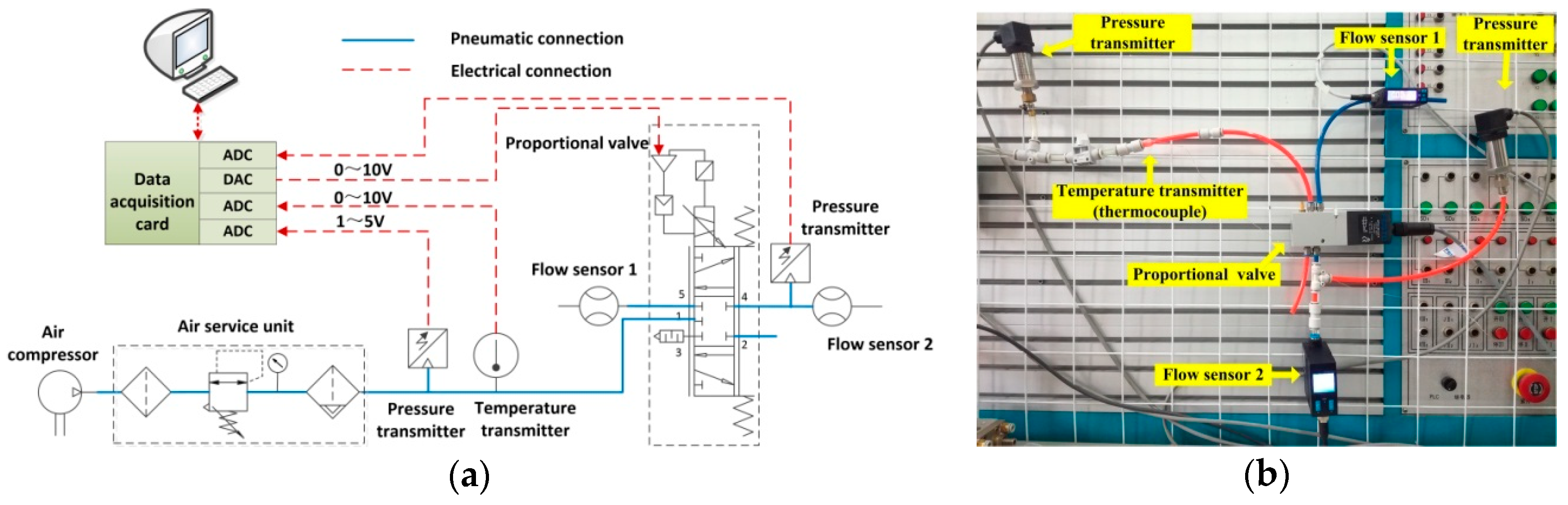
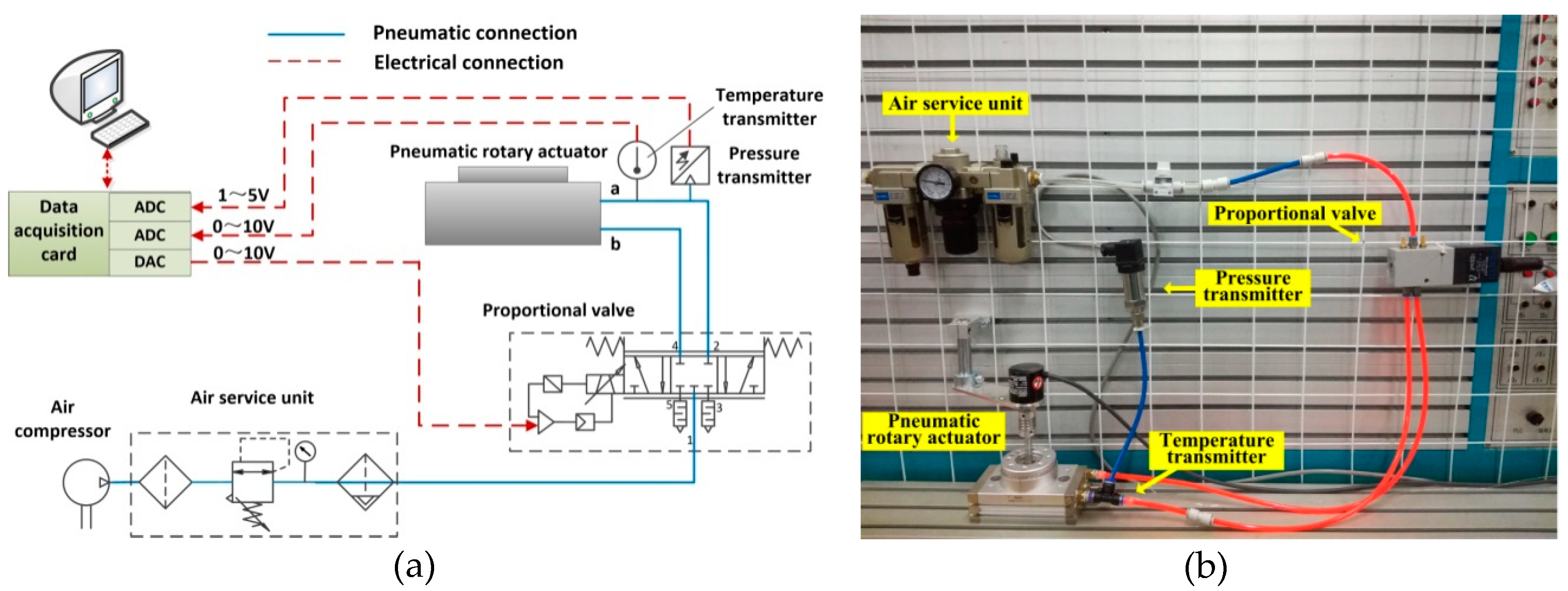
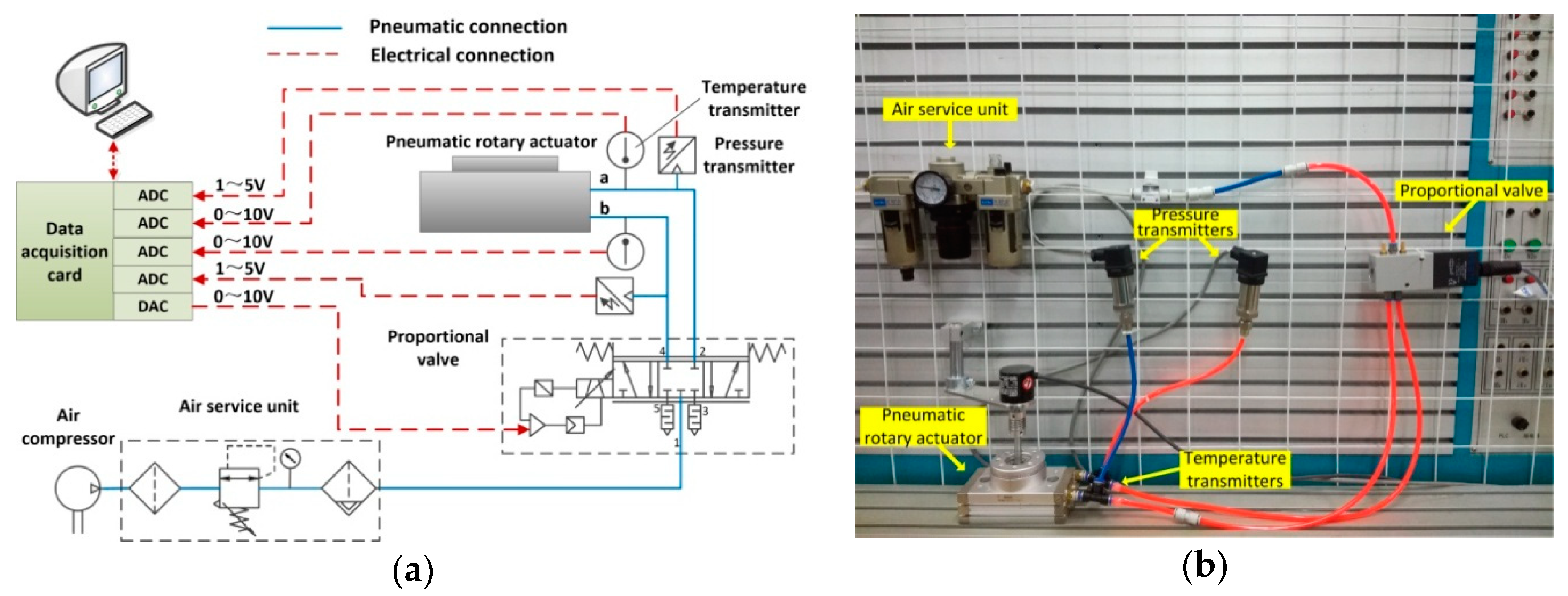
Figure 1 is the schematic diagram of a pneumatic rotary actuator position servo system, in which solid lines connect pneumatic circuits and dotted lines the electrical circuits. The compressed air produced by an air compressor is filtered and decompressed by an air service unit (air filter, air regulator and air lubricator) to provide a stable pressure for the system. A 5/3-way proportional directional control valve is used as the control valve of the system. The rotation angle of the pneumatic rotary actuator is measured by a rotary encoder, and the transistor-to-transistor logic (TTL) levels generated by the rotary encoder are transmitted to the counter in the data acquisition card. At the same time, the air supply pressure and two-chamber pressures are measured by pressure transmitters which generate 1–5 V voltage signals to the data acquisition card. The industrial personal computer (IPC) is composed of a data acquisition card and a host computer based on LabVIEW. The data acquisition card can process voltage signals and TTL levels through a controller compiled by Simulink, and generate 0–10 V voltage signals to the proportional directional control valve. With the collecting and processing of signals, flow values and flow directions of the two valve ports can be changed to accurately control the rotation angle of the pneumatic rotary actuator.

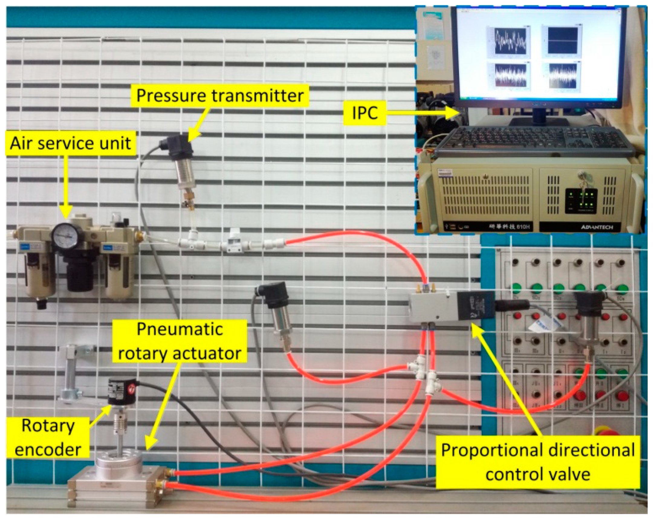
Figure 2 is the experimental platform of the pneumatic rotary actuator position servo system. The pneumatic rotary actuator is fixed on the horizontal rail and the proportional direction control valve is parallel to the horizontal plane. The models and parameters of main components are listed in

Table 1. Models and parameters of main components.

No.	Component	Model	Parameter
1	Air compressor	PANDA 750-30L	Maximum supply pressure: 0.8 MPa
2	Air service unit	AC3000-03	Maximum working pressure: 1.0 MPa
3	Pressure transmitter	CYYZ11	Range: 0–0.6 MPa; accuracy: 0.1% FS
4	Proportional direction control valve	FESTO MPYE-5-M5-010-B	Rated flow rate: 100 L/min
5	Rotary encoder	GSS06-LDH-RAG20000Z1	Resolution: 20,000 P/R
6	Pneumatic rotary actuator	SMC MSQA30A	Bore: 30 mm; stroke: 190 °
7	Data acquisition card	NI PCI-6229	32-channel analog input; 4-channel analog output; 32-bit counter
	IPC	IPC-610H	32-bit processor; standard configuration

.

3. Mass Flow Rates of the Proportional Direction Control Valve

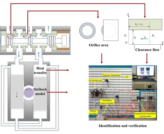
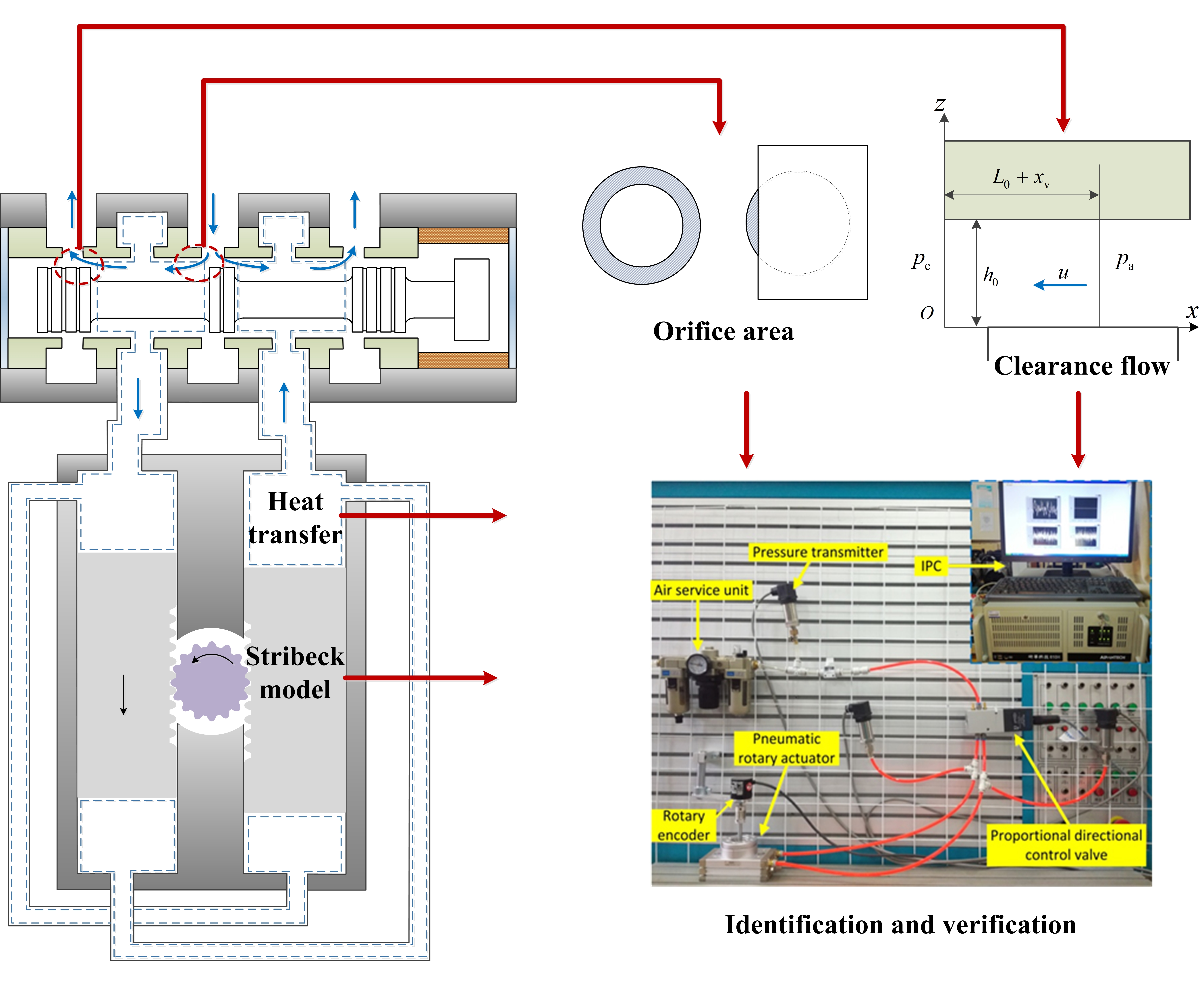
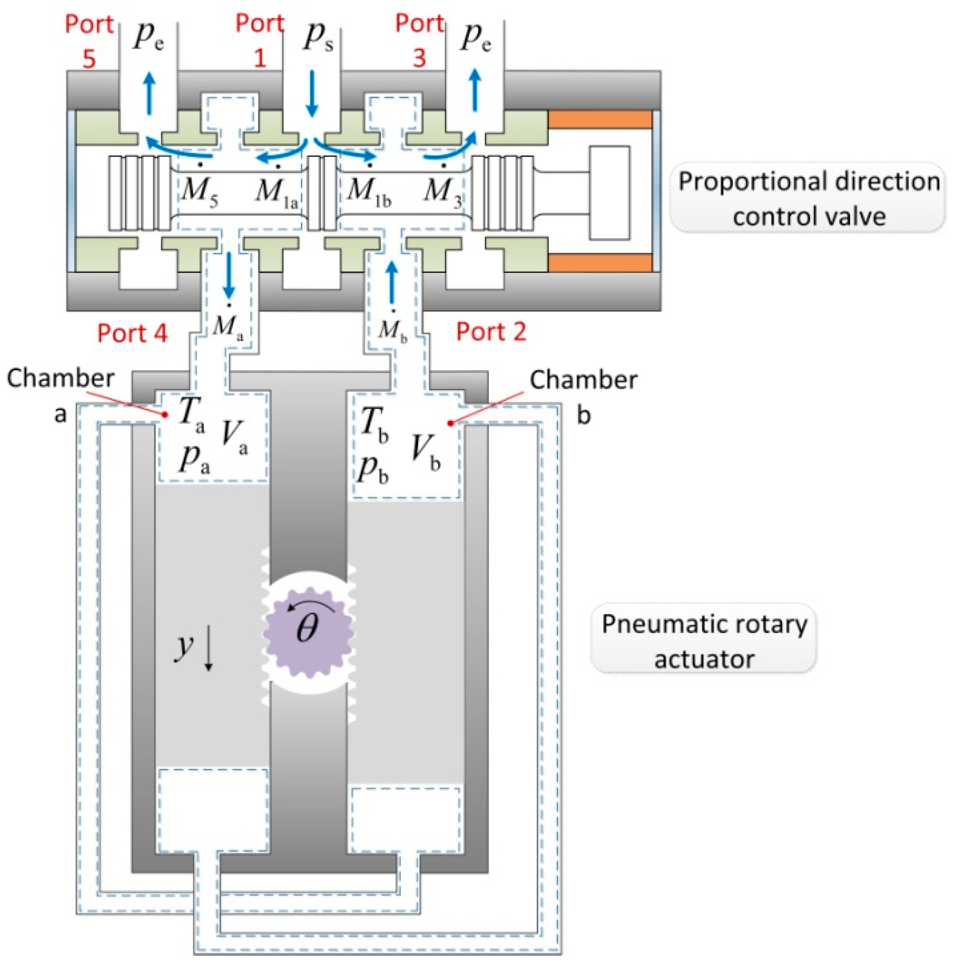
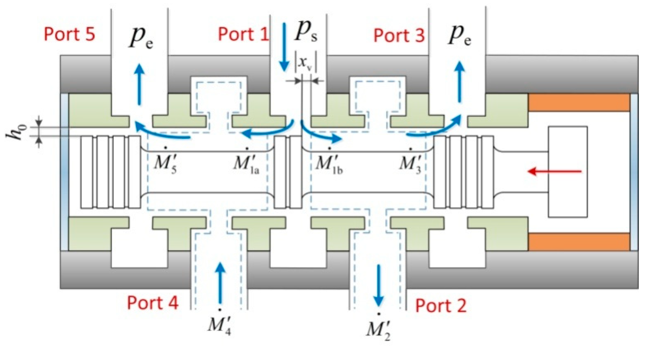
As shown in Figure 3, the right and left chambers of the proportional directional control valve are respectively connected to the two chambers of the pneumatic rotary actuator, and the air flow between them is unimpeded. Therefore, one of the proportional valve chambers and the connected actuator chamber can be regarded as a common whole which is also known as a control body where the gas temperature and pressure are evenly distributed, and the control bodies are represented by dashed lines. We can set the left control body as chamber a, and another control body chamber b.

The movement of the proportional direction control valve will generate clearance or an orifice at each valve port. At port 1, because of the existence of clearance, the gas will flow to the left chamber and the right chamber at the same time. In most studies, the gas flow generated by the clearance is often neglected, which also affects the control accuracy of the system. Therefore, we derive the mass flow rates of the gas flowing through clearance and the orifice, respectively, to make the model more accurate.

3.1. Gas Flow Mechanism in the Proportional Direction Control Valve

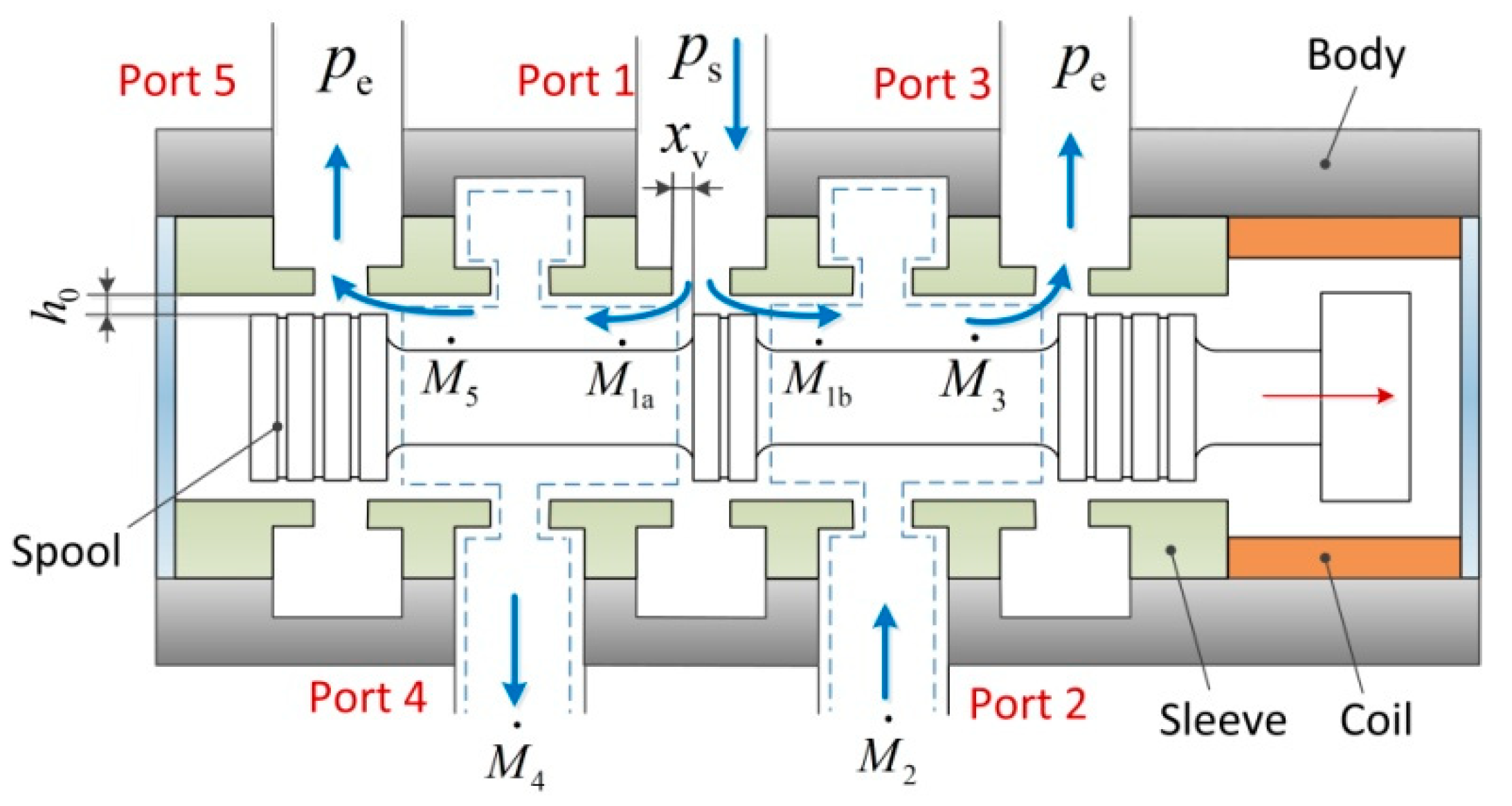
It is assumed that the direction of the proportional valve moving to the right is the positive direction, then the displacement of the spool is positive, and $x_{\mathrm{v}}>0$. As shown in Figure 4, for the left chamber, the movement of the spool makes port 5 a clearance and port 1 a throttle. For the right chamber, port 1 forms a clearance, and port 3 a throttle. At port 1, most of the gas flows through the orifice to the left chamber, and a small portion of the gas flows through the clearance to the right chamber.

The gas flow process of the left chamber is that the compressed air at port 1 flows through the orifice and then into the left chamber; the gas in the left chamber flows through the clearance of port 5 and then into the atmosphere. Since the volume of the proportional valve chamber is much smaller than that of the actuator chamber, the mass change rate $\stackrel{.}{M_{\mathrm{a}}}$ of the gas in chamber a is equal to the mass flow rate $\stackrel{.}{M_4}$ at port 4, which can be expressed by Equation (1).

$$\stackrel{.}{M_{\mathrm{a}}}=\stackrel{.}{M_4}=\stackrel{.}{M_{1\mathrm{a}}}-\stackrel{.}{M_5},$$

(1)

where $\stackrel{.}{M_{1\mathrm{a}}}$ is the mass flow rate of the gas flowing from port 1 to chamber a, and $\stackrel{.}{M_5}$ is the mass flow rate of the gas flowing through port 5.

The gas flow process of the right chamber is that the compressed air at port 1 flows through the clearance and then into the right chamber; the gas in the right chamber flows through the orifice of port 3 and then into the atmosphere. The mass change rate $\stackrel{.}{M_{\mathrm{b}}}$ of the gas in chamber b is equal to the mass flow rate $\stackrel{.}{M_2}$ at port 2, and can be expressed by Equation (2).

$$\stackrel{.}{M_{\mathrm{b}}}=\stackrel{.}{M_2}=\stackrel{.}{M_{1\mathrm{b}}}-\stackrel{.}{M_3},$$

(2)

where $\stackrel{.}{M_{1\mathrm{b}}}$ is the mass flow rate of the gas flowing from port 1 to chamber b, and $\stackrel{.}{M_3}$ is the mass flow rate of the gas flowing through port 3.

3.2. Mass Flow Rates of the Gas Flowing through the Orifices

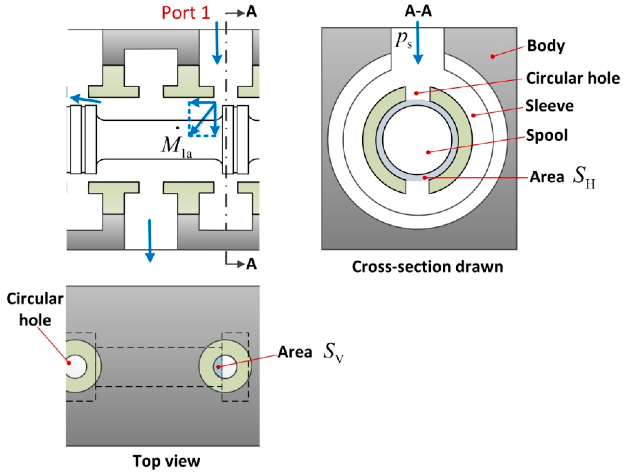
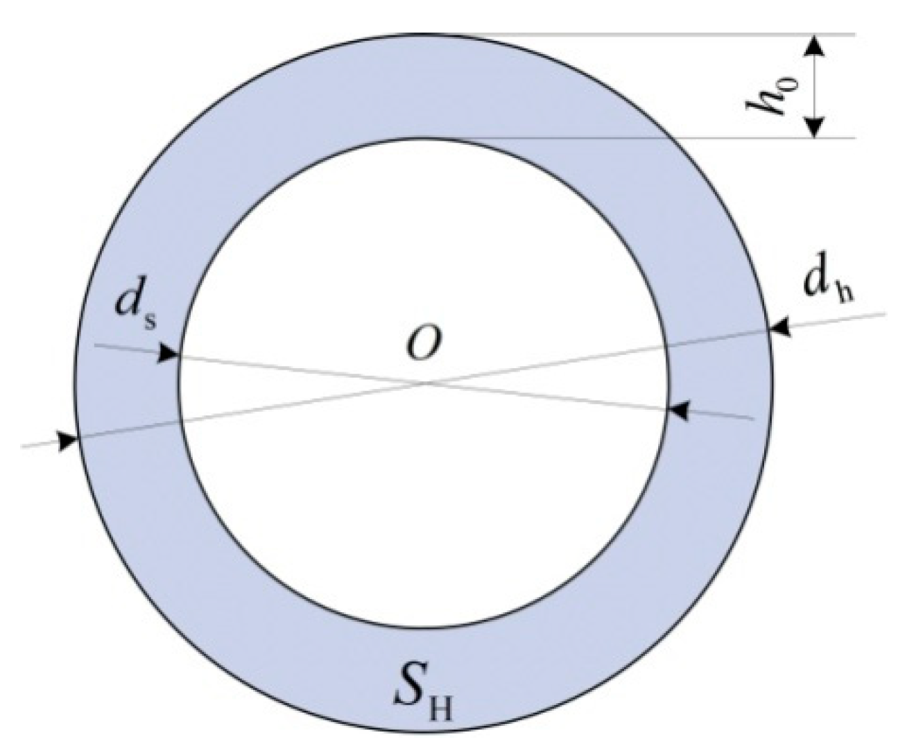
In Figure 5, the sleeve of the proportional valve has two symmetrical circular holes in the same vertical direction. The gas flows through both two circular holes into chambers or the atmosphere. When the spool moves to the right, the spool shoulder covers two holes to form the two same orifices in the same vertical direction.

In Figure 5, because of the existence of the clearance, the mass flow rate $\stackrel{.}{M_{1\mathrm{a}}}$ can be regarded as the scaled value of two mass flow rates in the horizontal and vertical directions. Correspondingly, the orifice has a physical area in each direction. The shadow area $S_{\mathrm{V}}$ represents the physical area of the orifice in the vertical direction and the shadow area $S_{\mathrm{H}}$ represents the physical area of the orifice in the horizontal direction. The effective area $S_{\mathrm{e}}$ of the orifice can be assumed as follows:

$$S_{\mathrm{e}}=C_1\left(2S_{\mathrm{V}}+C_0{S}_{\mathrm{H}}\right)=2C_1{S}_{\mathrm{V}}+C_0{C}_1{S}_{\mathrm{H}},$$

(3)

where $C_1$ is the flow coefficient of the orifice, which is necessary because there is pressure loss when the gas passes through the orifice; $2S_{\mathrm{V}}+C_0{S}_{\mathrm{H}}$ represents the physical area of the orifice; and $C_0$ is an assumed coefficient to realize the area conversion from horizontal direction to vertical direction. Both $S_{\mathrm{V}}$ and $S_{\mathrm{H}}$ can be obtained by calculation. Even if the spool displacement is changed, the clearance area and shape in the horizontal direction are constant. Therefore, the influence of $S_{\mathrm{H}}$ on $S_{\mathrm{V}}$ can be regarded as constant, that is, $C_0$ can be regarded as a fixed value. When the spool is in the middle position, $S_{\mathrm{e}}=C_0{C}_1{S}_{\mathrm{H}}$. After that, the value of $C_0{C}_1$ can be solved. Substituting the value of $C_0{C}_1$ into Equation (3) yields the value of $C_1$, and then $C_0$ can be obtained. However, $C_1$ changes with the position of the spool, and the expression of $C_1$ can be obtained by test.

In addition, the effective area of the orifice at port 3 is equal to the effective area of the orifice at port 1.

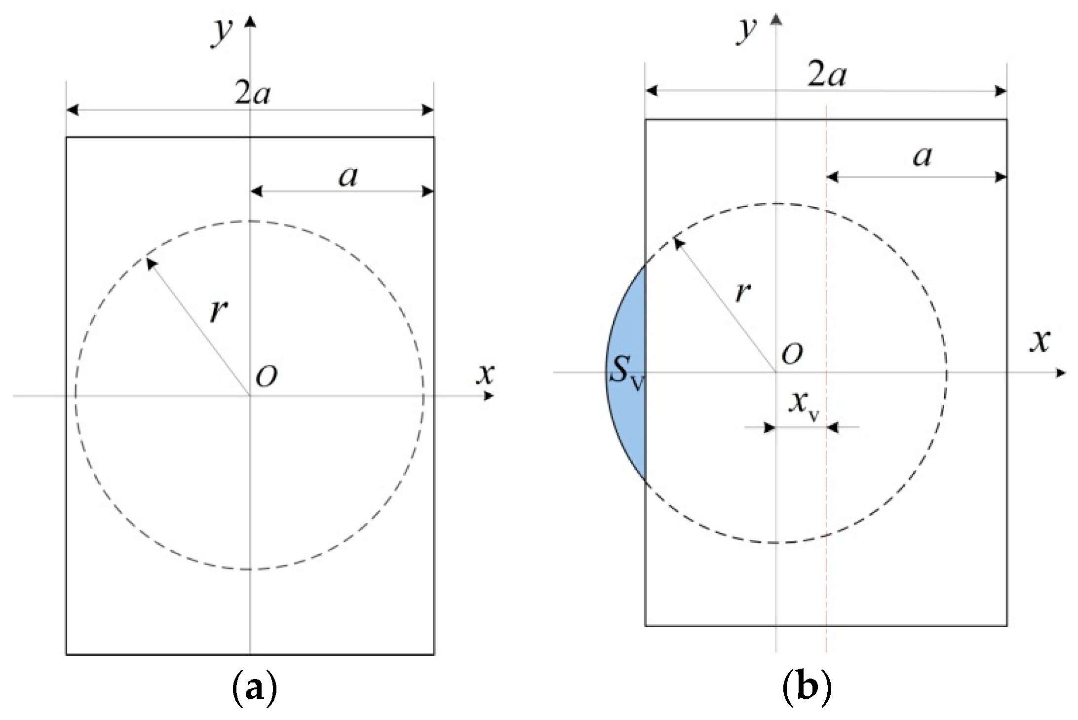
Figure 6a shows the relative position of the circular hole and the spool shoulder when the proportional valve spool is in the initial position. Figure 6b shows the relative position when the displacement of the spool is $x_{\mathrm{v}}$. Moreover, circle center $O$ is the origin of the coordinate. $r$ is the radius of the circular hole. $x_{\mathrm{v}}$ represents the displacement of the spool, and the width of the spool shoulder is $2a$.

Then, we can obtain the physical area $S_{\mathrm{V}}$ from their geometric relations.

$$S_{\mathrm{V}}=\{\begin{array}{ll}0& x_{\mathrm{v}}\le a-r\\ r^2\arccos \frac{a-x_{\mathrm{v}}}{r}-\left(a-x_{\mathrm{v}}\right)\sqrt{r^2-{\left(a-x_{\mathrm{v}}\right)}^2}& a-r<x_{\mathrm{v}}\le a\end{array}.$$

(4)

Figure 7 shows the physical area of the orifice in the horizontal direction, where $h_0$ represents the length of the clearance, $d_{\mathrm{s}}$ is the diameter of the spool shoulder, and $d_{\mathrm{h}}$ represents the inner diameter of the sleeve. It is easy to obtain Equations (5) and (6):

$$S_{\mathrm{H}}=\frac{\pi \left(d_{\mathrm{h}}^2-d_{\mathrm{s}}^2\right)}{4},$$

(5)

$$h_0=\frac{d_{\mathrm{h}}-d_{\mathrm{s}}}{2}.$$

(6)

Therefore, the effective area of the orifice can be obtained by Equations (3)–(5).

$$S_{\mathrm{e}}=\{\begin{array}{ll}\frac{C_1{C}_0\pi \left(d_{\mathrm{h}}^2-d_{\mathrm{s}}^2\right)}{4}& 0\le x_{\mathrm{v}}\le a-r\\ C_1\left[2r^2\arccos \frac{a-x_{\mathrm{v}}}{r}-2\left(a-x_{\mathrm{v}}\right)\sqrt{r^2-{\left(a-x_{\mathrm{v}}\right)}^2}+\frac{C_0\pi \left(d_{\mathrm{h}}^2-d_{\mathrm{s}}^2\right)}{4}\right]& a-r<x_{\mathrm{v}}\le a\end{array}.$$

(7)

It is assumed that the gas flowing through the orifice has no time to exchange heat with the outside and has no friction loss, hence it can be considered as an isentropic adiabatic process [21]. According to the research by Sanville. F. E. [22], the mass flow rates of the gas flowing through the orifices can be described by the following equations.

$$\stackrel{.}{M_{1\mathrm{a}}}=\{\begin{array}{ll}\frac{S_{\mathrm{e}}{p}_{\mathrm{s}}}{\sqrt{R{T}_{\mathrm{s}}}}\sqrt{\frac{2\kappa }{\kappa -1}\left[{\left(\frac{p_{\mathrm{a}}}{p_{\mathrm{s}}}\right)}^{\frac{2}{\kappa }}-{\left(\frac{p_{\mathrm{a}}}{p_{\mathrm{s}}}\right)}^{\frac{\kappa +1}{\kappa }}\right]}& \left(\frac{p_{\mathrm{a}}}{p_{\mathrm{s}}}\ge b\right)\\ \frac{S_{\mathrm{e}}{p}_{\mathrm{s}}}{\sqrt{R{T}_{\mathrm{s}}}}\sqrt{\frac{2\kappa }{\kappa +1}{\left(\frac{2}{\kappa +1}\right)}^{\frac{2}{\kappa -1}}}& \left(\frac{p_{\mathrm{a}}}{p_{\mathrm{s}}}<b\right)\end{array},$$

(8)

$$\stackrel{.}{M_3}=\{\begin{array}{ll}\frac{S_{\mathrm{e}}{p}_{\mathrm{b}}}{\sqrt{R{T}_{\mathrm{b}}}}\sqrt{\frac{2\kappa }{\kappa -1}\left[{\left(\frac{p_{\mathrm{e}}}{p_{\mathrm{b}}}\right)}^{\frac{2}{k}}-{\left(\frac{p_{\mathrm{e}}}{p_{\mathrm{b}}}\right)}^{\frac{\kappa +1}{\kappa }}\right]}& \left(\frac{p_{\mathrm{e}}}{p_{\mathrm{b}}}\ge b\right)\\ \frac{S_{\mathrm{e}}{p}_{\mathrm{b}}}{\sqrt{R{T}_{\mathrm{b}}}}\sqrt{\frac{2\kappa }{\kappa +1}{\left(\frac{2}{\kappa +1}\right)}^{\frac{2}{\kappa -1}}}& \left(\frac{p_{\mathrm{e}}}{p_{\mathrm{b}}}<b\right)\end{array},$$

(9)

where $p_{\mathrm{s}}$ is the supply pressure, $p_{\mathrm{a}}$ and $p_{\mathrm{b}}$ represent the pressures of chamber a and b, respectively, and $p_{\mathrm{e}}$ is atmospheric pressure. $T_{\mathrm{s}}$ represents the supply temperature, $T_{\mathrm{b}}$ represents the temperature of the gas in chamber b, $R$ is the gas constant, $b$ is the critical pressure ratio, and $\kappa$ is isentropic index. The isentropic index exists in the isentropic process and is equal to the ratio of the heat capacity at constant pressure to heat capacity at constant volume. The isentropic index of air at room temperature is 1.4.

3.3. Mass Flow Rates of the Gas Flowing through the Clearances

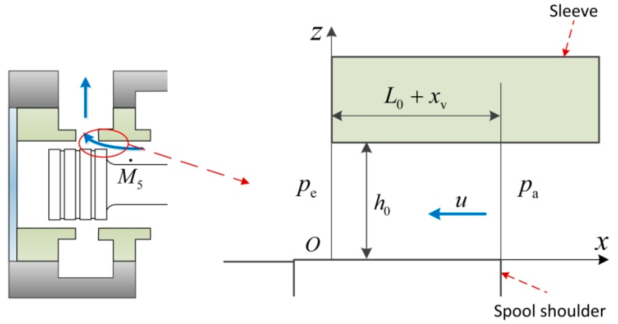
The flow of the gas flowing through the clearance is similar to the flow of viscous fluid between the parallel plates [23]. Figure 8 is the schematic diagram of the clearance flow at port 5, when the spool moves to the right. The initial length of the clearance is $L_0$. Referring to the equation of the clearance flow between two parallel plates, we can get the differential equation of the gas pressure.

$$\frac{\mathrm{d}p}{\mathrm{d}x}=-\mu \frac{{\mathrm{d}}^{2}u}{\mathrm{d}{z}^2},$$

(10)

where $p$ is the pressure of the gas micelle in the clearance, $\mu$ is the viscosity coefficient of the gas, and $u$ is the velocity of the gas micelles in the horizontal direction.

The boundary conditions are:

$$\{\begin{array}{ll}\mathrm{when}z=0,& u=0\\ \mathrm{when}z=h_0,& u=0\end{array}$$

(11)

and

$$\{\begin{array}{ll}\mathrm{when}x=0,& p=p_{\mathrm{e}}\\ \mathrm{when}x=L_0+x_{\mathrm{v}},& p=p_{\mathrm{a}}\end{array}.$$

(12)

According to the boundary condition Equation (11), the equation of the airflow velocity varying with $\mathrm{d}p/\mathrm{d}x$ can be obtained by solving Equation (10).

$$u=-\frac{1}{2\mu }\frac{\mathrm{d}p}{\mathrm{d}x}z\left(z-h_0\right).$$

(13)

The mass flow rate of the gas flowing through the clearance is

$$\stackrel{.}{M_5}={\rho }_{\mathrm{e}}{\displaystyle {\int }_0^{h_0}u·\pi d_{\mathrm{s}}\mathrm{d}z},$$

(14)

where ${\rho }_{\mathrm{e}}$ is atmospheric density.

The size of the plate clearance is constant in the direction of the $x$ axis, so the change rate of $p$ along the $x$ axis decreases uniformly. Therefore, combined with the boundary condition Equation (12),

$$\frac{\mathrm{d}p}{\mathrm{d}x}=\frac{p_{\mathrm{a}}-p_{\mathrm{e}}}{L_0+x_{\mathrm{v}}}.$$

(15)

The ideal gas law is $p/\rho =RT$, where $\rho$ is gas density, and $T$ is gas temperature. The gas velocity in the clearance is very low, and the gas exchanges heat with the outside sufficiently. Hence, the state change of the gas in the clearance can be regarded approximately as an isothermal process:

$${\rho }_e=\frac{p_{\mathrm{e}}}{R{T}_{\mathrm{a}}}.$$

(16)

After substituting Equations (6), (13), (15) and (16) into Equation (14), we obtain

$$\stackrel{.}{M_5}=\frac{p_{\mathrm{e}}}{R{T}_{\mathrm{a}}}{\displaystyle {\int }_0^{h_0}-\frac{1}{2\mu }·\frac{p_{\mathrm{a}}-p_{\mathrm{e}}}{L_0+x_{\mathrm{v}}}·z\left(z-h_0\right)·\pi d_{\mathrm{s}}\mathrm{d}z}=\frac{\pi d_{\mathrm{s}}{h}_0^3{p}_{\mathrm{e}}\left(p_{\mathrm{a}}-p_{\mathrm{e}}\right)}{12\mu \left(L_0+x_{\mathrm{v}}\right)R{T}_{\mathrm{a}}}=\frac{\pi d_{\mathrm{s}}{\left(d_{\mathrm{h}}-d_{\mathrm{s}}\right)}^3{p}_{\mathrm{e}}\left(p_{\mathrm{a}}-p_{\mathrm{e}}\right)}{96\mu \left(L_0+x_{\mathrm{v}}\right)R{T}_{\mathrm{a}}}$$

(17)

Similarly, the mass flow rate $\stackrel{.}{M_{1\mathrm{b}}}$ can also be obtained using the above principle.

$$\stackrel{.}{M_{1\mathrm{b}}}=\frac{\pi d_{\mathrm{s}}{\left(d_{\mathrm{h}}-d_{\mathrm{s}}\right)}^3{p}_{\mathrm{b}}\left(p_{\mathrm{s}}-p_{\mathrm{b}}\right)}{96\mu \left(L_0+x_{\mathrm{v}}\right)R{T}_{\mathrm{s}}}.$$

(18)

3.4. Mass Flow Rates When the Spool Moves Backward

When the spool moves to the left, $x_{\mathrm{v}}<0$. As shown in Figure 9, the gas flowing from port 1 to the right chamber and the gas flowing from the left chamber to atmosphere are throttled flow. The gas flowing from port 1 to the left chamber and the gas flowing from the right chamber to the atmosphere are clearance flow. Their mass flow rates are represented by $\stackrel{.}{M_5^{\prime }}$, $\stackrel{.}{M_{1\mathrm{a}}^{\prime }}$, $\stackrel{.}{M_{\mathrm{a}}^{\prime }}$, $\stackrel{.}{M_{1\mathrm{b}}^{\prime }}$, $\stackrel{.}{M_{\mathrm{b}}^{\prime }}$ and $\stackrel{.}{M_3^{\prime }}$, respectively, and they still have the following relationships.

$$\stackrel{.}{M_{\mathrm{a}}^{\prime }}=\stackrel{.}{M_{1\mathrm{a}}^{\prime }}-\stackrel{.}{M_5^{\prime }},$$

(19)

$$\stackrel{.}{M_{\mathrm{b}}^{\prime }}=\stackrel{.}{M_{1\mathrm{b}}^{\prime }}-\stackrel{.}{M_3^{\prime }}.$$

(20)

The physical area of the orifice can be expressed as

$$S_{\mathrm{e}}^{\prime }=\{\begin{array}{ll}{C}_1\left[2r^2\arccos \frac{a+x_{\mathrm{v}}}{r}-2\left(a+x_{\mathrm{v}}\right)\sqrt{r^2-{\left(a+x_{\mathrm{v}}\right)}^2}+\frac{C_0\pi \left(d_{\mathrm{h}}^2-d_{\mathrm{s}}^2\right)}{4}\right]& -a\le x_{\mathrm{v}}<r-a\\ \frac{C_1{C}_0\pi \left(d_{\mathrm{h}}^2-d_{\mathrm{s}}^2\right)}{4}& r-a\le x_{\mathrm{v}}<0\end{array}.$$

(21)

The mass flow rates of the gas flowing through the orifices can be rewritten as

$$\stackrel{.}{M_5^{\prime }}=\{\begin{array}{ll}\frac{S_{\mathrm{e}}^{\prime }{p}_{\mathrm{a}}}{\sqrt{R{T}_{\mathrm{a}}}}\sqrt{\frac{2\kappa }{\kappa -1}\left[{\left(\frac{p_{\mathrm{e}}}{p_{\mathrm{a}}}\right)}^{\frac{2}{\kappa }}-{\left(\frac{p_{\mathrm{e}}}{p_{\mathrm{a}}}\right)}^{\frac{\kappa +1}{\kappa }}\right]}& \left(\frac{p_{\mathrm{e}}}{p_{\mathrm{a}}}\ge b\right)\\ \frac{S_{\mathrm{e}}^{\prime }{p}_{\mathrm{a}}}{\sqrt{R{T}_{\mathrm{a}}}}\sqrt{\frac{2\kappa }{\kappa +1}{\left(\frac{2}{\kappa +1}\right)}^{\frac{2}{\kappa -1}}}& \left(\frac{p_{\mathrm{e}}}{p_{\mathrm{a}}}<b\right)\end{array},$$

(22)

$$\stackrel{.}{M_{1\mathrm{b}}^{\prime }}=\{\begin{array}{ll}\frac{S_{\mathrm{e}}^{\prime }{p}_{\mathrm{s}}}{\sqrt{R{T}_{\mathrm{s}}}}\sqrt{\frac{2\kappa }{\kappa -1}\left[{\left(\frac{p_{\mathrm{b}}}{p_{\mathrm{s}}}\right)}^{\frac{2}{\kappa }}-{\left(\frac{p_{\mathrm{b}}}{p_{\mathrm{s}}}\right)}^{\frac{\kappa +1}{\kappa }}\right]}& \left(\frac{p_{\mathrm{b}}}{p_{\mathrm{s}}}\ge b\right)\\ \frac{S_{\mathrm{e}}^{\prime }{p}_{\mathrm{s}}}{\sqrt{R{T}_{\mathrm{s}}}}\sqrt{\frac{2\kappa }{\kappa +1}{\left(\frac{2}{\kappa +1}\right)}^{\frac{2}{\kappa -1}}}& \left(\frac{p_{\mathrm{b}}}{p_{\mathrm{s}}}<b\right)\end{array},$$

(23)

where $T_{\mathrm{a}}$ is the temperature of the gas in chamber a.

The mass flow rates of the gas flowing through the clearances are as follows:

$$\stackrel{.}{M_{1\mathrm{a}}^{\prime }}=\frac{\pi d_{\mathrm{s}}{\left(d_{\mathrm{h}}-d_{\mathrm{s}}\right)}^3{p}_{\mathrm{a}}\left(p_{\mathrm{s}}-p_{\mathrm{a}}\right)}{96\mu \left(L_0-x_{\mathrm{v}}\right)R{T}_{\mathrm{s}}},$$

(24)

$$\stackrel{.}{M_3^{\prime }}=\frac{\pi d_{\mathrm{s}}{\left(d_{\mathrm{h}}-d_{\mathrm{s}}\right)}^3{p}_{\mathrm{e}}\left(p_{\mathrm{b}}-p_{\mathrm{e}}\right)}{96\mu \left(L_0-x_{\mathrm{v}}\right)R{T}_{\mathrm{b}}}.$$

(25)

4. Non-linear Model of the Valve-Controlled Actuator System

As shown in Figure 3, the compressed air flows into two chambers through the proportional valve, and the gas of two chambers is deflated to the outside at the same time. With the influence of the pressures ($p_{\mathrm{a}}$,$p_{\mathrm{b}}$) and the external heat transfer, the actuator piston overcomes the external forces and moves. The rectilinear motion of the actuator piston is converted into the rotary motion of the gear by the inter-tooth meshing transmission. The non-linear model of the pneumatic rotary actuator can be expressed by the energy equation, pressure differential equation and dynamic model.

4.1. Energy Equation

Gas flow will change the gas temperature, which will also affect the gas pressure and actuator rotation angle. The energy equation can make the model better describe the change regulation of the gas temperature and improve the accuracy of the model. The energy equation can be derived from the first law of thermodynamics, and the heat transfer formula needs to be taken into account.

Within the time $\mathrm{d}t$, the first law of thermodynamics can be written as

$$\mathrm{d}U+\mathrm{d}W=\mathrm{d}H+\mathrm{d}Q,$$

(26)

where $U$ is the thermodynamic energy change in a chamber, $W$ is the work done to the outside, $H$ is the net inflow energy of the gas, and $Q$ is the gas heat given by the outside.

The thermodynamic energy change in each chamber is

$$\{\begin{array}{l}\mathrm{d}{U}_{\mathrm{a}}=\left[\left(c_V{T}_{\mathrm{a}}\right)+\mathrm{d}\left(c_V{T}_{\mathrm{a}}\right)\right]\left(m_{\mathrm{a}}+\mathrm{d}{m}_{\mathrm{a}}\right)-c_V{T}_{\mathrm{a}}{m}_{\mathrm{a}}=c_V\left(m_{\mathrm{a}}\mathrm{d}{T}_{\mathrm{a}}+T_{\mathrm{a}}\mathrm{d}{m}_{\mathrm{a}}\right)=c_V\left[m_{\mathrm{a}}\mathrm{d}{T}_{\mathrm{a}}+T_{\mathrm{a}}\left(\stackrel{.}{M_{1\mathrm{a}}}-\stackrel{.}{M_5}\right)\mathrm{d}t\right]\\ \mathrm{d}{U}_{\mathrm{b}}=\left[\left(c_V{T}_{\mathrm{b}}\right)+\mathrm{d}\left(c_V{T}_{\mathrm{b}}\right)\right]\left(m_{\mathrm{b}}+\mathrm{d}{m}_{\mathrm{b}}\right)-c_V{T}_{\mathrm{b}}{m}_{\mathrm{b}}=c_V\left(m_{\mathrm{b}}\mathrm{d}{T}_{\mathrm{b}}+T_{\mathrm{b}}\mathrm{d}{m}_{\mathrm{b}}\right)=c_V\left[m_{\mathrm{b}}\mathrm{d}{T}_{\mathrm{b}}+T_{\mathrm{b}}\left(\stackrel{.}{M_{1\mathrm{b}}}-\stackrel{.}{M_3}\right)\mathrm{d}t\right]\end{array}$$

(27)

where $c_V$ denotes the mass heat capacity at constant volume, and $c_V=R/\left(\kappa -1\right)$; $m_{\mathrm{a}}$ and $m_{\mathrm{b}}$ represent the mass of the gas in chamber a and b, respectively; and both $c_V\mathrm{d}{T}_{\mathrm{a}}\mathrm{d}{m}_{\mathrm{a}}$ and $c_V\mathrm{d}{T}_{\mathrm{b}}\mathrm{d}{m}_{\mathrm{b}}$ can be ignored.

The work done to the outside can be expressed as

$$\{\begin{array}{l}\mathrm{d}{W}_{\mathrm{a}}=2A{p}_{\mathrm{a}}dy=A{p}_{\mathrm{a}}{d}_{\mathrm{f}}d\theta \\ \mathrm{d}{W}_{\mathrm{b}}=-2A{p}_{\mathrm{b}}dy=-A{p}_{\mathrm{b}}{d}_{\mathrm{f}}d\theta \end{array},$$

(28)

where $A$ is the effective area of the actuator piston, $y$ represents the displacement of the piston, $d_{\mathrm{f}}$ is the pitch diameter of the pinion, and $\theta$ is the rotation angle of the actuator.

The net inflow energy of the gas in each chamber can be expressed as

$$\{\begin{array}{l}\mathrm{d}{H}_{\mathrm{a}}=c_p{T}_{\mathrm{s}}\mathrm{d}{m}_{1\mathrm{a}}-c_p{T}_{\mathrm{a}}\mathrm{d}{m}_5=c_p{T}_{\mathrm{s}}\stackrel{.}{M_{1\mathrm{a}}}\mathrm{d}t-c_p{T}_{\mathrm{a}}\stackrel{.}{M_5}\mathrm{d}t\\ \mathrm{d}{H}_{\mathrm{b}}=c_p{T}_{\mathrm{s}}\mathrm{d}{m}_{1\mathrm{b}}-c_p{T}_{\mathrm{b}}\mathrm{d}{m}_3=c_p{T}_{\mathrm{s}}\stackrel{.}{M_{1\mathrm{b}}}\mathrm{d}t-c_p{T}_{\mathrm{b}}\stackrel{.}{M_3}\mathrm{d}t\end{array},$$

(29)

where $c_p$ is the mass heat capacity at constant pressure, and $c_p=\kappa c_V$ and $c_p=c_V+R$. $\mathrm{d}{m}_{1\mathrm{a}}$, $\mathrm{d}{m}_5$, $\mathrm{d}{m}_{1\mathrm{b}}$ and $\mathrm{d}{m}_3$, respectively correspond to the mass of the gas flowing through each port within time $\mathrm{d}t$.

The gas heat given by the outside can be expressed by the heat transfer formula. It is assumed that the inner wall temperature of the chamber is not affected by charging or discharging, and that the temperature is equal to the room temperature $T_{\mathrm{e}}$. Therefore, the expressions of the gas heat transfer are

$$\{\begin{array}{l}\mathrm{d}{Q}_{\mathrm{a}}=h{S}_{\mathrm{ha}}(T_{\mathrm{e}}-T_{\mathrm{a}})\mathrm{d}t\\ \mathrm{d}{Q}_{\mathrm{b}}=h{S}_{\mathrm{hb}}(T_{\mathrm{e}}-T_{\mathrm{b}})\mathrm{d}t\end{array},$$

(30)

where $h$ is the heat transfer coefficient between the gas and the inner wall of two chambers. $S_{\mathrm{ha}}$ and $S_{\mathrm{hb}}$ are the inner wall areas of two respective chambers.

After substituting Equations (27)–(30) into Equation (26), we can obtain the final expressions of the energy equation.

$$\{\begin{array}{l}\frac{c_V{p}_{\mathrm{a}}{V}_{\mathrm{a}}}{R{T}_{\mathrm{a}}}\frac{\mathrm{d}{T}_{\mathrm{a}}}{\mathrm{d}t}=c_V\left(\kappa T_{\mathrm{s}}-T_{\mathrm{a}}\right)\stackrel{.}{M_{1\mathrm{a}}}-R{T}_{\mathrm{a}}\stackrel{.}{M_5}-A{p}_{\mathrm{a}}{d}_{\mathrm{f}}\frac{\mathrm{d}\theta }{\mathrm{d}t}+h{S}_{\mathrm{ha}}\left(T_{\mathrm{e}}-T_{\mathrm{a}}\right)\\ \frac{c_V{p}_{\mathrm{b}}{V}_{\mathrm{b}}}{R{T}_{\mathrm{b}}}\frac{\mathrm{d}{T}_{\mathrm{b}}}{\mathrm{d}t}=c_V\left(\kappa T_{\mathrm{s}}-T_{\mathrm{b}}\right)\stackrel{.}{M_{1\mathrm{b}}}-R{T}_{\mathrm{b}}\stackrel{.}{M_3}+A{p}_{\mathrm{b}}{d}_{\mathrm{f}}\frac{\mathrm{d}\theta }{\mathrm{d}t}+h{S}_{\mathrm{hb}}\left(T_{\mathrm{e}}-T_{\mathrm{b}}\right)\end{array}.$$

(31)

4.2. Pressure Differential Equation

After differentiating and simplifying the ideal gas law $pV=mRT$, we can get the pressure differential equation:

$$\{\begin{array}{l}\frac{\mathrm{d}{p}_{\mathrm{a}}}{\mathrm{d}t}=\frac{1}{V_{\mathrm{a}}}\left[R{T}_{\mathrm{a}}\left(\stackrel{.}{M_{1\mathrm{a}}}-\stackrel{.}{M_5}\right)+\frac{p_{\mathrm{a}}{V}_{\mathrm{a}}}{T_{\mathrm{a}}}\frac{\mathrm{d}{T}_{\mathrm{a}}}{\mathrm{d}t}-A{p}_{\mathrm{a}}{d}_{\mathrm{f}}\frac{\mathrm{d}\theta }{\mathrm{d}t}\right]\\ \frac{\mathrm{d}{p}_{\mathrm{b}}}{\mathrm{d}t}=\frac{1}{V_{\mathrm{b}}}\left[R{T}_{\mathrm{b}}\left(\stackrel{.}{M_{1\mathrm{b}}}-\stackrel{.}{M_3}\right)+\frac{p_{\mathrm{b}}{V}_{\mathrm{b}}}{T_{\mathrm{b}}}\frac{\mathrm{d}{T}_{\mathrm{b}}}{\mathrm{d}t}+A{p}_{\mathrm{b}}{d}_{\mathrm{f}}\frac{\mathrm{d}\theta }{\mathrm{d}t}\right]\end{array},$$

(32)

and

$$\{\begin{array}{l}{V}_{\mathrm{a}}=V_{\mathrm{a}0}+Ay=V_{\mathrm{a}0}+\frac{d_{\mathrm{f}}}{2}A\theta \\ V_{\mathrm{b}}=V_{\mathrm{b}0}-Ay=V_{\mathrm{b}0}-\frac{d_{\mathrm{f}}}{2}A\theta \end{array},$$

(33)

where $V_{\mathrm{a}0}$ is the initial volume of chamber a, and $V_{\mathrm{b}0}$ is the initial volume of chamber b.

4.3. Dynamic Model

The actuator friction mainly exists between the piston and the inner wall, and it can be divided into static friction and dynamical friction. When the piston is in the zero speed range, it is subjected to static friction force. When the piston starts to move, the piston is also affected by Coulomb friction force and viscous friction force, and part of the static friction force is replaced by dynamic friction force. Therefore, the actuator friction will decrease sharply in the beginning, and increase gradually after reaching a certain speed. The Stribeck model can accurately represent the changing trend of friction force and can smoothly connect the curves of static friction force and dynamic friction force [24]. Therefore, the Stribeck model can be used in the dynamic model of the system in this paper. The Stribeck model can be expressed by Equations (34)–(36).

When $\left|\dot{\theta }\right|\le \alpha$, the static friction force is

$$F_{\mathrm{f}}=\{\begin{array}{ll}{F}_{\mathrm{s}}& F_{\mathrm{p}}>F_{\mathrm{s}}\\ F_{\mathrm{p}}& -F_{\mathrm{s}}<F_{\mathrm{p}}<F_{\mathrm{s}}\\ -F_{\mathrm{s}}& F_{\mathrm{p}}<-F_{\mathrm{s}}\end{array},$$

(34)

where

$$F_{\mathrm{p}}=2A\left(p_{\mathrm{a}}-p_{\mathrm{b}}\right).$$

(35)

When $\left|\dot{\theta }\right|>\alpha$, the dynamic friction force is

$$F_{\mathrm{f}}=F_{\mathrm{c}}\mathrm{sgn}\left(\dot{\theta }\right)+(F_{\mathrm{s}}-F_{\mathrm{c}})e^{-{\left(\dot{\theta }/{\dot{\theta }}_{\mathrm{s}}\right)}^2}\mathrm{sgn}\left(\dot{\theta }\right)+B\dot{\theta },$$

(36)

where $\alpha$ is a small positive constant, $F_{\mathrm{s}}$ is the maximum static friction force, $F_{\mathrm{p}}$ is the driving force for the piston, $F_{\mathrm{c}}$ is Coulomb friction force,$\dot{\theta }$ is the angular velocity of the actuator, ${\dot{\theta }}_{\mathrm{s}}$ is the Stribeck speed, and $B$ is the viscous friction coefficient.

According to Newton’s second law, the moment balance equation of the actuator can be expressed as

$$A{d}_{\mathrm{f}}\left(p_{\mathrm{a}}-p_{\mathrm{b}}\right)=\left(\frac{1}{2}{m}_{\mathrm{p}}{d}_{\mathrm{f}}^2+J\right)\frac{{\mathrm{d}}^2\theta }{\mathrm{d}{t}^2}+\frac{d_{\mathrm{f}}}{2}{F}_{\mathrm{f}},$$

(37)

where $m_{\mathrm{p}}$ is the mass of a single piston, and $J$ is the moment of inertia of the gear.

5. Identification of Model Parameters

According to the measurement of the proportional directional control valve and the pneumatic rotary actuator, as well as the component datasheets, some parameters of the model have been obtained, as shown in

Table 2. Known model parameters.

Parameter	Value
$a$	1.010 × 10−3 (m)
$r$	1.000 × 10−3 (m)
$d_{\mathrm{s}}$	6.000 × 10−3 (m)
$d_{\mathrm{h}}$	6.023 × 10−3 (m)
$b$	0.5382
$A$	3.4636 × 10−4 (m2)
$d_{\mathrm{f}}$	0.014 (m)
$\mu$	0.183× 10−4 (Pa·s)
$S_{\mathrm{ha}}$	1.5106348× 10−2 (m2)
$S_{\mathrm{hb}}$	1.5106348 × 10−2 (m2)
$m_{\mathrm{p}}$	0.210 (kg)
$J$	1.678 × 10−4 (kg·m2)
$L_0$	2.000 × 10−3 (m)

. The flow coefficient $C_1$, the heat transfer coefficient $h$ and the friction force parameters need to be tested and calculated by using pneumatic test circuits.

5.1. Flow Coefficient

According to Equations (1), (3) and (8), we can obtain the calculation formula of the flow coefficient $C_1$:

$$C_1=\frac{\stackrel{.}{M_4}+\stackrel{.}{M_5}}{p_{\mathrm{s}}\left(2S_{\mathrm{V}}+C_0{S}_{\mathrm{H}}\right)\sqrt{\frac{2\kappa }{R{T}_{\mathrm{s}}\left(\kappa +1\right)}{\left(\frac{2}{\kappa +1}\right)}^{\frac{2}{\kappa -1}}}},$$

(38)

where the supply pressure $p_{\mathrm{s}}$, the supply temperature $T_{\mathrm{s}}$, the mass flow rates $\stackrel{.}{M_5}$ and $\stackrel{.}{M_4}$ can be measured by the pneumatic test circuit shown in Figure 10. The models and parameters of the supplementary measuring elements are given in

Table 3. Models and parameters of the measuring components.

Component	Model	Parameter
Flow sensor 1	FESTO SFAH-5U-Q6S-PNLK-PNVBA-M8	Range: 0.1–5 L/min; accuracy: 2% o.m.v. + 1% FS
Flow sensor 2	FESTO SFAB-200U-HQ8-2SV-M12	Range: 2–200 L/min; accuracy: 3% o.m.v. + 0.3% FS
Temperature transmitter (Thermocouple)	TT-K-36 (K-Type, diameter: 0.1 mm)	Range: 0–260 °; accuracy: 0.4% FS

. The thermocouple penetrates the pipe to measure the gas temperature and is sealed with glue. Because of the thermoelectric effect, the thermocouple converts the temperature signal into the voltage signal and transmits it to the data acquisition card through a signal isolator.

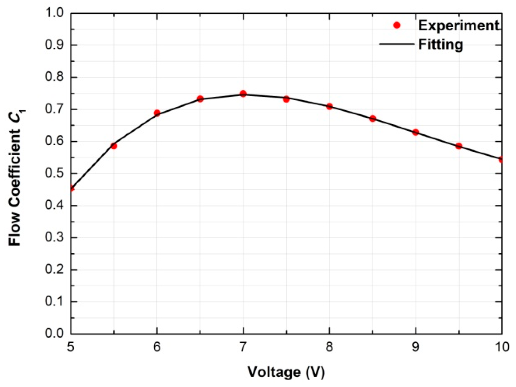
The supply pressure $p_{\mathrm{s}}$ was set at 0.6 MPa, and the values of $p_{\mathrm{s}}$, $T_{\mathrm{s}}$, $\stackrel{.}{M_5}$ and $\stackrel{.}{M_4}$ were measured when the drive voltages of the proportional valve were 5 V, 5.5 V, 6 V, 6.5 V… and 10 V. We took $C_0$ = 0.43; then, the calculation results of the flow coefficient $C_1$ under different driving voltages were obtained from the measured data and Equation (38), as shown in Figure 11. The result reveals that the flow coefficient $C_1$ shows the non-linear variation of a convex function with the increase of the driving voltage.

The driving voltage $U$ of the proportional valve is 0–10 V. When $0\le U<5\mathrm{V}$, the spool moves to the left, and $x_{\mathrm{V}}<0$. When $5\mathrm{V}\le U\le 10\mathrm{V}$, the spool moves to the right, and $x_{\mathrm{V}}>0$. Equation (39) is the relationship between $U$ and $x_{\mathrm{V}}$. Because of the symmetry of the proportional valve, the fourth power equation for calculating the flow coefficient can be obtained based on the polynomial fitting method.

$$\begin{array}{cc}{x}_{\mathrm{V}}=0.0002\left(U-5\right)& 0\le U\le 10\end{array}.$$

(39)

$$C_1=\{\begin{array}{ll}-3.5227\times {10}^{11}{x}_{\mathrm{V}}{}^4+1.8641\times {10}^9{x}_{\mathrm{V}}{}^3-3.133\times {10}^6{x}_{\mathrm{V}}{}^2+1713.94x_{\mathrm{V}}+0.4517& x_{\mathrm{V}}<0\\ -3.5227\times {10}^{11}{x}_{\mathrm{V}}{}^4-1.8641\times {10}^9{x}_{\mathrm{V}}{}^3-3.133\times {10}^6{x}_{\mathrm{V}}{}^2-1713.94x_{\mathrm{V}}+0.4517& x_{\mathrm{V}}\ge 0\end{array}.$$

(40)

5.2. Heat Transfer Coefficient

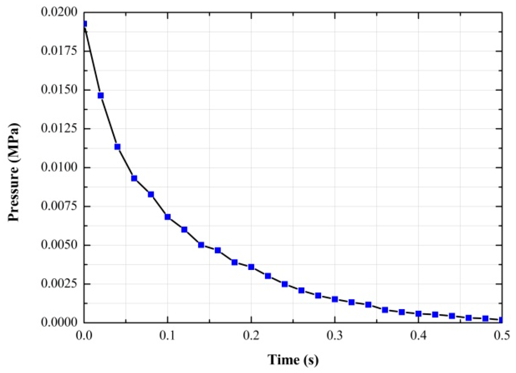
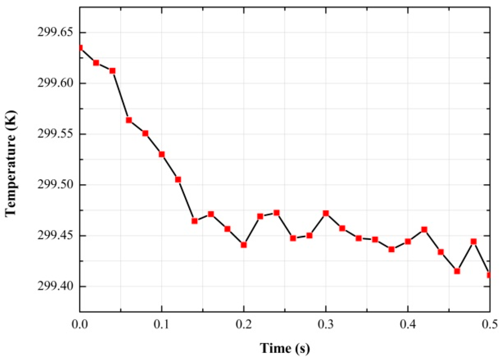
In Figure 12, the piston of chamber a should be fixed at the end during the whole test. First, we charged the chamber a until the chamber reached a steady state. Then, we changed the driving voltage of the proportional valve to discharge the chamber. At this time, the gas pressure $p_{\mathrm{a}}$ and temperature $T_{\mathrm{a}}$ began to decrease. However, the chamber volume $V_{\mathrm{a}}$ was constant. In this process, the pressure differential equation Equation (32) can be simplified as Equation (41), and the energy equation Equation (31) can be simplified as Equation (42). Therefore, we can calculate the heat transfer coefficient $h$ by measuring $T_{\mathrm{a}}$, $\frac{\mathrm{d}{T}_{\mathrm{a}}}{\mathrm{d}t}$, $p_{\mathrm{a}}$ and $\frac{\mathrm{d}{p}_{\mathrm{a}}}{\mathrm{d}t}$ [25].

$$\frac{\mathrm{d}{p}_{\mathrm{a}}}{\mathrm{d}t}=\frac{1}{V_{\mathrm{a}}}\left(-R{T}_{\mathrm{a}}\stackrel{.}{M_{\mathrm{a}}}+\frac{p_{\mathrm{a}}{V}_{\mathrm{a}}}{T_{\mathrm{a}}}\frac{\mathrm{d}{T}_{\mathrm{a}}}{\mathrm{d}t}\right),$$

(41)

$$\frac{c_V{p}_{\mathrm{a}}{V}_{\mathrm{a}}}{R{T}_{\mathrm{a}}}\frac{\mathrm{d}{T}_{\mathrm{a}}}{\mathrm{d}t}=-R{T}_{\mathrm{a}}\stackrel{.}{M_{\mathrm{a}}}+h{S}_{\mathrm{ha}}\left(T_{\mathrm{e}}-T_{\mathrm{a}}\right).$$

(42)

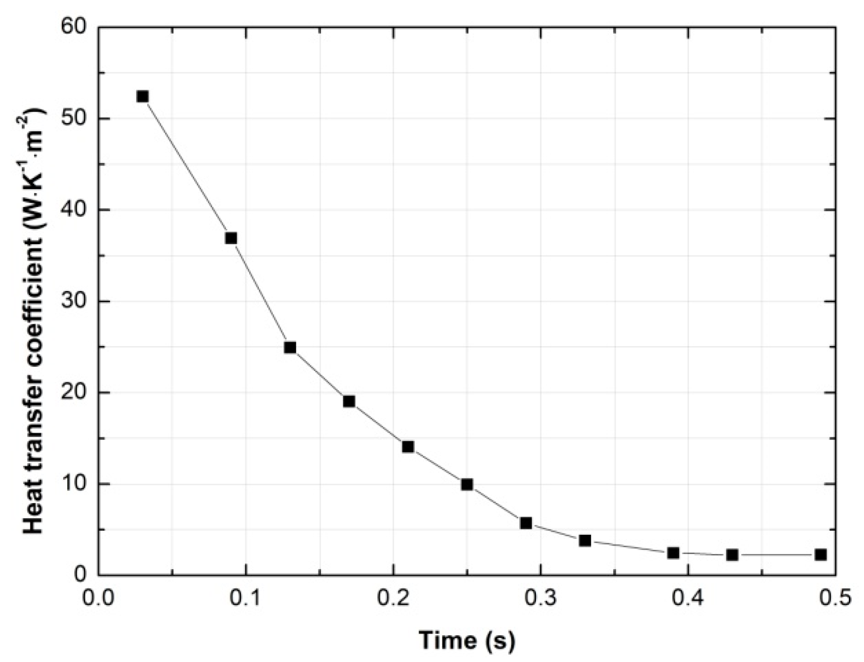
Figure 13, Figure 14 and Figure 15 show the curves of the pressure $p_{\mathrm{a}}$, the temperature $T_{\mathrm{a}}$, and the heat transfer coefficient $h$, respectively. The result shows that the value of heat transfer coefficient is relatively large at first, and then decreases rapidly. Even if the heat transfer coefficient is fixed, high-accuracy solutions of pressure and temperature can be obtained [15]. Therefore, the heat transfer coefficient $h$ in this system can be taken as an average $h$ = 15.797 W/(K·m²).

5.3. Friction Parameters

When the actuator is stationary or moves at a constant speed, ${\mathrm{d}}^2\theta /\mathrm{d}{t}^2=0$. We can obtain Equation (43) by Equation (34), (35) and (37). Therefore, the friction force can be obtained by measuring the pressures in two chambers.

$$F_{\mathrm{f}}=2A\left(p_{\mathrm{a}}-p_{\mathrm{b}}\right).$$

(43)

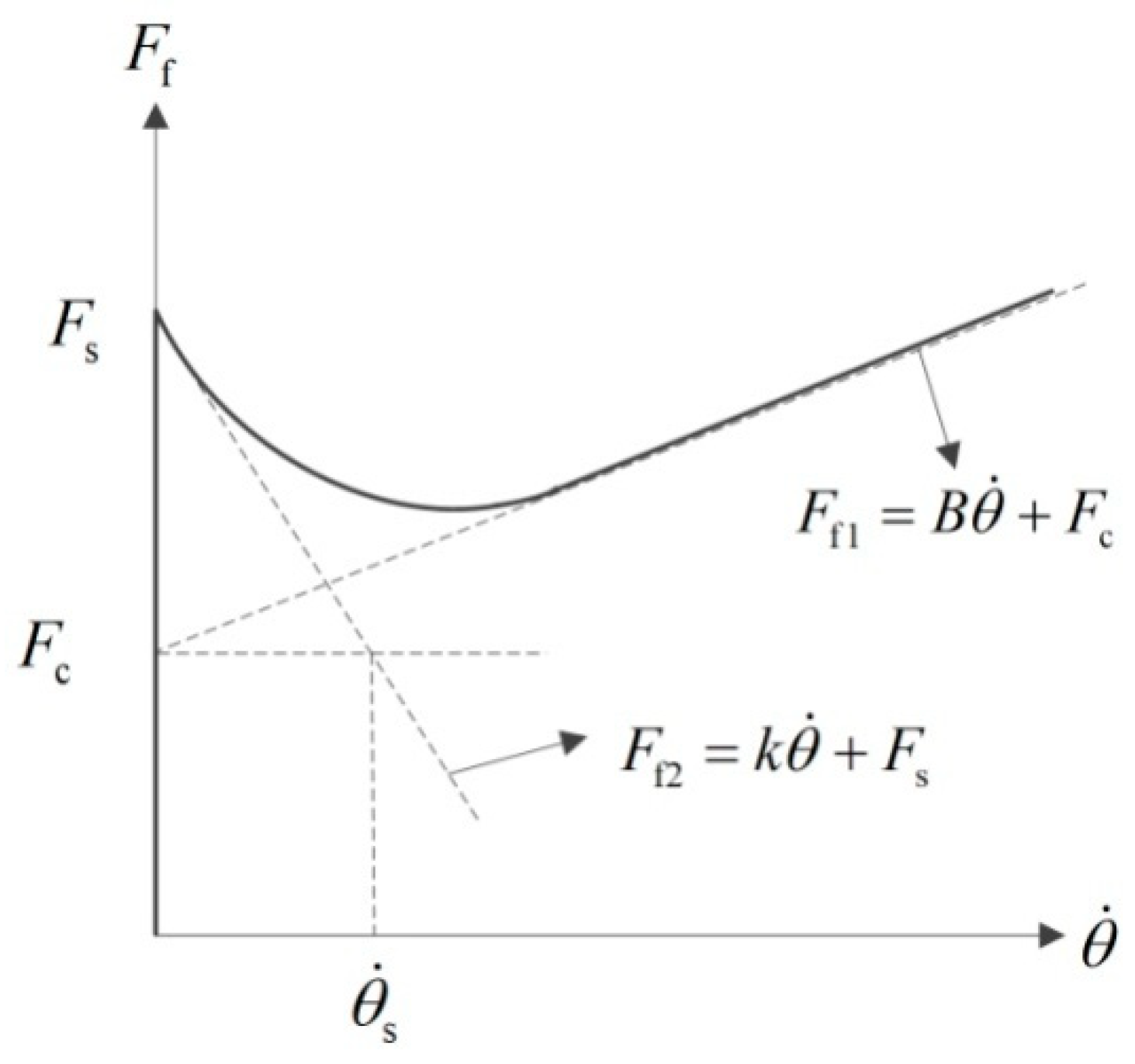
Figure 16 shows the force-speed curve of the Stribeck model. In order to calculate the parameters in the friction model, we assume two straight lines $F_{\mathrm{f}1}=B\dot{\theta }+F_{\mathrm{c}}$ and $F_{\mathrm{f}2}=k\dot{\theta }+F_{\mathrm{s}}$ to obtain the friction parameters by their geometric relations. The curve of the friction force in the high-speed region can be approximated as a straight line $F_{\mathrm{f}1}=B\dot{\theta }+F_{\mathrm{c}}$ whose slope is the value of viscous friction coefficient $B$, and the intersection of this line and the axis of ordinates is Coulomb friction force $F_{\mathrm{c}}$. Moreover, when the piston speed is 0, the maximum value of the friction force is the maximum static friction force $F_{\mathrm{s}}$. The friction curve in the low speed region can be approximated as straight line $F_{\mathrm{f}2}=k\dot{\theta }+F_{\mathrm{s}}$, in which $k$ is the slope. In the line $F_{\mathrm{f}2}=k\dot{\theta }+F_{\mathrm{s}}$, the abscissa ${\dot{\theta }}_{\mathrm{s}}$ corresponding to the ordinate $F_{\mathrm{c}}$ is the Stribeck speed [18].

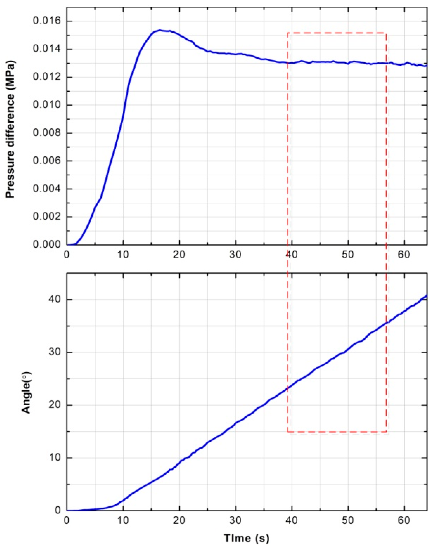
We can identify the friction parameters by using the pneumatic circuit of Figure 1. When the supply pressure $p_{\mathrm{s}}$ was 0.6 MPa and the driving voltage of the proportional valve was 5.07 V, the pressure difference of two chambers and the rotation angle of the actuator were obtained, as shown in Figure 17. In the time interval of the curve labeled by the red column, the actuator moved at a constant speed; then, the friction force value corresponding to this speed can be easily obtained by the pressure difference $\left(p_{\mathrm{a}}-p_{\mathrm{b}}\right)$ and Equation (42).

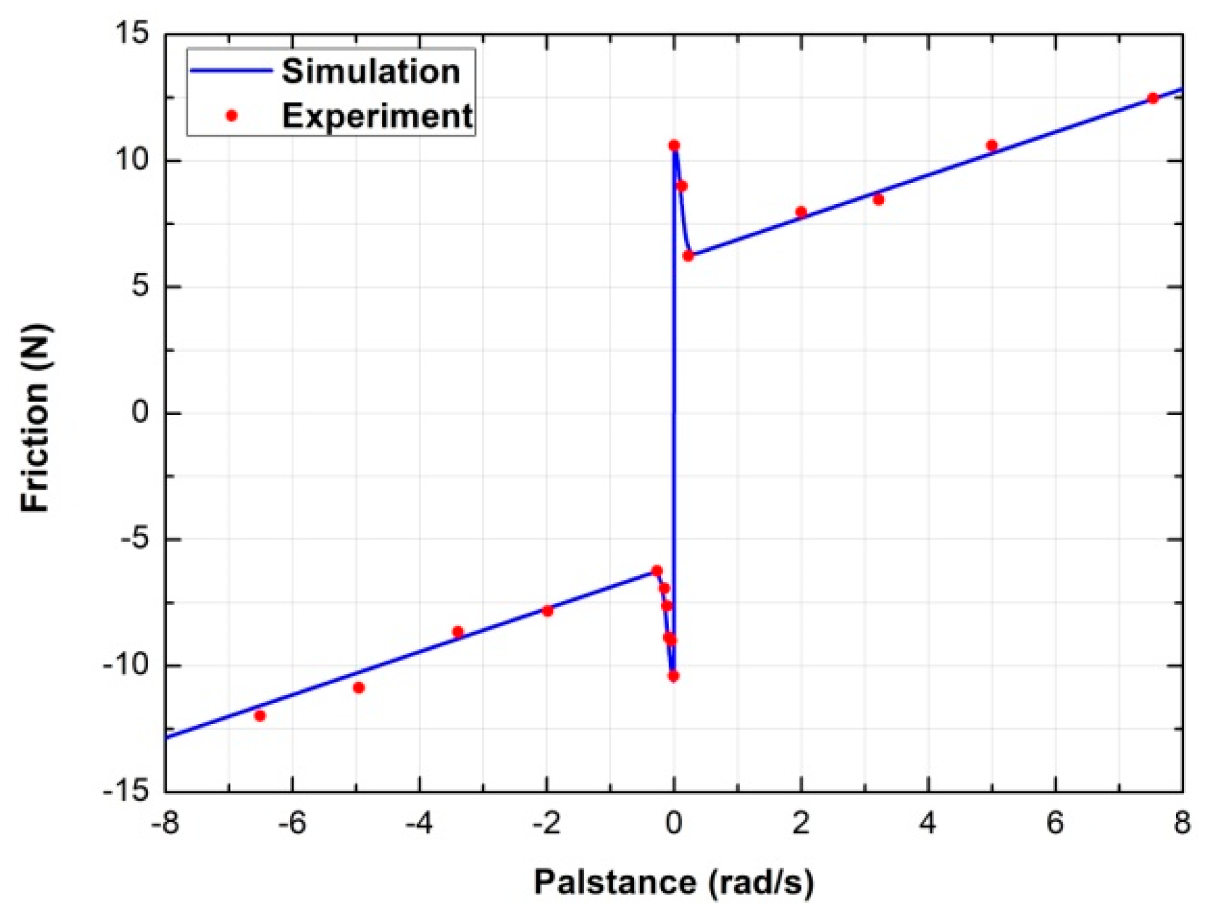
By changing the driving voltage of the proportional valve, we can obtain friction forces at different speeds. The simulation curve and test values of the friction force are compared in Figure 18. The result shows that the test values are consistent with the simulation curve. The friction parameters can be obtained from the geometric relations of Figure 16, as shown in

Table 4. Friction force parameters.

Parameter	Value
$F_{\mathrm{s}}$	10.60 (N)
$F_{\mathrm{c}}$	6.03 (N)
${\dot{\theta }}_{\mathrm{s}}$	0.14 (rad/s)
$B$	0.85 (N·rad−1·s−1)

.

6. Verification of the Non-Linear Model

6.1. Verification of the Mass Flow Rates of the Proportional Valve

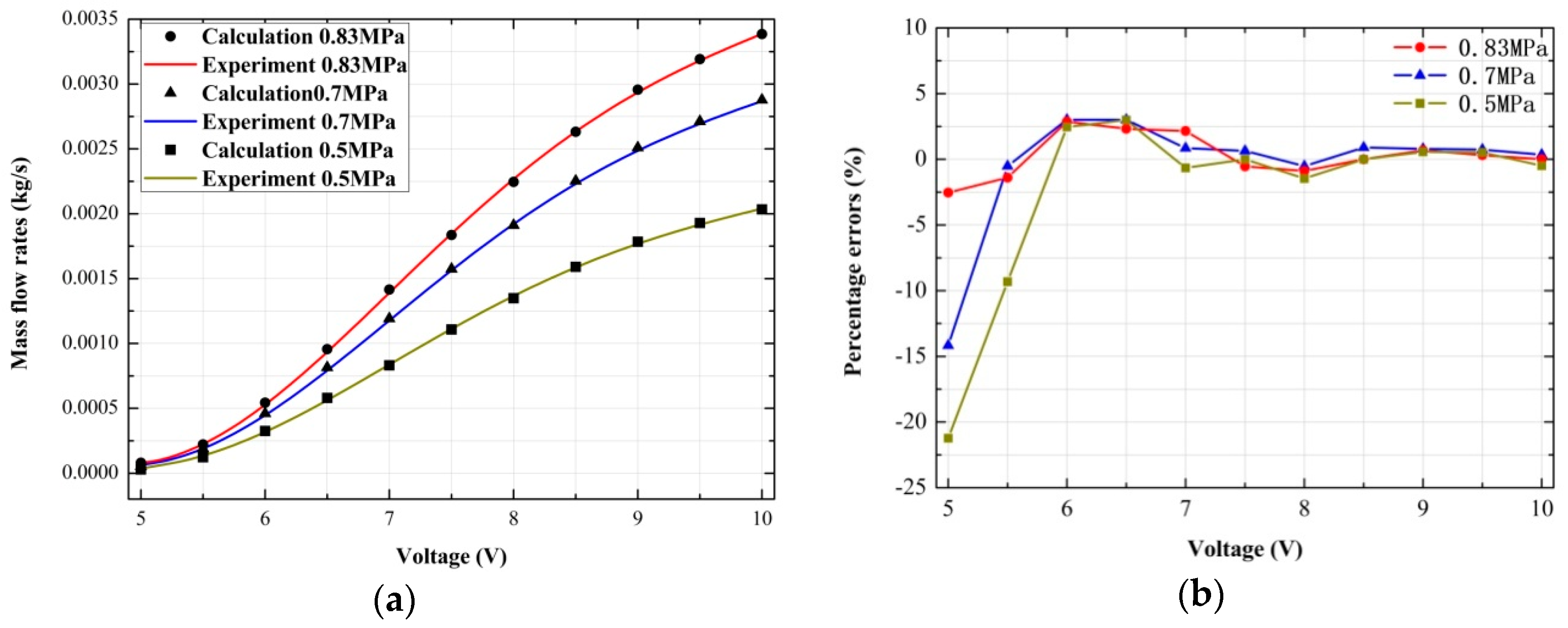
The verification experiment of the mass flow rates was carried out with the pneumatic circuit shown in Figure 10. We set the supply pressure $p_{\mathrm{s}}$ at 0.5 MPa, 0.7 MPa, and 0.83 MPa, and then the mass flow rates $\stackrel{.}{M_4}$ and $\stackrel{.}{M_5}$ under different driving voltages were tested.

The calculation curves of the mass flow rate $\stackrel{.}{M_4}$ were obtained from the calculations of Equations (1), (8) and (17), and were compared with the test values, as shown in Figure 19a. If we take the test values as the actual values, the percentage errors can be expressed by Figure 19b. The result shows that the mass flow rate $\stackrel{.}{M_4}$ increases non-linearly with the driving voltage increasing and that the calculation curves are consistent with the test values. For the whole system, the mass errors are quite small, but when the spool is near the middle position, it shows a relatively large percentage error. This is because an excessively small mass flow rate can magnify the influence of measurement accuracy and calculation error on the results.

In order to fully test the clearance flow of port 5 under different driving voltages and to accurately test the chamber pressure $p_{\mathrm{a}}$ of the proportional valve, we closed ports 2, 3 and 4. Then, the pressure $p_{\mathrm{a}}$ was measured.

Table 5. Chamber pressure $p_{\mathrm{a}}$ of the proportional valve under different driving voltages and supply pressures (MPa).

Driving Voltage	5 V	5.1 V	5.3 V	5.5 V	5.75 V	6 V	6.5 V	7 V	8 V	9 V	10 V
$p_{\mathrm{s}}$ = 0.5 MPa	0.2763	0.3143	0.4046	0.4563	0.475	0.4813	0.4863	0.4863	0.4863	0.4863	0.4863
$p_{\mathrm{s}}$ = 0.7 MPa	0.394	0.4353	0.5583	0.6263	0.6743	0.6713	0.6763	0.6763	0.6763	0.6763	0.6763
$p_{\mathrm{s}}$ = 0.83 MPa	0.4813	0.5263	0.6613	0.7513	0.7863	0.7913	0.7963	0.7963	0.7963	0.7963	0.7963

shows the measured values of the pressure $p_{\mathrm{a}}$.

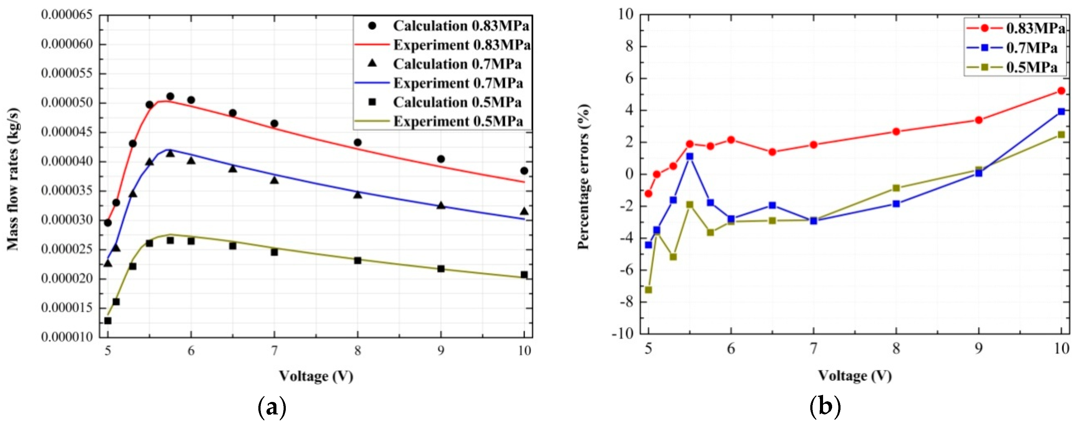
Figure 20 shows the experimental contrast curves of mass flow rate $\stackrel{.}{M_5}$ and their percentage errors. The calculation curves of the mass flow rate $\stackrel{.}{M_5}$ were calculated by Equation (17). The pressure $p_{\mathrm{a}}$ in the calculation was based on the data in Table 5. It can be seen from the Equation (17) that the length of clearance and the pressure of chamber are two factors that affect the clearance flow. Both of these parameters increase with the increase of the driving voltage in this test. Figure 20a shows that the mass flow rates increase first and then decrease. Figure 20b shows their percentage errors. The maximum percentage error is -8.55%.

Therefore, the mass flow rate equations of the proportional directional control valve are well verified by comparing the calculation values with the test values.

6.2. Charging and Discharging of the Chamber with a Certain Volume

The established non-linear model can be further verified by a charging and discharging experiment. The effect of the proportional valve clearance on the gas pressures and the effect of the heat transfer on the gas temperatures can also be studied.

The charging and discharging experiment was carried out with the pneumatic circuit shown in Figure 21. During the whole process, two pistons of the actuator were stationary at the end. The supply pressure $p_{\mathrm{s}}$ was set at 0.6 MPa. The initial driving voltage of the proportional valve was 5 V. When we changed the driving voltage to 5.5 V, chamber a began to charge, and chamber b began to discharge at the same time. $p_{\mathrm{a}}$, $p_{\mathrm{b}}$, $T_{\mathrm{a}}$ and $T_b$ were obtained by Equations (31) and (32) when $V_{\mathrm{a}}$ and $V_{\mathrm{b}}$ were the two constants. The test values of $p_{\mathrm{a}}$, $p_{\mathrm{b}}$, $T_{\mathrm{a}}$ and $T_b$ were measured by the pneumatic circuit shown in Figure 21.

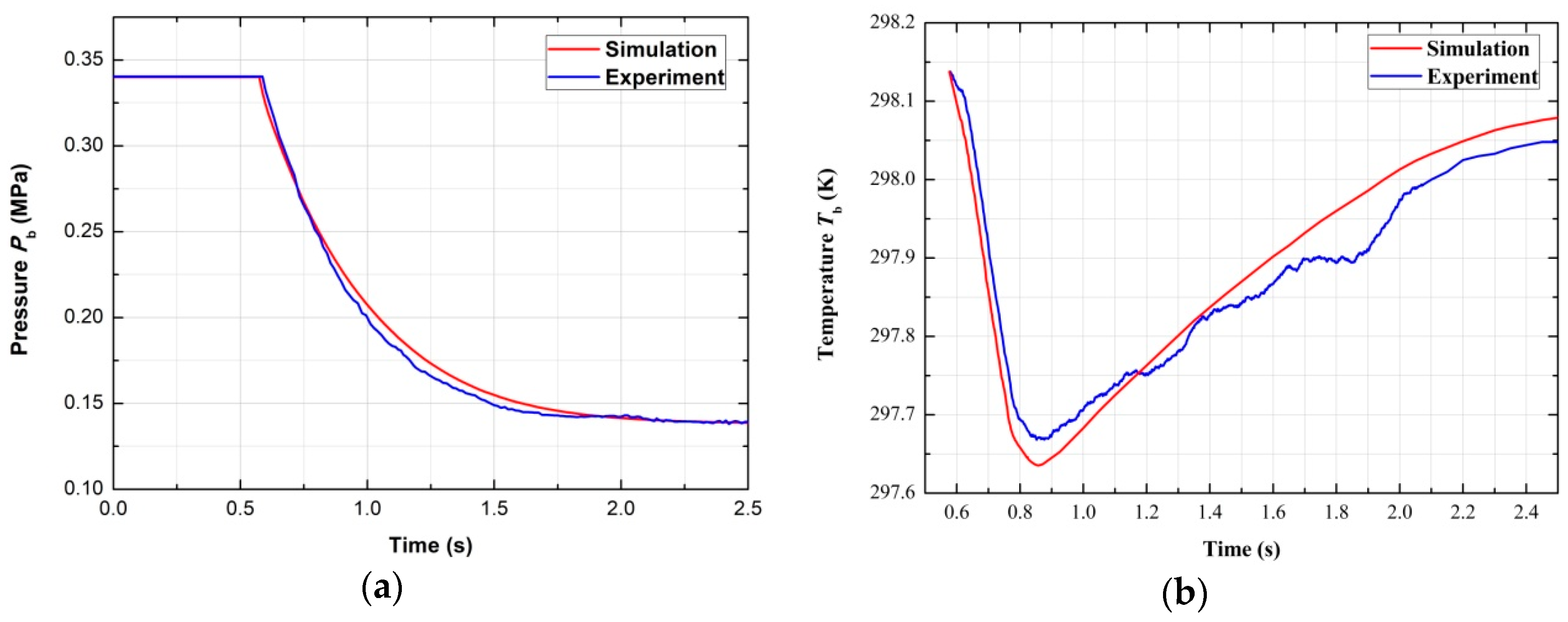
Figure 22 and Figure 23 show the curves of pressure and temperature when chamber a is charging and chamber b is discharging, respectively. The results show that the simulation curves and experimental curves are basically the same.

As shown in Figure 22a, the gas pressure $p_{\mathrm{a}}$ increases from 0.35 MPa to 0.592 MPa gradually and does not reach the value of the supply pressure $p_{\mathrm{s}}$. In Figure 23a, the gas pressure $p_{\mathrm{b}}$ reduces from 0.34 MPa to 0.138 MPa gradually in the discharging process and does not reach the value of atmospheric pressure. With the influence of the clearance, a small amount of gas flows out from chamber a when it is charged, and a small amount of the air supply flows into the chamber b when it is discharged.

The simulation curves of $T_{\mathrm{a}}$ and $T_{\mathrm{b}}$ were verified by comparing their test results, and they are shown in Figure 22b and Figure 23b, respectively. Because of the heat transfer between the gas and the inner wall of the actuator, the gas temperature increases suddenly and then restores to room temperature during the charging process. However, the gas temperature decreases suddenly in a short time and then restores to room temperature during the discharging process.

Therefore, the non-linear model considering the clearance and heat transfer formula can better describe the change of the gas temperatures and pressures in chambers, and it has been well verified.

6.3. Response Verification of the Valve-Controlled Actuator System

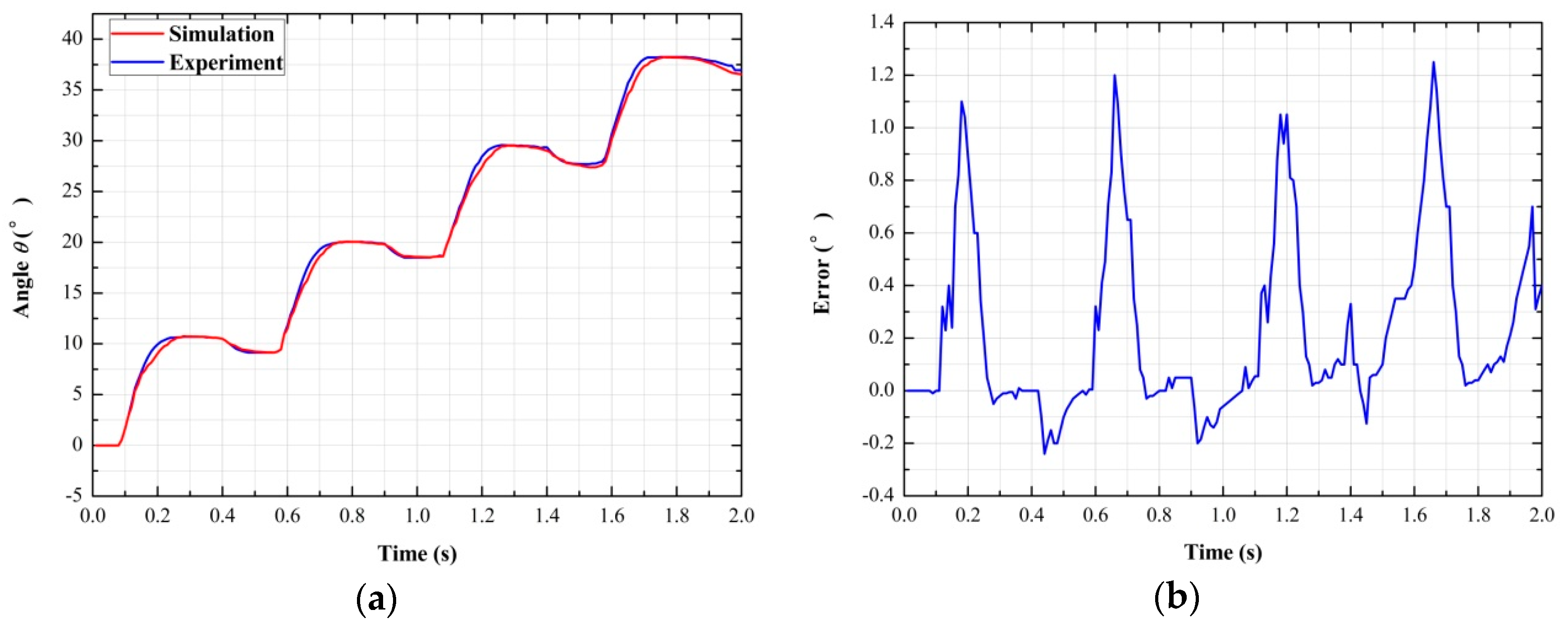
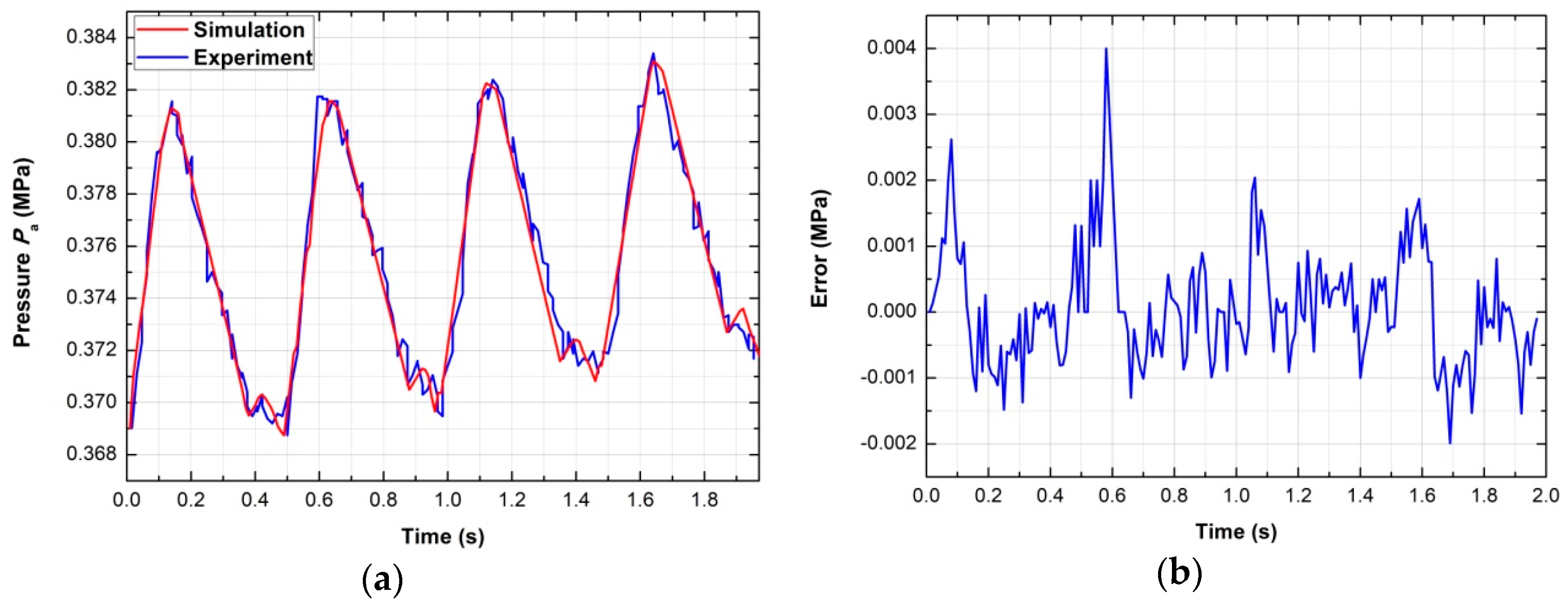
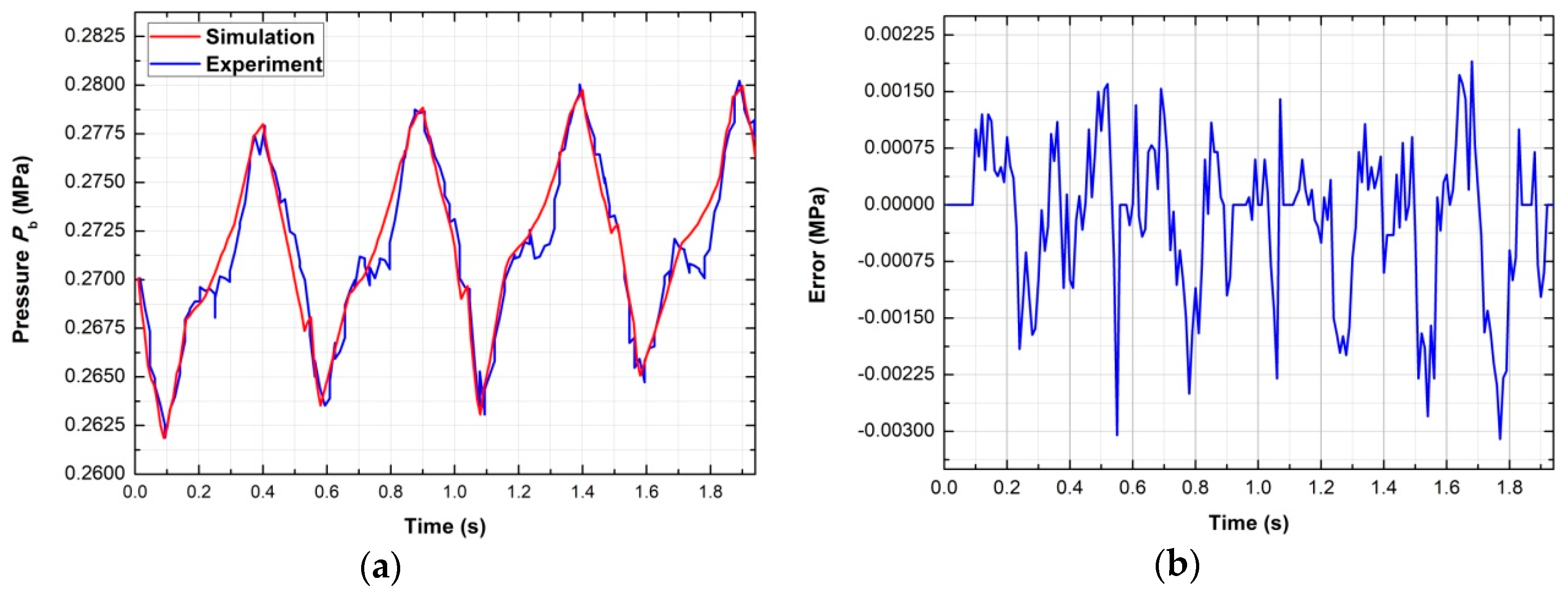
The non-linear model of the valve-controlled actuator system can be verified by the pneumatic circuit shown in Figure 1. The supply pressure $p_{\mathrm{s}}$ was set at 0.6 MPa, and the driving voltage of the proportional valve was the sinusoidal signal with amplitude of 4.65–5.35 V and frequency of 2 Hz. The experimental curves of the rotation angle and the gas pressures are compared with their simulation curves. Figure 24 shows the rotation angle curve and error curve. The maximum error of the angle is not more than 1.25°. Figure 25 shows the pressure curve and error curve of chamber a, whose maximum error is 4 × 10⁻³ MPa. Figure 26 shows the pressure curve and error curve of chamber b, whose maximum error is 3.05 × 10⁻³ MPa.

One part of the experimental errors is the dynamic error generated by the signal acquisition. According to the parameters in Table 1, the accuracies of the rotary encoder and pressure transmitter are 4.5 × 10⁻³ and 0.6 × 10⁻³ MPa, respectively. The measurement errors of instruments are much smaller than the result errors, thus the experiment can still reveal the correct verification results. The experimental curves shown in Figure 24, Figure 25 and Figure 26 are consistent with the trends of the simulation curves, and the errors are within a small range. Therefore, the correctness of the non-linear model has been well verified.

7. Conclusions

In this paper, the mass flow rate equations of the proportional directional control valve were derived from throttled flow and clearance flow by taking into account the clearance between the valve spool and the sleeve. In the modeling of the valve-controlled actuator system, the heat transfer formula was used to the derivation of the energy equation, and the Stribeck model was applied to the friction model of the pneumatic rotary actuator. The flow coefficient of the proportional valve was tested by the pneumatic test circuit. The heat transfer coefficient and friction parameters were also obtained from the model and pneumatic test circuits. The mass flow rate equations were verified by the experiment and showed great precision. The charging and discharging experiment reveals that the clearances affect two chamber pressures, and that the heat transfer between the gas and the actuator inner wall also affects the gas temperatures. Finally, the non-linear model was verified by the experiment. The results show that the simulation curves of the rotation angle and two chamber pressures are consistent with the experimental curves. The errors of the rotation angle are within 1.25°, while the errors of the pressures do not exceed 4×10⁻³ MPa. The established non-linear model can accurately reflect the characteristics and the motion states of the pneumatic rotary actuator position servo system. The results of the study are important for the theory and practice of pneumatic servo systems.

References

- Shi, Y.; Wu, T.; Cai, M.; Wang, Y.; Xu, W. Energy conversion characteristics of a hydropneumatic transformer in a sustainable-energy vehicle. Appl. Energy 2016, 171, 77–85. [Google Scholar] [CrossRef]
- Jia, G.; Xu, W.; Cai, M.; Shi, Y. Micron-sized water spray-cooled quasi-isothermal compression for compressed air energy storage. Exp. Therm. Fluid Sci. 2018, 96, 470–481. [Google Scholar]
- Zhang, Y.M.; Cai, M.L. Overall life cycle comprehensive assessment of pneumatic and electric actuator. Chin. J. Mech. Eng. 2014, 27, 584–594. [Google Scholar] [CrossRef]
- Shaw, D.; Yu, J.-J.; Chieh, C. Design of a hydraulic motor system driven by compressed air. Energies 2013, 6, 3149–3166. [Google Scholar] [CrossRef]
- Ning, F.; Shi, Y.; Cai, M.; Wang, Y.; Xu, W. Research progress of related technologies of electric-pneumatic pressure proportional valves. Appl. Sci. 2017, 7, 1074. [Google Scholar] [CrossRef]
- Saravanakumar, D.; Mohan, B.; Muthuramalingam, T. A review on recent research trends in servo pneumatic positioning systems. Precis. Eng. 2017, 49, 481–492. [Google Scholar] [CrossRef]
- Shearer, J.L. Study of pneumatic processes in the continuous control of motion with compressed air-I. Trans. ASME 1956, 233–242. [Google Scholar]
- Zhang, Y.; Li, K.; Wei, S.; Wang, G. Pneumatic Rotary Actuator Position Servo System Based on ADE-PD Control. Appl. Sci. 2018, 8, 406. [Google Scholar] [CrossRef]
- Li, K.; Zhang, Y.; Wei, S.; Yue, H. Evolutionary Algorithm-Based Friction Feedforward Compensation for a Pneumatic Rotary Actuator Servo System. Appl. Sci. 2018, 8, 1623. [Google Scholar] [CrossRef]
- Rao, Z.; Bone, G.M. Nonlinear modeling and control of servo pneumatic actuators. IEEE Trans. Control Syst. Technol. 2008, 16, 562–569. [Google Scholar]
- Lee, L.-W.; Li, I.-H. Wavelet-based adaptive sliding-mode control with h∞ tracking performance for pneumatic servo system position tracking control. IET Control Theory A. 2012, 6, 1699–1714. [Google Scholar] [CrossRef]
- Harris, P.G.; O’Donnell, G.E.; Whelan, T. Modelling and identification of industrial pneumatic drive system. Int. J. Adv. Manuf. Technol. 2012, 58, 1075–1086. [Google Scholar] [CrossRef]
- Van der Merwe, J.; Muller, J.; Scheffer, C. Parameter identification and evaluation of a proportional directional flow control valve model. R&D J. South Afr. Inst. Mech. Eng. 2013, 29, 18–25. [Google Scholar]
- Rad, C.-R.; Hancu, O. An improved nonlinear modelling and identification methodology of a servo-pneumatic actuating system with complex internal design for high-accuracy motion control applications. Simul. Model. Pract. Theory 2017, 75, 29–47. [Google Scholar] [CrossRef]
- Cai, M. Second: Fixed volume cavity charging and discharging. Hydraul. Pneum. Seals 2007, 27, 43–47. (In Chinese) [Google Scholar]
- Valdiero, A.C.; Ritter, C.S.; Rios, C.F.; Rafikov, M. Nonlinear mathematical modeling in pneumatic servo position applications. Math. Probl. Eng. 2011, 2011, 472903. [Google Scholar] [CrossRef]
- Bai, Y.-H.; Li, X.-N. Dual-loop Control Strategy with Friction Compensation for Pneumatic Rotary Actuator Position Servo System. J.-Nanjing Univ. Sci. Technol. 2006, 30, 216. [Google Scholar]
- Xu, J.; Qiao, M.; Wang, W.; Miao, Y. Fuzzy PID control for AC servo system based on Stribeck friction model. In Proceedings of the 2011 6th International Forum on Strategic Technology, Harbin, China, 22–24 August 2011; IEEE: Harbin, China, 2011; Volume 2, pp. 706–711. [Google Scholar]
- Kong, X.; Wang, Y.; Jiang, S. Friction Chatter-compensation Based on Stribeck Model. J. Mech. Eng. 2010, 46, 68–73. [Google Scholar] [CrossRef]
- Zhang, S.; Chen, J.B.; Wang, T.; Fan, W. Nonlinear modeling and simulation of pneumatic servo position system of rodless cylinder. In Applied Mechanics and Materials; Trans Tech Publications: Zürich, Switzerland, 2012; Volume 130, pp. 3493–3497. [Google Scholar]
- Peter, B. Pneumatic Drives System Design, Modeling and Control; Springer: Berlin/Heidelberg, Germany, 2007. [Google Scholar]
- Sanville, F. A new method of specifying the flow capacity of pneumatic fluid power valves. Hydraul. Pneum. Power 1971, 17, 120–126. [Google Scholar]
- Daugherty, R.L.; Ingersoll, A.C. Fluid Mechanics; McGraw-Hill Book Company, Inc.: New York, NY, USA, 1954. [Google Scholar]
- Zhan, Y.J.; Wang, T.; Wang, B. Study on friction characteristics of energizing pneumatic cylinders. In Advanced Materials Research; Trans Tech Publications: Zürich, Switzerland, 2014; Volume 904, pp. 306–310. [Google Scholar]
- Carneiro, J.; de Almeida, F.G. Heat transfer evaluation of industrial pneumatic cylinders. Proc. Inst. Mech. Eng. Part 1 2007, 221, 119–128. [Google Scholar] [CrossRef] [Green Version]
Figure 1.
Schematic diagram of the pneumatic rotary actuator position servo system (1—air compressor; 2—air filter; 3—air regulator; 4—air lubricator; 5—pressure transmitter; 6—proportional directional control valve; 7—rotary encoder; 8—pneumatic rotary actuator; 9—IPC).
Figure 2.
Experimental platform of the pneumatic rotary actuator position servo system.
Figure 3.
Schematic diagram of the valve-controlled actuator system.
Figure 4.
Gas flow mechanism when the spool moves toward the positive direction.
Figure 5.
Flow splitting through orifice.
Figure 6.
Relative position of the circular hole and the spool shoulder: (a) Initial position; (b) Relative position when displacement is .
Figure 7.
Physical area of the orifice in the horizontal direction.
Figure 8.
Schematic diagram of the clearance flow.
Figure 9.
Gas flow mechanism when the spool moves backward.
Figure 10.
Pneumatic circuit for testing the flow coefficient : (a) Schematic diagram; (b) Test platform.
Figure 11.
Curve of the flow coefficient under different driving voltages.
Figure 12.
Pneumatic circuit for testing the heat transfer coefficient : (a) Schematic diagram; (b) Test platform.
Figure 13.
Curve of the pressure .
Figure 14.
Curve of the temperature .
Figure 15.
Curve of the heat transfer coefficient .
Figure 16.
Force-speed curve of the Stribeck model.
Figure 17.
Dynamic process of the actuator at low speed.
Figure 18.
Curve of the friction force.
Figure 19.
Curves of mass flow rate with different driving voltages and their errors: (a) Mass flow rates; (b) Percentage errors between calculated and simulated values.
Figure 20.
Figure 21.
Pneumatic circuit for charging and discharging: (a) Schematic diagram; (b) Test platform.
Figure 22.
Curves of pressure and temperature when chamber a is charging: (a) Pressure curves; (b) Temperature curves.
Figure 23.
Curves of pressure and temperature when chamber b is discharging: (a) Pressure curves; (b) Temperature curves.
Figure 24.
Rotation angle curve and its error curve: (a) Rotation angle curve; (b) Error.
Figure 25.
Pressure curve of chamber a and its error curve: (a) Pressure curve; (b) Error.
Figure 26.
Pressure curve of chamber b and its error curve: (a) Pressure curve; (b) Error.