An Adaptive Particle Swarm Optimization Algorithm Based on Guiding Strategy and Its Application in Reactive Power Optimization

Abstract

An improved adaptive particle swarm algorithm with guiding strategy (GSAPSO) was proposed, and it was applied to solve the reactive power optimization (RPO). Four kinds of particles containing the main particles, double central particles, cooperative particles and chaos particles were introduced into the population of the developed algorithm, which was to decrease the randomness and promote search efficiency through guiding particle position updating. Moreover, the cluster focus distance-changing rate was responsible for dynamically adjusting inertia weight. Then the convergence rate and accuracy of this algorithm would be elevated by four functions, which would test effectively the proposed. Finally, the optimized algorithm was verified on the RPO of the IEEE 30-bus power system. The performance of PSO, Random weight particle swarm optimization (WPSO) and Linearly decreasing weight of the particle swarm optimization algorithm (LDWPSO) were identified as the referential information, the proposed GSAPSO was more efficient from the comparison. Calculation results demonstrated that higher quality solutions were obtained and convergence rate and accuracy was significantly higher with regard to the GSAPSO algorithm.

1. Introduction

Reactive power optimization (RPO) has become more and more crucial as a segment of optimal power flow calculation, with the rapid development of China’s power grid and the continuous expansion of its scale. The RPO is equal to reasonably distributing reactive power generation for minimizing the active power losses and maintaining all bus voltages within a reasonable range, while satisfying some constraints [1,2,3,4]. The way to achieve the aforementioned aims depends on the capacity of shunt capacitors, the output of generators and the adjustment of transformer tap positions [5,6,7,8].

Generally, the nonlinear characteristic is prominent in RPO and is composed of multivariate, multi-constraint, discrete variables and continuous variables. A number of conventional optimization methods or techniques, traditional linear programming (LP) [9], Newton method [10], quadratic programming (QP) [11], and interior point method (IPM) [12], were put forward to deal with RPO. However, due to discontinuity and multi-peak, these techniques did not handle well. In recent years, some of the heuristic algorithms such as genetic algorithm (GA) [8,13], simulated annealing (SA) [14], differential evolution (DE) [15,16], improved shuffled frog leaping algorithm (ISFLA) [17], gray wolf optimizer (GWO) [18], particle swarm optimization (PSO) [19,20,21,22] have been widely developed for solving RPO, and have achieved good results. As a clustering intelligence algorithm, the PSO algorithm simulates the behaviour of bird flock foraging, and achieves the goal of optimization through the cooperation and competition among flock birds [23]. Compared to other heuristic techniques, the PSO has a few adjustment parameters and a simple implementation. However, with the increase of variables and more local optimum in the objective function, the PSO algorithm is susceptible to prematurely converging and being put into local optimum. Many researchers have proposed and published potential improvements to the PSO algorithm, which can improve the global and local search ability and avoid the above phenomenon. Kannan et al. [24] proposed a solution for the capacitor optimization configuration in radial distribution using Multi-Agent Particle Swarm Optimization. Zad et al. [25] considered the reactive power control of distributed generations by implementing PSO. Achayuthakan et al. [26] proposed a PSO for RPO achieving reactive power cost allocation. Esmin et al. [22] presented a method to lessen power loss via a hybrid PSO with a mutation operator. Differentially perturbed velocity was used to improve PSO for the ORPD problem of a power system in [27]. Singh et al. [19] presented a new PSO for the scheme of optimal reactive power dispatch (ORPD), where improvement was the introduction of an aging leader and challengers.

In this paper, an improved PSO based on a guiding strategy ws developed, which optimized the particle update mode and the adjustment mechanism of inertia weight, which had no negligible impact on the PSO algorithm. In addition, it was applied in order to solve the PRO in a power system and the standard IEEE 30-bus power system was employed. The effectiveness of the GSAPSO was contrasted to classical PSO, random weight PSO (WPSO) and linearly decreasing weight PSO (LDWPSO).

The structure of this paper is presented as follows: A brief description of PSO is brought out in Section 2. Section 3 presents details of improved PSO. Section 4 provides referential methods to test the three PSO algorithms and the comparison is discussed. Section 5 introduces the formulation of the RPO problem, and the solution algorithms are outlined in Section 6. Section 7 exhibits the simulation results showing the solution effectiveness. Conclusions are given in Section 8.

2. Original Particle Swarm Optimization (PSO)

PSO defines the variables in the solution space as particles without weight and volume. Each particle has two important elements: Velocity and position. The velocity makes a dynamic adjustment on the basis of the flight experience of individuals and groups. The position refers to a potential solution, and the corresponding fitness value can be obtained to judge the quality of the position. Each particle determines the velocity and direction of the flight according to its current location, the optimal location of the individual and the group.

In the S-dimensional space, a randomly initialized population with m particles is generated. The information for each particle i contains its position (X_i = [x_i1, x_i2, …, x_is]) and velocity (V_i = [v_i1, v_i2, …, v_is]), the best value of position for particle i is referred to as P_i = [p_i1, p_i2, …, p_is], whose fitness value is expressed as ‘pbest’. Moreover, the best value of the position for the group is recorded as P_g = [p_g1, p_g2, …, p_gs], and its fitness value is expressed as ‘gbest’. In the searching procedure, the velocity and position of each particle are constantly updated through Equations (1) and (2) respectively.

$$V_{id}^{k+1}={\omega }^k{V}_{id}^k+c_1{r}_1(P_{id}^k-X_{id}^k)+c_2{r}_2(P_{gd}^k-X_{id}^k)$$

(1)

$$X_{id}^{k+1}=X_{id}^k+V_{id}^{k+1}$$

(2)

where k is time of current iteration; r₁ and r₂ are random variables taken between 0 and 1; ω^k is the inertia weight at the kth iteration. c₁ and c₂ are acceleration coefficients. P_id^k is the best value of the ith particle in d dimension. P_gd^k is the best value among the entire population. The velocity range of the particles should be set in case the particle flies out of the search space too quickly and improve optimization ability simultaneously.

3. Adaptive Particle Swarm Algorithm with Guiding Strategy(GSAPSO)

In order to prevent blind search during the early stage and slow search speed as well as easily trap in the local optimum in the later period, the GSAPSO was proposed. The GSAPSO was mainly improved in two aspects, one was the mixed particles update mode, on the other hand, the inertia weight was improved.

3.1. Strategy for Mixed Particles Update

The standard PSO algorithm initializes the population randomly and has strong randomness. To get better performance in convergence, the particles were divided into four parts in this paper. The first part was the main particles randomly generated in system. The second part consisted of two kinds of central particles [28], which were the central particles produced by the first part and the central particles formed by the individual optimal value of all the particles, respectively.

Usually, the optimal solution has a higher probability of appearing in the center position. Therefore, the central particles are used to accelerate the convergence. In the whole search process, the properties of them were the same as those of ordinary particles, except that they had no velocity characteristics.

In the searching process, the two particles with the worst fitness value in the main particles were replaced by the double central particles, and then the particles were prone to fly towards better searching areas.

The third part was cooperative particles. The idea was to make multiple independent particles start from the global optimal position, first updated in one dimension, and then extra particles were updated randomly in the D dimension. The cooperative particles were used to enhance the capability in global search. The fourth part introduced chaotic particles, generated by logistic mapping. The chaotic particles were used to search for sub-optimal solutions of particles in the region around the boundary. The idea of updating the mixed particles was to exchange the good values obtained by the second, third, and fourth parts with the poor values of the first part during each iteration, so that the whole particles approached the best solution.

(1)

The central particles were expressed as Equations (3) and (4).

$$x_{SCP}=1/n{\displaystyle \sum _{i=1}^n{x}_{id}}$$

(3)

$$x_{GCP}=1/n{\displaystyle \sum _{i=1}^n{P}_{id}}$$

(4)

where n represents the quantity of main particles; x_SCP and x_GCP are the central particle produced by the main particles and the individual optimal values, respectively.

(2)

The cooperative particles update formula was as follows

$$x_{id}=P_{gd}+rand\times vec$$

(5)

$$vec=V_{i\max }\times (1-\alpha \times \frac{exetime}{gen})$$

(6)

where vec is a velocity variable whose value can be obtained according to Equation (6). The exetime, gen represents the current number and the total number of iterations respectively. α is the update coefficient. The rand is a random variable taken between 0 and 1 and obeys uniform distribution.

(3)

The chaotic particles were determined as follows

$$\{\begin{array}{l}k=4\times k\times (1-k)\\ x_{id}=x_{i\min }+k\times (x_{i\max }-x_{i\min })\end{array}$$

(7)

where x_imax, x_imin are the maximum and minimum of the coordinates. k is the chaotic factor.

The update of the first part of the main particles was obtained by Equations (1) and (2); the update of the second part of central particles could be obtained by the Equations (3) and (4); and the third part of cooperative particles update formula was shown by Equations (5) and (6). The fourth part of chaotic particles could be updated by Equation (7).

3.2. Strategy for Inertia Weight

ω^k controls the influence of speed in the kth iteration on the speed in the k + 1th iteration, and ω of the standard PSO algorithm can be regarded as 1.0. The larger the inertia term value, the stronger the global search ability. Conversely, the smaller the inertia term value, the stronger the local search ability. Therefore, the size of ω could be dynamically adjusted according to different periods during the iterative process to balance the ability of local and global explorations. In [29], the LDWPSO was proposed, which linearly reduced the ω value during the iterative process. The principle of the LDWPSO algorithm was that ω was larger for the global search in the initial iteration, while the ω value in the later iteration was smaller, and it was easily put into the local optimum. In [30], a dynamic adaptive nonlinear inertia weight was introduced into the PSO. The algorithm judged the particle distribution of the population by the size of the focus distance-changing rate, and then updated dynamically the nonlinear inertia weight according to different situations, which updated the fitness of particles at a suitable speed, and had the capability of good global search ensuring the convergence speed.

The adjustment strategy of inertia weight was to find the Euclidean spatial distance between all particles and the historical optimal in the population. The distance represented the closeness of the particles to the optimal position. The formulas of the average and maximum focus distance are described as follows:

$$Dis{t}_{mean}=\frac{{\displaystyle \sum _{i=1}^m\sqrt{{\displaystyle \sum _{d=1}^D{(X_{id}-P_{gd})}^2}}}}{m}$$

(8)

$$Dis{t}_{\max }=\underset{i=1,2,\dots n}{\max }(\sqrt{{\displaystyle \sum _{d=1}^D{(X_{id}-P_{gd})}^2}})$$

(9)

where m is the quantity of particles in the population. D is the quantity of dimensions of each particle. P_gd is the best position of the population. X_id is the best position of the individual.

Then we could get the current focus distance-changing rate of the particle:

$$k=\frac{Dis{t}_{\max }-Dis{t}_{mean}}{Dis{t}_{\max }}$$

(10)

In the iterative process, the inertia weight was adjusted by the focus distance changing rate, thereby adjusting the ability of the global and the local search. The inertia weight update in [30] was not ideal. After continuous experiment, it was found that the convergence of the algorithm was excellent when the variation curve of the inertia weight with k showed a downward convex trend. Therefore, the Formula (11) was adapted to calculate $\omega$.

$$\omega =\{\begin{array}{ll}\ln (a-k)+b& k\ge 0.05\\ 0.75+rand/4& k<0.05\end{array}$$

(11)

where the rand was a random variable taken between 0 and 1 and obeyed uniform distribution. Compared with the linear decreasing weight method, this selection strategy could better adapt to the complex actual environment, adjust the ability of global and local search more flexibly, and the diversity of the population could be preserved simultaneously.

4. Experiment

4.1. Experimental Setup

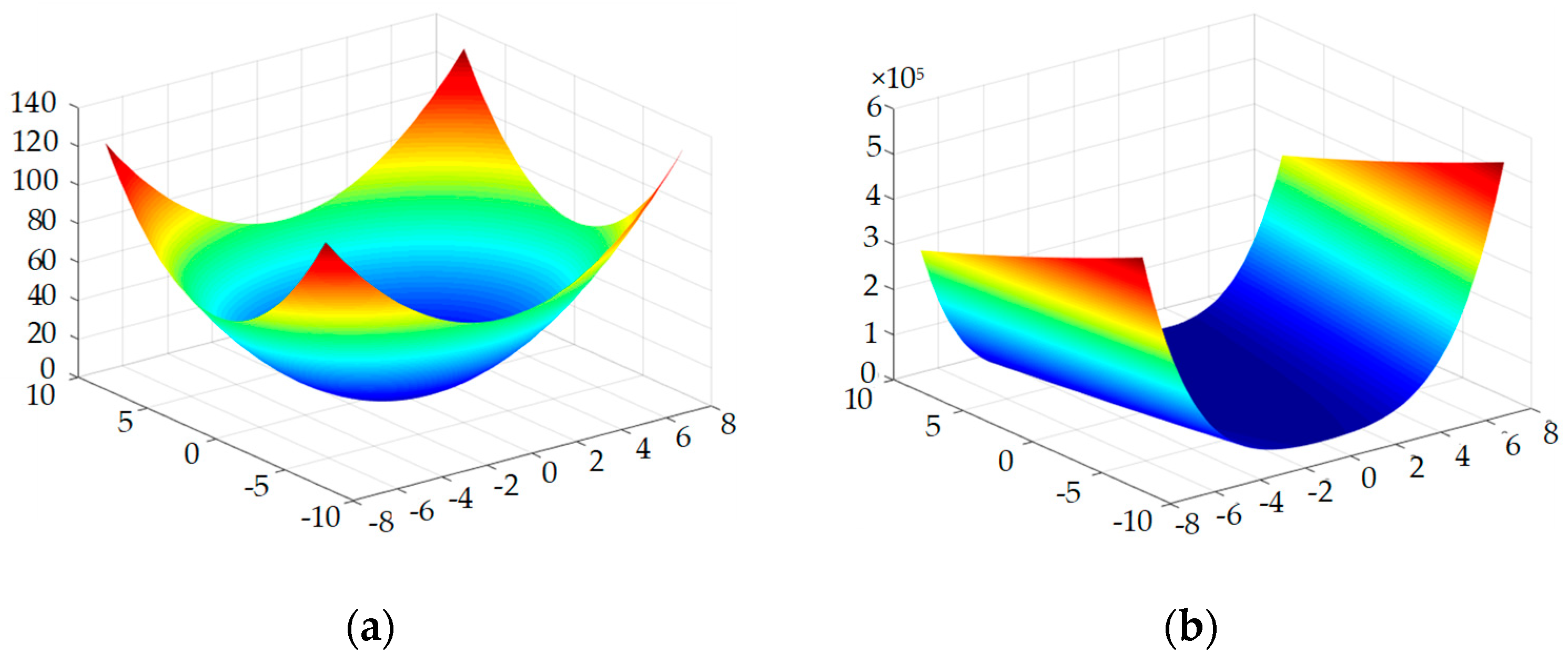
In this section, the comparison of optimized algorithm and WPSO and LDWPSO was carried out by means of classical Benchmark functions consisting of the Sphere function, Rosenbrock function, Rastrigin function and Griewank function, which the performance test generally used. The details of four functions are presented as Figure 1:

(1)

Sphere Function

    The Sphere function is nonlinear and symmetric, it has a single-peak, which can be separated with different dimensions. It is used to test the optimization precision.

(2)

Rosenbrock Function

  The Rosenbrock function is a typical ill-conditioned function that is difficult to minimize. Since this function provides little information for the search, it is difficult to identify the search direction, and the chance of finding the global optimal solution is low. Therefore, it is often used to evaluate the execution performance.

(3)

Rastrigin Function

    The Rastrigin function is a complex multi-peaks function, with large quantity of local optima. It is prone to making the algorithm put local optimum, which will prematurely converge and not get the global optimal solution.

(4)

Griewank Function

    The Griewank function is also a complex multi-peaks function with a large quantity of local minimum.

4.2. Parameter Settings

For the four functions, the optimal objective values were all zero. The maximum number of iterations in the first and fourth functions was set to 1000, and that was 2000 in the second and third functions. The population size was 60, the main particle accounted for 70%, including two central particles, the cooperative particles accounted for 20%, and the chaotic particles accounted for 10%. Learning factor c₁ = c₂ = 2, inertia weight in LDWPSO algorithm was ω_max = 0.9, ω_min = 0.3. Each function used each algorithm to run 10 times independently.

Table 1. Related information of four functions.

Function	Function Expression	Dimension	Range
Sphere	$f_1={\displaystyle \sum _{i=1}^n{x}_i^2}$	30	${\left[-100,100\right]}^n$
Rosenbrock	$f_2={\displaystyle \sum _{i=1}^{n-1}\left[100{(x_{i+1}-x_i^2)}^2+{(x_i-1)}^2\right]}$	10	${\left[-30,30\right]}^n$
Rastrigin	$f_3={\displaystyle \sum _{i=1}^n\left[x_i^2-10\cos (2\pi x_i)+10\right]}$	10	${\left[-5.12,5.12\right]}^n$
Griewank	$f_4=\frac{1}{4000}{\displaystyle \sum _{i=1}^n{x}_i^2-{\displaystyle \prod _{i=1}^n\cos (\frac{x_i}{\sqrt{i}})}}+1$	30	${\left[-600,600\right]}^n$

shows the relevant information of four functions.

4.3. Analysis of Test Results

For LDWPSO, WPSO and the GSAPSO algorithms, the convergence accuracy and speed of the algorithms were analyzed respectively. The statistical results of the experiment are shown in

Table 2. Convergence accuracy of GSAPSO, LDWPSO, WPSO algorithms.

Functions	GSAPSO			LDWPSO			WPSO
	BEST	WORST	MEAN	BEST	WORST	MEAN	BEST	WORST	MEAN
Sphere	9.38 × 10−27	2.81 × 10−22	4.86 × 10−23	7.27 × 10−13	1.85 × 10−11	9.53 × 10−12	1.01 × 10−4	1.36 × 10−2	2.73 × 10−3
Rosenbrock	1.25 × 10−4	2.29	1.31	0.0837	5.795	2.975	1.81	10.187	4
Rastrigin	0	0	0	0	2.985	1.393	0	3.98	1.89
Griewank	0	0.0465	9.33 × 10−3	7.7 × 10−13	0.032	0.0133	6.49 × 10−4	0.0623	0.0222

and

Table 3. Convergence speed of GSAPSO, LDWPSO and WPSO algorithms.

Functions	GSAPSO			LDWPSO			WPSO
	AT	BT	SR	AT	BT	SR	AT	BT	SR
Sphere	148	119	100%	644	623	100%	685	571	90%
Rosenbrock	1626	118	20%	2000	1090	-	2000	1944	-
Rastrigin	126	84	100%	1762	1081	20%	1704	513	20%
Griewank	321	125	80%	790	622	60%	871	620	40%

.

(1) Algorithm convergence accuracy analysis

According to the parameter setting in Section 4.2, the convergence precision of the three PSO algorithms was counted in the same conditions. The best value (BEST), the mean value (MEAN), and the worst value (WORST) of the objective function in ten iterations could characterize the performance of each algorithm. From Table 2, it demonstrated that the GSAPSO was superior to the others for the BEST, the MEAN, and the WORST. Moreover, the three types of values of GSAPSO algorithm were not much different, which indicated that the GSAPSO had better stability. The results of the Sphere function reflected the GSAPSO algorithm was much faster than the LDWPSO and WPSO algorithms to obtain the optimal value. The Rosenbrock function was more complex, and the optimization result not only reflected the convergence speed of the algorithm, but reflected the ability of jumping out local optimum. Therefore, it could be seen that the GSAPSO had a higher convergence accuracy than the others. For Rastrigin and Griewank functions, the GSAPSO could accurately find the optimal value, while the other two algorithms could not get the optimal value for the Griewank function.

(2) Analysis of algorithm convergence speed

According to the parameter setting in Section 4.2, the convergence speed of the three algorithms was counted in the same conditions. The average of iterations (AT), the minimum iterations (BT) and the ratio of the number for satisfying the convergence criteria to the total number of experiments (SR) were calculated when each algorithm converged to 10⁻² in 10 iterations. Table 3 shows that the values of AT and BT of the GSAPSO significantly decreased compared to the LDWPSO and WPSO, and the average time required was less for the GSAPSO. It demonstrated that the GSAPSO had a higher computational efficiency. In short, the GSAPSO had superiority in the success rate and computational efficiency compared with the other two algorithms.

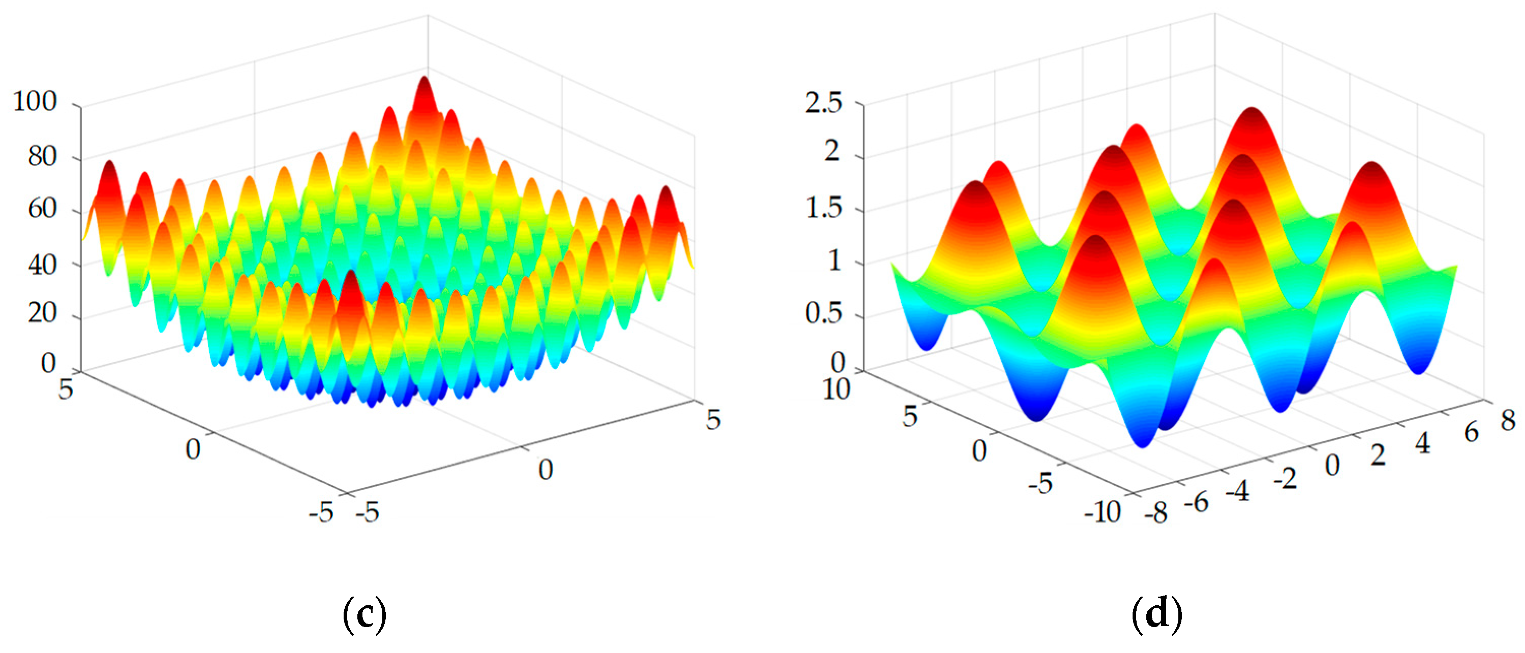
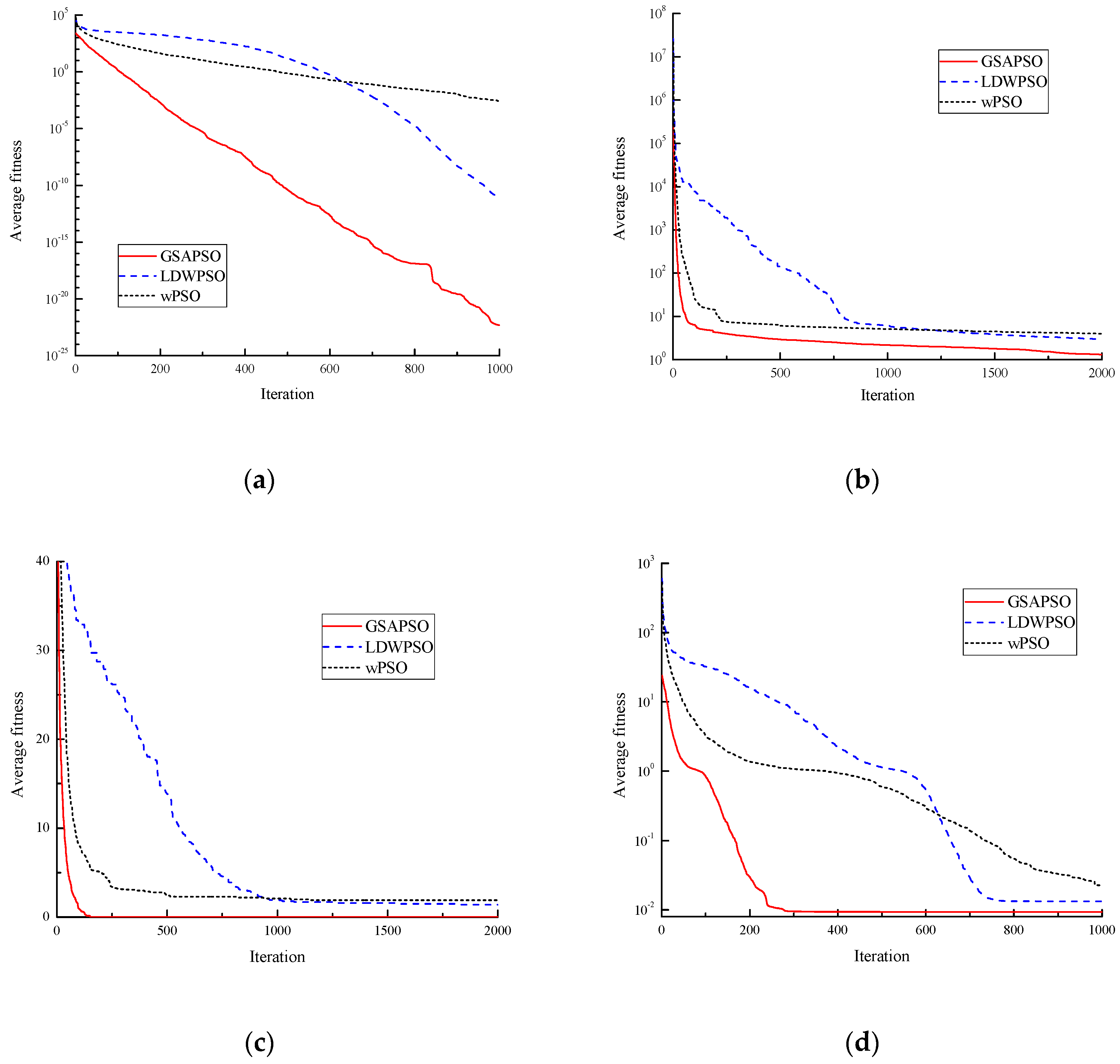
The average adaptation curves of the four standard test functions using the three PSO algorithms are shown in Figure 2.

From Figure 2, it shows that the GSAPSO algorithm had greatly improved on convergence accuracy and convergence time compared to the LDWPSO and WPSO algorithms, which increased the chance of finding the optimal value for the actual optimization problem.

5. Problem Formulations

5.1. Objective Functions

Minimizing the active power losses and maintaining voltage stability are the purposes of the RPO to power system. The bus voltage and the reactive power of the generators both had a certain range of limits, which also would have had an impact on the results at the same time, so the two state variables were added to the objective function as quadratic penalty terms. The RPO problem was formulated as:

$$\min f=\min P_{loss}={\displaystyle \sum _{i,j\in N_B}{g}_{ij}(U_i^2+U_j^2-2U_i{U}_j\cos {\theta }_{ij})}+{\lambda }_1{{\displaystyle \sum _{i=1}^{N_{PQ}}(\frac{U_i-U_{i\lim }}{U_{i\max }-U_{i\min }})}}^2+{\lambda }_2{{\displaystyle \sum _{i=1}^{N_{PV}}(\frac{Q_{Gi}-{Q_G}_{i,\lim }}{Q_{Gi,\max }-Q_{Gi,\min }})}}^2$$

(12)

where U_i is the voltage magnitude at bus i. N_B, N_PQ, N_PV are the total of buses, the set of PQ buses and the set of PV buses respectively. λ₁, λ₂ are the penalty terms, which are assigned according to respective importance of variables. In this paper, it was assumed λ₁ = 100, λ₂ = 10. g_ij, θ_ij were the mutual conductance and voltage angle difference between bus i and j. U_ilim, Q_Gi,lim in Equation (12) was defined as follows:

$$U_{i\lim }=\{\begin{array}{ll}{U}_{i\max },& U_i>U_{i\max }\\ U_{i\min },& U_i<U_{i\min }\end{array}$$

(13)

$$Q_{Gi,\lim }=\{\begin{array}{ll}{Q}_{Gi,\max },& Q_{Gi}>Q_{Gi,\max }\\ Q_{Gi,\min },& Q_{Gi}<Q_{Gi,\min }\end{array}$$

(14)

5.2. Constraints

The constraints were segmented into two parts, which are described as follows:

Equality constraints:

$$\{\begin{array}{ll}{P}_i=U_i{\displaystyle \sum _{j=1}^{N_B}{U}_j(G_{ij}\cos {\theta }_{ij}+B_{ij}\sin {\theta }_{ij})}& i\in N_{PV},N_{PQ}\\ Q_i=U_i{\displaystyle \sum _{j=1}^{N_B}{U}_j(G_{ij}\sin {\theta }_{ij}-B_{ij}\cos {\theta }_{ij})}& i\in N_{PQ}\end{array}$$

(15)

Inequality constraints (control variables):

$$\{\begin{array}{ll}{U}_{Gi,\min }\le U_{Gi}\le U_{Gi,\max },& i\in N_G\\ Q_{Ci,\min }\le Q_{Ci}\le Q_{Ci,\max },& i\in N_C\\ T_{k,\min }\le T_k\le T_{k,\max },& k\in N_T\end{array}$$

(16)

where N_G, N_C, N_T are the quantity of generators, capacitor banks and transformers respectively. U_Gi is the voltage magnitude at generator bus i. Q_Ci is the compensation capacity of ith shunt capacitor; T_k is the tap position of kth transformer.

The inequality constraints on state variables were as follows:

$$\{\begin{array}{ll}{U}_{i,\min }\le U_i\le U_{i,\max }& i\in N_{PQ}\\ Q_{Gi,\min }\le Q_{Gi}\le Q_{Gi,\max }& i\in N_G\end{array}$$

(17)

where Q_Gi is the reactive power of ith generator; U_imin, U_imax, Q_Gi,min, Q_Gi,max are the minimum and maximum of the corresponding variables respectively.

6. GSAPSO Algorithm for RPO

6.1. Treatment of Control Variables

The voltage of the generator is a continuous variable, the transformer tap position and the capacity of capacitor banks are discrete variables. Continuous variables were encoded in real numbers, and integers were applied to encode discrete variables in this paper.

$$X=[U_G;T;C]=[U_{G1},\cdot \cdot \cdot ,U_{Gi},\cdot \cdot \cdot U_{GN};T_1,\cdot \cdot \cdot ,T_i,\cdot \cdot \cdot T_M;C_1,\cdot \cdot \cdot ,C_i,\cdot \cdot \cdot C_K]$$

(18)

where X is individual position of particles; U_Gi is the voltage magnitude of the ith generator. T_i is the tap ratio of ith transformer. C_i is the capacity of ith capacitor banks. The subscripts N, M, and K represent the quantity of generator buses, adjustable transformers, and compensation buses, respectively.

6.2. Treatment of Discrete Variables

This study uses the rounding method to process discrete variables. Their formulas are:

$$\begin{array}{l}{T}_i=round(rand\times stepT)\times T_{step}+T_{\min }\\ Q_{C,i}=round(rand\times step{Q}_C)\times Q_{C,step}+Q_{C,\min }\end{array}$$

(19)

where round(·) is the rounding function; stepT, stepQ_C are the value of tap positions and capacitor banks, respectively; T_step, Q_C,step are the step size of adjustable transformers and capacitor banks, respectively.

6.3. GSAPSO Algorithm for RPO

Step 1: Initialize parameters (including population size, learning factor, inertia weight range and initial value, the maximum number of iterations, the particle velocity range, control variables and its adjustment range).

Step 2: Divide the population into four parts, and initialize the position and velocity for all the particles.

Step 3: Initialize the power flow calculation parameters and calculate the fitness value of each particle based on the fitness function (Equation (12)), and then update the optimal value of the individual and population.

Step 4: If the better particles appear (for the central particles in the second part or the chaotic particles in the fourth part), replace the poor particles in the first part with them, and update the particles.

Step 5: Update the value of inertia weight using Equations (6) to (9).

Step 6: Update the position and velocity of four part particles for the next generation, according to Equations (1) to (5).

Step 7: Calculate the fitness value of particles, and update the best position of the individual and population.

Step 8: If one of the stopping criteria (maximum iterations or fitness accuracy) is satisfied, the search procedure is stopped, else go to Step 4.

7. Simulation

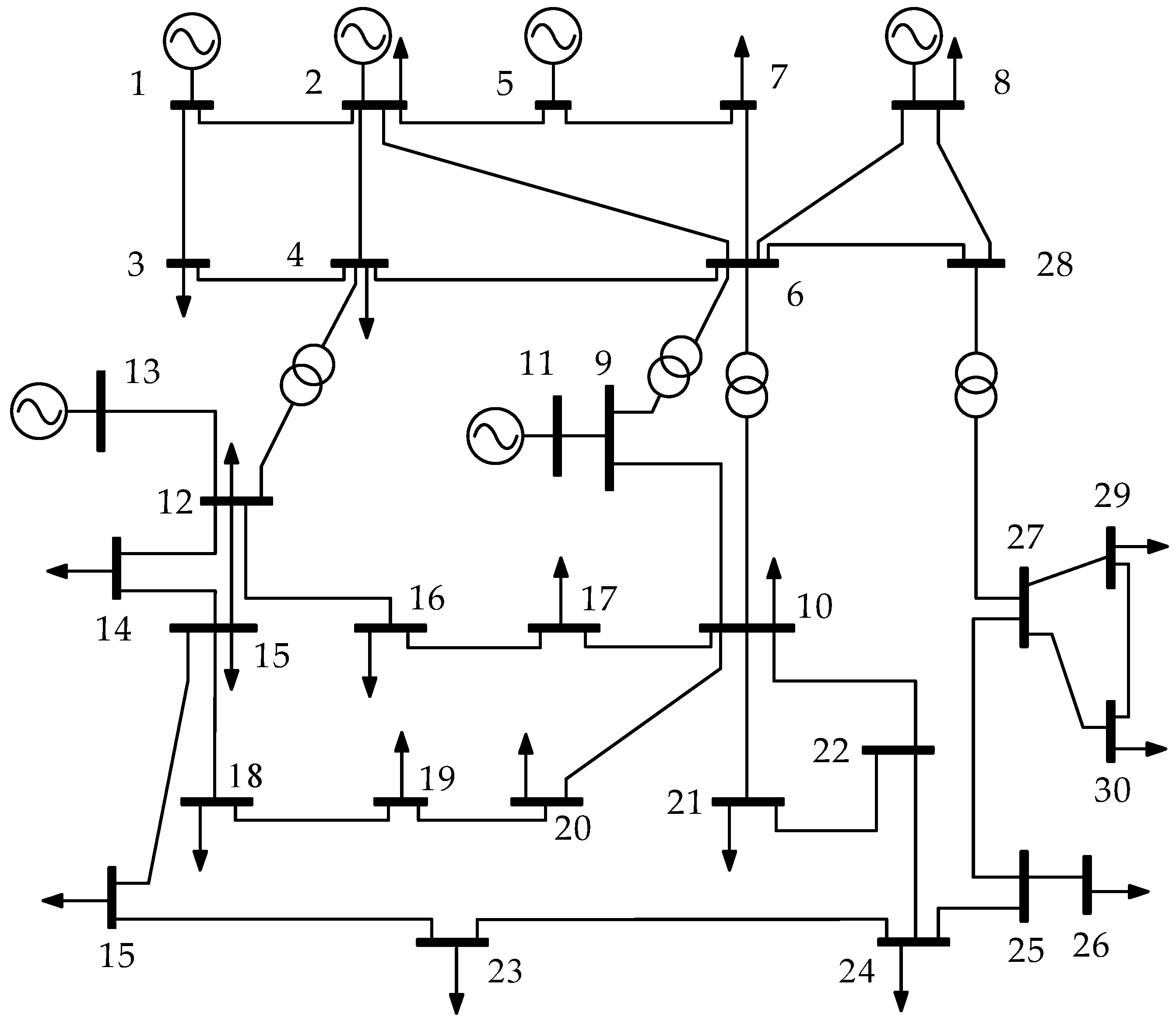
The simulation experiment using standard IEEE 30 bus power system was performed to validate the GSAPSO. Detailed parameters of the system can be found in the literature [31]. The topological structure of it is shown in Figure 3, which consists of six generator buses and four transformers. To the nature of buses, bus 1 was balanced bus, bus 2, 5, 8, 11 and 13 were PV buses, and the other buses were PQ buses. Twelve control variables were involved in optimal reactive power compensation, including six generator voltages, four tap changing transformers, and two shunt compensation capacitor banks. The four branches (6–9, 6–10, 4–12 and 27–28) had transformers with tap changing. In addition, the installation location of shunt compensation capacitor banks were generally ensured at buses 10 and 24 [31]. The reference capacity of the whole power system was 100 MVA and the control variable were set as shown in

Table 4. Control variable setting.

Variables	Minimum (p.u.)	Maximum (p.u.)	Step
UG	0.9	1.1	-
UPQ	0.95	1.05	-
T	0.9	1.1	0.025
C10	0	0.05	0.2
C24	0	0.02	0.2

.

The number of iterations during the calculation period was 100; the other parameter settings were the same with those stated in Section 4.2. Under the initial conditions, the generator voltage and the transformer ratio were both set to 1.0 p.u. When the compensation capacitor capacity was 0 Mvar, the initial network loss was 8.421 MW through the power flow calculation.

For evaluating the performance of GSAPSO for reactive power compensation effectively, the results were compared with PSO, LDWPSO and WPSO. 10 independent trails were carried out and the convergence accuracy took 10⁻⁴. The optimal values, the worst values and the average values of various algorithms were compared. The results are presented in

Table 5. The results with four algorithms.

Optimization Results	PSO	LDWPSO	WPSO	GSAPSO
The optimal value/MW	6.9516	6.824	6.8242	6.8239
The worst value/MW	7.2262	6.8667	6.8614	6.8699
The average value/MW	7.046	6.8342	6.8354	6.8336
The variance	7.034 × 10−3	1.31 × 10−4	1.21 × 10−4	1.17 × 10−4
Iterations of the optimal solution	99	92	77	45
Average iterations	67.3	86.8	67.2	64.6

.

From Table 5, the minimum network loss after the reactive power optimization calculated by the GSAPSO algorithm was 6.8239 MW, the average network loss was 6.8336 MW, the number of optimal solution iterations was 45 and the average number of iterations was 64.6. It demonstrated that the performance of GSAPSO was better than the PSO, LDWPSO and WPSO algorithms. By comparing the variances, we could see that the GSAPSO had a better convergence stability and robustness.

The GSAPSO considered the effective information provided by multiple particles in the optimization process. However, the other three algorithms only considered the role of the optimal individual in the later iteration, so that the algorithms converged slowly near the optimal value. GSAPSO increased the diversity of the population through double central particles, chaotic particles and synergistic particles and jumped out the local optimum value, which enhanced the global optimization ability.

Table 6. The optimized control variables with four optimization algorithms.

Parameters	PSO	LDWPSO	WPSO	GSAPSO
U1	1.0678	1.0686	1.0686	1.0687
U2	1.0453	1.0506	1.0506	1.0506
U5	1.0227	1.0267	1.0267	1.0267
U8	1.0409	1.0381	1.0381	1.0381
U11	1.0026	1.0337	1.0099	1.0363
U13	1.0656	1.0749	1.075	1.0749
C1	40	30	40	30
C2	10	10	10	10
T1	1.025	1.1	1.025	1.05
T2	1.05	0.9	1	0.95
T3	0.975	1	1	1
T4	0.975	0.975	0.975	0.975
Ploss/MW	6.9516	6.824	6.8242	6.8239
Psave/%	17.449	18.964	18.962	18.966

presents the details of control variables after optimization. GSAPSO obtaind the minimum power losses and 18.966% loss reduction, which was better than the other algorithms.

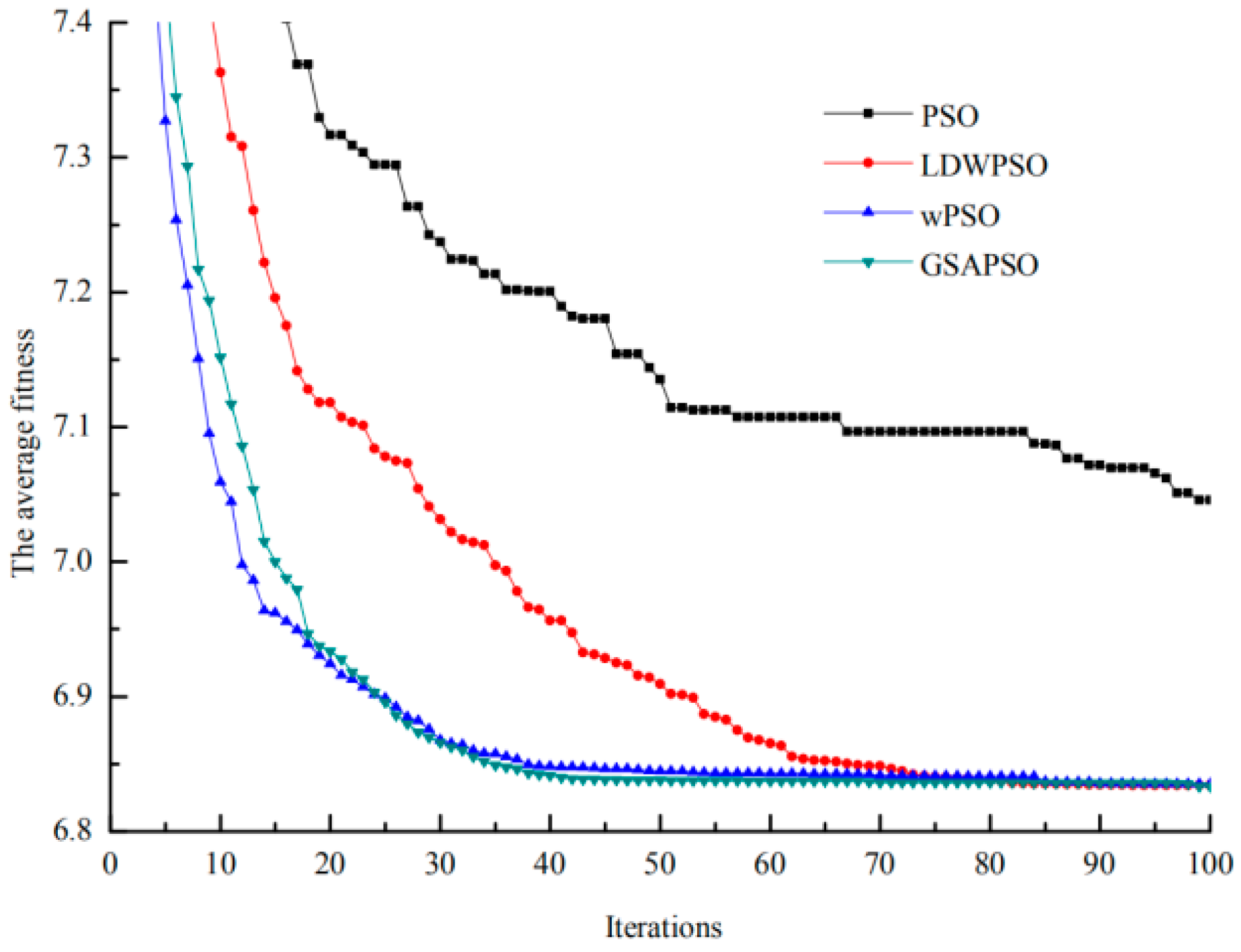
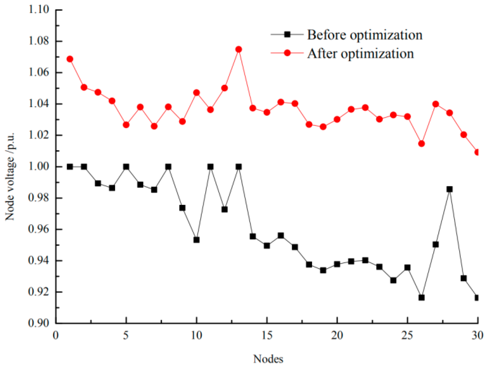
Figure 4 shows the convergence curve of the average fitness value using different algorithms. From Figure 4, it was revealed that GSAPSO performed excellently compared to the other algorithms for the RPO problem. The GSAPSO took around 45 iterations to converge, whereas WPSO, LDWPSO took around 55 iterations and 75 iterations, respectively. The PSO could not converge even after 100 iterations. The voltage magnitudes of buses before and after reactive power optimization are presented in Figure 5.

We can see that the bus voltage magnitudes after reactive power optimization were significantly higher than before optimization. Moreover, they are more stable, the minimum value is 1.0091 p.u. and all values are within the limited range.

8. Conclusions

This paper has presented the GSAPSO, which was proposed by improving the particle update modes and the inertia weight of the algorithm in the iterative process, through which the accuracy and ability of global convergence were effectively improved. The simulation experiments were conducted on four benchmark functions, which validly tested the improved PSO. The salient feature of the improved was that GSAPSO had an obviously higher convergence rate, convergence accuracy and success rate than LDWPSO and WPSO. Then the GSAPSO algorithm was applied for RPO problem on the IEEE30 bus system. The simulation results revealed that the optimal loss reduction rate could reach 18.966%, the optimal solution iteration number was 45 times, which had great improvement compared with 64.6 times, the average iteration number in others algorithms. Moreover, the minimum of bus voltage was 1.0091 p.u. and whole bus voltages were more stable. The proposed GSAPSO algorithm obtained lesser power losses and a more stable voltage compared to the others. The simulation results demonstrated that the GSAPSO had an excellent performance for solving the RPO problems.

References

- Antunes, C.H.; Pires, D.F.; Barrico, C.; Gomes, Á.; Martins, A.G. A Multi-Objective Evolutionary Algorithm for Reactive Power Compensation in Distribution Networks. Appl. Energy 2011, 86, 977–984. [Google Scholar] [CrossRef]
- Ara, A.L.; Kazemi, A.; Gahramani, S.; Behshad, M. Optimal Reactive Power Flow Using Multi-Objective Mathematical Programming. Sci. Iran. 2012, 19, 1829–1836. [Google Scholar]
- Zhang, Y.J.; Ren, Z. Real-Time Optimal Reactive Power Dispatch Using Multi-Agent Technique. Electr. Power Syst. Res. 2004, 69, 259–265. [Google Scholar] [CrossRef]
- Jeyadevi, S.; Baskar, S.; Babulal, C.K.; Iruthayarajan, M.W. Solving Multiobjective Optimal Reactive Power Dispatch Using Modified Nsga-Ii. Int. J. Electr. Power Energy Syst. 2011, 33, 219–228. [Google Scholar] [CrossRef]
- Moghadam, A.; Seifi, A.R. Fuzzy-Tlbo Optimal Reactive Power Control Variables Planning for Energy Loss Minimization. Energy Convers. Manag. 2014, 77, 208–215. [Google Scholar] [CrossRef]
- Borghetti, A. Using Mixed Integer Programming for the Volt/Var Optimization in Distribution Feeders. Electr. Power Syst. Res. 2013, 98, 39–50. [Google Scholar] [CrossRef]
- Mandal, B.; Roy, P.K. Optimal Reactive Power Dispatch Using Quasi-Oppositional Teaching Learning Based Optimization. Int. J. Electr. Power Energy Syst. 2013, 53, 123–134. [Google Scholar] [CrossRef]
- Subbaraj, P.; Rajnarayanan, P.N. Optimal Reactive Power Dispatch Using Self-Adaptive Real Coded Genetic Algorithm. Electr. Power Syst. Res. 2009, 79, 374–381. [Google Scholar] [CrossRef]
- Opoku, G. Optimal Power System Var Planning. IEEE Trans. Power Syst. 1990, 5, 53–60. [Google Scholar] [CrossRef]
- Sun, D.I.; Ashley, B.; Brewer, B.; Hughes, A.; Tinney, W.F. Optimal Power Flow by Newton Approach. IEEE Trans. Power Appar. Syst. 1984, 103, 2864–2880. [Google Scholar] [CrossRef]
- Lo, K.L.; Zhu, S.P. A Decoupled Quadratic Programming Approach for Optimal Power Dispatch. Electr. Power Syst. Res. 1991, 22, 47–60. [Google Scholar] [CrossRef]
- Granville, S. Optimal Reactive Dispatch through Interior Point Methods. IEEE Trans. Power Syst. 1994, 9, 136–146. [Google Scholar] [CrossRef]
- Iba, K. Reactive Power Optimization by Genetic Algorithm. IEEE Trans. Power Syst. 2002, 9, 685–692. [Google Scholar] [CrossRef]
- Mao, Y.; Li, M. Optimal Reactive Power Planning Based on Simulated Annealing Particle Swarm Algorithm Considering Static Voltage Stability. In Proceedings of the 2008 International Conference on Intelligent Computation Technology and Automation (ICICTA), Hunan, China, 20–22 October 2008. [Google Scholar]
- Varadarajan, M.; Swarup, K.S. Differential Evolutionary Algorithm for Optimal Reactive Power Dispatch. Int. J. Electr. Power Energy Syst. 2008, 30, 435–441. [Google Scholar] [CrossRef]
- Varadarajan, M.; Swarup, K.S. Differential Evolution Approach for Optimal Reactive Power Dispatch. Appl. Soft Comput. 2008, 8, 1549–1561. [Google Scholar] [CrossRef]
- Malekpour, A.R.; Tabatabaei, S.; Niknam, T. Probabilistic Approach to Multi-Objective Volt/Var Control of Distribution System Considering Hybrid Fuel Cell and Wind Energy Sources Using Improved Shuffled Frog Leaping Algorithm. Renew. Energy 2012, 39, 228–240. [Google Scholar] [CrossRef]
- Sulaiman, M.H.; Mustaffa, Z.; Mohamed, M.R.; Aliman, O. Using the Gray Wolf Optimizer for Solving Optimal Reactive Power Dispatch Problem. Appl. Soft Comput. 2015, 32, 286–292. [Google Scholar] [CrossRef]
- Singh, R.P.; Mukherjee, V.; Ghoshal, S.P. Optimal Reactive Power Dispatch by Particle Swarm Optimization with an Aging Leader and Challengers. Appl. Soft Comput. 2015, 29, 298–309. [Google Scholar] [CrossRef]
- Niknam, T.; Firouzi, B.B.; Ostadi, A. A New Fuzzy Adaptive Particle Swarm Optimization for Daily Volt/Var Control in Distribution Networks Considering Distributed Generators. Appl. Energy 2010, 87, 1919–1928. [Google Scholar] [CrossRef]
- El-Dib, A.A.; Youssef, H.K.M.; El-Metwally, M.M.; Osman, Z. Optimum Var Sizing and Allocation Using Particle Swarm Optimization. Electr. Power Syst. Res. 2007, 77, 965–972. [Google Scholar] [CrossRef]
- Esmin, A.A.A.; Lambert-Torres, G.; Souza, A.C.Z.D. A Hybrid Particle Swarm Optimization Applied to Loss Power Minimization. IEEE Trans. Power Syst. 2005, 20, 859–866. [Google Scholar] [CrossRef]
- Kennedy, J.; Eberhart, R. Particle swarm optimization. In Proceedings of the IEEE International Conference on Neural Networks, Piscataway, NJ, USA, 27 November–1 December 1995; pp. 1942–1948. [Google Scholar]
- Kannan, S.M.; Renuga, P.; Kalyani, S.; Muthukumaran, E. Optimal Capacitor Placement and Sizing Using Fuzzy-De and Fuzzy-Mapso Methods. Appl. Soft Comput. 2011, 11, 4997–5005. [Google Scholar] [CrossRef]
- Zad, B.B.; Hasanvand, H.; Lobry, J.; Vallée, F. Optimal Reactive Power Control of DGs for Voltage Regulation of MV Distribution Systems Using Sensitivity Analysis Method and PSO Algorithm. Int. J. Electr. Power Energy Syst. 2015, 68, 52–60. [Google Scholar]
- Achayuthakan, C.; Ongsakul, W. TVAC-PSO based optimal reactive power dispatch for reactive power cost allocation under deregulated environment. In Proceedings of the IEEE Conference on Power Energy and Industry Applications, Calgary, AB, Canada, 26–30 July 2009; pp. 1–9. [Google Scholar]
- Vaisakh, K.; Rao, P.K. Optimal reactive power allocation using PSO-DV hybrid algorithm. In Proceedings of the India Conference, Kanpur, India, 11–13 December 2008. [Google Scholar]
- Tang, K.Z.; Liu, B.X. Double Center Particle Swarm Optimization Algorithm. J. Comput. Res. Dev. 2012, 49, 1086–1094. [Google Scholar]
- Arasomwan, M.A.; Adewumi, A.O. On the Performance of Linear Decreasing Inertia Weight Particle Swarm Optimization for Global Optimization. Sci. World J. 2013, 2013, 1–12. [Google Scholar] [CrossRef] [PubMed]
- Ren, Z.H.; Wang, J. New Adaptive Particle Swarm Optimization Algorithm with Dynamically Changing Inertia Weight. Comput. Sci. 2009, 36, 227–229. [Google Scholar]
- Lee, K.Y.; Park, Y.M.; Ortiz, J.L. A United Approach to Optimal Real and Reactive Power Dispatch. IEEE Power Eng. Rev. 2010, PER–5, 42–43. [Google Scholar]
Figure 1.
Three-dimensional map of the four functions: (a) Sphere function; (b) Rosenbrock function; (c) Rastrigin function; (d) Griewank function.
Figure 2.
Function fitness curve: (a) Sphere fitness curve; (b) Rosenbrock fitness curve; (c) Rastrigin fitness curve; (d) Griewank fitness curve.
Figure 3.
IEEE 30 bus power system.
Figure 4.
Convergence curves of average fitness using different algorithms.
Figure 5.
The bus voltage before and after optimization.