Steady-State Modeling of Fuel Cells Based on Atom Search Optimizer

Abstract

In simulation studies, the precision of fuel cell models has a vital role in the quality of results. Unfortunately, due to the shortage of manufacturer data given in the datasheets, several unknown parameters should be defined to establish the fuel cell model for further precise analysis. This research addresses a novel application of the atom search optimization (ASO) algorithm to generate these unknown parameters of the fuel cell model and in particular of the polymer exchange membrane (PEM) type. The objective of this study is to establish an accurate model of the PEM fuel cells, which will provide accurate results of modeling and simulation in a steady-state condition. Simulations and further demonstrations were performed under MATLAB/SIMULINK. The viability of the proposed models was appraised by comparing its simulation results with the experimental results of number of commercial PEM fuel cells. In the same context, the obtained numerical results by the proposed ASO-based method were compared to other challenging optimization methods-based results. Finally, parametric tests were made which indicated the robustness of the ASO results as well. It can be stated here that ASO performs well and has a good capability to extract the unknown parameters with lesser errors.

1. Introduction

Unlike conventional power sources, renewable energy sources as clean energy have received much attention worldwide due to many key reasons, such as the depletion of fossil fuels, price inflations, and other environmental issues. One of the fastest growing and promising renewable energy storage apparatuses is the fuel cell, which can convert fuel chemical energy into electric energy via chemical reactions [1,2,3,4]. Today, many assortments of fuel cells are commercialized, such as the polymer exchange membrane (PEM) type for low-operating temperatures [3], and solid-oxide fuel cells for high-operating temperatures [4,5]. PEM fuel cell stays as an incomparable alternative of importance; specifically, in transportation applications, it plays a role in portable electronic implementations and distributed generators. Moreover, its discriminate properties, such as no dissipated generation, high power density, high efficiency, and low operating pressure and temperature, make PEM fuel cell unequaled [3]. The standard efficiency of PEM fuel cell varies between 30% and 60% dependent on loading condition, and the operating temperatures range from 30 °C to 100 °C [3,4,5,6].

Modeling is highly crucial for better comprehension, analysis, design, simulation, and advancement of high efficiency fuel cells. However, the lack of data, number of obscure parameters, and complication in modeling favor the utilization of optimization algorithms [3]. The majority of deterministic optimization algorithms have their respective limits, like sensitivity to initial values, and fail to provide dependable results. To ameliorate the accuracy of the PEM fuel cells model parameter estimation, many global optimization algorithms have been used. The results obtained using these algorithms are better than those obtained using traditional methods [6].

Many researchers have endeavored to model PEM fuel cell characteristics using many heuristic based optimization algorithms [7,8,9,10,11,12,13,14,15,16,17,18]—in particular, the salp swarm optimizer [7], adaptive ribonucleic acid genetic algorithm (ARNA-GA) [8], genetic algorithm [9,10,11], particle swarm optimizer [12], Taguchi method and genetic algorithm neural networks [13], bird mating optimization algorithm [14], seeker optimizer [15], eclectic hybrid stochastic plan [16], adaptive differential evolution (ADE) algorithm [17], and innovated global harmony search (IGHS) algorithm [18].

Other recent similar optimizers, such as biogeography accompanied by mutation (BBO-M) [19], the simplified teaching-learning based optimizer (STLBO) [20], transmitted adapting differential evolution (TRADE) algorithm [21], hybrid adapting differential evolution (HADE) algorithm [22], nonlinear globally linearizing controller based on an estimator [23], multiverse optimizer (MVO) [24], grasshopper optimization algorithm (GOA) [25], and grey wolf optimizer (GWO) [26], are applied to define the model unknown parameters. In [27], a novel bio-inspired P systems-based optimization algorithm (BIPOA) was introduced to generate the obscure parameters of PEM fuel cells models.

Recently, atom search optimization (ASO), which was developed in 2019, has been utilized in hydro-geologic coefficient estimation [28] and dispersion parameter estimation [29]. In agreement with the no-free lunch theorem, several optimization techniques should be assessed to solve specific problems with attempts to get near/close to optimal solutions. Therefore, ASO is quoted in this current research because its reported results are promising and prove that ASO is superior to other algorithms in parameter estimation [28,29].

In this paper, ASO was used to generate the obscure parameters of two commercial PEM fuel cells. Further validations and comparisons were made to indicate the performance of the proposed ASO-based methodology. The crucial contributions of this research include execution of a novel algorithm, namely ASO, to generate the obscure parameters of the PEM fuel cell model in comparison to other competing methods recently reported in the literature, as well as proving the possibility of benefiting from ASO to optimize several complicated problems in engineering.

The paper is organized as follows: Section 1 gives a brief introduction and survey in this regard. Section 2 illustrates the mathematical modeling of PEM fuel cells. In Section 3, the adapted objective function and constraints are revealed. The ASO procedures are explained in Section 4. Section 5 discusses the obtained results, along with necessary validations. Conclusions are drawn in Section 6. Finally, acknowledgements, conflicts of interest, and authors’ contributions are presented.

2. Mathematical Modeling of PEM Fuel Cell

The model of a PEM fuel cell stack was intensively demonstrated in the literature. For a stack consisting of ${\mathrm{n}}_{\mathrm{cells}}$ series connected cells, the stack’s terminal voltage ${\mathrm{V}}_{\mathrm{stack}}$ can be evaluated by the following equation [9,25]:

$${\mathrm{V}}_{\mathrm{stack}}={\mathrm{n}}_{\mathrm{cells}}·\left(\mathrm{E}-{\mathrm{V}}_{\mathrm{act}}-{\mathrm{V}}_{\Omega }-{\mathrm{V}}_{\mathrm{con}}\right).$$

(1)

By assuming that the ${\mathrm{H}}_2$ flow rate is controllable with regard to the loading condition, it can be revealed that the utilization factor is constant and has a typical value of 95% [25]. ${\mathrm{E}}_{\max }$ is the maximum voltage that can be generated by the PEM fuel cell at a higher heating value of ${\mathrm{H}}_2$, which typically equals 1.48 V/cell [25]. It is of value to emphasize that the theoretical voltage with respect to the lower heating value is 1.23 V/cell (See (2)). The aforementioned variables indicated in (1) are stated as follows:

$$\mathrm{E}=1.299-0.85·{10}^{-3}\left({\mathrm{T}}_{\mathrm{fc}}-298.15\right)+4.3085·{10}^{-5}{\mathrm{T}}_{\mathrm{fc}}\ln \left({\mathrm{P}}_{{\mathrm{H}}_2}\sqrt{{\mathrm{P}}_{{\mathrm{O}}_2}}\right),$$

(2)

$${\mathrm{P}}_{{\mathrm{H}}_2}=\frac{{\mathrm{RH}}_{\mathrm{a}}·{\mathrm{P}}_{{\mathrm{H}}_2\mathrm{O}}}{2}\left[1/\left(\frac{{\mathrm{RH}}_{\mathrm{a}}·{\mathrm{P}}_{{\mathrm{H}}_2\mathrm{O}}}{{\mathrm{P}}_{\mathrm{a}}}·{\mathrm{e}}^{\frac{1.635{\mathrm{i}}_{\mathrm{fc}}/\mathrm{A}}{{\mathrm{T}}_{\mathrm{fc}}^{1.334}}}\right)-1\right],$$

(3)

$${\mathrm{P}}_{{\mathrm{O}}_2}=\frac{{\mathrm{RH}}_{\mathrm{c}}·{\mathrm{P}}_{{\mathrm{H}}_2\mathrm{O}}}{2}\left[1/\left(\frac{{\mathrm{RH}}_{\mathrm{c}}·{\mathrm{P}}_{{\mathrm{H}}_2\mathrm{O}}}{{\mathrm{P}}_{\mathrm{C}}}·{\mathrm{e}}^{\frac{4.192{\mathrm{i}}_{\mathrm{fc}}/\mathrm{A}}{{\mathrm{T}}_{\mathrm{fc}}^{1.334}}}\right)-1\right],$$

(4)

$$\begin{gathered} {\mathrm{P}}_{{\mathrm{H}}_2\mathrm{O}}=2.95·{10}^{-2}{\mathrm{T}}_{\mathrm{c}}-9.18·{10}^{-5}{\mathrm{T}}_{\mathrm{c}}^2+1.44·{10}^{-7}{\mathrm{T}}_{\mathrm{c}}^3-2.18, \\ {\mathrm{T}}_{\mathrm{c}}={\mathrm{T}}_{\mathrm{fc}}-273.15, \end{gathered}$$

(5)

$${\mathrm{V}}_{\mathrm{act}}=-\left[{\mathsf{\xi }}_1+{\mathsf{\xi }}_2{\mathrm{T}}_{\mathrm{fc}}+{\mathsf{\xi }}_3{\mathrm{T}}_{\mathrm{fc}}\ln \left({\mathrm{C}}_{{\mathrm{O}}_2}\right)+{\mathsf{\xi }}_4{\mathrm{T}}_{\mathrm{fc}}\ln \left({\mathrm{I}}_{\mathrm{fc}}\right)\right],$$

(6)

$${\mathrm{C}}_{{\mathrm{O}}_2}=\frac{{\mathrm{P}}_{{\mathrm{O}}_2}}{5.08·{10}^6}·{\mathrm{e}}^{-\frac{498}{{\mathrm{T}}_{\mathrm{fc}}}},$$

(7)

$$\begin{gathered} {\mathrm{V}}_{\Omega }={\mathrm{I}}_{\mathrm{fc}}\left({\mathrm{R}}_{\mathrm{m}}+{\mathrm{R}}_{\mathrm{C}}\right);{\mathrm{R}}_{\mathrm{m}}=\frac{{\mathsf{\rho }}_{\mathrm{m}}\mathrm{l}}{\mathrm{A}}, \\ {\mathsf{\rho }}_{\mathrm{m}}=\frac{181.6\left[1+0.03\left(\frac{{\mathrm{I}}_{\mathrm{fc}}}{\mathrm{A}}\right)+0.062{\left(\frac{{\mathrm{T}}_{\mathrm{fc}}}{303}\right)}^2{\left(\frac{{\mathrm{I}}_{\mathrm{fc}}}{\mathrm{A}}\right)}^{2.5}\right]}{\left[\mathsf{\Psi }-0.634-3\left(\frac{{\mathrm{I}}_{\mathrm{fc}}}{\mathrm{A}}\right)\right]{\mathrm{e}}^{4.18·\frac{{\mathrm{T}}_{\mathrm{fc}}-303}{{\mathrm{T}}_{\mathrm{fc}}}}}, \end{gathered}$$

(8)

$${\mathrm{V}}_{\mathrm{con}}=-\mathrm{b}·\ln \left(\frac{{\mathrm{J}}_{\max }-\mathrm{J}}{{\mathrm{J}}_{\max }}\right).$$

(9)

The power of the PEM fuel cell stack $\left({\mathrm{P}}_{\mathrm{stack}}\right)$ is stated as defined in (10):

$${\mathrm{P}}_{\mathrm{stack}}={\mathrm{V}}_{\mathrm{stack}}·{\mathrm{I}}_{\mathrm{fc}}.$$

(10)

According to Equations (1) to (9), it is obvious that seven coefficients $\left({\mathsf{\xi }}_1,{\mathsf{\xi }}_2,{\mathsf{\xi }}_3,{\mathsf{\xi }}_4,\mathsf{\Psi },{\mathrm{R}}_{\mathrm{C}},\mathrm{and}\mathrm{b}\right)$ need to be identified. These parameters are not predetermined in the manufacturer's datasheet. ASO is utilized in optimizing the seven coefficients to own finest values inside their higher and lower limits. Optimization is performed to ensure a precise modeling of PEM fuel cell under study and simulation.

3. Formulating the Objective Function and Constraints

Minimizing the sum of the squared error (SSE) between the computed voltage (${\mathrm{V}}_{\mathrm{com}}$) and measured voltage (${\mathrm{V}}_{\mathrm{meas}}$) is the objective function (OF) for the modeling of PEM fuel cell, as revealed in (11).

$$\mathrm{OF}=\min \left(\mathrm{SSE}\right)=\min \left({\displaystyle \sum }_{\mathrm{k}=1}^{\mathrm{M}}{\left[{\mathrm{V}}_{\mathrm{com}}\left(\mathrm{k}\right)-{\mathrm{V}}_{\mathrm{meas}}\left(\mathrm{k}\right)\right]}^2\right)$$

(11)

The OF is subjected to constraints that are determined by the lower and upper limits of $\left({\mathsf{\xi }}_1,{\mathsf{\xi }}_2,{\mathsf{\xi }}_3,{\mathsf{\xi }}_4,\mathsf{\Psi },{\mathrm{R}}_{\mathrm{C}},\mathrm{and}\mathrm{b}\right)$.

Minimizing the mean squared error (MSE) represents the OF in some previous studies. To compare the obtained numerical results by ASO with other challenging optimization methods-based results, MSE can be computed as depicted in (12):

$$\mathrm{MSE}=\frac{\mathrm{SSE}}{\mathrm{M}}.$$

(12)

4. Atom Search Optimizer (ASO)

Atoms, basic building blocks of all materials, are moving continuously, and their motions are governed by the classical mechanics [30]. Assume that force of interaction is ${\mathrm{F}}_{\mathrm{i}}$ and force of constraint is ${\mathrm{G}}_{\mathrm{i}}$, and they are applied together on the atom i inside an atom arrangement. Subsequently, the relationship between acceleration ${\mathrm{a}}_{\mathrm{i}}$ and mass m_i of atom is derived by the second law of Newton’s laws as shown in (13) [29,30]:

$${\mathrm{a}}_{\mathrm{i}}=\frac{{\mathrm{F}}_{\mathrm{i}}+{\mathrm{G}}_{\mathrm{i}}}{{\mathrm{m}}_{\mathrm{i}}}.$$

(13)

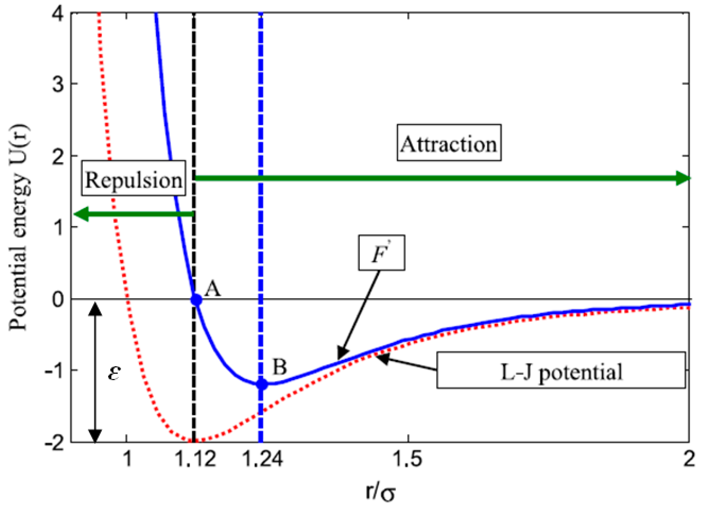
At iteration t, the atom i is exposed to interaction force by the atom j in the dimension d and is written using the Lennard–Jones (L–J) potential as [29,30]:

$${\mathrm{F}}_{\mathrm{ij}}^{\mathrm{d}}\left(\mathrm{t}\right)=\frac{24\mathsf{\epsilon }\left(\mathrm{t}\right)}{\mathsf{\sigma }\left(\mathrm{t}\right)}\left[{\left(\frac{\mathsf{\sigma }\left(\mathrm{t}\right)}{{\mathrm{r}}_{\mathrm{ij}}\left(\mathrm{t}\right)}\right)}^{13}-{\left(\frac{\mathsf{\sigma }\left(\mathrm{t}\right)}{{\mathrm{r}}_{\mathrm{ij}}\left(\mathrm{t}\right)}\right)}^7\right]\frac{{\mathrm{r}}_{\mathrm{ij}}\left(\mathrm{t}\right)}{{\mathrm{r}}_{\mathrm{ij}}^{\mathrm{d}}\left(\mathrm{t}\right)},$$

(14)

and:

$${\mathrm{F}}_{\mathrm{ij}}^{\prime }\left(\mathrm{t}\right)=\frac{24\mathsf{\epsilon }\left(\mathrm{t}\right)}{\mathsf{\sigma }\left(\mathrm{t}\right)}\left[{\left(\frac{\mathsf{\sigma }\left(\mathrm{t}\right)}{{\mathrm{r}}_{\mathrm{ij}}\left(\mathrm{t}\right)}\right)}^{13}-{\left(\frac{\mathsf{\sigma }\left(\mathrm{t}\right)}{{\mathrm{r}}_{\mathrm{ij}}\left(\mathrm{t}\right)}\right)}^7\right].$$

(15)

Figure 1 shows the interaction force of atoms against the spacing between atoms. The repulsion is positive, and the attraction is negative; therefore, atoms would not be converging to a certain location. Equation (15) cannot be utilized straightway in optimization, so it can be adapted as:

$${\mathrm{F}}_{\mathrm{ij}}^{\prime }\left(\mathrm{t}\right)=-\mathsf{\eta }\left(\mathrm{t}\right)\left[2{\left({\mathrm{h}}_{\mathrm{ij}}\left(\mathrm{t}\right)\right)}^{13}-{\left({\mathrm{h}}_{\mathrm{ij}}\left(\mathrm{t}\right)\right)}^7\right],$$

(16)

$${\mathrm{h}}_{\mathrm{ij}}\left(\mathrm{t}\right)=\frac{\mathsf{\sigma }\left(\mathrm{t}\right)}{{\mathrm{r}}_{\mathrm{ij}}\left(\mathrm{t}\right)}.$$

(17)

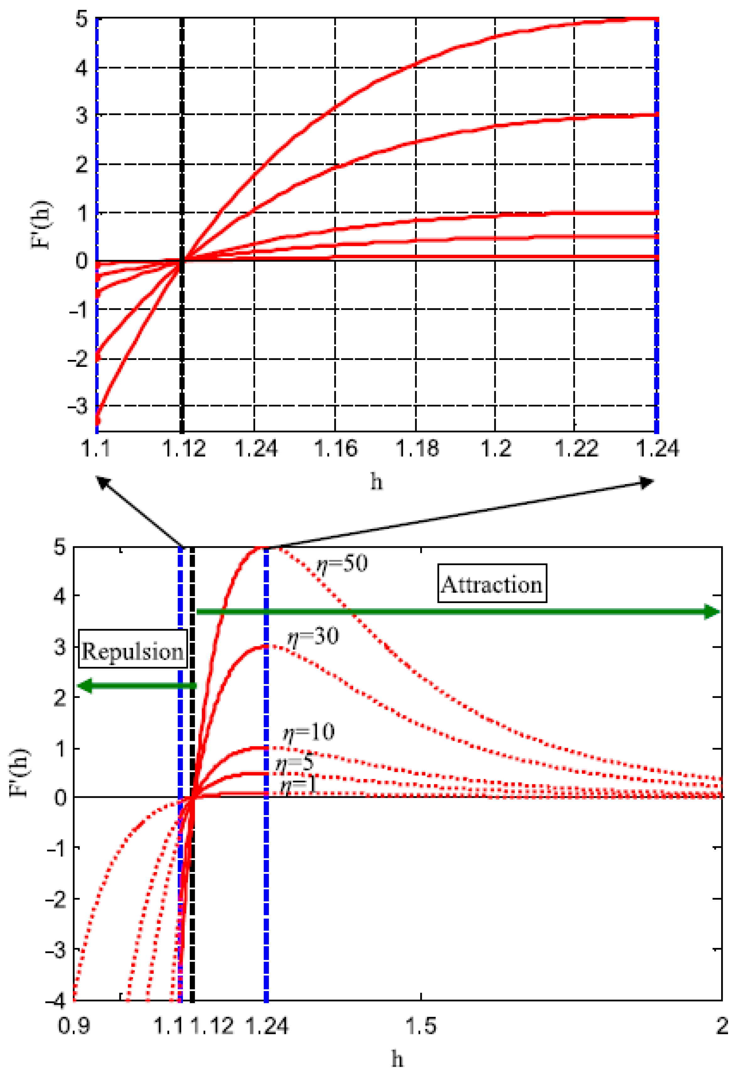
The deepness function is used to set the attraction zone or the repulsion zone that is stated as [28]:

$$\mathsf{\eta }\left(\mathrm{t}\right)=\mathsf{\alpha }{\left(1-\frac{\mathrm{t}-1}{\mathrm{T}}\right)}^3{\mathrm{e}}^{-\frac{20\mathrm{t}}{\mathrm{T}}}.$$

(18)

Figure 2 demonstrates F′ against η when h varies between 0.9 and 2. The attraction happens while h is varying from 1.12 to 2, the repulsion happens while h is varying between 0.9 and 1.12, and the equilibrium happens while h equals 1.12. Consequently, in ASO, to ameliorate the reconnaissance, repulsion has a lower limit while F′ has a lesser value at which h = 1.1, and attraction has an upper limit while F′ has a bigger value at which h = 1.24; thus, h is stated as:

$${\mathrm{h}}_{\mathrm{ij}}\left(\mathrm{t}\right)=\{\begin{array}{c}{\mathrm{h}}_{\min }\\ \frac{{\mathrm{r}}_{\mathrm{ij}}\left(\mathrm{t}\right)}{\mathsf{\sigma }\left(\mathrm{t}\right)}\\ {\mathrm{h}}_{\max }\end{array}\begin{array}{c}\frac{{\mathrm{r}}_{\mathrm{ij}}\left(\mathrm{t}\right)}{\mathsf{\sigma }\left(\mathrm{t}\right)}<{\mathrm{h}}_{\min }\\ {\mathrm{h}}_{\min }\le \frac{{\mathrm{r}}_{\mathrm{ij}}\left(\mathrm{t}\right)}{\mathsf{\sigma }\left(\mathrm{t}\right)}\le {\mathrm{h}}_{\max }\\ \frac{{\mathrm{r}}_{\mathrm{ij}}\left(\mathrm{t}\right)}{\mathsf{\sigma }\left(\mathrm{t}\right)}>{\mathrm{h}}_{\max }\end{array},$$

(19)

σ(t) is stated as:

$$\mathsf{\sigma }\left(\mathrm{t}\right)=\Vert {\mathrm{x}}_{\mathrm{ij}}\left(\mathrm{t}\right),\frac{{\sum }_{\mathrm{j}\in \mathrm{Kbest}}{\mathrm{x}}_{\mathrm{ij}}\left(\mathrm{t}\right)}{\mathrm{K}\left(\mathrm{t}\right)}{\Vert }_2,$$

(20)

and:

$$\{\begin{array}{c}{\mathrm{h}}_{\min }={\mathrm{g}}_0+\mathrm{g}\left(\mathrm{t}\right)\\ {\mathrm{h}}_{\max }=\mathrm{u}\end{array}.$$

(21)

Consequently, u and ${\mathrm{g}}_0$ are equal to 1.24 and 1.1, consecutively. g symbolizes the drift factor that may transport the procedure from the reconnaissance to the profiteering, which is stated as:

$$\mathrm{g}\left(\mathrm{t}\right)=0.1\times \sin \left(\frac{\mathsf{\pi }}{2}\times \frac{\mathrm{t}}{\mathrm{T}}\right).$$

(22)

Afterwards, total force applied on the atom i by other atoms is the summation of weighted components in the d-th dimension that is depicted in (23):

$${\mathrm{F}}_{\mathrm{i}}^{\mathrm{d}}\left(\mathrm{t}\right)={{\displaystyle \sum }}_{\mathrm{j}\in {\mathrm{K}}_{\mathrm{best}}}{\mathrm{rand}}_{\mathrm{j}}.{\mathrm{F}}_{\mathrm{ij}}^{\mathrm{d}}\left(\mathrm{t}\right).$$

(23)

From the third law of Newton’s laws:

$${\mathrm{F}}_{\mathrm{ij}}=-{\mathrm{F}}_{\mathrm{ji}}.$$

(24)

Molecular dynamics put a geometric constraint that acts a serious task in the atom movement. In ASO, assume that the best atom owns a covalence bond with each atom; therefore, a constraint force is exerted on each atom by the best atom. Hence, the atom i constraint is modified as:

$${\mathsf{\theta }}_{\mathrm{i}}\left(\mathrm{t}\right)=\left[{\left|x_{\mathrm{i}}\left(\mathrm{t}\right)-x_{\mathrm{best}}\left(\mathrm{t}\right)\right|}^2-{\mathrm{b}}_{\mathrm{i},\mathrm{best}}^2\right].$$

(25)

Therefore, the force of constraint is stated as [29,30]:

$${\mathrm{G}}_{\mathrm{i}}^{\mathrm{d}}\left(\mathrm{t}\right)=-\mathsf{\lambda }\left(\mathrm{t}\right)\nabla {\mathsf{\theta }}_{\mathrm{i}}^{\mathrm{d}}\left(\mathrm{t}\right)=-2\mathsf{\lambda }\left(\mathrm{t}\right)\left({\mathrm{x}}_{\mathrm{i}}^{\mathrm{d}}\left(\mathrm{t}\right)-{\mathrm{x}}_{\mathrm{best}}^{\mathrm{d}}\left(\mathrm{t}\right)\right).$$

(26)

By replacement of 2λ with λ:

$${\mathrm{G}}_{\mathrm{i}}^{\mathrm{d}}\left(\mathrm{t}\right)=\mathsf{\lambda }\left(\mathrm{t}\right)\left({\mathrm{x}}_{\mathrm{best}}^{\mathrm{d}}\left(\mathrm{t}\right)-{\mathrm{x}}_{\mathrm{i}}^{\mathrm{d}}\left(\mathrm{t}\right)\right).$$

(27)

The Lagrange multiplier is stated as:

$$\mathsf{\lambda }\left(\mathrm{t}\right)=\mathsf{\beta }.exp\left(-\frac{20\mathrm{t}}{\mathrm{T}}\right).$$

(28)

Consequently, the atom i acceleration at iteration t $\left({\mathrm{a}}_{\mathrm{i}}^{\mathrm{d}}\left(\mathrm{t}\right)\right)$ is stated as:

$$\begin{gathered} {\mathrm{a}}_{\mathrm{i}}^{\mathrm{d}}\left(\mathrm{t}\right)=\frac{{\mathrm{F}}_{\mathrm{i}}^{\mathrm{d}}\left(\mathrm{t}\right)}{{\mathrm{m}}_{\mathrm{i}}^{\mathrm{d}}\left(\mathrm{t}\right)}+\frac{{\mathrm{G}}_{\mathrm{i}}^{\mathrm{d}}\left(\mathrm{t}\right)}{{\mathrm{m}}_{\mathrm{i}}^{\mathrm{d}}\left(\mathrm{t}\right)}=-\mathsf{\alpha }{\left(1-\frac{\mathrm{t}-1}{\mathrm{T}}\right)}^3{\mathrm{e}}^{-\frac{20\mathrm{t}}{\mathrm{T}}}, \\ {\sum }_{\mathrm{j}\in \mathrm{Kbest}}\frac{{\mathrm{rand}}_{\mathrm{j}}\left[2\times {\left({\mathrm{h}}_{\mathrm{ij}}\left(\mathrm{t}\right)\right)}^{13}-{\left({\mathrm{h}}_{\mathrm{ij}}\left(\mathrm{t}\right)\right)}^7\right]}{{\mathrm{m}}_{\mathrm{i}}\left(\mathrm{t}\right)}, \\ \frac{\left({\mathrm{x}}_{\mathrm{i}}^{\mathrm{d}}\left(\mathrm{t}\right)-{\mathrm{x}}_{\mathrm{j}}^{\mathrm{d}}\left(\mathrm{t}\right)\right)}{\Vert x_i\left(\mathrm{t}\right)-x_j\left(\mathrm{t}\right){\Vert }_2}+{\mathsf{\beta }\mathrm{e}}^{-\frac{20\mathrm{t}}{\mathrm{T}}}\frac{{\mathrm{x}}_{\mathrm{best}}^{\mathrm{d}}\left(\mathrm{t}\right)-{\mathrm{x}}_{\mathrm{i}}^{\mathrm{d}}\left(\mathrm{t}\right)}{{\mathrm{m}}_{\mathrm{i}}\left(\mathrm{t}\right)}. \end{gathered}$$

(29)

If the population of atoms is ${\mathrm{N}}_{\mathrm{P}}$, the mass of atom i $\left({\mathrm{m}}_{\mathrm{i}}\left(\mathrm{t}\right)\right)$ is computed using (30)–(31):

$${\mathrm{M}}_{\mathrm{i}}\left(\mathrm{t}\right)=\exp \left(-\frac{{\mathrm{Fit}}_{\mathrm{i}}\left(\mathrm{t}\right)-{\mathrm{Fit}}_{\mathrm{best}}\left(\mathrm{t}\right)}{{\mathrm{Fit}}_{\mathrm{worst}}\left(\mathrm{t}\right)-{\mathrm{Fit}}_{\mathrm{best}}\left(\mathrm{t}\right)}\right),$$

(30)

$${\mathrm{m}}_{\mathrm{i}}\left(\mathrm{t}\right)=\frac{{\mathrm{M}}_{\mathrm{i}}\left(\mathrm{t}\right)}{{\sum }_{\mathrm{j}=1}^{{\mathrm{N}}_{\mathrm{P}}}{\mathrm{M}}_{\mathrm{j}}\left(\mathrm{t}\right)}.$$

(31)

In case of minimization, Fit_worst(t) and Fit_best(t) are the maximum and the minimum fitness values of atoms at the iteration t, consecutively. Fit_i(t) is the function fitness value of the atom i at the iteration t. ${\mathrm{Fit}}_{\mathrm{worst}}\left(t\right)$ and ${\mathrm{Fit}}_{\mathrm{best}}\left(t\right)$ are expressed in (32) and (33), respectively:

$${\mathrm{Fit}}_{\mathrm{worst}}\left(t\right)={\max }_{\mathrm{i}\in \left\{1,2,\dots .,{\mathrm{N}}_{\mathrm{P}}\right\}}{\mathrm{Fit}}_{\mathrm{i}}\left(\mathrm{t}\right),$$

(32)

$${\mathrm{Fit}}_{\mathrm{best}}\left(t\right)={\min }_{\mathrm{i}\in \left\{1,2,\dots .,{\mathrm{N}}_{\mathrm{P}}\right\}}{\mathrm{Fit}}_{\mathrm{i}}\left(\mathrm{t}\right).$$

(33)

For simplification, the velocity and the position of the atom i in the iteration t + 1 is signified as:

$${\mathsf{\upsilon }}_{\mathrm{i}}^{\mathrm{d}}\left(\mathrm{t}+1\right)={\mathrm{rand}}_{\mathrm{i}}^{\mathrm{d}}{\mathsf{\upsilon }}_{\mathrm{i}}^{\mathrm{d}}\left(\mathrm{t}\right)+{\mathrm{a}}_{\mathrm{i}}^{\mathrm{d}}\left(\mathrm{t}\right),$$

(34)

$${\mathrm{x}}_{\mathrm{i}}^{\mathrm{d}}\left(\mathrm{t}+1\right)={\mathrm{x}}_{\mathrm{i}}^{\mathrm{d}}\left(\mathrm{t}\right)+{\mathsf{\upsilon }}_{\mathrm{i}}^{\mathrm{d}}\left(\mathrm{t}+1\right).$$

(35)

In the ASO algorithm, to ameliorate the reconnaissance in earlier iterations, every atom reacts with atoms owning as many better values of fitness as possible. To ameliorate the profiteering in later iterations, every atom reacts with atoms owning as few better values of fitness as possible. K piecemeal decreases as the iterations elapse, and it is computed using the formula stated in (36):

$$\mathrm{K}\left(\mathrm{t}\right)={\mathrm{N}}_{\mathrm{P}}-\left({\mathrm{N}}_{\mathrm{P}}-2\right)\times \sqrt{\mathrm{t}/\mathrm{T}}.$$

(36)

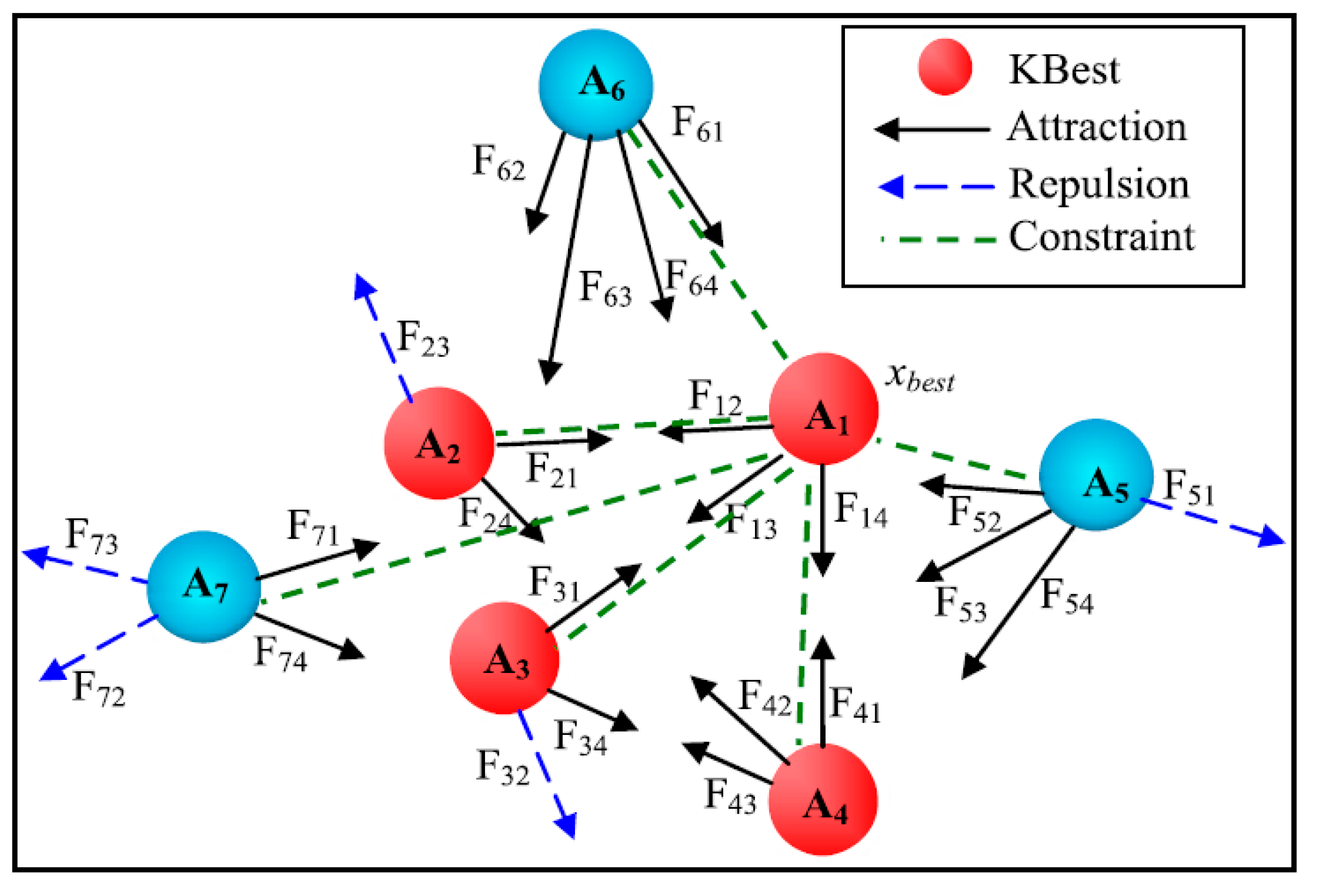
Figure 3 displays the forces in an atom arrangement. The atoms A₁, A₂, A₃, and A₄ have the best values of fitness, so they are considered as the ${\mathrm{K}}_{\mathrm{best}}$. Each atom in the arrangement repels or attracts each other. Each atom in the arrangement, excluding A₁ (${\mathrm{X}}_{\mathrm{best}}$), owns a force of constraint via the best atom A₁.

The computational procedure of the ASO algorithm is as follows:

Step 1: Randomly initialize a set of atoms X (solutions) and their velocity υ, and set ${\mathrm{Fit}}_{\mathrm{best}}$ = ∞, t = 1, i = 1.   Step 2: Increment t = t + 1.   Step 3: Increment i = i + 1.   Step 4: Calculate the fitness value ${\mathrm{Fit}}_{\mathrm{i}}$.   Step 5: If ${\mathrm{Fit}}_{\mathrm{i}}$ ˃ ${\mathrm{Fit}}_{\mathrm{best}}$, set ${\mathrm{Fit}}_{\mathrm{best}}$ = ${\mathrm{Fit}}_{\mathrm{i}}$ and ${\mathrm{X}}_{\mathrm{best}}$ = ${\mathrm{X}}_{\mathrm{i}}$.   Step 6: Calculate the mass ${\mathrm{m}}_{\mathrm{i}}$(t) using Equations (30) and (31).   Step 7: Determine its K neighbors using Equation (36).   Step 8: Calculate the force of interaction Fi and the force of constraint is ${\mathrm{G}}_{\mathrm{i}}$ using Equations (23) and (27), respectively.   Step 9: Update the velocity and the position using Equations (34) and (35), respectively.   Step 10: If i ≤ ${\mathrm{N}}_{\mathrm{p}}$ go to Step 3.   Step 11: If t ≤ T, go to Step 2.   Step 12: Find the best solution so far, ${\mathrm{X}}_{\mathrm{best}}$.   Step 13: Stop.

5. Demonstrated Results, Discussions and Validations

In this section, ASO is utilized to estimate the PEM fuel cell model parameters $\left({\mathsf{\xi }}_1,{\mathsf{\xi }}_2,{\mathsf{\xi }}_3,{\mathsf{\xi }}_4,\mathsf{\Psi },{\mathrm{R}}_{\mathrm{C}},\mathrm{b}\right)$. In this study, two models of marketable PEM fuel cells are tested to legalize the proposed ASO-based methodology in a steady-state condition. The lower and upper limits of $\left({\mathsf{\xi }}_1,{\mathsf{\xi }}_2,{\mathsf{\xi }}_3,{\mathsf{\xi }}_4,\mathsf{\Psi },{\mathrm{R}}_{\mathrm{C}},\mathrm{b}\right)$ exist in literature as follows [20,25,26]:

$$\begin{gathered} -1.1997\le {\mathsf{\xi }}_1\le -0.8532 \\ 0.001\le {\mathsf{\xi }}_2\le 0.005 \\ 3.6·{10}^{-5}\le {\mathsf{\xi }}_3\le 9.8·{10}^{-5} \\ -2.6·{10}^{-4}\le {\mathsf{\xi }}_4\le -9.54·{10}^{-5} \\ 13\le \mathsf{\Psi }\le 23 \\ {10}^{-4}\le {\mathrm{R}}_{\mathrm{C}}\le 8·{10}^{-4} \\ 0.0136\le \mathrm{b}\le 0.5 \end{gathered}$$

(37)

The parameters’ bounds are the same in all test cases to ensure fair comparisons with other challenging optimization methods.

Both ${\mathrm{RH}}_{\mathrm{c}}$ and ${\mathrm{RH}}_{\mathrm{a}}$ are 1. Both ${\mathrm{P}}_{\mathrm{c}}$ and ${\mathrm{P}}_{\mathrm{a}}$ are 1 atm. The maximum iterations are 3000. ASO parameters $\left({\mathrm{N}}_{\mathrm{P}},\mathsf{\alpha },\mathsf{\beta }\right)$ are determined by means of trial and error as other challenging heuristic-based optimization methods as shown in

Table 1. Atom search optimization (ASO) adapted controlling parameters.

ASO Parameters	SR-12 Modular	250 W Stack
$N_P$	25	10
$\mathsf{\alpha }$	40	50
$\mathsf{\beta }$	0.2	0.2

. The finest values of obscure parameters are yielded after executing ASO for some independent runs because of the high haphazardness of such algorithms.

5.1. Test Case 1

In this case, a model of SR-12 500 W modular PEM fuel cell was tested to regularize the performance of ASO. The datasheet was taken from [17,18,21,25,26] as follows: ${\mathrm{n}}_{\mathrm{cells}}=48$, $\mathrm{A}=62.5{\mathrm{cm}}^2$, $\mathrm{l}=0.025\mathrm{mm}$, ${\mathrm{J}}_{\max }=0.672\mathrm{A}/{\mathrm{cm}}^2$, ${\mathrm{T}}_{\mathrm{fc}}=323\mathrm{K}$, ${\mathrm{P}}_{{\mathrm{H}}_2}=1.47628\mathrm{atm}$, ${\mathrm{P}}_{{\mathrm{O}}_2}=0.2095\mathrm{atm}$. Twenty measurements in I–V characteristics of the fuel cell (M = 20) were utilized in optimization using ASO.

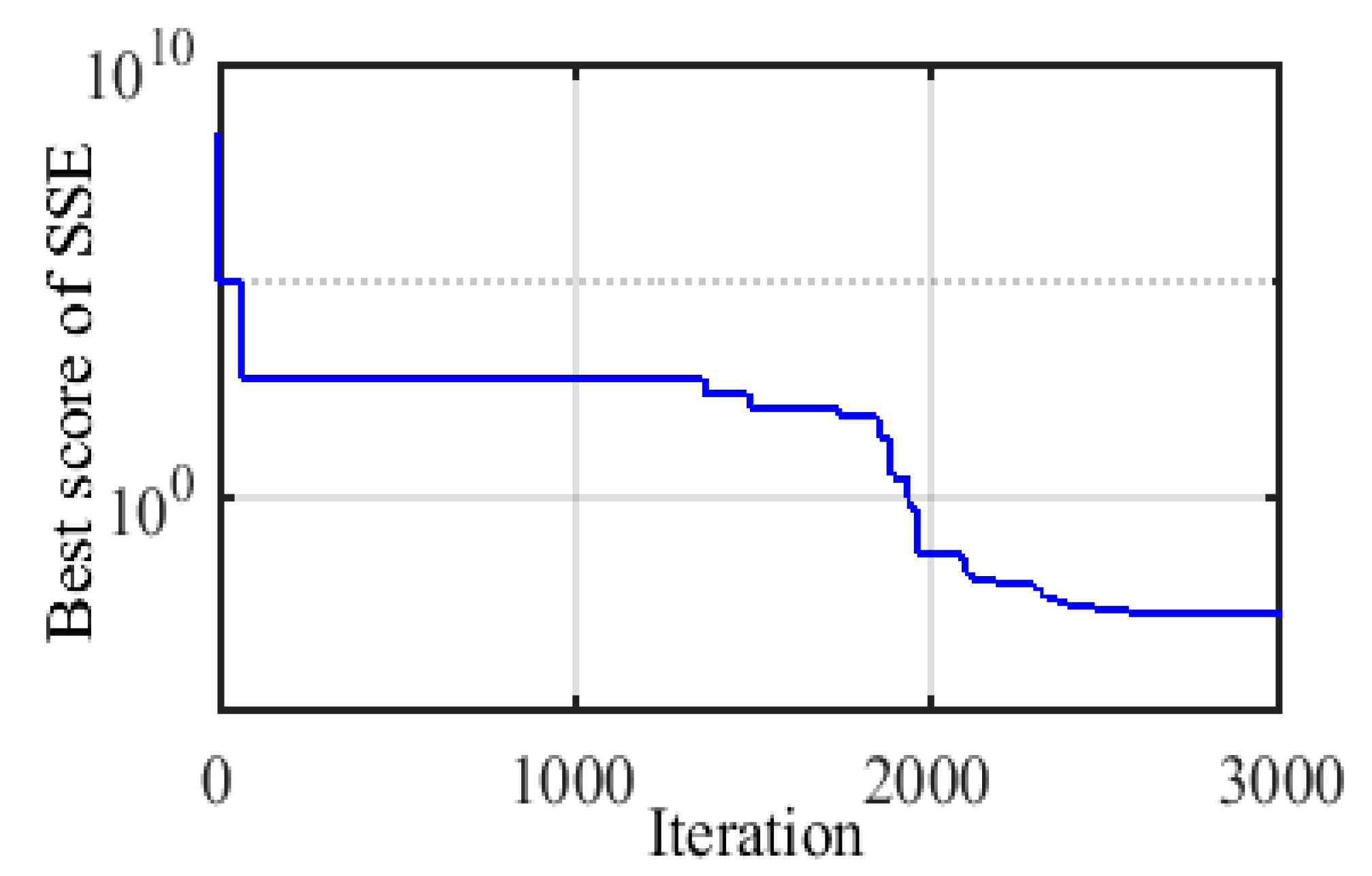
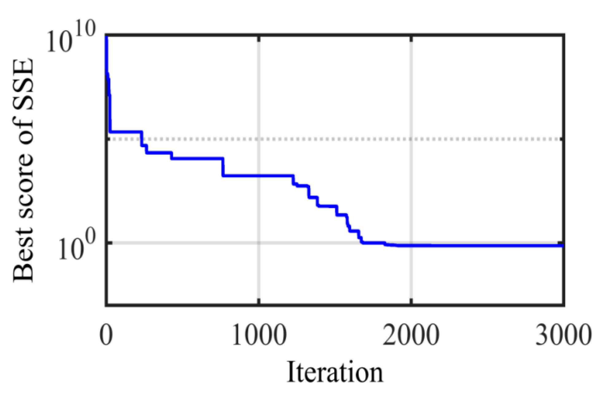
The finest estimated parameters of the PEM fuel cell model by ASO are displayed in

Table 2. Estimated parameters by ASO for SR-12 modular.

Parameter	${\mathsf{\xi }}_1$	${\mathsf{\xi }}_2$	${\mathsf{\xi }}_3$	${\mathsf{\xi }}_4$	$\mathsf{\Psi }$	${\mathbf{R}}_{\mathbf{C}}$	$\mathbf{b}$
Optimized Value	−0.9217	0.0033	0.0001	−0.0001	13.7608	0.0001	0.1497

. The convergence tendency of the SSE diagram is illustrated in Figure 4, which indicates that SSE obtained by ASO is 0.00203. MSE can be computed by (12) to result in (MSE = 0.0001015). These SSE and MSE are the smallest values compared to other challenging optimization methods, as shown in

Table 3. SR-12 modular.

Algorithm	ADE [17]	IGHS [18]	TRADE [21]	ASO
MSE	0.11885	0.1039	0.247013	0.0001015
Algorithm	GOA [25]	GWO [26]	ASO
SSE	0.0478	1.517	0.00203

.

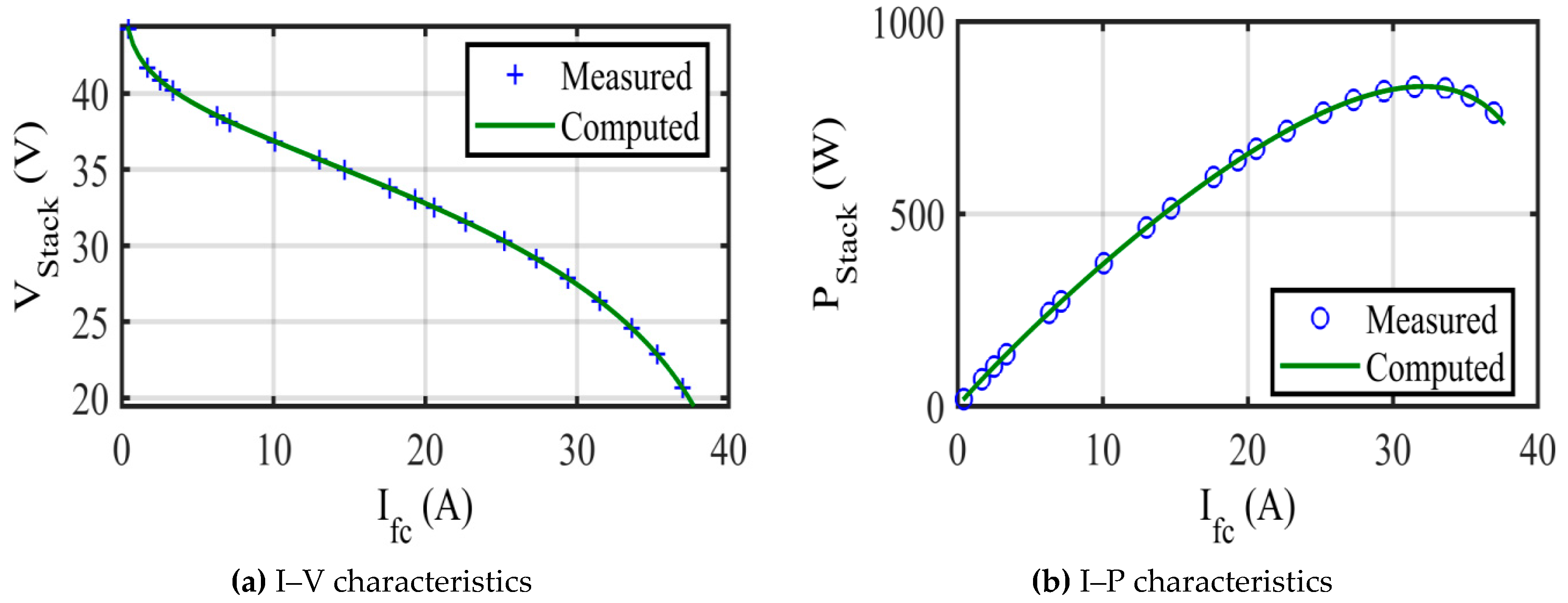
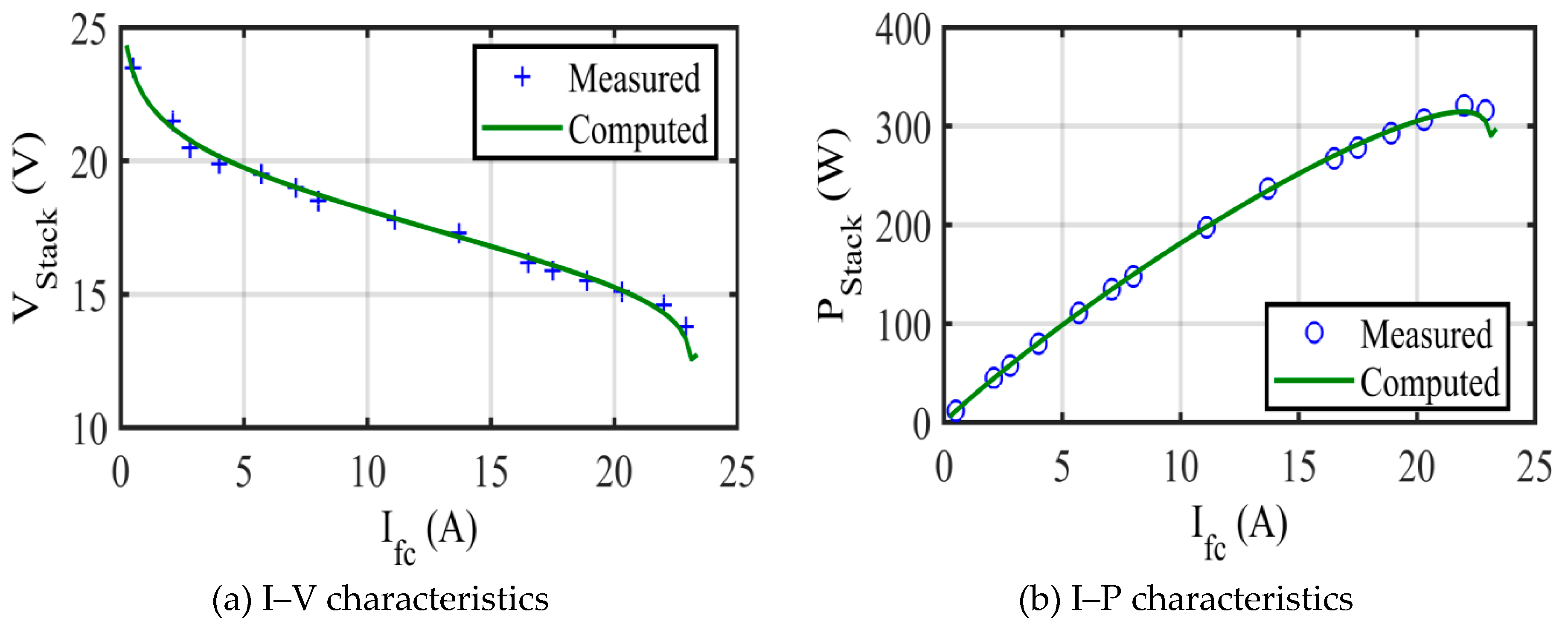
The yielded finest results for I–V characteristics of SR-12 modular PEM fuel cell that were estimated by ASO accompanying the experimentation data are displayed in Figure 5a. Closeness between the experimental voltages and computed voltages by ASO-based methodology ensures precision of the yielded optimized values of the obscure seven parameters.

The power of the SR-12 modular PEM fuel cell stack was computed using (10) and utilized to characterize the I–P relationship in Figure 5b accompanying the experimentation data. Closeness between the experimental powers and computed powers resulted due to closeness between corresponding voltages.

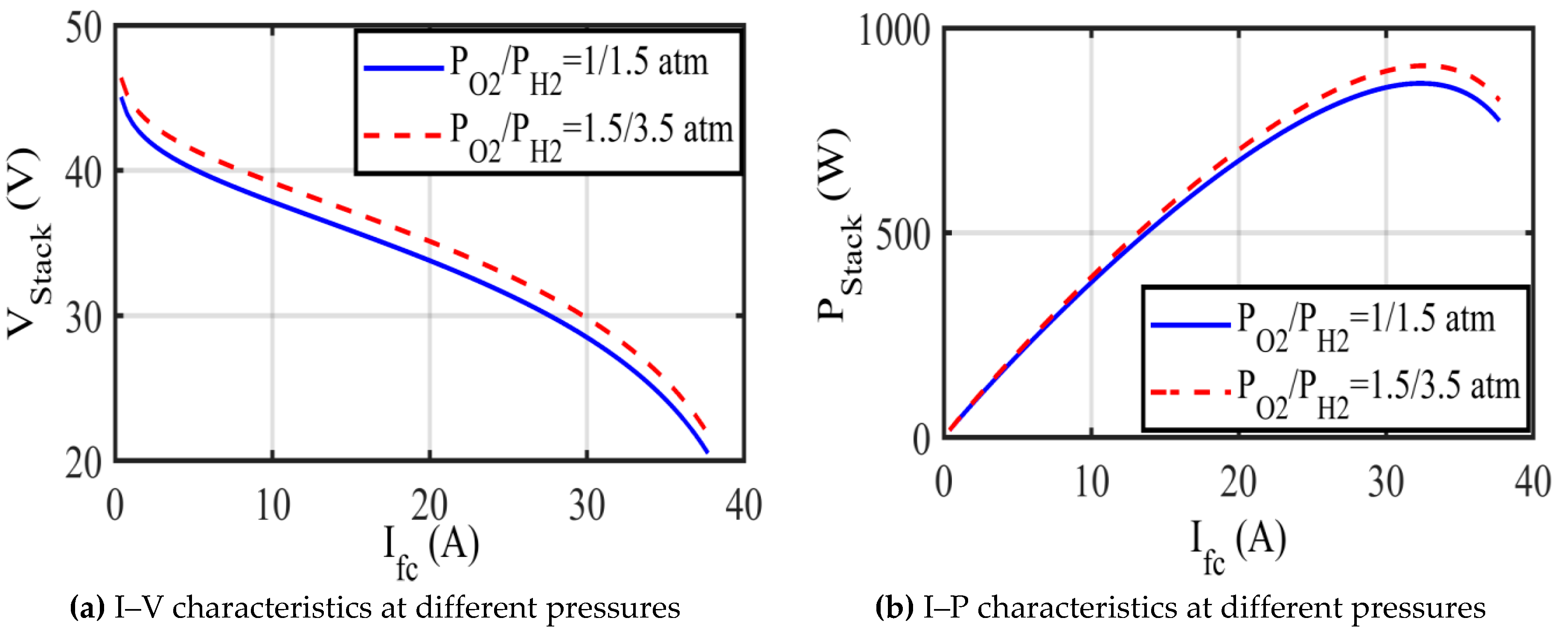
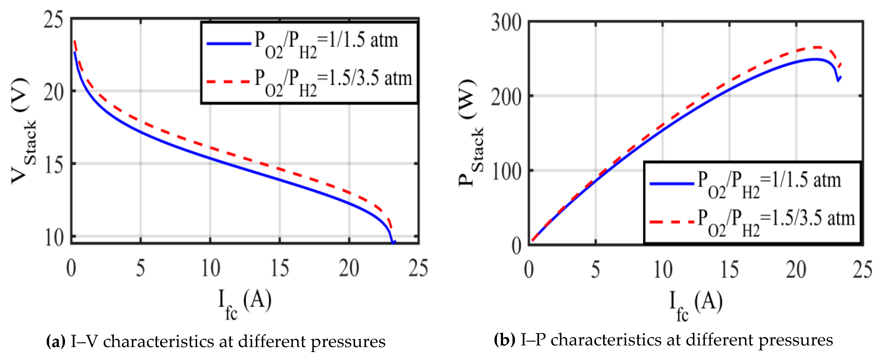
The I–V and I–P relationships of the SR-12 fuel cell stack needed to be characterized at different operating pressures and temperatures to illustrate ASO functioning at different conditions. In Figure 6, ${\mathrm{P}}_{{\mathrm{H}}_2}/{\mathrm{P}}_{{\mathrm{O}}_2}$ are 1.5/1 atm and 3.5/1.5 atm, consecutively, at a fixed temperature of 323 K. It can be noticed that increasing ${\mathrm{P}}_{{\mathrm{H}}_2}/{\mathrm{P}}_{{\mathrm{O}}_2}$ results in increasing the output voltage and power of the fuel cell stack.

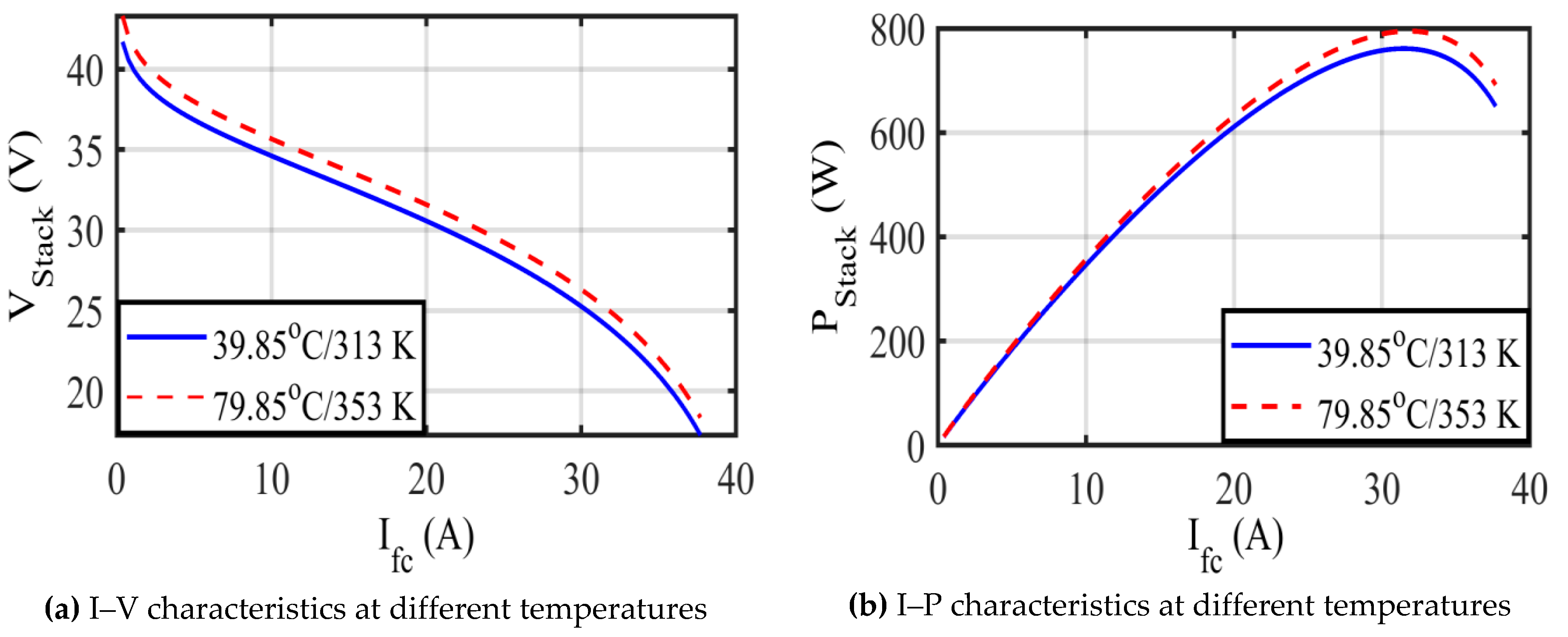
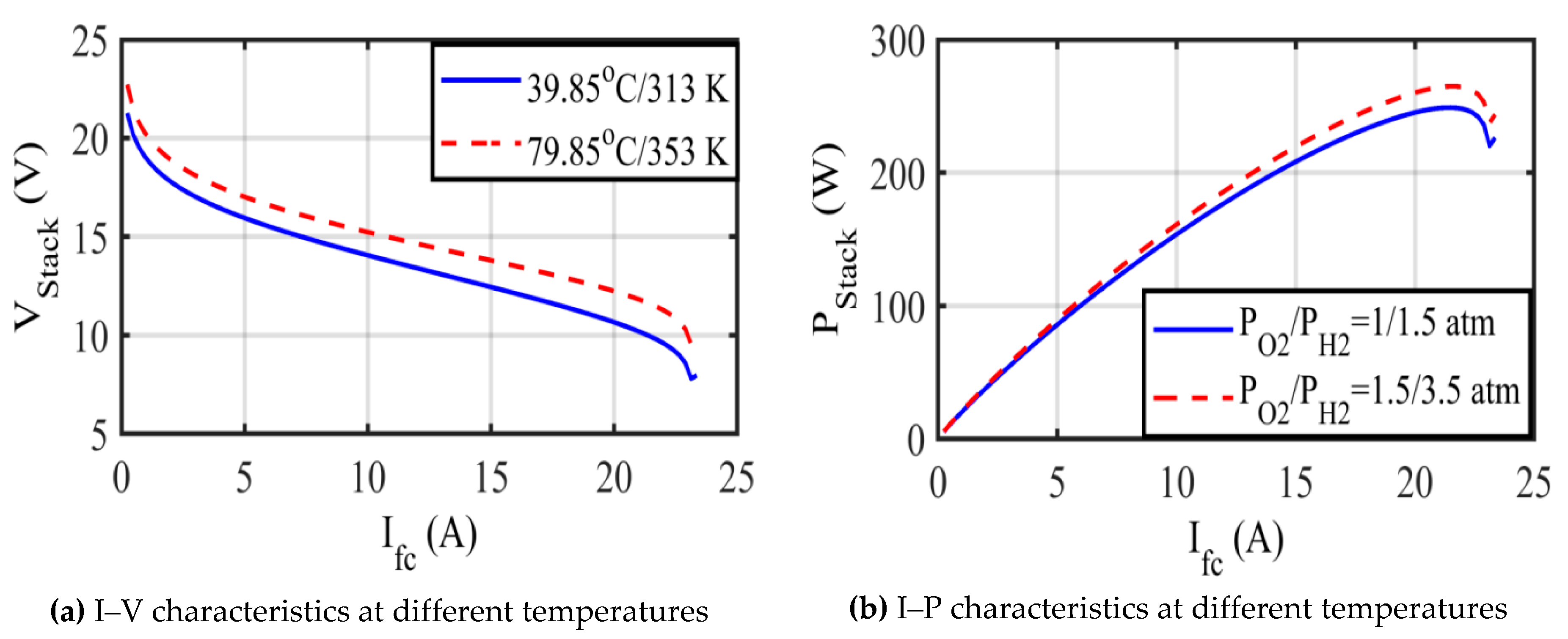
Subsequently, the influence of temperature alterations is depicted in Figure 7, where ${\mathrm{T}}_{\mathrm{fc}}$ is 313 K and 353 K, consecutively (under a fixed ${\mathrm{P}}_{{\mathrm{H}}_2}/{\mathrm{P}}_{{\mathrm{O}}_2}$ of 1/1 atm). It is clear that increasing temperature causes augmentation of the output voltage and power of the fuel cell stack.

5.2. Test Case 2

In this case, the model of the 250 W PEM fuel cell stack was tested to assure regularity of the performance of ASO. The datasheet was taken from [8,19,20,22,24,27] as follows: ${\mathrm{n}}_{\mathrm{cells}}=24$, $\mathrm{A}=27{\mathrm{cm}}^2$, $\mathrm{l}=0.178\mathrm{mm}$, ${\mathrm{J}}_{\max }=0.86\mathrm{A}/{\mathrm{cm}}^2$, ${\mathrm{T}}_{\mathrm{fc}}=338.15\mathrm{K}$, ${\mathrm{P}}_{{\mathrm{H}}_2}=1\mathrm{atm}$, and ${\mathrm{P}}_{{\mathrm{O}}_2}=1\mathrm{atm}$. Fifteen measurements in I–V characteristics of the fuel cell (M = 15) were utilized in optimization using the ASO-based proposed method.

The finest estimated parameters of the PEM fuel cell model by ASO are presented in

Table 4. Estimated parameters by the ASO for the 250 W stack.

Parameter	${\mathsf{\xi }}_1$	${\mathsf{\xi }}_2$	${\mathsf{\xi }}_3$	${\mathsf{\xi }}_4$	$\mathsf{\Psi }$	${\mathbf{R}}_{\mathbf{C}}$	$\mathbf{b}$
Optimized Value	−1.1132	0.0036	0.0001	−0.0002	22.1763	0.0001	0.0248

. The convergence leaning of SSE diagram is displayed in Figure 8, which illustrates that the SSE received from ASO is 0.7346. This SSE is the lowest value compared to those of other challenging optimization methods, as shown in

Table 5. 250 W PEM fuel cell stack.

Algorithm	ARNA-GA [8]	BBO-M [19]	STLBO [20]	HADE [22]	MVO [24]	BIPOA [27]	ASO
SSE	8.1039	7.6165	7.6266	7.9908	3.5846	7.9416	0.7346

. MSE can be computed by (12), resulting in MSE = 0.04897.

The obtained finest results for the I–V characteristics of the 250 W PEM fuel cell stack that were estimated by ASO accompanying the experimentation data are displayed in Figure 9a. Closeness between the experimental voltages and computed voltages by ASO-based methodology ensures precision of the got optimized values of the obscure seven parameters.

The power of the 250 W PEM fuel cell stack is computed using (10) and utilized to characterize the I–P relationship in Figure 9b accompanying the experimentation data. Nearness between the experimental voltages and computed voltages causes nearness between corresponding powers.

To verify ASO functioning at different conditions, the I–V and I–P relationships of the 250 W fuel cell stack needed to be characterized at different operating pressures and temperatures. In Figure 10, ${\mathrm{P}}_{{\mathrm{H}}_2}/{\mathrm{P}}_{{\mathrm{O}}_2}$ are 1.5/1.5 atm and 3/2.5 atm, consecutively, at a fixed temperature of 338 K. It can be observed that increasing ${\mathrm{P}}_{{\mathrm{H}}_2}/{\mathrm{P}}_{{\mathrm{O}}_2}$ causes an increase in the output voltage and power of the fuel cell stack.

Afterwards, the influence of the changing temperature is displayed in Figure 11, where ${\mathrm{T}}_{\mathrm{fc}}$ is 313 K and 353 K, consecutively (under a fixed ${\mathrm{P}}_{{\mathrm{H}}_2}/{\mathrm{P}}_{{\mathrm{O}}_2}$ of 1/1 atm). It is obvious that augmentation of temperature results in increasing the output voltage and power of the fuel cell stack.

Finally, performance measures using parametric tests to testify the robustness of the ASO results were made.

Table 6. ASO-adapted controlling parameters.

Factor	SR-12 Modular	250 W Stack
Best value of SSE	0.00203	0.7346
Worst value of SSE	0.00304	1.0903
Mean value of SSE	0.00251	0.9156
STD value of SSE	$2.94\times {10}^{-4}$	0.0945
Variance of SSE	$8.71\times {10}^{-8}$	0.0089
Average processing time per run (s)	25.50	20.10

summarizes the ASO executions over 100 independent runs and associated indicators in terms of Best, Worst, standard deviation (STD), Mean, and Variance of SSE values to check the robustness and consistency. It can be said here that the smaller values of STD and variance prove the robustness of the obtained results and indicate that the adapted ASO control parameters were carefully selected.

6. Conclusions

ASO-based methodology has been introduced for estimating the PEM fuel cell model parameters to assure precise modeling and simulation. The finest values of obscure parameters are generated by the ASO, for two real commercial PEM fuel cell models. The computed results of two models are compared with measured results to illustrate ASO proper functioning. Good fittings between the measured and computed voltages were evidenced through various plots and insignificant values of SSE. Comparisons between the obtained results by the ASO and other recent challenging optimization method-based results indicate the viability and qualification of the proposed ASO-based methodology. Finally, performance measures were made which reprove the good performance and robustness of the ASO-realized results. Therefore, the authors can recommend ASO as a new optimization tool for other engineering complicated problems, which really still needs further verifications.

References

- Alshehri, F.; Suarez, V.G.; Torres, J.L.R.; Perilla, A.; Van Der Meijdena, M.A.M.M. Modelling and Evaluation of PEM Hydrogen Technologies for Frequency Ancillary Services in Future Multi-Energy Sustainable Power Systems. Heliyon 2019, 5, e01396. [Google Scholar] [CrossRef]
- Satpathy, S.; Padhee, S.; Bhuyan, K.C.; Ingale, G.B. Mathematical modelling and voltage control of fuel cell. In Proceedings of the International Conference on Energy Efficient Technologies for Sustainability (ICEETS), Nagercoil, India, 7–8 April 2016. [Google Scholar] [CrossRef]
- Priya, K.; Sathishkumar, K.; Rajasekar, N. A comprehensive review on parameter estimation techniques for Proton Exchange Membrane fuel cell modelling. Renew. Sustain. Energy Rev. 2018, 93, 121–144. [Google Scholar] [CrossRef]
- Papurello, D.; Silvestri, S.; Tomasi, L.; Belcari, I.; Biasioli, F.; Santarelli, M. Biowaste for SOFCs. Energy Procedia 2016, 101, 424–431. [Google Scholar] [CrossRef]
- Santarelli, M. Carbon recovery and re-utilization (CRR) from the exhaust of a solid oxide fuel cell (SOFC): Analysis through a proof-of-concept. J. CO2 Util. 2017, 18, 206–221. [Google Scholar] [CrossRef]
- Martin, I.S.; Ursua, A.; Sanchis, P. Modelling of PEM Fuel Cell Performance: Steady-State and Dynamic Experimental Validation. Energies 2014, 7, 670–700. [Google Scholar] [CrossRef] [Green Version]
- El-Fergany, A.A. Extracting optimal parameters of PEM fuel cells using salp swarm optimizer. Renew. Energy 2018, 119, 641–648. [Google Scholar] [CrossRef]
- Zhang, L.; Wanga, N. An adaptive RNA genetic algorithm for modeling of proton exchange membrane fuel cells. Int. J. Hydrogen Energy 2013, 38, 219–228. [Google Scholar] [CrossRef]
- Tafaoli-Masoule, M.; Bahrami, A.; Elsayed, E.M. Optimum design parameters and operating condition for maximum power of a direct methanol fuel cell using analytical model and genetic algorithm. Energy 2014, 70, 643–652. [Google Scholar] [CrossRef]
- Priya, K.; Babu, T.; Balasubramanian, K.; Kumar, K.; Rajaseka, N. A novel approach for fuel cell parameter estimation using simple Genetic Algorithm. Sustain. Energy Technol. Assess. 2015, 12, 46–52. [Google Scholar] [CrossRef]
- Rajaseka, N.; Jacob, B.; Balasubramanian, K.; Priya, K.; Sangeetha, K.; Babu, T.S. Comparative study of PEM fuel cell parameter extraction using Genetic Algorithm. Ain Shams Eng. J. 2015, 6, 1187–1194. [Google Scholar] [CrossRef] [Green Version]
- Salim, R.I.; Noura, H.; Fardoun, A. A Parameter identification approach of a PEM fuel cell stack using particle swarm optimization. In Proceedings of the ASME 2013 11th International. Conference on Fuel Cell Science, Engineering and Technolog, Minneapolis, MA, USA, 14–19 July 2013. [Google Scholar] [CrossRef]
- Chang, K.Y. The optimal design for PEMFC modeling based on Taguchi method and genetic algorithm neural networks. Int. J. Hydrogen Energy 2011, 36, 13683–13694. [Google Scholar] [CrossRef]
- Askarzadeh, A.; Rezazadeh, A. A new heuristic optimization algorithm for modeling of proton exchange membrane fuel cell: Bird mating optimizer. Int. J. Energy Res. 2013, 37, 1196–1204. [Google Scholar] [CrossRef]
- Dai, C.; Chen, W.; Cheng, Z.; Li, Q.; Jiang, Z.; Jia, J. Seeker optimization algorithm for global optimization: A case study on optimal modelling of proton exchange membrane fuel cell. Int. J. Electr. Power Energy Syst. 2011, 33, 369–376. [Google Scholar] [CrossRef]
- Guarnieri, M.; Negro, E.; Noto, V.; Alotto, P. A selective hybrid stochastic strategy for fuel-cell multi-parameter identification. J. Power Sources 2016, 332, 249–264. [Google Scholar] [CrossRef]
- Cheng, J.; Zhang, G. Parameter fitting of PEMFC models based on adaptive differential evolution. Int. J. Electr. Power Energy Syst. 2014, 62, 189–198. [Google Scholar] [CrossRef]
- Askarzadeh, A.; Rezazadeh, A. An innovative global harmony search algorithm for parameter identification of a PEM fuel cell model. IEEE Trans. Ind. Electron. 2012, 59, 3473–3480. [Google Scholar] [CrossRef]
- Niu, Q.; Zhang, L.; Li, K. A biogeography-based optimization algorithm with mutation strategies for model parameter estimation of solar and fuel cells. Energy Convers. Manag. 2014, 86, 1173–1185. [Google Scholar] [CrossRef]
- Niu, Q.; Zhang, H.; Li, K. An improved TLBO with elite strategy for parameters identification of PEM fuel cell and solar cell models. Int. J. Hydrogen Energy 2014, 39, 3837–3854. [Google Scholar] [CrossRef]
- Gong, W.; Yan, X.; Xiaobo, L.; Cai, Z. Parameter extraction of different fuel cell models with transferred adaptive differential evolution. Energy 2015, 86, 139–151. [Google Scholar] [CrossRef]
- Sun, Z.; Wang, N.; Bi, Y.; Srinivasan, D. Parameter identification of PEMFC model based on hybrid adaptive differential evolution algorithm. Energy 2015, 90, 1334–1341. [Google Scholar] [CrossRef]
- Sankar, K.; Jana, A.K. Dynamics and estimator-based nonlinear control of a PEM fuel cell. IEEE Trans. Control Syst. Technol. 2018, 26, 1124–1131. [Google Scholar] [CrossRef]
- Fathy, A.; Rezk, H. Multi-verse optimizer for identifying the optimal parameters of PEMFC model. Energy 2018, 143, 634–644. [Google Scholar] [CrossRef]
- El-Fergany, A.A. Electrical characterisation of proton exchange membrane fuel cells stack using grasshopper optimiser. IET Renew. Power Gener. 2018, 12, 9–17. [Google Scholar] [CrossRef]
- Ali, M.; El-Hameed, M.A.; Farahat, M.A. Effective parameters’ identification for polymer electrolyte membrane fuel cell models using grey wolf optimizer. Renew. Energy 2017, 111, 455–462. [Google Scholar] [CrossRef]
- Yang, S.; Wang, N. A novel P systems based optimization algorithm for parameter estimation of proton exchange membrane fuel cell model. Int. J. Hydrogen Energy 2012, 37, 8465–8476. [Google Scholar] [CrossRef]
- Zhao, W.; Wanga, L.; Zhang, Z. Atom search optimization and its application to solve a hydrogeologic parameter estimation problem. Knowl.-Based Syst. 2019, 163, 283–304. [Google Scholar] [CrossRef]
- Zhao, W.; Wanga, L. A novel atom search optimization for dispersion coefficient estimation in groundwater. Future Gener. Comput. Syst. 2019, 91, 601–610. [Google Scholar] [CrossRef]
- Goldstein, H.; Poole, C.P.; Safko, J.L. Classical Mechanics, 3rd ed.; Addison Wesley: Boston, MA, USA, 2001. [Google Scholar]
Figure 1.
Atoms force against spacing between them [29].
Figure 2.
Function F′ against η [28].
Figure 3.
Forces in an atom arrangement through when K = 4 [29].
Figure 4.
Sum of the squared error (SSE) convergence for SR-12 modular.
Figure 5.
Characteristics of SR-12.
Figure 6.
Characteristics of SR-12 at different pressures.
Figure 7.
Characteristics of SR-12 at different temperatures.
Figure 8.
SSE convergence for the 250 W stack.
Figure 9.
Characteristics of the 250 W stack.
Figure 10.
Characteristics of the 250 W stack at different pressures.
Figure 11.
Characteristics of the 250 W stack at different temperatures.