Using Text Mining to Estimate Schedule Delay Risk of 13 Offshore Oil and Gas EPC Case Studies During the Bidding Process


1
Hyundai Heavy Industries (HHI), Project Management Team, 400 Bangeojinsunhwan-doro, Dong-gu, Ulsan 44114, Korea
2
Graduate School of Engineering Mastership (GEM), Pohang University of Science and Technology (POSTECH), 77 Cheongam-Ro, Nam-Ku, Pohang 37673, Korea
3
Department of Industrial and Management Engineering, Pohang University of Science and Technology (POSTECH), 77 Cheongam-Ro, Nam-Ku, Pohang 37673, Korea
*
Author to whom correspondence should be addressed.
Energies 2019, 12(10), 1956; https://doi.org/10.3390/en12101956
Submission received: 21 April 2019
/
Revised: 9 May 2019
/
Accepted: 17 May 2019
/
Published: 22 May 2019
(This article belongs to the Special Issue Applications of Engineering Digitalization and Construction IT for Energy Projects)
Abstract
:Korean offshore oil and gas (O&G) mega project contractors have recently suffered massive deficits due to the challenges and risks inherent to the offshore engineering, procurement, and construction (EPC) of megaprojects. This has resulted in frequent prolonged projects, schedule delay, and consequently significant cost overruns. Existing literature has identified one of the major causes of project delays to be the lack of adequate tools or techniques to diagnose the appropriateness and sufficiency of the contract deadline proposed by project owners prior to signing the contract in the bid. As such, this paper seeks to propose appropriate or correct project durations using the research methodology of text mining for bid documents. With the emergence of ‘big data’ research, text mining has become an acceptable research strategy, having already been utilized in various industries including medicine, legal, and securities. In this study the scope of work (SOW), as a main part of EPC contracts is analyzed using text mining processes in a sequence of pre-processing, structuring, and normalizing. Lessons learned, collected from 13 executed off shore EPC projects, are then used to reinforce the findings from said process. For this study, critical terms (CT), representing the root of past problems, are selected from the reports of lessons learned. The occurrence of the CT in the SOW are then counted and converted to a schedule delay risk index (SDRI) for the sample projects. The measured SDRI of each sample project are then correlated to the project’s actual schedule delay via regression analysis. The resultant regression model is entitled the schedule delay estimate model (SDEM) for this paper based on the case studies. Finally, the developed SDEM’s accuracy is validated through its use to predict schedule delays on recently executed projects with the findings being compared with actual schedule performance. This study found the relationship between the SDRI, frequency of CTs in the SOW, and delays to be represented by the regression formula. Through assessing its performance with respect to the 13th project, said formula was found to have an accuracy of 81%. As can be seen, this study found that more CTs in the SOW leads to a higher tendency for a schedule delay. Therefore, a higher project SDRI implies that there are more issues on projects which required more time to resolve them. While the low number of projects used to develop the model reduces its generalizability, the text mining research methodology used to quantitatively estimate project schedule delay can be generalized and applied to other industries where contractual documents and information regarding lessons learned are available.
1. Introduction
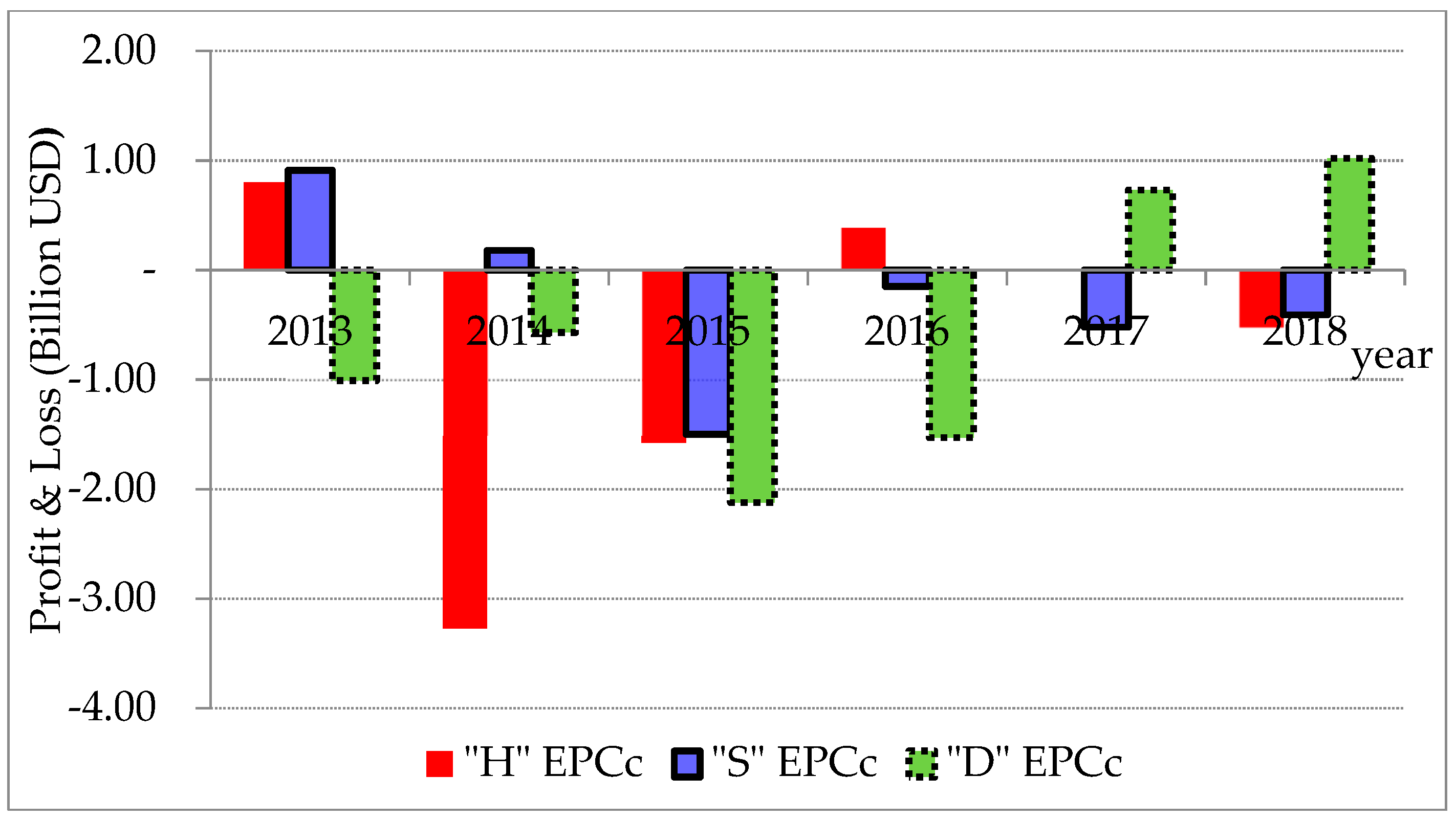
According to the Korea Energy Economics Institute [1], offshore projects have been selected as a solution to end the stagnation of the shipbuilding industry caused by the poor business performance of the shipping industry since the global economic crisis in 2008. However, these projects have recorded massive deficits equating to a major restructuring of the domestic shipbuilding industry as a whole. In the 2010s, the top three domestic shipbuilders thus began to execute engineering, procurement, and construction (EPC) lump sum turnkey projects. In this contract, the EPC contractor undertakes all the risks and responsibilities of the contract at the time of award. These contracts can result in high profitability for all parties if the process is adhered to as planned and if there are no special risks. However, this is not the reality as, from 2013, there have been consistent losses made in EPC projects, as shown in Figure 1. As can be seen (i.e., according to the publically listed information in Korea Financial Supervisory Service), three major Korean offshore EPC contractors (companies H, S, and D) have recorded total profit loss of approximately USD 10 billion during the period between 2013 and 2015, with little lessor deficits being experienced in 2016 and 2017.
The Korea Energy Economics Institute [2] has identified the cause of these large-scale offshore mega EPC project deficits as follows: (1) lack of contractor’s capabilities for the design and engineering of offshore EPC projects, (2) the highly customized and non-standardized characteristics of offshore projects, (3) over-competition among domestic shipbuilders to preempt the offshore O&G market resulting in low price bids, and (4) a general lack of recognition with respect to the significance of EPC contracts and professional experience, or a lack of achievable project scheduling. Most of these identified causes of profit loss deficit equate to significant project schedule delays. According to Johansen et al. [3], project schedule delay is one of the main causes of project cost increases. Thus, increasing schedule efficiencies to minimize delays is an effective measure to reduce the level of deficit. A study of major offshore O&G EPC project schedule delays conducted across 45 worldwide floating production storage and offloading (FPSO), conversion of oil tankers, between 2008 and 2012, found project delays on 30 of the 45 FPSO units. An in-depth analysis of the nine of those FPSOs revealed project schedule delays of more than 12 years in accumulation (about 16 months per project) and cost overruns of 38% as shown in Table 1 [4].
Furthermore, from subject matter expert (SME) interviews, the most impactful causes of domestic offshore EPC contractor schedule delays in Korea were unreasonably short project durations as requested by the owners being accepted due to high competition and a lack of tools to quantitatively verify owner requested project duration prior to signing the contract in the bid process. Thus, this study aims to develop a model that can diagnose the risk of O&G megaproject schedule delay prior to signing the contract. The authors chose to use the Korean EPC contractor’s experience to represent the industry as a whole as their experience is of significance to the O&G industry. Key Korean EPC contractors have played a major role in the execution of O&G mega EPC projects in the global market over last two decades. For example, at the market peak (i.e., 2010–2015), the largest Korean EPC contractors performed about USD 10 billion dollars’ worth of O&G offshore EPC contracts per year with the average project size being 1.5–2.5 billion USD. According to some statistics by Korean Energy Economics Institute [2], the major three offshore EPC contractor at the peak was about 30–40 billion USD, which covered about 60%–70% of global market contract.
The proposed schedule delay estimate model (SDEM) is expected to aid EPC contractor management in quantifying possible construction delays prior to accepting contractual schedule durations. Said model has been developed by using text mining to analyze and categorize significant schedule indicators as identified in collected contract documents, specifically the scope of work (SOW), and as-built lessons learned reports. Due to the diversity of contractor responsibilities, EPC contracts consists of extremely complicated components in comparison to design-bid-build where the contractor’s main responsibility is to only construct a facility based off a completed design provided by the project owner. There is no standard form of contract for EPC Projects, although the International Federation of Consulting Engineers (FIDIC) Silverbook is often used by many onshore EPC owners in practice, especially the owners of O&G. Mega-corporations such as the national oil company Aramco of Saudi Arabia, or PetroBras in Brazil, and international oil companies such as Exxon Mobil and Shell use their own contract templates. This equates to a general lack of contract standardization in EPC contracts which contain a huge volume of owners’ legal, commercial, and technical requirements. While the contract documents vary based on the project, typically EPC Contracts consists of: (1) condition of contract as the main body of the agreement to cover mainly legal and commercial requirement and (2) attachments in the form of appendix, exhibits, annex and schedule; including scope of work as the main part, specifications, and owner provided drawings. A typical list of table of contents for condition of contract and exhibit, including SOW topics is illustrated in Appendix A. Thus, the resultant model, through the use of text mining and executed SOWs, is expected to be very useful for contractors to quickly and efficiently assess the schedule delay risk index (SDRI) of complex EPC O&G contract documents within the short allowable bidding time, typically about 2–3 months for offshore EPC projects.
2. Literature Review
This publication largely builds upon existing literature within the categories of EPC megaproject duration estimation and text mining. While not an academic publication, the Project Management Institute (PMI) [5] provides the industry-accepted scheduling estimation practices across all construction sectors. The typical schedule activity duration estimation techniques used on offshore O&G projects include analogous, parametric, and three-point estimation. The analogous method estimates the duration of a new project based on the historical data of similar projects. It is the least accurate technique but is quick and is often used on O&G EPC projects due to the accelerated bid response time requirements. Parametric estimation is more accurate, using historical activity data and project parameters and characteristics to achieve project duration (For example, historically company A installs an average of 20 widgets/hour in location ‘x’. For a project near location x and a scope of 100 widgets, said company would estimate 5 h). This method can be highly accurate but is both demanding in terms of resources and time, making it difficult to perform on EPC offshore O&G projects which have thousands of activities and short bidding periods. Finally, three-point estimating incorporates each activity’s risk by defining the optimistic, most likely, and pessimistic durations to create a probable distribution of schedule durations. Once again, this is a useful technique, especially early in the project when there are many unknowns, but improbable on EPC offshore O&G projects.
Concerning research within scheduling and scheduling risk management, Rawash et al. [6] assess the various risks which impact EPC schedule performance from project conception to completion. They assess the standard conditions of contracts through PMI’s pre-defined risk management process to develop a model which assists contract administrators to diminish time and effort in developing, reviewing, and understanding contractual agreements. The result is a more efficient and collaborative contract environment which includes a lessons learned database to ensure effective contractual agreement evolution as necessary. Yeo and Ning [7] focus on optimizing procurement management to minimize delays, proposing an enhanced framework which combines the concepts of supply chain management and critical chain project management. Said framework cultural, process and technological improvements, giving special to a systems approach of buffer management as a mechanism to improve the management of risk in procurement. Bevilacqua et al. [8] also utilize critical chain project management to propose a method of prioritizing work packages to minimize risks related to refinery plant accidents. Öztaş and Ökmen [9] aiding contractors in assessing risks from the contract during the bidding stages present common risks that exist in the typical design-build contract to propose a schedule and cost risk analysis model. Their study was performed through a literature review and was focused on fixed-price commercial, industrial, and governmental vertical construction. Bali and Apte [10] also identified potential risks in an EPC contract, performing a case study on the construction of a raw water intake system for a thermal power plant. They classified the risks into 19 categories, identifying the categories of risk inherent in each work breakdown structure activity.
Through an extensive nationwide survey of Jordanian construction stakeholders, one study identified the most common causes of construction delay to be owner interference, inadequate contractor experience, financing and payments, labor productivity, slow decision making, improper planning, and subcontractors [11]. In less developed nations, construction delays were found to be caused by corruption, unavailability of utilities at site, inflation, lack of quality materials, delay in design documents, slow delivery of materials, delayed owner approvals, poor site management, late payments, and ineffective project planning [12,13,14]. Chang [15] assess the reasons for cost and schedule increases specifically in the design portion, identifying owner’s change requests, omissions, poor schedule estimation, and general failures; consultants lack of ability and/or omissions; and general growing needs, stakeholders and changing of governing specifications as the largest impacting factors. Overall, it has been estimated that 70% of projects experience an average schedule overrun between 10% and 30% due to these issues [16] with larger projects, such as offshore EPC O&G megaprojects, more likely to experience the higher end of that range [17]. Olawale and Sun present 90 mitigating measures for design, general risk, schedule estimation, complexity, and subcontract management to prevent, predict, and/or correct the sources of overruns [18]. However, no amount of mitigation will completely remove the overruns, and overruns which often result in a plethora of contractor claims. In response to this, Iyer et al. [19] propose a rule-based expert system to assist contract administrators in assessing claims validity from a contractual stand-point to avoid lengthy and expensive litigations.
While there exist a multitude of studies modelling construction schedules, research on estimating schedules and predicting the potential delays for O&G project construction related to automated modelling are few. A detailed engineering completion rating index system model was developed and implemented to assist offshore EPC contractors for optimizing fabrication and construction work schedule with minimizing possibility of repetition of works [20,21]. Jo et al. [22] developed a methodology of piping construction delay prevention to improve material procurement management and avoid shortage of piping materials and to minimize delays, by using the critical chain project management. These studies contributed to reducing schedule delays and potential liquidated damages, also called DLD (delay liquidated damages).
EPC offshore O&G contractors are often forced to use the quick yet inaccurate analogous estimation method as they have very little time to accurately estimate schedule durations during the bidding period. While this paper is focused on O&G projects, this is an industry-wide issue. Many publications have analyzed big data sets to create models that estimate construction processes, including schedule duration, and require very little time yet produce accurate results in an attempt to solve this problem. One method of big data analysis is text mining. Text mining is not a recent technology but has seen a growth in its use as the analysis of big data sets has grown popular. The process is defined in much greater detail in Section 3.2.2 below but is generally defined by the following five steps: importing documentation, cleaning data prior to assessment (pre-processing), prepping data for assessment (structuring), normalizing, and analyzing [23]. In short, text mining extracts information from documents through the natural language processing [24] and converts said text to quantitative patterns, trends, and/or relationships for further assessment [25]. It is an excellent strategy for assessing the construction industry because most of the information is stored in text form rather than quantitatively [26]. Text mining is different from general data mining [27] as it quantifies or structures existing qualitative or unstructured data. In comparison, general data mining performs analyses on data that is already structured and/or quantified [28]. The following paragraphs describe existing research which has used text mining to improve project processes.
When attempting to use new technologies, as is often the case on O& G projects, firms are required to review existing patents to assess how to approach new business opportunities (ex. create a new technology or buy existing one). Wang et al. [29] used text mining and word sense disambiguation to develop a tool which simplifies legal jargon and reduces the number of searchable dimensions to create a patent map that can be easily understood by users to assess relevant patents. Fan and Li [30] collected text data from site accidents and developed an alternative dispute resolution document for the resulting stakeholders’ disputes. To develop this tool, they formed a vector space model, assigning a weight to each critical term in order to find a high rank case based on a similarity measure. The similarity measure is based on the distance between the feature vectors, so it was used as a measure of the relative rank order or likelihood, intensity, and type of dispute between cases. Shen et al. [31] presented a process which combines case-based reasoning and text mining to compare the efficacy of similar green building designs in an attempt to optimize the sustainability of future green building design. Arif-Uz-Zaman et al. [32] built a keyword dictionary from work orders and downtime reports to analyze the failure time of industrial production plants. Lee and Yi [33] conducted a study to predict the risk involved in the bidding process of a construction project. They analyzed the bidding documents to assess the most important or risk-intense documentation. Bidding risk prediction modeling was done by text mining pre-bid clarification information, with the pre-bid request for information documents found as the most impactful to risk prediction. They found their text mining model to improve project risk assessment accuracy by approximately 20 percent compared to traditional quantitative data models.
While the above are relevant, this paper most significantly builds off of Williams and Gong’s [34] project description text mining, Marzouk et al.’s [35] contractual text mining, Choudhary et al.’s [36] use of lessons learned to improve processes, and Pinto et al. [37] and Lotfian et al.’s [38] models which aid optimization negotiations. Williams and Gong [34] conducted a study assessing the text contained within construction projects’ descriptions to predict expected cost performance. In their assessment, they defined the cost performance as under, near, and high and assessed the description text of each project. They found a correlation between critical terms used in the project description and the cost performance. In addition, they investigated the data using quantitative project characteristics and found the text mining analysis to be more accurate. Marzouk et al. [35] developed a dynamic text analytical model for contract and correspondence, a form of text mining, to identify critical contractual (including SOW) terms related to the most impactful contractors’ obligations. Choudhary et al. [36] attempted to discover trends, patterns, and associations among lessons by applying text mining lessons learned as a way to prevent recurring problems, improve processes, and improve customer relationships. Finally, Loftian et al. [38] and Pinto et al. [37] developed models which aid contractors to estimate realistic schedules during contract assessment. Loftian et al. [38] used the Hypertext system to store schedule risks experienced by historical projects in the form of text, graphics, and pictures. Said stored information is then processed and analyzed similar to text-mining. The final model aids contractors through understanding and scheduling for uncertainty. Alternatively, Pinto et al. [37] used artificial intelligence to apply game theory on bilateral contract negotiations in the energy sector. They contended that the resultant model would aid energy EPC contractor decision-makers to overcome their existing knowledge gap of effective and realistic decision support, similar to the O&G sector.
This publication builds off of these findings by using text mining to collect data pertaining to the project description [34], SOW [35], and lessons learned [36] to optimize O&G EPC contractor’s ability to successfully execute contract negotiations [37,38] by effectively assessing project schedules during accelerated bid periods. The novelty of this paper is in combining the existing literature’s text mining analyses approaches to aid O&G EPC contractor decision makers during bid assessment, proposal development, and contract negotiations. Furthermore, this study advances the general body of knowledge concerning text mining. While the adoption of big data analysis and text mining technology has seen significant potential in multiple sectors, within the construction industry is in its infancy. Through a rigorous research methodology and model validation, it is expected that the findings of this study will potentially assist EPC O&G contractor decision-makers to effectively assess whether or not to participate in bidding selected projects and, if they chose to bid, mitigate schedule delay risks revealed through the SDEM prior to contract negotiation with project owners.
3. Research Methodology
The objective of this research is to develop a tool which supports EPC O&G contractors to effectively assess schedule durations and potential risk factors during the accelerated bidding process. To do this, the authors have developed a schedule delay estimate model (SDEM) to predict project schedule performance. Said tool includes the use of text mining to identify of critical terms (CT) extracted from reports of lessons learned, organized into a schedule delay risk index (SDRI), from lessons learned and the contractor’s contractual SOW documents. To ensure applicability to schedule assessment, the authors then correlated the calculated SDRI with schedule delays from sample projects for a resultant quick and accurate predictive model. The scope of this study is limited to fixed platform and floater offshore O&G EPC projects. Other types of offshore structures and subsea structures are excluded in this study. In addition, duration of schedule delays found from sample projects and used for statistical analysis for this study is only based between effective date (i.e., contractual start for EPC projects) and sail-away date (i.e., substantial completion) from the offshore EPC contractor’s shipyard of each sample project and, therefore, duration of project activities performed offshore such as hookup is not considered in schedule performance. The lessons learned information used to survey SMEs and identify CTs are those developed from issues incurred from contractor’s yard. Finally, non-SOW contract documents such as conditions of contract, exhibits and annex are not considered for this study. The research methodology applied to develop SDEM is listed as follows, depicted in Figure 2, and explained in detail in the following subsections (RS is Research Step).
- RS 1.
- Data collection: collect lessons learned and SOW to be used for analysis
- RS 2.
- Data processing: select CTs from lessons learned by a way of expert judgment and find the normalized frequencies of the texts shown on SOW by a way of text mining
- RS 3.
- SDRI scoring: calculate SDRI by a way of mapping the selected CTs with normalized frequencies
- RS 4.
- SDEM development: build SDEM by correlating the assessed SDRI with actual schedule delay incurred from twelve sample projects
- RS 5.
- SDEM verification: verify model accuracy with a case study
3.1. Research Step 1, Data Collection
The model is developed based on lessons learned and SOW data collected from 13 offshore O&G projects that have been carried out by an offshore EPC contractor in South Korea between 2008–2018. These 13 projects were chosen out of the 18 offshore EPC projects this company had performed during this time based on their availability of data. The remaining 5 were unusable due to limitations of data access such as electronic version of contract documents (especially SOW) and availability of Lesson learned reports (i.e., CT). The 13 sample projects selected represent typical EPC contracts performed by one of the largest worldwide offshore EPC contractors. Each project’s size, characteristics, owners’ requirements are more or less similar from a practical point of view.
Said offshore EPC contractor, similar to other major onshore and offshore EPC contractors, maintains a lessons learned report system, prepared by major project participants after substantial completion or the sail away date. Collected documentation is stored on their Enterprise Resource Planning (ERP) system to capture pros and cons of project executions derived from the feedback of engineering and construction disciplines. All 13 projects provided a varying number of lessons learned, with the authors reviewing those specifically associated with potential impact on project schedule durations. While lessons learned include elements that have both positively and negatively influenced projects, this study collected only negative factors as its focus is to identify and mitigating schedule risks [36]. The lessons learned data was analyzed to identify potential CTs, which were validated through SME interviews. The obtained CTs were then used for schedule delay risk index (SDRI) scoring, by ensuring that the final model effectively incorporates factors that had potentially impacted on project schedule performance, which will be defined and further explained in Section 3.3.
The authors also assessed the SOW documents as it is arguably the most important contractual document, defining the EPC contractor’s working scopes and responsibilities. Furthermore, the development of the project schedule is mainly driven by the data included in the SOW. As such, analyzing the SOW provides the greatest insight into schedule factors. Table 2 shows the project type, sail-away date planned and actual dates, actual schedule delay (SD), number of pages of the document in SOW, count number of texts, word count, and the ratio of word count to count number of texts for each sample project. The text number and text frequency (word count) specified in Table 2 are counted in raw data format without preprocessing and includes objects such as numbers and annotations. The ranges of SOW length are from 36 pages up to 408 pages depending on the project. As can be seen, the number of texts increase proportionally to the number of pages. The total number of pages of SOW used in analysis was 1984 with 373 texts on each page on average. Also, one text appeared at a frequency ranging from 4.6 up to 9.5 while the overall average frequency number among all texts was 7.1. Throughout the 13 projects, 12 projects (A through L) were utilized in SDEM prediction through regression analysis with Project M being used to validate the estimated SDEM. This is discussed in more detail in Section 3.5.
3.2. Research Step 2, Data Processing
As shown in Figure 2, there are two parallel tasks occurring in RS 2, the identification of CTs through SME interviews and the text mining of the SOW.
3.2.1. Selection of Critical Terms from Lessons Learned Reports
An exhaustive list, as a draft version, of CT candidates were initially selected lessons learned reports for the 13 case study project by the authors based on related literature review and their own professional experiences (about 40 years in total) in academia and practice for EPC project management, especially contract and claims management. The draft CT list was presented and given to about eight SMEs for check and verification. As can be seen in Table 3, the SMEs they had 77 years of experience amongst them all with three and two individuals having the PMI Project Management and Risk Management Professional certifications, respectively. The authors performed face-to-face interviews with the SMEs, discussing the said CT draft list and requesting that they remove texts that were not considered as CTs and supplement texts that were not included in the original list. The resultant list through the SMEs’ check and interview included 307 CTs in total. 282 of the CTs shown in Appendix B are text that were verified to be in at least one project’s SOW and contribute to SDRI scoring step as defined below. The other 25 CTs shown in Appendix C are those that did not appear in any SOW and were therefore not included in this process of SDRI scoring step.
For the project scoring, discussed in Section 3.3, the authors excluded non-CT as only the CT are scored in the development the SDRI. To ensure the CTs generated through the lessons learned reports and associated SME interviews were appropriate, the authors reviewed project text data to see how many CTs were present in each project. 282 out of 307 identified CTs were found to appear in at least one SOW among 13 of the sample projects.
3.2.2. Text Mining of SOWs
Concurrently, the authors were assessing the SOWs by a way of the text mining process. Figure 3, below, shows the procedure for performing text mining as tailored for this study. The process can be divided into five stages: (1) import analysis data converting it into text corpus; (2) pre-processing work of the text corpus by eliminating stopwords, numbers, and symbols, and eliminating words appearing more than 300 times throughout the whole documents; (3) structure the data to a vector space model to allow for a quantified assessment; (4) normalizing the text frequency scoring across project SOWs; and (5) assessing the result. This process is shown graphically in Figure 3, with steps one through four being explained in greater detail in the subsections below and step five being included in Section 3.3 to Section 3.5.
For this study, the authors used R programming [40] version 3.4.3, an open source platform, for text data importing, pre-processing, and structuring process and the SDEM regression analysis. Microsoft Excel 2010 was used for the normalizing process and SDRI assessment.
Stage 1: Importing Data
The first step in text mining is to simply collect and import the data into a selected programming tool. The authors input the 12 projects, A through M, near-total 730,000-word count from 1984 SOW pages into the R program programming tool. The text documents are stored in said software in the form of bag-of-words [39], to go through pre-processing steps as defined below. The bag-of-words model is a simplifying representation used in which a sentence in SOW such as “contractor is responsible for contractor works” becomes “contractor,” “is,” “responsible,” “for,” “contractor,” “works.” This allows the program to easily count said text with the output being something like the following: {“contractor”: 2, “is”: 1 “responsible”: 1 “for”: 1 “works”: 1}.
Stage 2: Pre-Processing
To increase the speed and efficiency of the text mining analysis, pre-processing is performed prior to analyzing text documents. In fact, pre-processing has been cited as one of the most important tasks for an effective text mining process, a necessity even when using advanced text mining techniques [41]. In this process, unnecessary data are removed or manipulated in advance in order to enhance computation performance of analyzing massive amounts of data and improve the accuracy of analysis result. This pre-processing includes two steps:
(a) Pre-Processing step 1: to eliminate punctuation, numbers, stopwords with built-in English dictionary in R [30] or unifying uppercase and lowercase and converting two or more consecutive words into a single word;
(b) Pre-Processing step 2: to eliminate stop words that appear more than 300 times without any significant meaning throughout the documents. Stop words are commonly defined in text mining by search engines on the web as [42]: “In computing, stop words are words which are filtered out before or after processing of natural language data. Though “stop words” usually refers to the most common words in a language, there is no single universal list of stop words used by all natural language processing tools…… For some search engines, these are some of the most common, short function words, such as the, is, at, which, and on. In this case, stop words can cause problems when searching for phrases that include them, particularly in names such as “The Who”, “The The”, or “Take That”. A list of sample common stop words are attached in Appendix D for a reference purpose.
Pre-Processing Step 1: For this study, pre-processing of the bag-of-words imported text was performed by utilizing R programming. By eliminating stopwords, numbers, and symbols, as the first step, the word count was reduced by about 37 percent word count in SOW after pre-processing step 1. At this first stage, the authors also used the n-gram method to increase the accuracy of the final tool. The n-gram allows an analysis of single text as well as word arrangements. Using the above example, along with the bag-of-words defined above, a 2-gram or bi-gram would result in something like the following: {“contractor is”: 1, “responsible for”: 1 “contractor works”: 1}. Furthermore a 3-g or tri-gram would result in something like: {“contractor is responsible”: 1, “for contractor works”: 1}. The n-gram process was limited to a 3-g assessment as is common in text mining processes [39].
Pre-Processing Step 2: The second step eliminated words that appeared more than 300 times in all the documents (i.e., SOW for 13 projects A through M projects), as these words do not have any specific meaning pertaining to schedule risk. This reduced the word count by additional 36 percent in SOW. For example most common and generic words in EPC contract and especially SOW that do not have any significant meaning such as, “shall”, “contractor”, “company” (i.e., means Owner), “work”, “equipment”, “commissioning”, “design”, “system”, “contract”, and “brz” (i.e., abbreviation of a certain word) all had text appearance frequencies of over 3000 on average. Table 4 below shows their ranking and appearance frequency in the all documents (SOW). These removed top 10 words of high text frequencies accounted for about 14 percent of the 458,560-word count and are common terms in offshore EPC O&G projects unlikely to have any special meaning by themselves. In general, words appearing in most documents are less important, and they are classified as a kind of stopwords and eliminated because they negatively impact SDRI determinations [24].
Table 5 shows the number and frequency of CT and non-CT words in SOW divided by four ranges of text frequencies after the pre-processing step 1. 264 of the 282 CTs, about 93%, have text frequency of each CT ranging from 1 to 99 appearance frequency. In non-CT, each of only 278 words among 10,236 occurs in the text frequency range of from 300 to 16,507, but the total frequency of non-CT of the range surprisingly takes significant portion of 261,715 equivalent to about 58%. Thus, by eliminating non-CT in the range of 300 to 16,507 through a second stage pre-processing, noise that would affect the project SDRI estimation was removed. As such, the 300-frequency limit was developed and can be seen in Table 5, below.
The “300” appearance frequency threshold is required to set-the trash hold of the text frequency appearance for the pre-processing step 2. To enhance the text mining efficiency. As mentioned above remaining SOW texts are classified into 2 groups: (a) SOW texts match with CT words (called CT in SOW) versus (b) SOW texts that do not match with CTs (called non-CT in SOW). The main purpose of pre-processing step 2 is to eliminate (exclude) frequently appeared non-CT texts in SOW without specific meanings or impact. As summarized in Table 5, CT texts (i.e., total 282 words) appear more than 300 times in SOW in none, whereas among non-CT texts that repeated more than 300 times in SOW are 278 words, which take account as much of 58% in total SOW word counts. As an optimized trade-off, the “300” frequency limit is set as a trash hold for pre-processing step 2, as no CT texts in SOW is excluded in the term document matrix (TDM) and SDRI calculation consequently. For example, if “100” frequency limit instead of “300” is applied, then 31% of CTs (1983 words) in SOW is eliminated together with 11% of non-CTs (49,043 words) in SOW.
Table 5 also shows the number and frequency of CT and non-CT words divided into three ranges of text frequencies. As can be seen, this data cleaning had the greatest effect on total word count, representing a reduction of about 58 percent. Table 6 summarizes the text data before and after pre-processing.
Structuring SOW Text Data with Vector Space Model
After pre-processing step 1 and 2 the authors then converted the 196,845 bag-of-word, bigram, and trigram text, as summarized in Table 6 above, into a structured vector space model as proposed by Salton et al. [41] to enable machine learning. The authors used Weiss et al.’s [28] process of presenting a text document as a vector of features according to weighting, as shown in Equation (1).
where D is a feature vector and W is the feature.
The resultant product is a term document matrix (TDM) which is generated to represent the formalized data as a vector space model [43]. Table 7 shows the form of TDM. Here, a row represents a word and a column represents a document (SOW), and a cross component of each matrix is the term frequency (TF) in which a feature word appears in a specific document. After pre-processing, words are structured in the form of TDM. The number of words included in the TDM is 10,240 terms, and the total number of projects is 13. This constitutes a matrix of 10,240 rows, which is the total number of individual text in TDM, after pre-processing, by 13 columns of project SOW. After structuring said data into the TDM form, it subjected to the normalization step, described in the following section.
The term frequency shown in the matrix above are calculated as seen in Equation (2).
where TF is the term frequency.
Normalizing of Text (TDM) Across Projects
Using the TDM data, the next step is to normalize the data to ensure a cross-comparison of projects. This is performed by calculating the ratio of term frequency to total document word count, post-processing. The authors then multiplying the total by 1000 as each term’s normalized value is a very small value. The normalized value of each term per document is shown in Equation (2) and (3).
where N is the normalized value of term m in document n, TF is the term frequency, and WC is the post-processing word count for document n.
As an example, if a specific word (say “bolt”) appears 30 times in the Project A’s SOW which has a total word counts of 30,000, then its normalized value becomes 1 (30/30,000 × 1000). With the same token, if that specific same word (i.e., “bolt”) appears 30 times in Project B’s SOW which has a total word count of 20,000, then its normalized value becomes 1.5 (30/20,000 × 1000). Therefore, although both project contracts (SOW) has the same frequency of a specific word, normalized value of that words, as the score, differs. The resultant matrix example is seen in Table 8. Appendix E exemplifies some extracted words of normalized TDM for this text mining study.
3.3. Research Step 3, Schedule Delay Risk Index Scoring
The authors then calculated an SDRI for each project from the sum of the normalized values of each CT per SOW document. The assumption of this assessment is that the more times a CT appears in the SOW document, the more impact it will have on the project delay schedule due to potentially more complicated project owner’s requirements. It is also assumed that the impact of each CT in SOW is equal to one another in this study.
First, the authors first identified, with a logic decision, whether or not the term is a CT. If the term is not a CT, then said term is not included in the assessment, as can be seen in Table 9.
The SDRI score was then calculated as the sum of normalized values, as seen in Equation (4).
where SDRI is the schedule delay risk index of project n, N is the normalized value of term x in the document of project n, and x are the CTs included in the range from term 1 to term m.
The assessment process and the resultant matrix example is seen in Table 9.
In other words, the contextual meaning and its consequence of CT word itself especially to the schedule delay is not considered in the SDRI calculation. In the future more advanced text mining technique such as natural language processing (NLP) with contextual analysis, applying some weight factor for each CT in SOW, might results in some more meaningful utilization effect.
Note, this process of developing an SDRI scoring has precedence within existing literature, though the score has been given many names. The scoring method most similar to the presented SDRI models the project definition rating index (PDRI) by the Construction International Institute (CII) [44] and two papers on the Detail Engineering Completion Rating Index System (DECRIS) [20,21]. These two indexes are typically used by the project owner and EPC contractor to quantify the level of basic and detailed engineering maturity to determine whether the project can move to the next development stage by mapping PDRI scores and DECRIS score to project performances of schedule delay and cost overrun in the EPC execution stage. Finally, a recent study by Lee and Yi [33] used a similar approach to the SDRI model for the identification and assessment of risk and uncertainty in bidding documents using TDM and NLP.
3.4. Research Step 4, Schedule Delay Estimate Model Development
3.4.1. SDEM Development
The final step is to calculate a correlation between the SDRI and SD (actual schedule delay monitored) for each project, analyzed through a regression analysis in R programing. This study applies simple regression analysis, which is based upon one independent variable, the SDRI values, and dependent variable, the SD values. The SDRI and SD results of the 12 sample projects from A to L were used to estimate this regression line. Project M was used to validate the regression model, which is discussed in Section 3.5. The coefficient of determination, R2, is a measure of how well the estimated regression line describes (or fits) the sample point (SDRI and SD). The closer R2 is to 1, the greater the model fits reality. In the context of this paper, the closer R2 is to 1, the more accurate the model is at estimating the relationship between SDRI and SD. The developed model for this study is explained in Section 4 below.
3.4.2. Statistical Significance Tests
The regression model was estimated under the basic assumption of residuals having the characteristics of normality, independence, and homoscedasticity, which was all verified with following methods [33]. Concerning normality, the central limit theorem states that given a sufficiently large sample size the distribution of means will approach normality. Sufficiently large equates to a minimum of 30. Since the sample size for this study is 12, the authors did not apply the central limit theorem but used the W-test proposed by Shapiro and Wilk to test normality, considered more appropriate than statistical tools such as determining skewness, kurtosis, and chi-squared (X2) values. The error term of the regression model in this study can be normalized because the result of W-test (W = 0.97 and p-value = 0.91) cannot reject the null hypothesis that the observed value follows the normal distribution, at the significance level of five percent.
The authors also used the D-test of Durbin and Watson to test the independence of a residuals [45]. The D-test checks whether the autocorrelation parameter is zero, so that if the autocorrelation parameter is zero, the error term means independent of each other. The D value is always between 0 and 4 (0 ≤ D ≤ 4). As the D value becomes close to 2, the autocorrelation becomes zero. Because the result of the D-test (D = 2.60, p-value = 0.91) showed that the autocorrelation parameter can be considered as zero, the error term of the regression model is independent. Lastly, the Breusch-Pagan test was used to test if the variance of the residuals is dependent on the independent variable to test the assumption of heteroscedasticity if there is dependency [46]. This method test whether the variance of the error term has a dependency on the independent variable. If there is a dependency, it is judged that there is a heteroscedasticity. The result of the Breusch-Pagan test (χ2 = 0.38, degree of freedom = 1, and p-value = 0.54) shows that the null hypothesis cannot be rejected because the p-value is greater than 0.05 at the significance level of five percent. Thus, the error term has heteroscedasticity.
3.5. Research Step 5, Model Verification
In predictive model development, it is generally accepted that the researcher will split the dataset into training and testing data. The training data is used to develop the model and the testing data is used to test the accuracy of said model. While the ratio of training to testing can vary, educational references for statistical computing with R suggest an 80:20 ratio [46]. Due to the low quantity of available data, the authors used the 12 projects completed by the offshore EPC contractor to create the predictive model, and one project to test the model or a 90:10 ratio. The authors chose Project M to test the accuracy of the model as it was most recently completed, and its SOW was the most robust.
4. Findings
4.1. Modeling with Case Study Projects
Before starting the regression analysis to correlate SDRI score and SD, it is worthwhile to mention some trend of schedule delay summarized in Table 10 below. First the average schedule delay (i.e., actual as-built versus planned in the contract) for all 13 projects (including project M) is about 8.3 months. Although almost all projects (except project E) were completed behind of schedule, the average schedule performance (i.e., 8.3 months) is better than the one bench-marked in the global off shore EPC projects reported by Douglas-West Wood (i.e., average of 16.2 months of delay for 9 FPSO projects). Secondly, the average schedule delay for “floating” projects (mainly FPSO) is 13.3 months (still better than the bench-marking global trend of 16.2 months) whereas the average schedule delay of “fixed” platform projects is about 4 months. The main reason of schedule delay difference between “floating” projects, which are more delayed, and “fixed” projects is the owner’s technical requirements for “floating” such as FPSO are more severe especially in SOWs.
In normalizing the 282 CTs presented in Appendix B of the 12 case study projects, and summing their scores for each project, the authors come up with the SDRI scorings as shown below in Table 10. As can be seen, the SDRI ranges from the lowest score of 22.3 to the highest of 48.6. Per our assumptions described above (the more times a CT appears in the SOW document, the more impact it will have on the project delay schedule the 22.3 SDRI project, H, would have the lowest likelihood of a schedule delay as it had the least negative schedule-impacting factors. Inversely, Project G would have the highest likelihood of a schedule delay. The strength of these correlative assumptions is tested through regression analysis below. These results could also be interpreted as the relative schedule delay risk per project. Recall that thee scores are out of 1000. The main reason for the relatively low distribution is the normalized score of each text is miniscule as its frequency is divided by the document’s total word count. In addition, the number of CTs affecting the SDRI is 282, which is very low as compared to the number of Non-CTs as shown in Table 5. Table 10 shows the resultant SD and SDRIs used in the regression analysis to determine the SDRI-SD relationship.
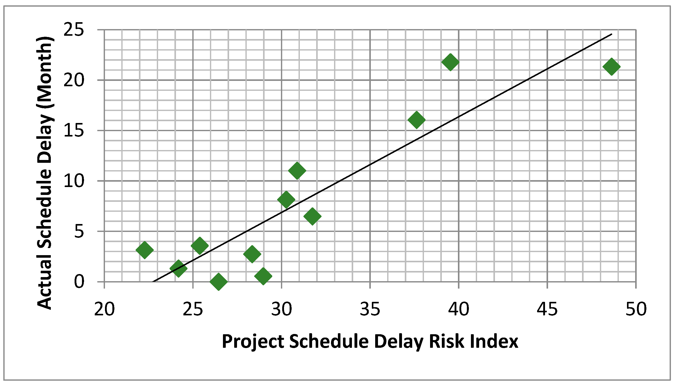
The summary of SDRI shown in Table 10 can be grouped into two off shore project types with a unique trend, similar to the schedule delay tendency. The average SDRI for 6 “Fixed” platform production off shore projects (i.e., 27.2 = 163.1/6) is about 13% lower than the average (31.2 = 374.2/12) of 12 all projects (not including project M), whereas it is much lower (about 22.5%) when compared to the one for 6 “Floater” production offshore projects. This trend of higher average SDRI score for “Floater” projects is consistent with, the more schedule delay tendency as well, as explained above, in comparison to “Fixed” projects average SDRI score and average schedule delay. This trend of correlations between schedule delay trend and SDRI score tendency strengthen the hypothesis raised in this study, that is the higher SDIR score in SOW/TDM, the tighter in owner’s requirements both in SOW and CT eventually shown in Lessons Learned reports. Therefore, the contractor should pay more attention to the risk of schedule delay in bidding and contracting stage with when the higher SDRI score is indicated in their contract documents, especially SOW. Figure 4 shows the resultant SD-SDRIs scatter plot. As can be seen from this, a linear correlation appears to adequately estimate the relationship.
Table 11 shows the resultant SDEM based on the SD-SDRIs regression analysis. The SDEM regression function is the line as is represented in Figure 4, above. The resultant p-value (p < 0.001) indicates that the finding is statically significant. The high R2 value of 0.8 suggests that the function is a relatively good fit for the relationship which is supported by the low appearance of variance from the resultant line as represented in Figure 4. In summary, the function appears to adequately estimate the relationship. Thus, it is likely that the SDRI value, frequency of occurrence of CTs, is a decent indicator of the schedule performance expected on an offshore O&G EPC project. It is interesting to note that when there are no CTs within the SOW documents, x equals zero, the expected SD is a 21.6-month acceleration, y equals −21.6. This is also an indicator of the impact the work associated with the CTs has on a project schedule.
Table 11 also shows the validity of the normality, independence, and homoscedasticity. The Shapiro-Wilk test resulted in a W of 0.970. The null hypothesis of the Shapiro-Wilk test is that the observations follow a normal distribution. As the null hypothesis cannot be rejected at the significance level of 5 percent (p = 0.9133), the model can be considered normally distributed. The Durbin-Watson test validates whether the autocorrelation parameter is zero or not, so that if the autocorrelation parameter is zero, the residuals are independent each other. The Durbin-Watson resulted in a D = 2.6027 and p = 0.91. Here, the D value is always greater than or equal to 0, and less than or equal to 4, and the closer to 2, the autocorrelation parameter becomes 0. According to Durbin-Watson’s autocorrelation criterion, the autocorrelation parameter can be viewed as 0, therefore the residuals is proved independent. The results of the Breusch-Pagan test using the statistical tool R were Chi-square = 0.376. The null hypothesis cannot be rejected at the significance level of 5% (p = 0.540) which confirms homoscedasticity. Thus, the assumption of normality, independence, and homoscedasticity were valid, and the model is statistically relevant.
4.2. Model Verification
To test the model, the authors then used the regression formula to predict the SD for Project M, which was completed recently by the offshore EPC contractor, comparing it to actually incurred value. The SDRI of Project M was estimated to be 37.7. Entering this into the SDEM regression formula, it is predicted that the project duration for Project M would increase by 14.2 months, as seen in Equation (5).
where, X is the SDRI of Project M (37.7) and Y is the estimated SD (14.2 months).
Y = 0.9494X − 21.6099 = 14.2 Months
Thus, according to the model prediction, Project M is expected to be delayed (SD) by 14.2 months from the planned contractual sail-away date of 28 August, 2017. In case of Project M in the offshore EPC contractor’s record, the actual increase (delay) in project duration was 11.9 months, considering the actual sail-away date of 20 August, 2018. Therefore, it is verified that the increase of project duration was predicted with an accuracy of 80.7% referencing that the difference between predicted and actual increase in project duration is only 2.3 months as summarized in Table 12.
It is worthwhile to compare the schedule delay from the predictive model (SDRI) and the DECRIS model [20] to forecast construction duration delay, as Project M was used to verify model accuracy in both publications. The DECRIS model forecasted the construction schedule delay of about 8 months (i.e., 235 days), compared to about 14 months of schedule delay from the SDEM predictive model in this paper versus 12 months of actual measured delay [20]. As can be seen, the presented SDEM model is more conservative and more accurate than the DECRIS model.
5. Conclusions
The main objective of this research is to aid contractors in knowing the level of schedule delay (SD) risks on offshore EPC O&G projects that they are considering bidding on. To achieve this goal, the authors collected the contractual scope of work (SOW) documents from thirteen projects, and interviewed subject matter experts based on lessons learned of each project to identify the impactful words or phrases (critical terms, CT) likely to be included in said SOW. From this analysis, a schedule delay estimate model (SDEM) was developed which predicts a project’s SD through schedule delay risk index (SDRI) scoring based on the summation of the normalized scores of CTs included in each project SOW. The study used the text mining process, conducting the research methodology in the order of importing data, pre-processing, structuring, and normalizing. Upon normalizing the CT scores, SDRI scoring of each of the 12 projects was surmised. Finally, the SDEM was developed through regression analysis of the SDRI and actual SD of said sample projects. The SDEM was validated by applying it to the 13th case study, resulting in an estimated SD of 14.2 months, 2.3 months greater than the actual increase with an 80.7% estimation accuracy.
Through this study, it was shown that a project SD tends to increase as the SDRI for the project increases. This suggests that the higher the SDRI is, the more various problems arise in the project requiring unanticipated additional time to solve them or the greater the scheduling risks. The SDEM potentially assists contractor’s decision-makers in determining whether or not to bid on a project. Furthermore, if the contractor decides to bid, it may aid said contractor in accurately estimating potential project risks and ensuring the project schedule is attainable in the final contracts. The term document matrix, used to graphically represent all terms including CTs and their frequencies in the SOW, can aid contractors to understand what the most likely risks and their relative impact on project success are. This will likely aid them through their risk assessment process, empowering them to discuss mitigation plans to lower project risks and prevent SDs. This study’s methodology can be generalized and employed in other industries as long as information regarding both lessons learned and the contractor’s SOW are available for analysis.
This study contributes in the following five aspects. First, the authors suggest a new methodology to utilize text mining and information regarding lessons-learned in predicting construction delay. According to the authors’ literature review, there were no cases of using text mining and information regarding lessons-learned to predict the construction duration. The unique research methodology was accomplished by combining the advantages of advanced text mining technologies and the lesson-learned information as the accumulation of organizational assets. Second, it becomes possible to review the appropriateness of contact duration through SOW within a short time before its contract. Similarity estimation or parameter estimation methods are not applicable in a short time where there is lack of a detail project information or it depends on some project parameters to predict construction duration. However, this study predicts the construction duration based on the contract document SOW, which defined the scope of the contractor’s work, so it is more reliable than the above estimation methods to examine the appropriateness of the construction duration and delay for most projects. Third, the construction delay is predicted in quantitative presentation by the regression model developed in this study. Fourth, this study emphasizes the need for archiving and organizing lessons-learned information. When the systematic accumulation of vast project data becomes available, the main keywords collected will lead to the improvement of research. Finally, it can be used to analyze new construction risks and prepare countermeasures by examining lessons-learned information related to major keywords when construction delay is expected.
Future Research and Limitations
This study’s major limitation is the lack of data. The resultant model was based on the SOW and schedule performance of 12 projects. To increase the accuracy of this study, more projects should be collected. However, offshore O&G projects are infrequent and increasing the number of projects likely equates to increasing the countries involved, thus increasing the variables and uncertainty of the analysis. Though the end result is limited to the data collected, and likely only applicable to South Korean and similar nations, the methodology involved in attaining the model is of merit, and thus applicable to worldwide offshore O&G projects and even other sectors.
This study’s findings focused on, and therefore limited to, the bidding stage and SOWs. The methodology could be modified to estimate the schedule performance at the engineering, procurement, and construction phases. This would simply require the text mining focus to be changed from the SOW to other contractual documents, such as the conditions of the contract, exhibits and annex etc. specific for those phases, which is likely to improve a level of SDRI. In addition, Lessons learned created for contractor’s good performance in the yard can also be collected, that will cause SDRI to be balanced by making it decreased.
Also, this study makes the assumption that all CTs are of equal impact to schedule risk. This is an oversimplification based on the assumption that a CT equates to a risk and the risk’s impact is only described by the probability of its occurrence. This eliminates the consideration of a risk’s variability to impact. For example, the term “escape tunnel” likely has a greater impact on the schedule than “nozzle”. While this remains a limitation, using count data to develop risk scoring has been used historically in the literature [20,21,33,44].
Finally, research utilizing the meaning of each text itself may be considered for future study. For example, on one project, a contractor is contractually allowed fourteen days to review a document, and on another project seven days is only given to review a document, different risks of project schedule delays are anticipated caused by different review periods or the maturity of engineering documents. Therefore, a study to reflect the context of some texts in addition to normalized text frequencies is also recommended.
Abbreviation
| CT | Critical Term |
| DLD | Delay Liquidated Damages |
| DECRIS | Detail Engineering Completion Rating Index System |
| EPC | Engineering, Procurement and Construction |
| ERP | Enterprise Resource Planning |
| FPSO | Floating Production, Storage and Offloading |
| O&G | Oil and Gas |
| PDRI | Project Definition Rating Index |
| SD | Schedule Delay |
| SDEM | Schedule Delay Estimate Model |
| SDRI | Schedule Delay Risk Index |
| SME | Subject Matter Expert |
| SOW | Scope of Work |
| TDM | Term Document Matrix |
| TF | Term Frequency |
| TOC | Table of Contents |
Author Contributions
The contribution of the authors for this publication article are as follows: conceptualization, B.-Y.S. and E.-B.L.; methodology, B.-Y.S.; software, B.-Y.S.; validation, E.-B.L.; formal analysis, B.-Y.S.; writing—original draft preparation, B.-Y.S.; writing—review and editing, E.-B.L.; visualization, B.-Y.S.; supervision, E.-B.L.; project administration, E.-B.L.; and funding acquisition, E.-B.L. If desired, refer to the Contributor Roles Taxonomy (CRediT taxonomy https://www.casrai.org/credit.html) for more detailed explanations of the authors contributions. All the authors read and approved the final manuscript.
Funding
The authors acknowledge that this research was sponsored by the Ministry of Trade Industry and Energy (MOTIE/KEIT) Korea through the Technology Innovation Program funding for: (1) Artificial Intelligence Big-data (AI-BD) Platform for Engineering Decision-support Systems (grant number = 20002806); and (2) Intelligent Project Management Information Systems (i-PMIS) for Engineering Projects (grant number = 10077606).
Acknowledgments
The authors would like to thank J.H.L. (a graduate student at POSTECH Univ.), C.M.K. (a senior researcher at Univ. of California at Davis) and D.S.A. (a Ph. D. candidate in Univ. of Colorado at Boulder) for their academic inputs and feedback on this research. The views expressed in this paper are solely those of the authors and do not represent those of any official organization.
Conflicts of Interest
The authors declare no conflict of interest. The funders had no role in the design of the study; in the collection, analyses, or interpretation of data; in the writing of the manuscript, or in the decision to publish the results.
Appendix A. Example of EPC Contract and Its Exhibits List

Table A1.
Condition of Contract: Article List.
| No. | Article * | No. | Article * |
|---|---|---|---|
| 1 | Definitions And Interpretation | 14 | Insurance |
| 2 | Relationships and Acknowledgements | 15 | Documentation |
| 3 | Obligations of Contractor | 16 | Completion |
| 4 | Feed Document, Design and Technology | 17 | Inspection and Warranty |
| 5 | Obligations of Owner | 18 | Assignment and Guarantee |
| 6 | Representations of the parties | 19 | Subcontracting |
| 7 | Taxes | 20 | Guarantee of Timely Completion |
| 8 | Measurement | 21 | Default, Termination and Suspension |
| 9 | Contract Price | 22 | Indemnities; Limitations of Liability |
| 10 | Payments to Contractor | 23 | Force Majeure |
| 11 | Commencement of Work: Project Schedule | 24 | Dispute Resolution |
| 12 | Change Orders | 25 | Miscellaneous Provisions |
| 13 | Title and Risk of Loss | 26 | Additional Considerations |
(* note: due to a space limit, only highest level of Articles is listed without its sub-articles.)
Table A2.
Exhibit List.
| No. | Exhibit | No. | Exhibit |
|---|---|---|---|
| 1 | Scope of Work*
| 17 | Project Schedule |
| 2 | FEED Dossier | 18 | Form of Change Order |
| 3 | Directives for Engineering Services | 19 | Form of Plant Acceptance Certificate |
| 4 | Directives for Construction and Assembly | 20 | Insurance Requirements |
| 5 | Directives for Procurement | 21 | Form of Ready for Start Up Certificate |
| 6 | Directives for Planning and Control | 22 | Form of Handover Certificate |
| 7 | Directives for Quality Assurance System | 23 | Form of Final Lien Waiver |
| 8 | Directives for Commissioning | 24 | Performance Security |
| 9 | Directives for Health, Safety and Environment | 25 | Form of Substantial Completion Certificate |
| 10 | Facilities for Owner’s Representatives | 26 | Form of Final Completion Certificate |
| 11 | Contractor Consents and Permits | 27 | Form of Plant Acceptance Certificate |
| 12 | Owner Consents and Permits | 28 | Pre-EPC Contract |
| 13 | Administrational Structure Outline | 29 | Technical Proposal |
| 14 | Lump Sum Price Distribution | 30 | Commercial Proposal |
| 15 | Price Schedule | 31 | Request for Proposal # 0082076118- Bidding Process 2 |
| 16 | Measurement Criteria |
(* note: due to a space limit, only highest level of Exhibit is listed without its sub-articles, except SOW).
Appendix B. List of Critical Terms Shown on SOW, Included in TDM/SDRI (Total 282* Texts in Alphabetical Order)
| align * | flange_management | material_handling | sea_trial |
| alignment * | flatness | material_handling_equipment | sil |
| aluminium | flush * | mct * | site_acceptance |
| aluminum | fusible | medical | slop * |
| analyser * | global_design | meggar | slope * |
| analyzer * | government | megger | solas |
| approved_supplier * | grated * | mill | splash * |
| approved_vendor * | gre | mill_certificate * | standardization |
| atex | gre_pipe * | misalignment | stenciled * |
| baseline | gre_piping | mock | stroke_test * |
| baseline_inspection * | grillage * | monorail * | sunshade * |
| baseline_survey * | grp_grating | moorings | switchboard * |
| blast | handling_equipment * | multi_cable_transit * | swivel |
| blast_loading * | hardness | nigerian * | tendon * |
| bulletin * | heat_tracing | noise | thruster * |
| cable_tray * | hipps | nominated | tolerance * |
| caisson * | hydraulic_control_lines | norsok | torque * |
| ce_marked * | hydraulic_lines | nozzle * | towing |
| chemical_clean * | icaps | oil_flush * | tubing |
| coaming * | heat_tracing | opercom | turret |
| color_coded * | hipps | padeye * | ucp* |
| colour_code* | hydraulic_control_lines | passive_fire_protection | ukcs |
| consortium | hydraulic_lines | ped | unit_control_panel * |
| constructability | icaps | pedestal | variable_frequency_drive * |
| cpi | iecex | petroleum_safety_authority | vent_boom * |
| critical_line * | ifat * | pfp | vfd * |
| davit * | impact_test * | piping_stress | vibration * |
| deck_drain * | import_permit * | pneumatic | water_ponds |
| deluge | inergen | pob | weather |
| diesel_engine * | information_management | post_weld_heat_treatment | weighing |
| dispersion | insulation | pre_qualification * | weld_overlay |
| dispersion_study | lci | procosys | weld_repair |
| dosh | lcs | project_completion_system | winch * |
| double_door | leak_test * | psa | winterisation |
| dry | level_bridles | ptb * | winterization * |
| enclosure * | license * | pwht | work_permit |
| endurance_test * | lifting_appliances | raised_floor * | working_environment * |
| enhanced_oil_recovery | lifting_equipment * | re_calibration | |
| eor | lli | receiving_inspection * | |
| escape_route * | load_test * | removable | |
| escape_tunnel | local_content * | removable_spool * | |
| explosion_proof | local_control_station * | retest * | |
| fibre_optic * | local_regulation * | running_test * | |
| final_document * | loler | safety_sign * | |
| final_documentation * | loop_test * | sarawak | |
| final_dossiers | lsa | sat | |
| flame_detector * | mac | sea_fasten * | |
| (note: * indicates representative alphabetical character to simplify CT numbers for a simplicity purpose). | |||
Appendix C. List of Critical Terms NOT Shown on SOW, Excluded in TDM/SDRI (Total 25 Texts in Alphabetical Order)
| avm | festoon | peelable_coating | straight_distance |
| bending_pin | full_atex | preroll | straight_length |
| bladder | jack_screw | retardant_sleeve | tubing_length |
| bosiet | lifting_operation_plan | retractable_davit | ul_listed |
| capstan | mcmc | rtj | |
| crane_adaptor | nuclear | safety_gate | |
| fcaw | osp | slide_shoe |
Appendix D. List of Stop Words: 174 Words
| a | for | more | themselves | why’s |
| about | from | most | then | with |
| above | further | mustn’t | there | won’t |
| after | had | my | there’s | would |
| again | hadn’t | myself | these | wouldn’t |
| against | has | no | they | you |
| all | hasn’t | nor | they’d | you’d |
| am | have | not | they’ll | you’ll |
| an | haven’t | of | they’re | your |
| and | having | off | they’ve | you’re |
| any | he | on | this | yours |
| are | he’d | once | those | yourself |
| aren’t | he’ll | only | through | yourselves |
| as | her | or | to | you’ve |
| at | here | other | too | |
| be | here’s | ought | under | |
| because | hers | our | until | |
| been | herself | ours | up | |
| before | he’s | ourselves | very | |
| being | him | out | was | |
| below | himself | over | wasn’t | |
| between | his | own | we | |
| both | how | same | we’d | |
| but | how’s | shan’t | we’ll | |
| by | I | she | we’re | |
| cannot | i’d | she’d | were | |
| can’t | if | she’ll | weren’t | |
| could | i’ll | she’s | we’ve | |
| couldn’t | i’m | should | what | |
| did | in | shouldn’t | what’s | |
| didn’t | into | so | when | |
| do | is | some | when’s | |
| does | isn’t | such | where | |
| doesn’t | it | than | where’s | |
| doing | it’s | that | which | |
| don’t | its | that’s | while | |
| down | itself | the | who | |
| during | i’ve | their | whom | |
| each | let’s | theirs | who’s | |
| few | me | them | why |
Appendix E. List of Example of Normalized TDM (Number Indicates Normalized Appearance Number in SOW)
| TDM/Project | PJT_A | PJT_B | PJT_C | PJT_D | PJT_E | PJT_F | PJT_G | PJT_H | PJT_I | PJT_J | PJT_K | PJT_L | PJT_M |
| … | … | … | … | … | … | … | … | … | … | … | … | … | … |
| application | 0.588 | 0.528 | 0.29 | 0.446 | 2.336 | 0.303 | 0 | 0.536 | 0.635 | 0.908 | 0.446 | 0.623 | 0.539 |
| applications | 0.353 | 0.264 | 0.097 | 0.446 | 0.076 | 0.152 | 0 | 0.383 | 0.127 | 0 | 0.891 | 0.089 | 0.071 |
| applicator | 0 | 0 | 0 | 0 | 0.151 | 0 | 0 | 0 | 0.043 | 0 | 0 | 0 | 0 |
| applied | 0.705 | 0.528 | 0.194 | 0.446 | 0.453 | 0.152 | 0.263 | 0.459 | 1.27 | 0.303 | 0.179 | 1.157 | 0.305 |
| applies | 0.235 | 0.176 | 0 | 0 | 0.076 | 0 | 0.263 | 0.039 | 0.127 | 0 | 0.179 | 0 | 0.071 |
| apply | 1.644 | 1.848 | 0.29 | 1.484 | 0.377 | 0.454 | 1.84 | 0.23 | 0.339 | 1.009 | 0.624 | 0.445 | 0.305 |
| applying | 0 | 0 | 0 | 0 | 0.076 | 0 | 0.526 | 0 | 0.043 | 0.202 | 0 | 0.045 | 0.047 |
| appoint | 0.47 | 0.352 | 0.29 | 0.149 | 0.377 | 0.454 | 0.263 | 0.039 | 0.212 | 0.101 | 0.179 | 0.267 | 0.422 |
| appointed | 0.353 | 0.352 | 0.194 | 0.891 | 0.302 | 0.605 | 1.052 | 0 | 0.17 | 0.101 | 0.802 | 0.178 | 0.468 |
| appointment | 0 | 0 | 0 | 0 | 0.076 | 0 | 0 | 0 | 0.085 | 0.101 | 0 | 0 | 0.071 |
| appraisal | 0.118 | 0.088 | 0 | 0.149 | 0.151 | 0 | 0 | 0 | 0.551 | 0.101 | 0 | 0.089 | 0.047 |
| appraisals | 0 | 0 | 0 | 0 | 0 | 0 | 0 | 0 | 0.043 | 0 | 0 | 0.045 | 0 |
| approach | 0 | 0 | 0 | 0 | 0.076 | 0.303 | 0.526 | 1.415 | 1.016 | 0.101 | 0.357 | 0.356 | 0.585 |
| approaches | 0 | 0 | 0 | 0 | 0 | 0 | 0 | 0.421 | 0.043 | 0.101 | 0 | 0 | 0.071 |
| approaching | 0 | 0 | 0 | 0 | 0 | 0 | 0 | 0 | 0 | 0 | 0 | 0 | 0.024 |
| appropriately | 0 | 0 | 0 | 0 | 0.076 | 0 | 0 | 0.077 | 0.212 | 0.202 | 0 | 0.089 | 0.024 |
| appropriateness | 0 | 0 | 0 | 0 | 0 | 0 | 0 | 0 | 0 | 0 | 0 | 0 | 0.024 |
| approvability | 0 | 0 | 0 | 0 | 0 | 0 | 0 | 0 | 0.043 | 0 | 0 | 0 | 0 |
| approvals | 1.527 | 1.144 | 0 | 0.594 | 0.377 | 0.303 | 0.263 | 0.077 | 0.297 | 0.404 | 0.09 | 0.89 | 0.281 |
| approve | 0.94 | 0.616 | 0.29 | 1.039 | 0.377 | 0.152 | 2.103 | 0.077 | 0.424 | 0.606 | 0.179 | 0.579 | 0.351 |
| approved_supplier | 0 | 0 | 0 | 0 | 0 | 0 | 0 | 0 | 0.085 | 0 | 0 | 0 | 0.047 |
| approved_suppliers | 0 | 0 | 0 | 0 | 0 | 0 | 0 | 0 | 0 | 0 | 0 | 0 | 0.071 |
| approved_vendor | 0.118 | 0 | 0 | 0 | 0.151 | 0 | 0 | 0.039 | 0.381 | 0 | 0 | 0.045 | 0.281 |
| approved_vendors | 0.235 | 0.088 | 0 | 0.149 | 0.076 | 0.303 | 0 | 0 | 0 | 0.101 | 0 | 0.178 | 0.164 |
| … | … | … | … | … | … | … | … | … | … | … | … | … | … |
| sub-total | 1000 | 1000 | 1000 | 1000 | 1000 | 1000 | 1000 | 1000 | 1000 | 1000 | 1000 | 1000 | 1000 |
References
- KEEI. 2016 Long-Term Energyforecasting; Korea Energy Economics Institute: Ulsan, Korea, 2016; pp. 1–159. [Google Scholar] [CrossRef]
- Do, H.J. Tasks and Countermeasures of the Domestic Resource Development Offshore Plant Industry; Korea Energy Economics Institute: Ulsan, Korea, 2015; pp. 1–113. [Google Scholar]
- Johansen, A.; Landmark, A.D.; Olshausen, F.; van der Kooij, R.; Skappel, S. Time elasticity-who and what determines the correct project duration. Procedia Comput. Sci. 2016, 100, 586–593. [Google Scholar] [CrossRef]
- Douglas-Westwood. FPSO Industry Must Re-Think Supply Chain. Available online: https://www.offshore-mag.com/articles/print/volume-74/issue-2/fpso-outlook/fpso-industry-must-re-think-supply-chain.html (accessed on 2 May 2019).
- Project Management Institute (PMI). A Guide to the Project Management Body of Knowledge, 6th ed.; Project Management Institute: Newtown Square, PA, USA, 2017; ISBN 10: 9781628251845. [Google Scholar]
- Rawash, A.; El Hagla, K.; Bakr, A. Heuristic approach for risk assessment modeling: EPCCM application (engineer procure construct contract management). J. Mod. Sci. Technol. 2014, 2, 49–70. [Google Scholar] [CrossRef]
- Yeo, K.; Ning, J. Integrating supply chain and critical chain concepts in engineer-procure-construct (EPC) projects. Int. J. Proj. Manag. 2002, 20, 253–262. [Google Scholar] [CrossRef]
- Bevilacqua, M.; Ciarapica, F.; Giacchetta, G. Critical chain and risk analysis applied to high-risk industry maintenance: A case study. Int. J. Proj. Manag. 2009, 27, 419–432. [Google Scholar] [CrossRef]
- Öztaş, A.; Ökmen, Ö. Risk analysis in fixed-price design–build construction projects. Build. Environ. 2004, 39, 229–237. [Google Scholar] [CrossRef]
- Bali, R.; Apte, M.R. Risk management in EPC contract—Risk identification. J. Mech. Civ. Eng. 2014, 11, 7–12. [Google Scholar] [CrossRef]
- Odeh, A.M.; Battaineh, H.T. Causes of construction delay: Traditional contracts. Int. J. Proj. Manag. 2002, 20, 67–73. [Google Scholar] [CrossRef]
- Gebrehiwet, T.; Luo, H. Analysis of delay impact on construction project based on RII and correlation coefficient: Empirical study. Procedia Eng. 2017, 196, 366–374. [Google Scholar] [CrossRef]
- Alsakini, W.; Wikström, K.; Kiiras, J. Proactive schedule management of industrial turnkey projects in developing countries. Int. J. Proj. Manag. 2004, 22, 75–85. [Google Scholar] [CrossRef]
- Ahsan, K.; Gunawan, I. Analysis of cost and schedule performance of international development projects. Int. J. Proj. Manag. 2010, 28, 68–78. [Google Scholar] [CrossRef]
- Chang, A.S.T. Reasons for cost and schedule increase for engineering design projects. J. Manag. Eng. 2002, 18, 29–36. [Google Scholar] [CrossRef]
- Assaf, S.A.; Al-Hejji, S. Causes of delay in large construction projects. Int. J. Proj. Manag. 2006, 24, 349–357. [Google Scholar] [CrossRef]
- Shrestha, P.P.; Burns, L.A.; Shields, D.R. Magnitude of construction cost and schedule overruns in public work projects. J. Constr. Eng. 2013, 2013, 9. [Google Scholar] [CrossRef]
- Olawale, Y.A.; Sun, M. Cost and time control of construction projects: Inhibiting factors and mitigating measures in practice. Constr. Manag. Econ. 2010, 28, 509–526. [Google Scholar] [CrossRef]
- Iyer, K.C.; Chaphalkar, N.B.; Joshi, G.A. Understanding time delay disputes in construction contracts. Int. J. Proj. Manag. 2008, 26, 174–184. [Google Scholar] [CrossRef]
- Kim, M.H.; Lee, E.B.; Choi, H.S. A forecast and mitigation model of construction performance by assessing detailed engineering maturity at key milestones for offshore epc mega-projects. Sustainability 2019, 11, 1256. [Google Scholar] [CrossRef]
- Kim, M.H.; Lee, E.B.; Choi, H.S. Detail engineering completion rating index system (DECRIS) for optimal initiation of construction works to improve contractors’ schedule-cost performance for offshore oil and gas EPC projects. Sustainability 2018, 10, 2469. [Google Scholar] [CrossRef]
- Jo, S.H.; Lee, E.B.; Pyo, K.Y. Integrating a procurement management process into critical chain project management (CCPM): A case-study on oil and gas projects, the piping process. Sustainability 2018, 10, 1817. [Google Scholar] [CrossRef]
- Welbers, K. Gatekeeping in the Digital Age. Ph.D. Thesis, Vrije Universiteit, Amsterdam, The Netherlands, 2016. [Google Scholar]
- Miner, G.; Elder, J.I.V.; Fast, A.; Hill, T.; Nisbet, R.; Delen, D. Practical Text Mining and Statistical Analysis for Non-Structured Text Data Applications; Elsevier Science & Technology: Saint Louis, LA, USA, 2012; ISBN 978-0-12-386979-1. [Google Scholar]
- Hearst, M.A. Untangling text data mining. In Proceedings of the 37th Annual Meeting of the Association for Computational Linguistics on Computational Linguistics, College Park, MD, USA, 20–26 June 1999; pp. 3–10. [Google Scholar] [CrossRef]
- Ur-Rahman, N.; Harding, J.A. Textual data mining for industrial knowledge management and text classification: A business oriented approach. Expert Syst. Appl. 2012, 39, 4729–4739. [Google Scholar] [CrossRef] [Green Version]
- Singh, S.; Yassine, A. Big data mining of energy time series for behavioral analytics and energy consumption forecasting. Energies 2018, 11, 452. [Google Scholar] [CrossRef]
- Weiss, S.M.; Indurkhya, N.; Zhang, T. Fundamentals of Predictive Text Mining, 2nd ed.; Springer: New York, NY, USA, 2015; ISBN 13: 978-1447167495. [Google Scholar]
- Wang, H.C.; Chi, Y.C.; Hsin, P.L. Constructing patent maps using text mining to sustainably detect potential technological opportunities. Sustainability 2018, 10, 3729. [Google Scholar] [CrossRef]
- Fan, H.; Li, H. Retrieving similar cases for alternative dispute resolution in construction accidents using text mining techniques. Autom. Constr. 2013, 34, 85–91. [Google Scholar] [CrossRef]
- Shen, L.; Yan, H.; Fan, H.; Wu, Y.; Zhang, Y. An integrated system of text mining technique and case-based reasoning (TM-CBR) for supporting green building design. Build. Environ. 2017, 124, 388–401. [Google Scholar] [CrossRef]
- Arif-Uz-Zaman, K.; Cholette, M.E.; Ma, L.; Karim, A. Extracting failure time data from industrial maintenance records using text mining. Adv. Eng. Inform. 2017, 33, 388–396. [Google Scholar] [CrossRef] [Green Version]
- Lee, J.; Yi, J.-S. Predicting project’s uncertainty risk in the bidding process by integrating unstructured text data and structured numerical data using text mining. Appl. Sci. 2017, 7, 1141. [Google Scholar] [CrossRef]
- Williams, T.P.; Gong, J. Predicting construction cost overruns using text mining, numerical data and ensemble classifiers. Autom. Constr. 2014, 43, 23–29. [Google Scholar] [CrossRef]
- Marzouk, M.; Enaba, M. Text analytics to analyze and monitor construction project contract and correspondence. Autom. Constr. 2018, 98, 265–274. [Google Scholar] [CrossRef]
- Choudhary, A.K.; Oluikpe, P.; Harding, J.A.; Carrillo, P.M. The needs and benefits of text mining applications on post-project reviews. Comput. Ind. 2009, 60, 728–740. [Google Scholar] [CrossRef]
- Pinto, T.; Vale, Z.; Praça, I.; Pires, E.J.S.; Lopes, F. Decision support for energy contracts negotiation with game theory and adaptive learning. Energies 2015, 8, 9817–9842. [Google Scholar] [CrossRef]
- Lotfian, F.; Kimiagari, A.M.; Pejmannia, S.; Keivanloo, M. Pricing policy in EPC oil & gas projects. Int. J. Trade Econ. Financ. 2010, 1, 023X. [Google Scholar] [CrossRef]
- Welbers, K.; Van Atteveldt, W.; Benoit, K. Text analysis in R. Commun. Methods Meas. 2017, 11, 245–265. [Google Scholar] [CrossRef]
- R Core Team. R: A Language and Environment for Statistical Computing; R Foundation for Statistical Computing: Vienna, Austria, 2017; Available online: https://www.R-project.org/ (accessed on 13 May 2018).
- Salton, G.; Wong, A.; Yang, C.-S. A vector space model for automatic indexing. Commun. ACM 1975, 18, 613–620. [Google Scholar] [CrossRef] [Green Version]
- Stop Words in Wikipedia.com. Available online: https://en.wikipedia.org/wiki/Stop_words (accessed on 5 May 2019).
- Misund, B. Vertical integration and value-relevance: Empirical evidence from oil and gas producers. Cogent Econ. Financ. 2016, 4, 1264107. [Google Scholar] [CrossRef]
- Gibson, G.; Dumont, P.R. Project Definition Rating Index (PDRI) for Industrial Projects; Construction Industry Institute Implementation Resource, University of Texas at Austin: Austin, TX, USA, 1996; p. 113-11. [Google Scholar]
- Lee, J.H.; Yi, J.S.; Son, J. Unstructured construction data analytics using R programming-focused on overseas construction adjudication cases. J. Archit. Inst. Korea Struct. Constr. 2016, 32, 37–44. [Google Scholar] [CrossRef]
- Lee, W.R. Introduction of Regression Analysis, 2nd ed.; Tamjin: Seoul, Korea, 2012. [Google Scholar]
Figure 1.
Business profits and losses of Korean major EPC contractors.

Figure 2.
Research flowchart. SME—Subject Matter Expert; SDRI—Schedule Delay Risk Index, CT—Critical Term, SDEM—Schedule Delay Estimate Model.
Figure 2.
Research flowchart. SME—Subject Matter Expert; SDRI—Schedule Delay Risk Index, CT—Critical Term, SDEM—Schedule Delay Estimate Model.

Figure 3.
The overall process of text mining of SOW (modified from [39]).
Figure 3.
The overall process of text mining of SOW (modified from [39]).

Figure 4.
Scatter plot (project SDRI vs. actual SD).

Table 1.
Reasons of project schedule delay by 9 FPSOs case studies (modified from [4]) (unit = month).
Table 1.
Reasons of project schedule delay by 9 FPSOs case studies (modified from [4]) (unit = month).
| Reason for Delay | Project | Total Delay Per Reason (Month) | ||||||||
|---|---|---|---|---|---|---|---|---|---|---|
| A | B | C | D | E | F | G | H | I | ||
| Integration | 3 | 1.5 | 3 | - | 3 | 1 | - | 8 | 9 | 28.5 |
| Yard Availability | - | 2 | 7 | 3 | 2 | 2 | - | 6 | - | 22 |
| Engineering Scope | 1 | 1 | 4 | 8 | 1 | 0.5 | 2 | 1 | 2 | 20.5 |
| Commissioning | 1 | 1 | - | - | - | - | 6 | 3 | - | 11 |
| Material Process | 7 | - | 4 | 2 | - | - | - | - | - | 13 |
| Equipment Package & Installation | 1 | 0.5 | 2 | 4 | - | 0.5 | 6 | - | 2 | 16 |
| Operator Contracting | - | - | 14 | - | - | - | - | - | - | 14 |
| Financing | - | - | - | - | 3 | - | - | - | - | 3 |
| Political/Unforeseen | - | - | 18 | - | - | - | - | - | - | 18 |
| Total Project Delay | 13 | 6 | 52 | 17 | 9 | 4 | 14 | 18 | 13 | 146 |
| Project Cost Growth | 23% | 26% | 50% | 80% | 138% | 167% | 103% | 52% | 59% | 38% average |
Table 2.
Sample project SOW descriptions.
| Sample Project | Type | No. of Pages (SOW) | No. of Texts a | Word Count b | Ratio c |
|---|---|---|---|---|---|
| A | Floater | 88 | 5338 | 35,467 | 6.6 |
| B | Floater | 111 | 6415 | 46,381 | 7.2 |
| C | Fixed | 182 | 5426 | 41,300 | 7.6 |
| D | Floater | 70 | 4598 | 25,816 | 5.6 |
| E | Fixed | 126 | 7096 | 53,721 | 7.6 |
| F | Fixed | 99 | 4578 | 27,626 | 6.0 |
| G | Floater | 36 | 3246 | 14,847 | 4.6 |
| H | Fixed | 236 | 11,646 | 84,339 | 7.2 |
| I | Floater | 245 | 9952 | 85,230 | 8.6 |
| J | Fixed | 95 | 5661 | 38,112 | 6.7 |
| K | Floater | 104 | 5998 | 39,413 | 6.6 |
| L | Fixed | 184 | 10,585 | 85,040 | 8.0 |
| M | Fixed | 408 | 15,905 | 150,676 | 9.5 |
a Count number of quantities of individual words; b Count number of total words included in document; c Ratio of text frequency nos. (word count) to no of texts.
Table 3.
General experience description of subject matter experts.
| Details | Number |
|---|---|
| Participants | 8 people |
| Overall Experience | 77 years |
| Over 10 years of Experience | 3 people |
| Project Management Professionals | 3 people |
| Risk Management Professionals | 2 people |
Table 4.
Top 10 words of high text frequencies among 300 frequency words removed in the SOW.
| Top Rank | Text | No. of Doc | Text Frequency | Ratio |
|---|---|---|---|---|
| 1 | shall | 13 | 16,507 | 3.6% |
| 2 | contractor | 13 | 11,899 | 2.6% |
| 3 | company | 13 | 7597 | 1.7% |
| 4 | work | 13 | 7272 | 1.6% |
| 5 | equipment | 13 | 4617 | 1.0% |
| 6 | commissioning | 13 | 3495 | 0.8% |
| 7 | design | 13 | 3142 | 0.7% |
| 8 | system | 13 | 3111 | 0.7% |
| 9 | contract | 13 | 3050 | 0.7% |
| 10 | brz | 1 | 2999 | 0.7% |
Table 5.
Comparison of CT with non-CT according to text frequency in SOW.
| Text Frequency | CT | Non-CT a | ||||
|---|---|---|---|---|---|---|
| No. of Text | Total Word Count | No. of Text | Total Word Count | |||
| 1–99 | 264 | 3419 | 54% | 9462 | 105,478 | 23% |
| 100–199 | 14 | 1938 | 31% | 349 | 49,034 | 11% |
| 200–299 | 4 | 938 | 15% | 147 | 36,038 | 8% |
| 300–16,507 | 0 | 0 | 0% | 278 | 261,715 | 58% |
| Total | 282 | 6295 | 100% | 10,236 | 452,265 | 100% |
a All texts except for CTs are considered as non-CT.
Table 6.
Before/after pre-processing of text data.
| Description | Quantity | |
|---|---|---|
| Number of Projects | 13 projects | |
| Number of Documents | 13 docs | |
| Number of Pages in Total | 1984 pages | |
| Word Count | Before pre-processing | 727,968 words |
| After pre-processing step 1 a,b | 458,560 words | |
| After pre-processing step 2 a,c | 196,845 words | |
| Min. Text Length after pre-processing | 3 digits | |
a Includes single words along with bi and trigram results. b 1st step: removal of stopwords, numbers, punctuations. N-gram processes also used. c 2nd step: removal of texts whose frequency over 300 times.
Table 7.
Example Term Document Matrix.
| DOC 1 | DOC 2 | DOC 3 | DOC 4 | DOC n | |
|---|---|---|---|---|---|
| TERM 1 | TF1,1 | TF1,2 | … | … | … |
| TERM 2 | TF2,1 | TF2,2 | … | … | … |
| TERM 3 | Frequencies of terms shown in each document after pre-processing | ||||
| TERM 4 | |||||
| TERM m | … | … | … | … | TFm,n |
Table 8.
Term frequency normalization example matrix.
| DOC 1 | DOC 2 | DOC 3 | DOC n | |
|---|---|---|---|---|
| TERM 1 | N1,1 | N1,2 | … | N1,n |
| TERM 2 | N2,1 | N2,2 | … | N2,n |
| … | … | … | … | … |
| TERM m | Nm,1 | … | … | Nm,n |
Table 9.
Project SDRI assessment matrix.
| CT | DOC 1 | DOC 2 | DOC n | ||
|---|---|---|---|---|---|
| TERM 1 | No | 0 | 0 | … | 0 |
| TERM 2 | Yes | N2,1 | N2,2 | … | N2,n |
| TERM 3 | Yes | N3,1 | N3,1 | … | N3,n |
| TERM 4 | No | 0 | 0 | … | 0 |
| … | … | … | … | … | … |
| TERM m | … | Nm,1 | Nm,2 | … | Nm,n |
| SDRI | … | … |
Table 10.
Sample project summary: Duration, SD, and SDRI.
| Sample Project | Type | Build Duration | Sail-Away (Completion) Date | SD (Month) | SDRI | |
|---|---|---|---|---|---|---|
| (Month) | Planned | Actual | ||||
| A | Floater | 22 | 2015-01-04 | 2015-11-30 | 11.0 | 30.9 |
| B | Floater | 35 | 2016-01-31 | 2016-10-01 | 8.1 | 30.3 |
| C | Fixed | 30 | 2017-04-26 | 2017-05-12 | 0.5 | 29.0 |
| D | Floater | 37 | 2011-03-21 | 2011-04-29 | 1.3 | 24.2 |
| E | Fixed | 27 | 2016-11-28 | 2016-11-28 | 0.0 | 26.4 |
| F | Fixed | 75 | 2013-08-11 | 2013-11-26 | 3.6 | 25.4 |
| G | Floater | 40 | 2013-05-15 | 2015-02-14 | 21.3 | 48.6 |
| H | Fixed | 29 | 2013-05-31 | 2013-09-02 | 3.1 | 22.3 |
| I | Floater | 43 | 2014-08-31 | 2015-12-25 | 16.0 | 37.6 |
| J | Fixed | 33 | 2015-04-09 | 2015-06-30 | 2.7 | 28.3 |
| K | Floater | 35 | 2015-12-15 | 2017-09-28 | 21.8 | 39.5 |
| L | Fixed | 27 | 2016-08-11 | 2017-02-21 | 6.5 | 31.7 |
| M | Fixed | 36 | 2017-08-28 | 2018-08-20 | 11.9 | Predictive * |
Table 11.
SDEM developed via regression analysis.
| SDEM (Regression Function) | Statistical Tests | |||
|---|---|---|---|---|
| Regression | Shapiro and Wilk | Durbin and Watson | Breusch-Pagan | |
| Y = 0.9494X − 21.6099 Where, X: SDRI, Y: SD | R2 = 0.815, p < 0.001 | W = 0.970, p = 0.913 | D = 2.603, p = 0.91 | Chi2 = 0.376, Df = 1, p = 0.540 |
Table 12.
Model Verification with a Case Study with Project M.
| Sample Project | SDRI | Schedule Delay (Month) | Model Accuracy | ||
|---|---|---|---|---|---|
| Estimated | Actual | Delta | |||
| M | 37.7 | 14.2 | 11.9 | 2.3 | 80.7% |
© 2019 by the authors. Licensee MDPI, Basel, Switzerland. This article is an open access article distributed under the terms and conditions of the Creative Commons Attribution (CC BY) license (http://creativecommons.org/licenses/by/4.0/).
Share and Cite
MDPI and ACS Style
Son, B.-Y.; Lee, E.-B. Using Text Mining to Estimate Schedule Delay Risk of 13 Offshore Oil and Gas EPC Case Studies During the Bidding Process. Energies 2019, 12, 1956. https://doi.org/10.3390/en12101956
AMA Style
Son B-Y, Lee E-B. Using Text Mining to Estimate Schedule Delay Risk of 13 Offshore Oil and Gas EPC Case Studies During the Bidding Process. Energies. 2019; 12(10):1956. https://doi.org/10.3390/en12101956
Chicago/Turabian StyleSon, Byung-Yun, and Eul-Bum Lee. 2019. "Using Text Mining to Estimate Schedule Delay Risk of 13 Offshore Oil and Gas EPC Case Studies During the Bidding Process" Energies 12, no. 10: 1956. https://doi.org/10.3390/en12101956
Note that from the first issue of 2016, this journal uses article numbers instead of page numbers. See further details here.