Hybrid Forecasting Model for Short-Term Wind Power Prediction Using Modified Long Short-Term Memory


1
Department of Information and Communication Engineering, Honam University, Gwangsan-gu 62399, Korea
2
Department of Electrical Engineering, Honam University, Gwangsan-gu 62399, Korea
*
Authors to whom correspondence should be addressed.
Energies 2019, 12(20), 3901; https://doi.org/10.3390/en12203901
Submission received: 8 July 2019
/
Revised: 16 September 2019
/
Accepted: 12 October 2019
/
Published: 15 October 2019
(This article belongs to the Special Issue Solar and Wind Power and Energy Forecasting)
Abstract
:Renewable energy has recently gained considerable attention. In particular, the interest in wind energy is rapidly growing globally. However, the characteristics of instability and volatility in wind energy systems also affect power systems significantly. To address these issues, many studies have been carried out to predict wind speed and power. Methods of predicting wind energy are divided into four categories: physical methods, statistical methods, artificial intelligence methods, and hybrid methods. In this study, we proposed a hybrid model using modified LSTM (Long short-term Memory) to predict short-term wind power. The data adopted by modified LSTM use the current observation data (wind power, wind direction, and wind speed) rather than previous data, which are prediction factors of wind power. The performance of modified LSTM was compared among four multivariate models, which are derived from combining the current observation data. Among multivariable models, the proposed hybrid method showed good performance in the initial stage with Model 1 (wind power) and excellent performance in the middle to late stages with Model 3 (wind power, wind speed) in the estimation of short-term wind power. The experiment results showed that the proposed model is more robust and accurate in forecasting short-term wind power than the other models.
1. Introduction
Recently, renewable energy is increasingly being discussed with the aim of phasing out coal power and nuclear power generation to address changes in the internal and external conditions, such as new climate system, Fukushima nuclear power plant accident, increasing frequency of earthquakes, and serious air pollution. Korea is announcing the ’Renewable Energy 3020’ implementation plan, which aims to achieve a 20% share of renewable energy by 2030, and is expanding the capacity of wind power facilities from 1.2 GW in 2017 to 17.7 GW in 2030. Among different sources of renewable energy, wind energy, in which wind power is converted into electric power using a wind turbine [1], has gained particular interest. However, the output of wind power varies through time and space due to various factors, such as wind speed, wind direction, and temperature. Therefore, when large-scale wind power is linked to the grid, instability of the grid arises, and effective connection of the grid becomes difficult. In other words, the maintenance of the generator, generator shutdown plan, economic dispatch, power supply plan (generator, transmission line, etc.), and electric power market bidding become important factors when wind energy is the central supply and demand generator in the power system. For this reason, it is very important to predict the output of the wind turbine considering the stability of the wind generator system, for which various studies have been conducted recently [2,3,4].
Significant amounts of research have been conducted to predict wind power in the short, medium, or long term, and the corresponding methods can be mainly divided into three categories: physical methods, data-driven methods (statistical and artificial intelligence methods), and hybrid methods [5].
(1) Physical methods predict wind power using mathematical modeling, considering weather data (air pressure map, jet stream, etc.) and environmental characteristics (temperature, humidity, topography, land use, etc.) [6]. These methods require a large amount of data because the construction of the prediction model is complicated due to the mathematical modeling of many variables and the accuracy of prediction increases in proportion to the amount of data. Therefore, the mathematical structure of the predictive model is very difficult to achieve, the calculation process is complicated, and the calculation time is lengthy. The most widely used method is the numerical weather prediction (NWP) [7]. The NWP is suitable for long-term prediction rather than short-term and medium-term prediction because of the large amount of computation.
(2) Data-driven methods predict the wind speed within a few hours through pattern analysis, which is trained based on past data. They are more suitable for predicting wind speed values within a short period of time, as the amount of past data is continuously increasing. These methods are divided into statistical methods and artificial intelligence methods. The former can achieve high accuracy in short-term prediction, but they have a disadvantage in that they cannot accurately predict the wind power due to accumulation of errors in long-term prediction. For example, among statistical methods, the auto-regression integrated moving average (ARIMA) model is a time series analysis model [8], and various approaches have been suggested to overcome the disadvantage of ARIMA [9,10] which cannot accurately predict wind power due to the aforementioned error accumulation. The latter include neural network (NN) [11], fuzzy inference [12], particle swarm optimization (PSO) [13], genetic algorithm (GA) [14], support vector machine (SVM) [15], and long short-term memory (LSTM) [16]. The artificial intelligence method has superior performance for general purpose, but it has a disadvantage in that the relationship between model elements cannot be accurately explained.
(3) Hybrid methods employ the approach of prediction by applying statistical prediction after acquiring weather forecast data through physical methods and combining physical and statistical methods. In other words, existing physical methods are more suitable for long-term prediction than local prediction because of their large scale. Data-driven methods feature high accuracy in short-term prediction but accumulate errors in long-term prediction. Therefore, existing methods suffer from a large amount of errors, and other research is under way to improve the prediction method [17,18,19,20,21]. Hybrid methods can be categorized into four types [22,23,24]: weight-based combined approach [25,26,27], data pre-processing technique based combined approach [28,29,30,31,32], parameter selection and optimization technique based combined approach [33,34,35,36], and data post-processing technique based combined approach [37]. Firstly, the strategy of the weight-based combined approach is to assign factors to models according to their performance. It is simple and easy to implement, suitable for a wide range of prediction times, and has the advantage of adapting to new data. However, it does not guarantee the best prediction along the prediction horizon, and has a disadvantage in that an additional model is necessary for determining the weight. Secondly, the purpose of the data pre-processing technique based combined approach is to forecast the subseries obtained by decomposition. The advantage of this method is that the performance is better than that of the abovementioned approaches, and it is robust against sudden changes of wind speed. However, it requires detailed mathematical knowledge of the decomposition model and has a disadvantage of slow response time to new data. Thirdly, the purpose of the parameter selection and optimization technique based combined approach is to optimize the parameters of the forecasting model. The parameters adopted for predicting wind power are meteorological factors such as temperature, humidity, precipitation, snowfall, cloud, sunshine, wind speed, and wind direction. This method features easier determination of parameters with a relatively basic structure than the two methods mentioned above. However, it is difficult to write and implement according to the knowledge of the designer. Finally, the data post-processing technique based combined approach forecasts residual errors caused by the forecasting model. Since this method considers residual errors from the model, it can provide more accurate predictions than the abovementioned three methods. However, it has a disadvantage in that the calculation time is lengthy because residual errors must be calculated.
This study adopts an approach similar to the third type of hybrid method. In other words, the input data required for wind power prediction are classified by models, which consist of multivariate models and the performance of each model is measured. We selected wind power, wind speed, and wind direction among the meteorological factors that have the greatest impact on the prediction of short-term wind power according to the characteristics of wind farms. For performance measurement, a modified LSTM was applied to the artificial intelligence technique. We analyzed the performance of the modified LSTM by model and then combined the superior models to predict the optimum wind power. Experimental data for verifying the proposed model were acquired from wind farms in Jeju Island, South Korea. The reason for selecting Jeju Island is to promote 2 GW offshore wind power for realizing ’Carbon free island Jeju by 2030’. Moreover, Jeju Island, which has diverse winds due to Jeju Island’s characteristics, has the best conditions for the verification test. Finally, in order to predict the short-term wind power efficiently, LSTM was designed using MATLAB and the prediction error was verified through root mean square error (RMSE) and mean absolute percentage error (MAPE).
The remainder of the paper is structured as follows. Section 2 describes related works on recurrent neural network (RNN) and LSTM. Section 3 explains traditional LSTM problems and solutions, proposing a modified LSTM as well as data sets and multivariate models. Section 4 analyzes the experimental environment and results for wind farms A, B, and C in Jeju Island. Finally, Section 5 presents conclusions and future research scope.
2. Related Works
2.1. Recurrent Neural Network (RNN)
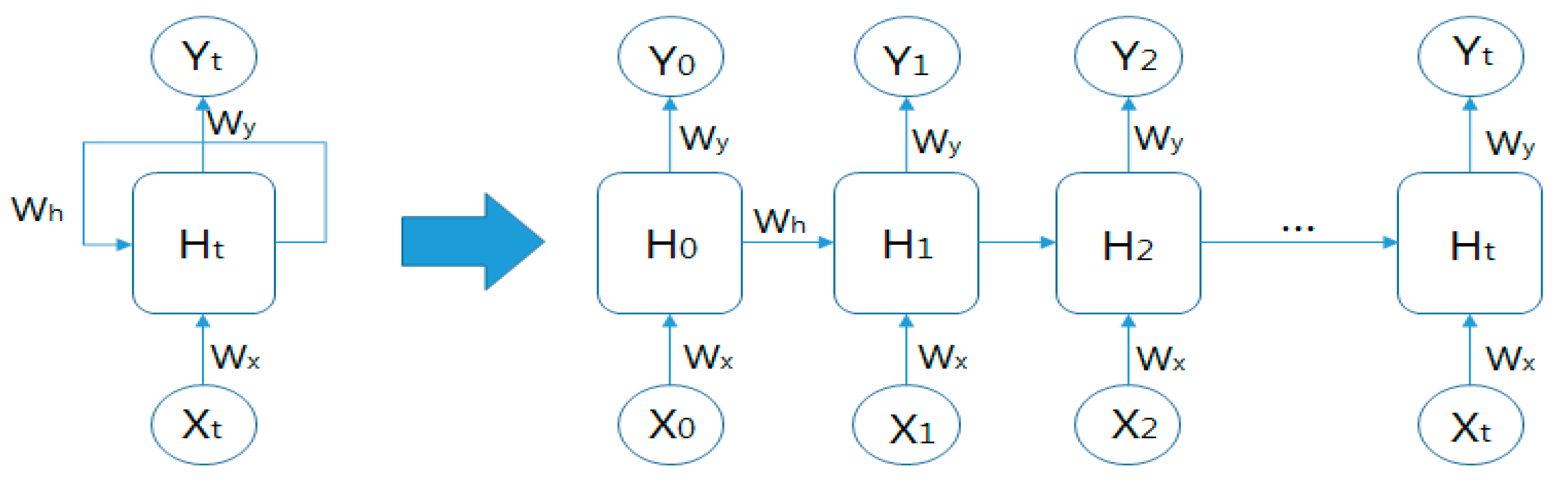
The existing neural network, Feed-Forward Neural Networks (FFNets), processes each input and output independently. In other words, when data are input, operations progress sequentially from the input layer to the hidden layer, and output is provided to the output layer. In this process, the input data are limited in that all nodes can be executed only once. However, RNN has excellent performance in a system that predicts the following states because the same process is repeated for all the input data, and the current data and all previous calculation information are applied to the current prediction result. Thus, RNN is applied to areas with outstanding performance in continuous data processing such as speech recognition, translation, language model, video, log data, and time series statistical data [38]. Figure 1 shows the RNN structure where the output of the hidden layer is input to the hidden layer again. Equation (1) is the model expression used in the hidden layer.
In Equation (1), and are the state values of the hidden layer and the output values of the output layer at time t, respectively. is a weight from the input layer, and is a weight for , which is the hidden state value of the previous time t-1. It is one of the nonlinear activation functions, and the hyperbolic tangent function (tanh) is used to calculate . is calculated using the sigmoid () function for the hidden layer state value and output layer weight at time t.
2.2. Long Short-Term Memory (LSTM)
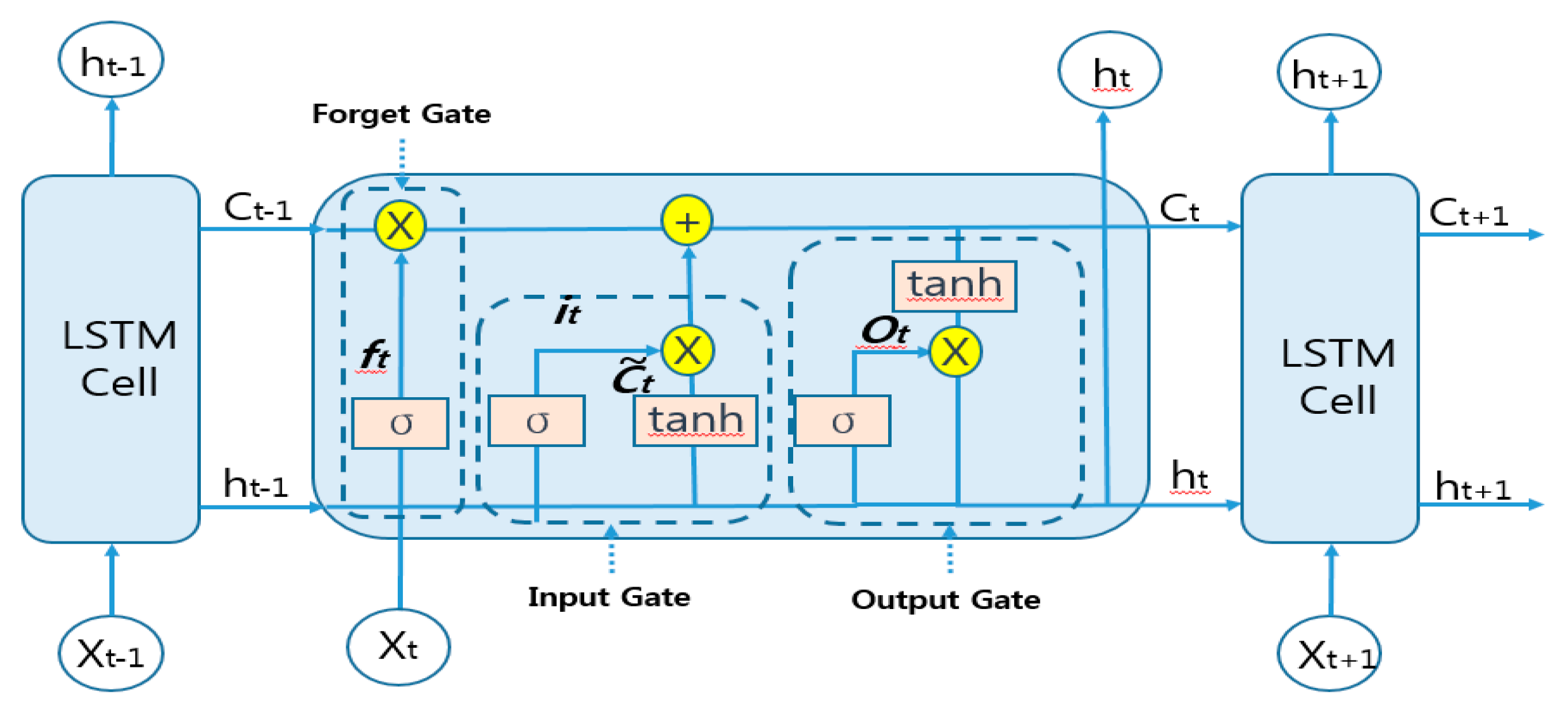
RNN has a problem of learning data over a long period of time with a vanishing gradient, where past learning results disappear if the time interval is large [39]. To solve these drawbacks, Hochreiter proposed LSTM in 1997 (Figure 2) [40]. States of LSTM cells are computed as follows:
In Equations (2)–(4), , , and are the input, forget, and output gates, respectively. As shown in Equation (5), is a new candidate value for cell state. The LSTM cell acts as an accumulator of the state information, and the update of the old cell state into the new cell state is performed using Equation (6). , , , and are weights of the input, forget, output, and current cell state, respectively. , , , and are bias of input, forget, output, and current cell state, respectively.
3. Proposed Method
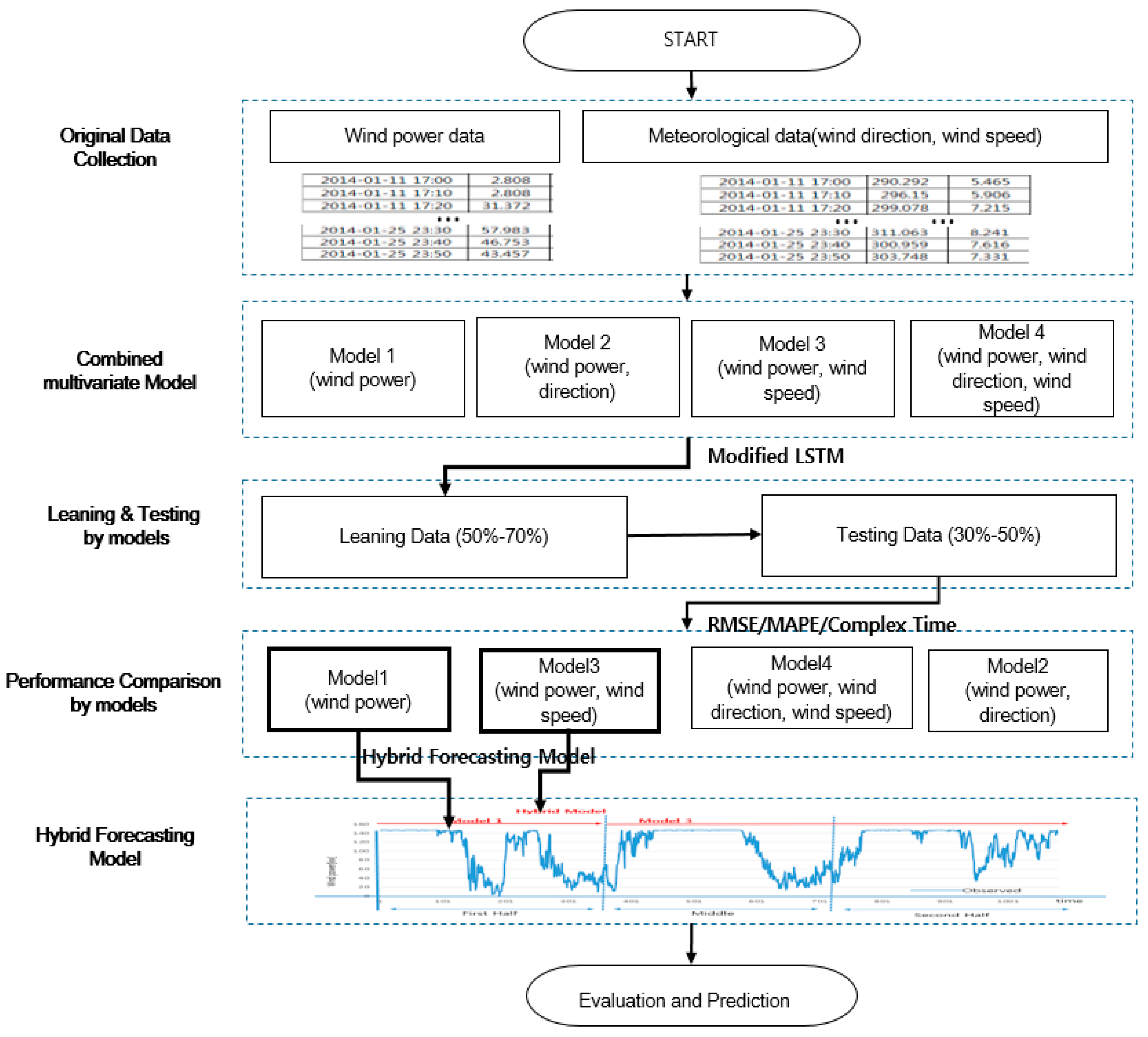
Figure 3 shows the proposed flowchart. First, wind power, wind direction, and wind speed data are collected and pre-processed. Second, multivariate models are combined by each model. Third, the proposed LSTM in Section 3.2 is applied to each model, and the performance of the model is estimated. Finally, Model 1 and Model 3, which are excellent models, are adopted and simulations are performed.
3.1. Existing LSTM Problems and Solution
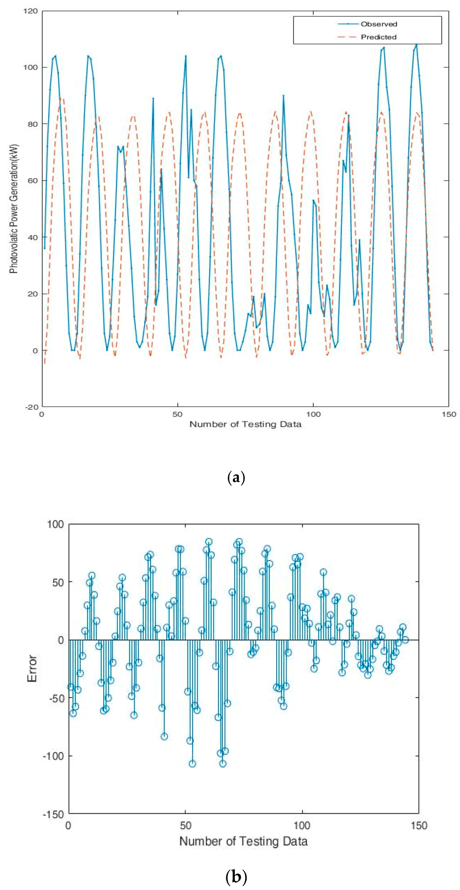
The existing LSTM uses the value of the previous prediction when forecasting the wind power value at the time steps between predictions. As shown in Figure 4, if the predicted value is incorrect, the forecast value of wind power continuously increases.
3.2. Proposed Long Short-Term Memory
In this study, since the actual value of the time steps between predictions can be accessed, the wind power is predicted by updating the network state using the observed value instead of the predicted value. Specially, the modified LSTM adopted to the input, forget, and output gates. This is because every time the LSTM proceeds, affects the input, forget, and output of the LSTM.
3.2.1. Input Gate Layer
The input gate layer receives information from the previous hidden layer and the current input. Then it computes the information to obtain an output with the following:
In Equation (8), is the output of input gate, and and are the current input and output of the previous hidden layer, respectively. and are the bias of the input gate, and . is the activation function, and the following soft function is adopted:
3.2.2. Forget Gate Layer
The output of the forget gate has a similar computation formula as the input gate with different weights and bias as shown in Equation (10).
3.2.3. Cell State Update
It is a step of updating from the previous cell state () to the current cell state (), as shown in Equation (11).
3.2.4. Output Gate Layer
As shown Equation (12), its results are decided by the current input and memory and output of the previous hidden layer.
In Equation (12), , , and indicate the outputs of the gate, current hidden layer, and bias for , respectively.
3.2.5. Learning Options and Simulation Result
LSTM has 200 hidden layers. The initial learning rate is 0.005, and the maximum number of iterations is fixed at 250. To prevent the gradients from exploding, set the gradient threshold to 1, and drop the learning rate after 125 epochs by multiplying by a factor of 0.2.
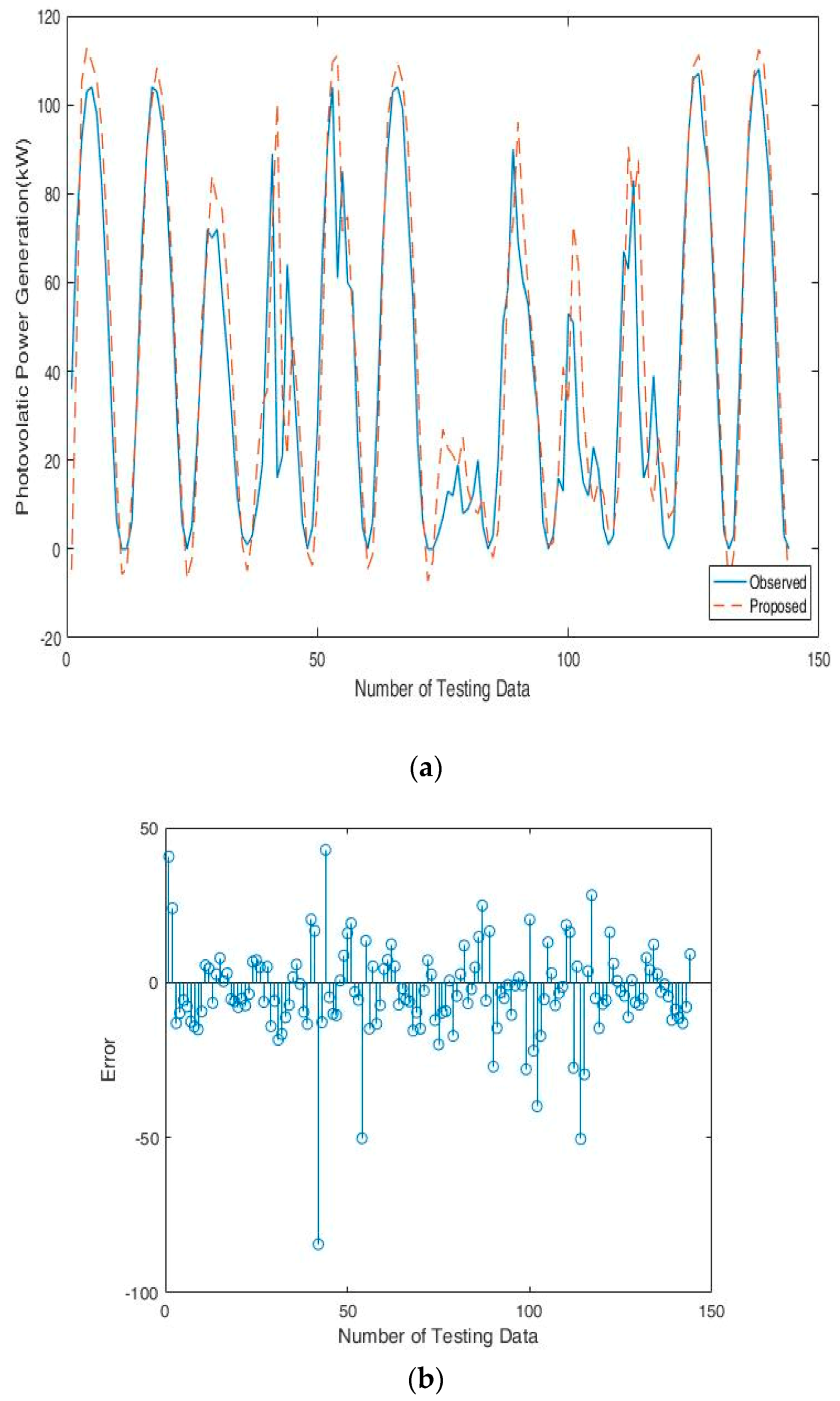
As shown in Figure 5, the predictions are more accurate when updating the network state with the observed values instead of the predicted values.
3.3. Data Set
In this study, the learning data and testing data were tested based on the wind power, wind direction, and wind speed data collected from wind farms in regions A, B, and C in Jeju Island in order to predict the short-term wind power. At this time, the learning data and the test data are all normalized data, and the collection period, collection time, learning data, test data, and total data are shown for each region as shown in Table 1.
Specifications of wind turbine generators in A, B, and C regions of Jeju Island are presented in Table 2. The turbine information in B and C regions is the same.
3.4. Multivariate Models
The predictive input variables used in the existing prediction models (ARMA, NN, etc.) apply at least one to a maximum of 20 according to the prediction models for the prediction performance [41,42,43]. However, this study shows four models defined by the combination of wind, wind direction, and wind speed that have the greatest influence on the prediction of the proposed method, as shown in Table 3. Model 1 (M1) is a univariate model with wind power. Model 2 (M2), Model 3 (M3), and Model 4 (M4) are multivariate models with the combination of wind power, wind direction, and wind speed.
4. Test and Discussion
4.1. Test Environments
In order to verify the proposed method, experiments were performed on a PC equipped with Intel Xeon (R) W-2133, 3.60 GHz CPU (Intel, Santa Clara, CA, USA) and 32 GB RAM. The test operating system was Windows 10 (64 bit) (Microsoft, Redmond, WA, USA), and the experimental program was MATLAB R2019a (The MathWorks, Inc, Natick, MA, USA).
4.2. Performance Metrics for Evaluation
RMSE and MAPE were used to verify wind power prediction error as shown in Equations (13) and Equation (14).
where and are observed values and predicted values, respectively, and n is the number of learning models.
Moreover, the complex time for evaluating the performance in this study is computation time, it is the length of time required to perform a computational process [44].
4.3. Comparison and Analysis of Multivariate Models
Table 4 shows the results of comparison between predictive errors (using RMSE, MAPE, and complex time) for each model in A, B, and C regions of Jeju Island and superior values are shaded. Among the four models, M1 and M3 are superior to other models. M2 and M4 using wind direction generally have a limitation in that they cannot predict the short-term wind power. In other words, wind direction is not important for forecasting of the short-term wind power, but wind speed is considered to be an important factor. In terms of computation time, M1 has excellent computation time because it is univariate, and M2 and M3 using two variables consumed moderate time. Finally, M4 with three variables consumed the longest calculation time.
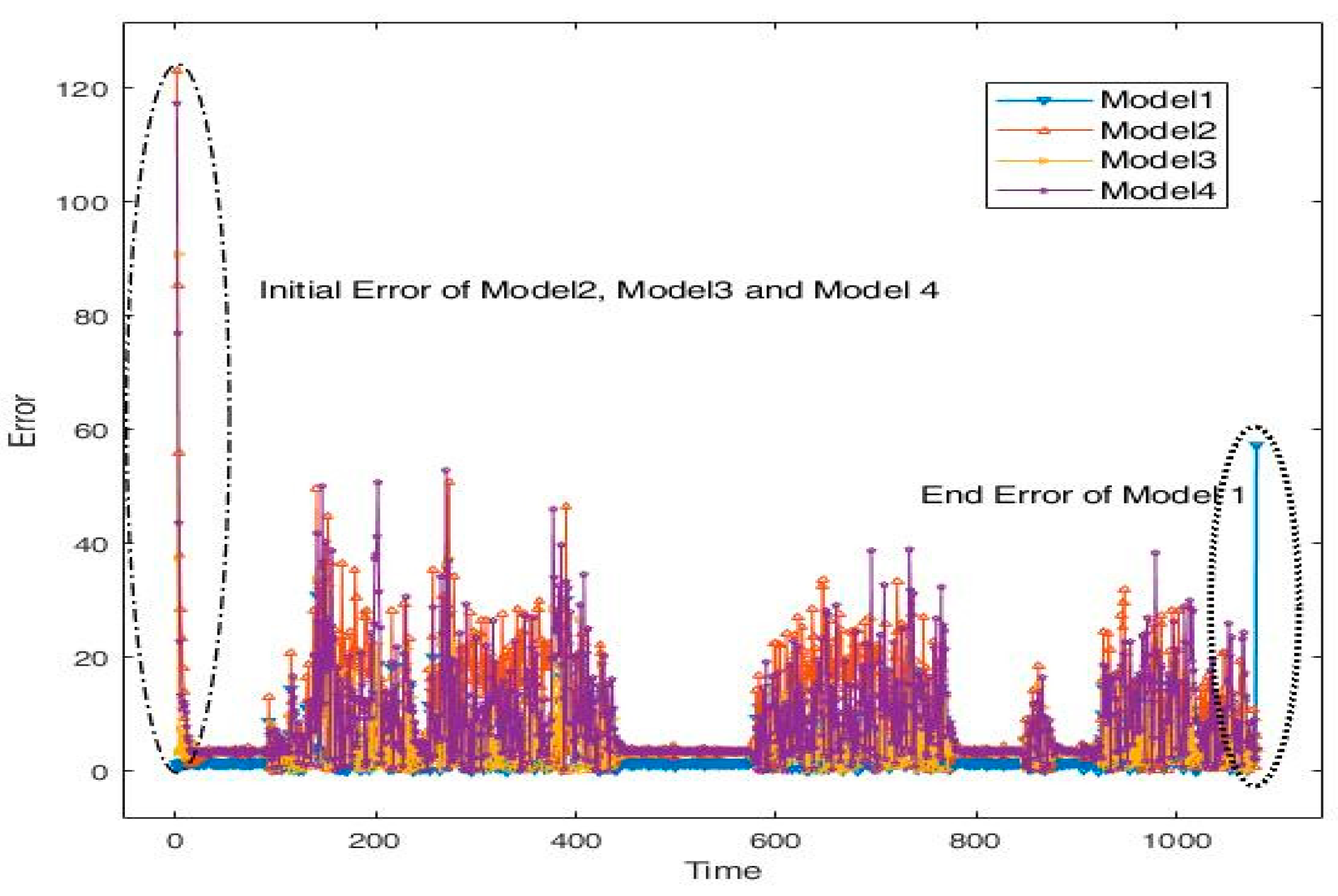
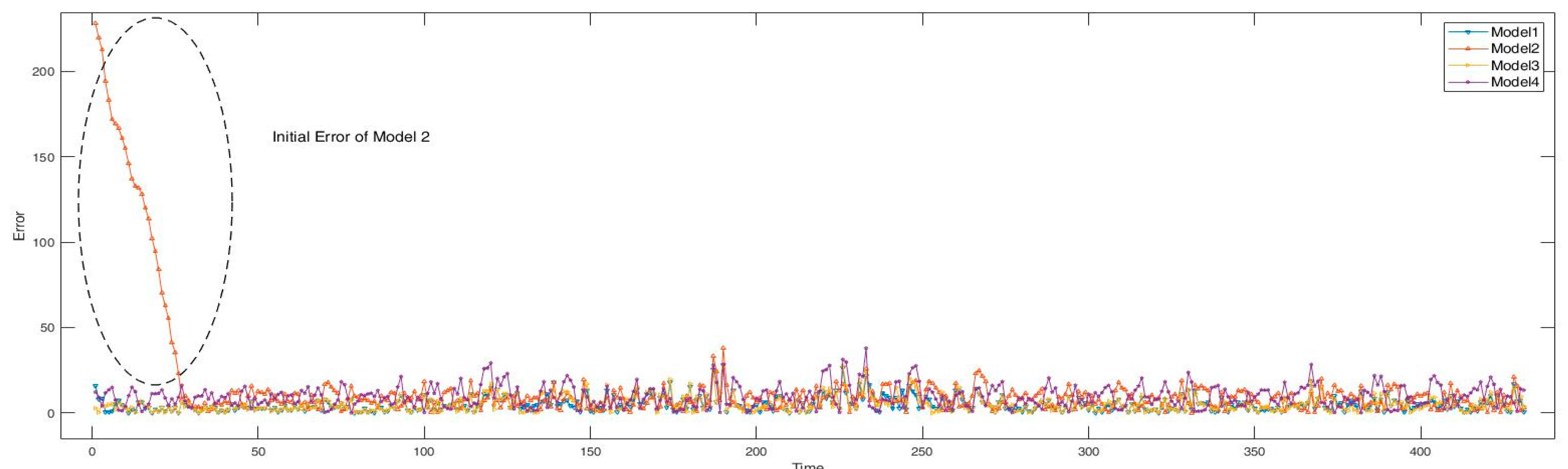
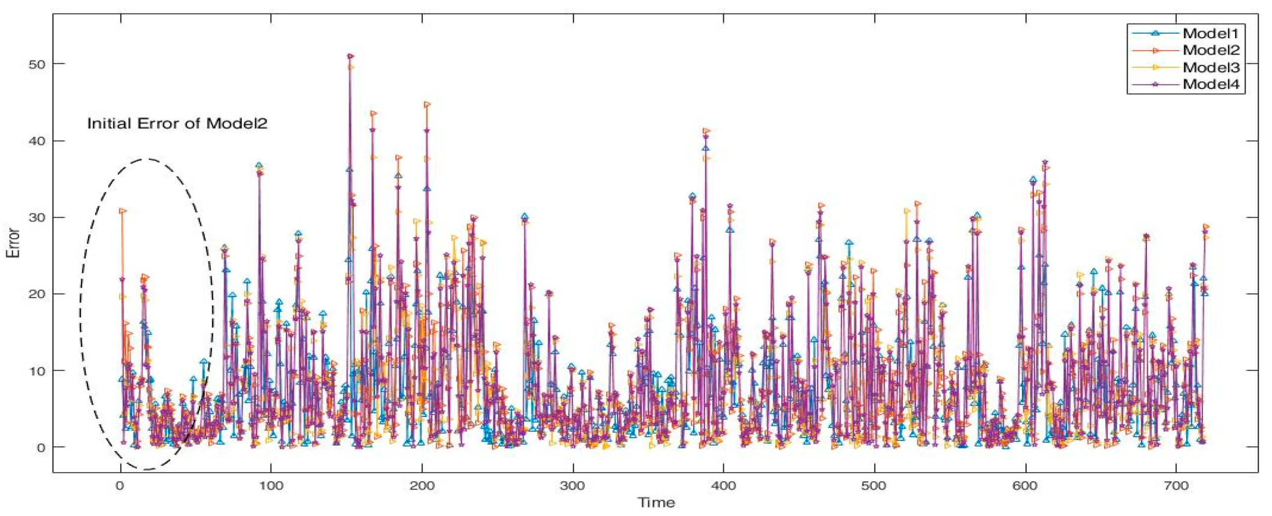
Figure 6, Figure 7 and Figure 8 show the results of applying the modified LSTM to models in A, B, and C regions of Jeju Island. The prediction error is the difference between the observed value and the proposed value for each model. Experimental results show that the prediction of M1 was superior in the early stage, but the performance drastically decreased due to error accumulation in the tail. On the other hand, predictions of M2, M3, and M4 showed poor performance at the beginning, but they improved towards the latter half. The reason why wind power adopted by M1 is the smallest at initial error is because of the high volatility, which the shorter the collected data time, the more efficient short-term wind power prediction. The correlation between wind power and wind speed adopted by M3 is high. That is, the higher the wind power, the larger the wind speed.
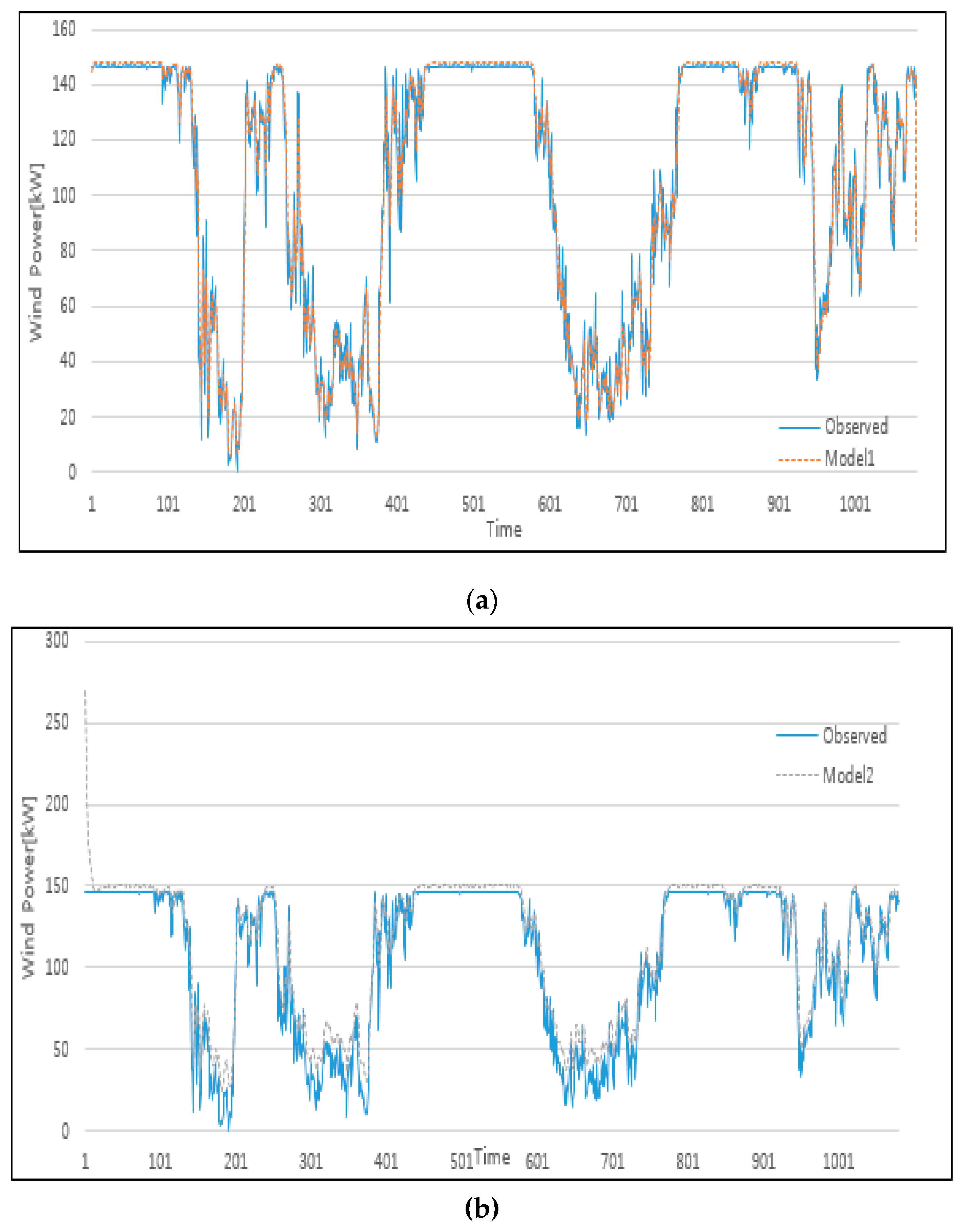
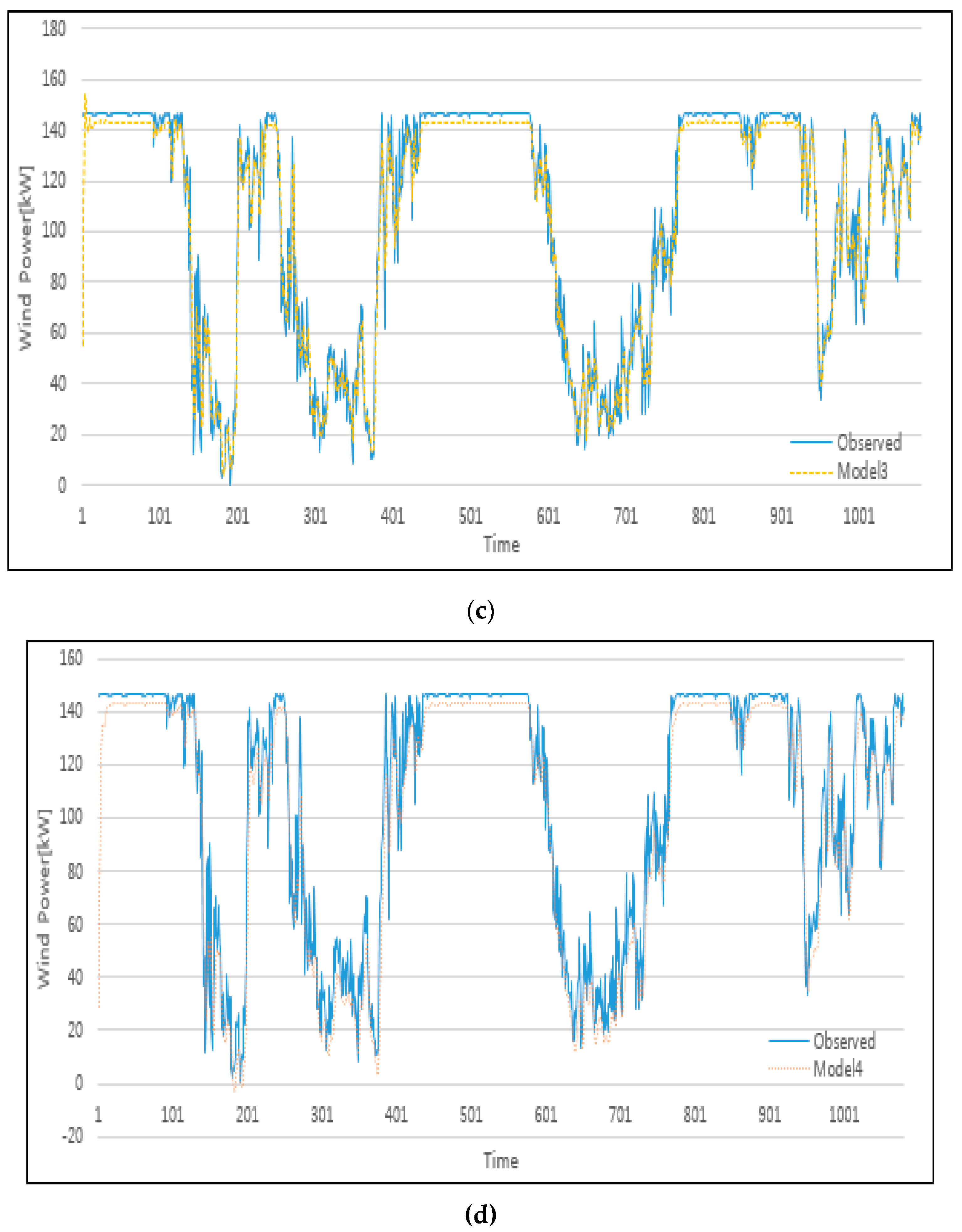
Figure 9 shows the comparison of wind power prediction by models using the modified LSTM in A region of Jeju Island. Figure 9a shows that the predicted value was similar to the measured value at the beginning, but the predicted value deviated from the observed value towards the middle. Figure 9b shows that the predicted value was higher than the observed value initially, but the predicted value was similar to the observed value towards the middle. Finally Figure 9c,d show that the predicted value was lower than the observed value at the beginning, but the predicted and observed values became similar from the mid-point.
4.4. Comparison and Analysis of Hybrid Forecasting Model
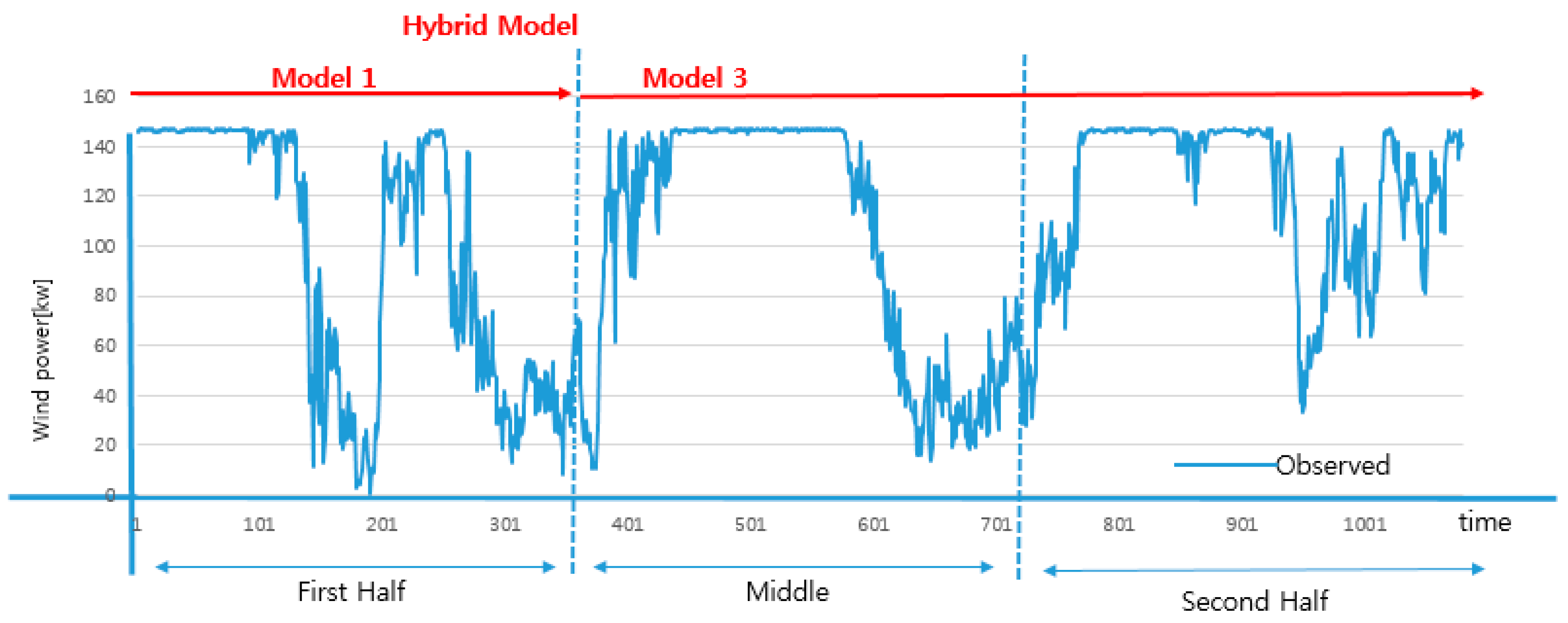
We propose a hybrid forecasting model that combines M1 and M3 with the least prediction error for each model mentioned in the previous Section 4.3. That is, M1 has the smallest initial error and M3 has the smallest error from the middle to the end. This is because wind power has the greatest impact on short-term wind power forecasts, followed by wind power and wind speed. As shown in Figure 10, in the learning and testing of the proposed hybrid forecasting model, M1 is used at the beginning (first half), and M3 is applied from the middle to the end according to time.
Table 5 presents the error metrics of wind power prediction by using the hybrid model, and Table 6 shows the performance analysis of the hybrid model with other models in A, B, and C regions of Jeju Island. In Table 6, △M1, △M2, △M3, and △M4 are the difference between each model, and the hybrid model and superior values are shaded. It is noteworthy that the improvement degrees on the hybrid model are obviously larger than on other models. On average, RMSE, MAPE, and complex time of the three regions are as follows: (1) regarding RMSE, the proposed hybrid model showed improvement degrees at −3.6, −16.0, −4.6, and −7.7, respectively, as compared with the other models. (2) Regarding MAPE, the proposed method showed superior error reduction at −6.7%, −28.0%, −7.6%, and −17.8%, respectively. (3) Regarding complex time, the proposed method showed superior time reduction over all other models, except for M1. Therefore, M2 and M4 using wind direction were found to not affect wind power prediction.
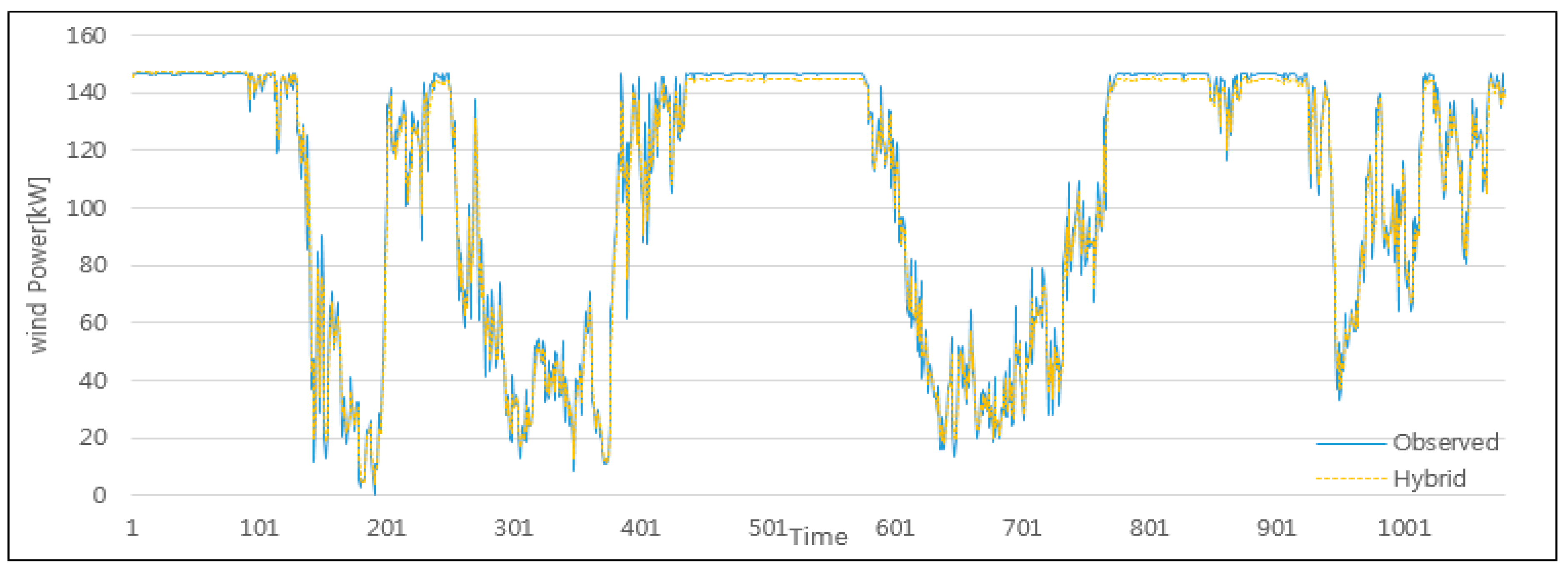
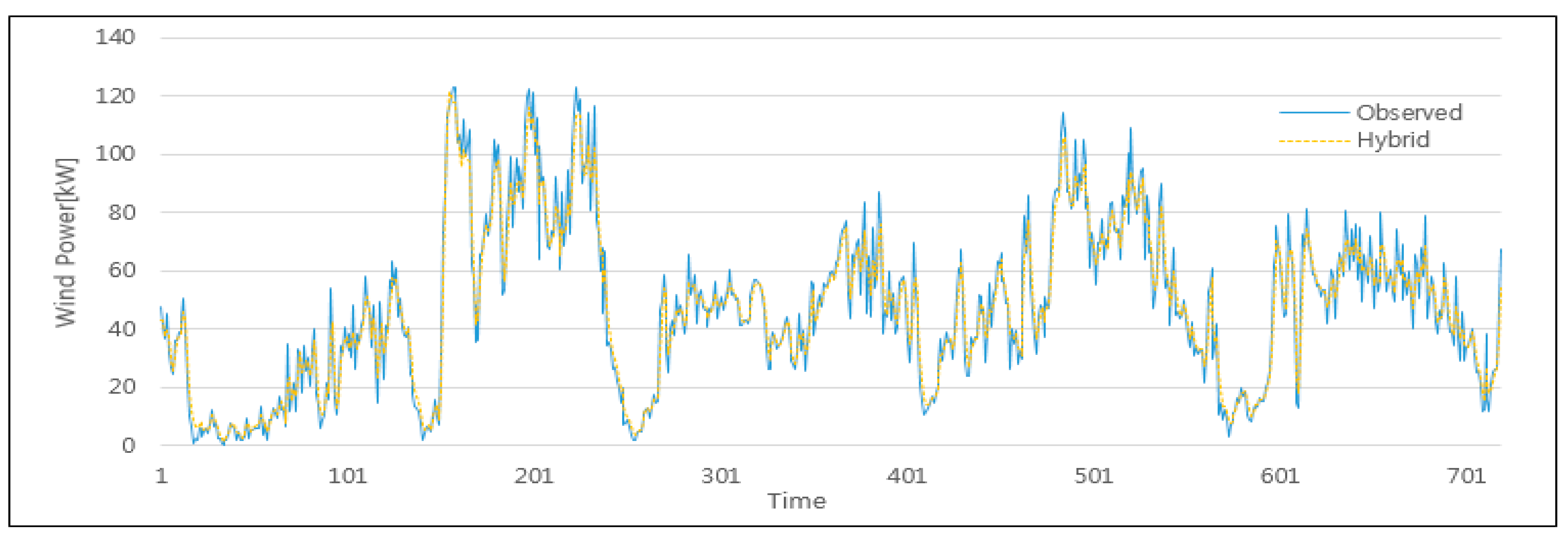
Figure 11, Figure 12 and Figure 13 depict the wind power prediction results of the hybrid model with M1 and M3. As shown in the simulation results, the wind speed was predicted well in the early and late parts without errors. Therefore, it is verified that the proposed hybrid forecasting model is effective at improving the performance of wind power prediction.
5. Conclusions
Recently, LSTM has been used extensively in time series analysis because of its superior deep learning performance among artificial intelligence methods. Although it has excellent performance in terms of versatility, it has a disadvantage in that it cannot explain the causal relationship between predictive factors affecting short-term wind power. Therefore, in this study, four models were set using LSTM, which is a deep learning, and the causality between wind power, wind direction, and wind speed was tested. After analyzing the advantage and disadvantage of the four models, we proposed a hybrid model. The experiment results showed that the proposed method can realize a short-term wind power prediction system suitable for the specific characteristics of the weather and topography in areas where wind power equipment is installed, and it can be expected to reduce the production cost of domestic electric energy. Future studies are as follows: (1) We will compare the performance of the proposed method with that of the existing methods (ARIMA, persistence models, SVM, etc.) (2) We will extend the study to domestic and overseas wind power complexes. (3) Experiments will be conducted to the forecast of mid- to long-term wind power.
Author Contributions
All authors contributed to this research. N.S. implemented the algorithm for theory and writing. S.Y. collected the data set and performed the analysis. J.N. supported the theorizing and review and editing.
Funding
This article was supported by Korea Energy Technology Evaluation & Planning under the financial resources of the government in 2018 (20182410105210, Development and demonstration of multi-use application technology of consumer ESS).
Conflicts of Interest
The authors declare no conflict of interest.
References
- Woori Finance Research Institute. Recent Trends in Renewable Energy Industry; Woori Finance Research Institute: Seoul, Korea, 2019. [Google Scholar]
- Seo, I.Y.; Ha, B.N.; Kim, S.O.; Koong, W.N.; Seo, D.W.; Kim, S.J. Short term wind power prediction using wavelet transform and ARIMA. J. Energy Power Eng. 2012, 6, 1786–1790. [Google Scholar]
- Hong, Y.Y.; Yu, T.H.; Liu, C.Y. Hour-Ahead wind speed and power forecasting using empirical mode decomposition. Energies 2013, 6, 6137–6152. [Google Scholar] [CrossRef]
- Noh, C.H.; Jang, W.H.; Kim, C.H. Recent Trends in Renewable energy Resources for Power Generation in the Republic of Korea. Resources 2015, 4, 751–764. [Google Scholar] [CrossRef]
- Okumus, I.; Dinler, A. Current status of wind energy forecasting and a hybrid method for hourly predictions. Energy Convers. Manage. 2016, 123, 362–371. [Google Scholar] [CrossRef]
- Sarwat, A.; Amini, M.; Domijan, A.; Damnjanovic, A.; Kaleem, F. Weather-based interruption prediction in the smart grid utilizing chronological data. J. Mod. Power Syst. Clean Energy 2016, 4, 308–315. [Google Scholar] [CrossRef]
- Chen, N.; Qian, Z.; Nabney, I.T.; Meng, X. Wind power forecasts using Gaussian processes and numerical weather prediction. IEEE Trans. Power Syst. 2014, 29, 656–665. [Google Scholar] [CrossRef]
- Jiang, Y.; Chen, X.; Yu, K.; Liao, Y. Short-term wind power forecasting using hybrid method based on enhanced boosting algorithm. J. M. Power Syst. Clean Energy 2015, 5, 126–133. [Google Scholar] [CrossRef] [Green Version]
- Fathall, A.; Timothy, M.; Siddharth, S.; Edwin, K.P. Employing ARIMA models to improve wind power forecasts: A case study in ERCOT. In Proceedings of the 2016 North American Power Symposium (NAPS), Denver, CO, USA, 18–20 September 2016. [Google Scholar]
- Nury, A.H.; Hasan, K.; Alam, M.J.B. Comparative Study of Wavelet-ARIMA and Wavelet-ANN Models for Temperature Time Series Data in Northeastern Bangladesh. J. King Saud Univ.-Sci. 2017, 29, 47–61. [Google Scholar] [CrossRef]
- Khodayar, M.; Wang, J.; Manthouri, M. Interval Deep Generative Neural Network for Wind Speed Forecasting. IEEE Trans. Smart Grid 2019, 10, 3974–3989. [Google Scholar] [CrossRef]
- Kassa, Y.; Zhang, J.H.; Zheng, D.H.; Wei, D. Short term wind power prediction using ANFIS. In Proceedings of the IEEE International Conference on Power and Renewable Energy (ICPRE), Shanghai, China, 21–23 October 2016. [Google Scholar]
- Wang, J.; Fang, K.; Pang, W.; Sun, J. Wind power interval prediction based on improved PSO and BO neural network. J. Electr. Eng. Tech. 2017, 12, 989–995. [Google Scholar] [CrossRef]
- Suhan, Z. Wind Power Prediction Based on Genetic Neural Network, AIP Conference Proceedings 1834; AIP Publishing: Melville, NY, USA, 2017. [Google Scholar]
- Mariya, S.; Ilya, K.; Thorsten, S. Supervised Classification with Interdependent Variable to Support Targeted Energy Efficiency Measures in the Residential Sector. Decis. Analytics 2016, 3, 1. [Google Scholar]
- Renani, E.; Elias, M.; Rahim, N.A. Using Data-driven Approach for Wind Power Prediction: A Comparative Study. Energy Convers. Manag. 2016, 118, 193–203. [Google Scholar] [CrossRef]
- Ministry of Trade, Industry and Energy. An Empirical Study for 2.5GW Offshore Wind Power in the Southwest Sea; Ministry of Trade, Industry and Energy: Sejong City, Korea, 2014.
- Kim, H.G.; Lee, Y.S.; Jang, M.S. Cluster Analysis and Meteor-Statistical Model Test to Develop a Daily Forecasting Model for Jejudo Wind Power Generation. J. Environ. Sci. Int. 2010, 19, 1229–1235. [Google Scholar] [CrossRef]
- Botterud, A.; Miranda, V.; Wang, J.; Monteiro, C. Wind Power Forecasting and Electricity Market Operations. In Proceedings of the CPES Annual Conference, Blacksburg, VA, USA, 5–7 April 2009. [Google Scholar]
- Zack, J.W. Overviw of the Current Status and Future Prospects of Wind Power Production Forecasting for the ERCOT System. In Proceedings of the Wind Workshop III ERCOT Workshop, Austin, TX, USA, 26 June 2009. [Google Scholar]
- Cellura, M.; Cirrincione, G.; Marvuglia, A.; Miraoui, A. Wind Speed Spatial Estimation for Energy Planning in Sicily: Introduction and Statistical Analysis. Renew. Energy 2008, 33, 1237–1250. [Google Scholar] [CrossRef]
- Wang, J.; Liu, L.D.; Wang, Z.Y. The Status and Development of the Combination Forecast Method. Forecast 1997, 6, 37–45. [Google Scholar]
- Lei, M.; Shiyan, L.; Chuanwen, J.; Hongling, L.; Yan, Z. A Review on the Forecasting of Wind Speed and Generated Power. Renew. Sustain. Energy Rev. 2009, 13, 15–35. [Google Scholar] [CrossRef]
- Esen, H.; Inalli, M.; Sengur, A.; Esen, M. Modeling a Ground-coupled Heat Pump System by a Support Vector Machine. Renew. Energy 2008, 33, 1814–1837. [Google Scholar] [CrossRef]
- Chen, H. The Validity of the Theory and its Application of Combination Forecast Methods; Beijing Science Press: Beijing, China, 2008. [Google Scholar]
- Zhao, W.; Wang, J.; Lu, H. Combining Forecasts of Electricity Consumption in China with Time-varying Weights Updated by a High-order Markov Chain. Omega 2014, 45, 80–91. [Google Scholar] [CrossRef]
- Tascikaraoglu, A.; Uzunoglu, M. A Review of Combined Approaches for Prediction of Short-term Wind Speed and Power. Renew. Sustain. Energy Rev. 2014, 34, 243–254. [Google Scholar] [CrossRef]
- Bouzgou, H.; Benoudjit, N. Multiple Architecture System for Wind Speed Prediction. Appl. Energy 2011, 88, 2463–2471. [Google Scholar] [CrossRef]
- Lei, C.; Ran, L. Short-term Wind Speed Forecasting Model for Wind Farm based on Wavelet Decomposition. In Proceedings of the Third International Conference on Electric Utility Deregulation and Restructuring and Power Technologies (DRPT), Nanjing, China, 6–9 April 2008; pp. 2525–2529. [Google Scholar]
- Guo, Z.; Zhao, W.; Lu, H.; Wang, J. Multi-step Forecasting for Wind Speed using a Modified EMD-based Artificial Neural Network Model. Renew. Energy 2012, 37, 241–249. [Google Scholar] [CrossRef]
- Zhou, H.; Jiang, J.; Huang, M. Short-term Wind Power Prediction based on Statistical Clustering. In Proceedings of the IEEE Power and Energy Society General Meeting, Detroit, MI, USA, 24–28 July 2011; pp. 1–7. [Google Scholar]
- Kani, S.P.; Ardehali, M.M. Very Short-term Wind Speed Prediction: A New Artificial Neural Network-Markov Chain Model. Energy Convers. Manag. 2011, 52, 738–745. [Google Scholar] [CrossRef]
- Li, X.; Liu, Y.; Xin, W. Wind Speed Prediction based on Genetic Neural Network. In Proceedings of the 4th IEEE Conference on Industrial Electronics and Applications, Xi’an, China, 25–27 May 2009; pp. 2448–2451. [Google Scholar]
- Su, Z.; Wang, J.; Lu, H.; Zhao, G. A New Hybrid Model Optimized by an Intelligent Optimization Algorithm for Wind Speed Forecasting. Energy Convers. Manag. 2014, 85, 443–452. [Google Scholar] [CrossRef]
- Hui, T.; Niu, D. Combining Simulate Anneal Algorithm with Support Vector Regression to Forecast Wind Speed. In Proceedings of the Second IITA International Conference on Geoscience and Remote Sensing (IITA-GRS), Qingdao, China, 28–31 August 2010; pp. 92–94. [Google Scholar]
- Qu, X.; Kang, X.; Zhang, C.; Jiang, S.; Ma, X. Short-term Prediction of Wind Power based on Deep Long Short-term Memory. In Proceedings of the 2016 IEEE PES Asia-Pacific IEEE, Power and Energy Engineering Conference (APPEEC), Xi’an, China, 25–28 October 2016; pp. 1148–1152. [Google Scholar]
- Louka, P.; Galanis, G.; Siebert, N.; Kariniotakis, G.; Katsafados, P.; Pytharoulis, I. Improvements in Wind Speed Forecasts for Wind Power Prediction Purposes using Kalman Filtering. J. Wind Eng. Ind. Aerodyn. 2008, 96, 2348–2362. [Google Scholar] [CrossRef]
- Hochreiter, S.; Schmidhuber, J. LSTM can Solve Hard Long Time Lag Problems. In Proceedings of the Advances in Neural Information Processing Systems, Denver, CO, USA, 2–5 December 1996; pp. 473–479. [Google Scholar]
- Patterson, J.; Gibson, A. Deep Learning. A Practitioner’s Approach; O’Reilly Media, Inc.: Sebastopol, CA, USA, 2017; pp. 150–158. [Google Scholar]
- Colah.github.io. Understanding LSTM Networks—Colah’s Blog. Available online: http://colah.github.io/posts/2015-08-Understanding-LSTMs (accessed on 12 October 2019).
- Negnevitsky, M.; Potter, C.W. Innovative short-term wind generation prediction techniques. IEEE Power Syst. Conf. Expo. 2006, 60–65. [Google Scholar]
- Foley, A.M.; Leahy, P.G.; Marvuglia, A.; McKeogh, E.J. Current methods and advances in forecasting of wind power generation. Renew. Energy 2012, 37, 1–8. [Google Scholar] [CrossRef] [Green Version]
- Lee, Y.S.; Kim, J.; Jang, M.S.; Kim, H.G. A study on comparing short-term wind power prediction models in Gunsan wind farm. J. Korean Data Inf. Sci. Soc. 2013, 24, 585–592. [Google Scholar]
- Computation Time. Available online: http://mathworld.wolfram.com/ComputationTime.html (accessed on 12 October 2019).
Figure 1.
Recurrent Neural Network and unfolding during computation time.

Figure 2.
Structure of long short-term memory.

Figure 3.
Flowchart of the proposed approach.

Figure 4.
Wind power prediction of existing long short-term memory (LSTM): (a) Comparison of observed values with predicted values using LSTM; (b) Predicted error for observed values and predicted values.
Figure 4.
Wind power prediction of existing long short-term memory (LSTM): (a) Comparison of observed values with predicted values using LSTM; (b) Predicted error for observed values and predicted values.

Figure 5.
Wind power prediction of the modified long short-term memory (LSTM): (a) Comparison of observed values with predicted values using LSTM; (b) Predicted error for observed values and predicted values.
Figure 5.
Wind power prediction of the modified long short-term memory (LSTM): (a) Comparison of observed values with predicted values using LSTM; (b) Predicted error for observed values and predicted values.

Figure 6.
Comparison of predictive errors for each model in A region of Jeju Island.

Figure 7.
Comparison of predictive errors for each Model in B region of Jeju Island.

Figure 8.
Comparison of predictive errors for each model in C region of Jeju Island.

Figure 9.
Comparison of wind power prediction by models using the proposed long short-term memory in A region of Jeju Island: (a) Comparison of observed value with Model 1; (b) Comparison of observed value with Model 2; (c) Comparison of observed value with Model 3; (d) Comparison of observed value with Model 4.


Figure 10.
Wind power prediction by using the hybrid model.

Figure 11.
Comparisons between the observation and hybrid model in A region of Jeju Island.

Figure 12.
Comparisons between the observation and hybrid model in B region of Jeju Island.

Figure 13.
Comparisons between the observation and hybrid model in C region of Jeju Island.


Table 1.
Collection period, collection time, learning and testing data of each region.
| Region | Collection Period | Collection Time | Learning Data | Test Data | Total Data |
|---|---|---|---|---|---|
| A | 2014.01.11–25 | 10 min | 1080 | 1080 | 2160 |
| B | 2014.01.11–20 | 10 min | 1008 | 432 | 1440 |
| C | 2014.01.11–25 | 10 min | 1440 | 720 | 2160 |
Table 2.
Information about wind turbine generators in A, B, and C regions of Jeju Island.
| Area | A | B | C | |
|---|---|---|---|---|
| Specifications | ||||
| Model | U88 | U50 | ||
| Output | 2000 kW | 750 kW | ||
| Wind speed | 12 m/s | 12.5 m/s | ||
| Rotor speed range | 6–17.5 rpm | 9–28 rpm | ||
| Voltage and frequency | 690V/60 Hz | 690V/60 Hz | ||
| Rotor diameter | 88 m | 50 m | ||
| Hub height | 80 m | 50 m | ||
| Power control | Pitch | Pitch | ||
Table 3.
Multivariate Models.
| Model | Variables |
|---|---|
| Model 1 (M1) | wind power |
| Model 2 (M2) | wind power, wind direction |
| Model 3 (M3) | wind power, wind speed |
| Model 4 (M4) | wind power, wind direction, wind speed |
Table 4.
Comparison of results obtained using Models in A, B, and C Regions of Jeju Island.
| Region | RMSE | MAPE (%) | Complex Time (s) | |||||||||
|---|---|---|---|---|---|---|---|---|---|---|---|---|
| M1 | M2 | M3 | M4 | M1 | M2 | M3 | M4 | M1 | M2 | M3 | M4 | |
| A | 6.3 | 13.2 | 8.1 | 12.7 | 7.9 | 28.0 | 10.5 | 14.0 | 36.6 | 65.8 | 65.2 | 94.5 |
| B | 6.7 | 35.8 | 6.9 | 11.5 | 5.1 | 41.9 | 3.1 | 30.2 | 32.1 | 57.0 | 55.1 | 78.2 |
| C | 10.6 | 11.8 | 11.4 | 11.6 | 32.6 | 39.5 | 34.8 | 34.7 | 26.3 | 47.0 | 45.3 | 64.4 |
Table 5.
Error metrics of the hybrid forecasting model in A, B, and C regions of Jeju Island.
| Region | RMSE | MAPE (%) | Complex Time (s) |
|---|---|---|---|
| A | 3.67 | 5.04 | 45.18 |
| B | 3.39 | 3.36 | 39.20 |
| C | 5.64 | 17.09 | 32.11 |
Table 6.
Performance analysis of the hybrid model with other models.
| Region | RMSE | MAPE (%) | Complex Time (s) | |||||||||
|---|---|---|---|---|---|---|---|---|---|---|---|---|
| △M1 | △M2 | △M3 | △M4 | △M1 | △M2 | △M3 | △M4 | △M1 | △M2 | △M3 | △M4 | |
| A | −2.6 | −9.5 | −4.4 | −9.0 | −2.8 | −22.9 | −5.4 | −8.9 | 8.5 | −20.6 | −20.0 | −49.3 |
| B | −3.3 | −32.4 | −3.5 | −8.1 | −1.7 | −38.5 | 0.2 | −26.8 | 7.1 | −17.8 | −15.9 | −39.0 |
| C | −4.9 | −6.1 | −5.7 | −5.9 | −15.5 | −22.4 | −17.7 | −17.6 | 5.8 | −14.8 | −13.1 | −32.2 |
| Avg. | −3.6 | −16.0 | −4.6 | −7.7 | −6.7 | −28.0 | −7.6 | −17.8 | 7.2 | −17.8 | −16.4 | −40.2 |
© 2019 by the authors. Licensee MDPI, Basel, Switzerland. This article is an open access article distributed under the terms and conditions of the Creative Commons Attribution (CC BY) license (http://creativecommons.org/licenses/by/4.0/).
Share and Cite
MDPI and ACS Style
Son, N.; Yang, S.; Na, J. Hybrid Forecasting Model for Short-Term Wind Power Prediction Using Modified Long Short-Term Memory. Energies 2019, 12, 3901. https://doi.org/10.3390/en12203901
AMA Style
Son N, Yang S, Na J. Hybrid Forecasting Model for Short-Term Wind Power Prediction Using Modified Long Short-Term Memory. Energies. 2019; 12(20):3901. https://doi.org/10.3390/en12203901
Chicago/Turabian StyleSon, Namrye, Seunghak Yang, and Jeongseung Na. 2019. "Hybrid Forecasting Model for Short-Term Wind Power Prediction Using Modified Long Short-Term Memory" Energies 12, no. 20: 3901. https://doi.org/10.3390/en12203901
Note that from the first issue of 2016, this journal uses article numbers instead of page numbers. See further details here.