A Review on Time Series Aggregation Methods for Energy System Models


1
Institute of Energy and Climate Research, Techno-economic Systems Analysis (IEK-3), Forschungszentrum Jülich, 52428 Jülich, Germany
2
Chair for Fuel Cells, RWTH Aachen University, c/o Institute of Electrochemical Process Engineering (IEK-3), Forschungszentrum Jülich GmbH, Wilhelm-Johnen-Str., 52428 Jülich, Germany
*
Author to whom correspondence should be addressed.
Energies 2020, 13(3), 641; https://doi.org/10.3390/en13030641
Submission received: 6 November 2019
/
Revised: 9 January 2020
/
Accepted: 13 January 2020
/
Published: 3 February 2020
(This article belongs to the Special Issue Clustering of the Electricity Consumption Time Series in the Big Data Era)
Abstract
:Due to the high degree of intermittency of renewable energy sources (RES) and the growing interdependences amongst formerly separated energy pathways, the modeling of adequate energy systems is crucial to evaluate existing energy systems and to forecast viable future ones. However, this corresponds to the rising complexity of energy system models (ESMs) and often results in computationally intractable programs. To overcome this problem, time series aggregation (TSA) is frequently used to reduce ESM complexity. As these methods aim at the reduction of input data and preserving the main information about the time series, but are not based on mathematically equivalent transformations, the performance of each method depends on the justifiability of its assumptions. This review systematically categorizes the TSA methods applied in 130 different publications to highlight the underlying assumptions and to evaluate the impact of these on the respective case studies. Moreover, the review analyzes current trends in TSA and formulates subjects for future research. This analysis reveals that the future of TSA is clearly feature-based including clustering and other machine learning techniques which are capable of dealing with the growing amount of input data for ESMs. Further, a growing number of publications focus on bounding the TSA induced error of the ESM optimization result. Thus, this study can be used as both an introduction to the topic and for revealing remaining research gaps.
1. Introduction
1.1. Drivers of Model Complexity
Due to the climate change caused by anthropogenic CO2 emissions resulting from the burning of fossil fuels, a major turnaround in the fields of energy supply and consumption is an increasing necessity. Key aspects of addressing this challenge are the integration of renewable energy sources (RES) into existing energy systems, as well as a closer coupling of energy forms and sectors [1].
The evolution of the energy sector has been accompanied by a consistent effort to model and predict its development. Early attempts to forecast future energy demands can be traced back to the 1950s and constitute simple, assumption-based scenarios [2]. Another theoretical foundation for modern energy system models (ESMs) is the principle of peak-load-pricing first described by Boiteux in 1949 [3] (English translation in 1960 [4]) and Steiner in 1957 [5]. This approach distinguishes between capacity and the operating costs of facilities producing non-storable goods. Thus, it applies to many simple energy systems with a single good (commodity), e.g., electricity which has led to the development of approaches to solve simple generation expansion planning (GEP) problems with the annual load duration curve as shown by Sherali et al. [6]. As key drivers for the early progress of energy system modelling, three factors are of particular significance:
Ever since the first ESMs, based on optimizations rather than just simulations, were developed during the 1970s and 1980s [9,11], two major options arose for their developers, namely whether to focus on economic mechanisms, sometimes described as a top-down approach, or on the technical dimension, usually known as a bottom-up one [12,13]. Amongst the bottom-up frameworks, this review focuses on a vast number of approaches to modeling the different dimensions of energy systems, including methodologies such as optimizations and simulations [9,12,13]. With respect to the scope of ESMs, two fundamental dimensions can be delineated: namely spatiotemporal and techno-economic. The spatiotemporal dimension comprises the setting of input data that a model is intended to incorporate. The spatial sub-dimension is focused on the number of regions and their connections to each other, as energy systems on a national or even larger scale usually face the challenge of taking energy transmission between different regions into account. The temporal sub-dimension is divided into two aspects, namely temporal resolution (TR), often referred to as time steps, and the overall time horizon [9], which also concerns questions of storage modeling [14,15,16,17,18,19,20] as well as the linking of dynamic processes [21,22,23] and investment dynamics [24,25]. In contrast, the techno-economic dimension deals with how the components are represented in the model and whether their design and/or operation are optimized or, if their operational behavior is simply simulated, how they are mathematically represented and if the impact of supply and demand on energy prices is dynamically modeled or not [13]. Each of the dimensions listed above drives the overall complexity of ESMs, while the spatiotemporal resolution also affects the techno-economical dimension directly, e.g., the TR also limits the (technical) operational exactness of components in the energy system.
1.2. Motivation and Scope of the Review
Although Moore’s law has held true for approximately 40 years [31,32] and there have been significant advances made in the branch-and-bound algorithms used for solving big mixed integer linear programs (MILPs) such as those used in energy system optimization models [33], a decelerating increase of transistor density could be observed in recent years [34]. On the other hand, liberalization, decentralization, and an increasing volatility in energy generation [35] are leading to more complex applications for ESMs. Therefore, the recent number of publications dealing with aggregation methods in ESMs illustrates the fact that many application cases are too complex to be overcome solely by computational power and mathematically equivalent transformations.
As mentioned above, the temporal sub-dimension in ESMs is crucial for the implementation of storages and the description of system dynamics, which is especially important for ESMs considering a high share of intermittent RES [36,37,38,39,40,41]. This applies for both single-node and multi-node ESMs, and the group of aggregation methods employed to tackle this issue is broad and diverse. Hence, this review addresses the issue of systematically categorizing the methods and their assumptions, as well as recent trends and the general shortcomings in the development of TSA methods. Furthermore, this work is intended to facilitate the development of new methods by combining existing methods and considering the shortcomings present. This endeavor differs from the scope of recent publications focusing on the general purpose of TSA [42]. The temporal sub-dimension that the aggregation methods presented in the following address is highlighted in Figure 1. As the input time series for constrained bottom-up ESM are often not only auto-correlated, i.e., to some extent periodic, but also cross-correlated, an aggregation based on time series can be applied in multiple ways. This review focuses only on the aggregation of time series based on their auto-correlation, i.e., the reduction of the number of time steps, e.g., by representing a whole year of data by a small number of typical days. This is represented by the rotating arrow in Figure 1 and will be defined as TSA in the narrow sense. In contrast, a reduction of the number of regions, technologies, or customer profiles is based on the mutual similarity of the same attributes at different locations or different attributes at the same location. Therefore, spatial or technological aggregation approaches are reducing the number of time series, but not the number of time steps.
2. Methodology and Structure of the Review
As highlighted above, this review focuses on the TSA methods in bottom-up energy system optimization models that include generation expansion planning (GEP), as well as unit commitment (UC) and have constantly emerged and evolved since the late 1970s and 1980s [9,11]. Among the early model frameworks, one group focuses on long-term system planning and has usually only one time step per year such as LEAP [43], EFOM [44], and BESOM [45], which are not subject to aggregation techniques and thus neglected in the following. The temporal dimension of the other major group of early bottom-up ESMs such as TIMES [46,47,48,49] and its predecessors MARKAL [50], MESSAGE [12,51], IKARUS [9], and PERSEUS [52] are based on time slice formulations (in the case of PERSEUS called “time slots”), which are explained in more detail in Section 3.2.1. Although the long-term planning models with only one time step per year were consecutively combined with models with a higher temporal resolution, as is the case for TIMES [46,47,48,49] as a combination of MARKAL [50] and EFOM [44], the time slice approach, which is based on the modeler’s experience only, remained unchanged for decades. With the first approaches to classify and group demand curves using unsupervised learning techniques, which the authors traced back to 1999 [53], new techniques for defining the temporal dimension of ESMs arose. To the best of the authors’ knowledge, this was first done manually in 2008 [54] and by using a standard clustering algorithm in 2011 [55]. In order to investigate the rapid and manifold development of complex TSA methods based on feature-based grouping in detail, the start year for the literature review was set to 1999 and the literature research was stopped in July 2019. To avoid a bias towards the new methods based on unsupervised learning techniques, publications within the relevant time interval, which are based on long-existing and constantly evolving frameworks such as TIMES, are also considered. Thus, the research objective is narrowly defined and can be exhaustively examined.
2.1. Methodology of the Literature Research
With respect to a systematic and keyword-based search for TSA methods, the major challenge was the inconsistent naming of the applied methods. Furthermore, the majority of publications did not explicitly address the comparison of the different aggregation methods. Instead, the TSA methods were often simply applied. Therefore, terms such as TSA, TD, complexity reduction, or clustering, which are crucial for identifying TSA methods, only appear in a minority of publications as keywords. Moreover, a number of terms was found to be inconsistently or redundantly used by different research communities. Examples for this are the terms “representative days” and “typical days”. Therefore, a heuristic approach was used as starting point that focused on a search for methods based on citations of earlier works. If no earlier work was cited dealing with TSA, the search was halted. Simultaneously, terms that appeared in multiple publications were considered to be keywords and, to overcome the problem of co-citation clusters [56] with own terms, these newly defined keywords were used for an additional search on the internet. The keywords used for the literature research that arose from this analysis are listed in Table 1 along with their definitions and terms that are synonymously used in the literature.
Building upon the analyzed literature and the basic features of a TSA process introduced by Kotzur et al. [57] and Schütz et al. [58], the table of methods in Appendix A was derived for categorizing and comparing the different methods. Moreover, the methods were also investigated on the basis of their capacity to link all time steps across the original time horizon, which enables seasonal storage, and their premise to approximate the duration curve or the unsorted time series. This ultimately leads to the structure of the following sections.
2.2. Structure of the Review
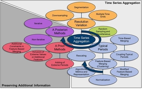
From the categorization in Appendix A, the methods presented in Section 3 are derived as the basic aggregation methods, as well as miscellaneous methods that cannot be clearly categorized. As aggregation methods commonly suffer from certain drawbacks, a number of methods exist to preserve additional information of the original input time series, which are presented in Section 4. Along with both Section 3 and Section 4, the individual trends and possible reasons for them are discussed in Section 3.5 and Section 4.3. The major results of the review are concluded in Section 5.
Figure 2 illustrates the structure of the following chapters by highlighting comparable ideas with rival methods with the same colors and steps to be taken or decisions to be made for applying a sophisticated aggregation method with blue arrows. The grey backgrounds distinguish the basic aggregation process presented in Section 3 from the preservation of additional information of the original time series presented in Section 4.
Along with the introduction of a new aggregation method, the impact of this method on potential input data is visualized. For this, a time series for photovoltaic capacity factors is used, which consists of 8760 hourly time steps for one year, and is illustrated in Figure 3. Finally, all of the described equations refer to those in existing publications, but are reformulated for the sake of consistency within this paper.
3. Time Series Aggregation
The following section deals with the general concept of TSA. For the mathematical examinations of the following section, the nomenclature of Table 2 is used.
The input data usually consists of one time series for each attribute, i.e., . The set of attributes describes all types of parameters that are ex-ante known for the energy system, such as the capacity factors of certain technologies at certain locations or demands for heat and electricity that must be satisfied. The set of time steps describes the shape of the time series itself, i.e., sets of discrete values that represent finite time intervals, e.g., 8760 time steps of hourly data to describe a year. For all methods presented in the following, it is crucial that the time series of all attributes have identical lengths and TR. The possible shape of this highly resolved input data is shown in the left upmost field in Figure 4.
One approach for aggregating the input time series is to merge multiple time series of attributes with a similar pattern. However, this can only be performed for attributes describing similar units (e.g., the capacity factors of similar wind turbines) or similar customer profiles (i.e., the electricity demand profiles of residential buildings). As this approach is often chosen to merge spatially distributed but similar technologies, it is not considered as TSA in the narrow sense, but as spatial or technological aggregation, as the number of time steps is not reduced in these cases. This is illustrated in the right upmost field in Figure 4, and some examples from the literature are given in Appendix B.
TSA, as it is understood in this review, is the aggregation of redundant information within each time series, i.e., in the case of discrete time steps, the reduction of the overall number of time steps. This can be done in several ways. One way of reducing the number of time steps, as is shown in the central field of Figure 4, is the merging of adjacent time steps. Here, it needs to be highlighted that the periods shown in this field are for illustrative purposes only: The merging of adjacent time steps can be performed for full-length time series or time periods of time series only. Moreover, the merging of adjacent time steps can either be done in a regular manner, e.g., every two time steps are represented by one larger time step (downsampling) or in an irregular manner according to, e.g., the gradients of the time series (segmentation). A third possible approach is to individually variate the temporal resolution for each attribute, i.e., using multiple time grids, which could also be done in an irregular manner, as pointed out by Renaldi et al. [61]. These three methods directly decrease the temporal resolution and will be presented in Section 3.1.
Another approach for TSA is based on the fact that many time series exhibit a fairly periodic pattern, i.e., time series for solar irradiance have a strong daily pattern. In the case of perfect periodicity, a time series could thus be represented by one period and its cardinality without the loss of any information. Based on this idea, time series are often divided into periods as already shown in the middle of Figure 4. As the periods are usually not constant throughout a year (e.g., the solar irradiance is higher in the summer than in the winter), the periods can either be merged based on their position in the calendar (time slices and averaging) or based on their similarity (clustering), as shown at the bottom of Figure 4. These methods will be described in Section 3.2. Moreover, information about the order in which the periods appear in the original time series must be preserved to be able to model temporal linkages such as the states of charge of storage technologies which will be referred to as “intertemporal constraints” in the following. This is discussed in Section 3.2.4. As already mentioned, the TR can also be reduced within the periods. This leads to Table 3, which illustrates the possible combinations of the methods presented above. Here, each method from column one could be combined with each method from column two.
The methods in the table dealing with resolution variation are described in Section 3.1.1 and Section 3.1.2. The method of using multiple time grids explained in Section 3.1.3 is neglected in the table due to its seldom usage in ESMs. The methods concerning typical periods are described in the Section 3.2.1 and Section 3.2.2. Moreover, a small number of methods based on random sampling and miscellaneous methods, but cannot be properly categorized in Figure 4 or Table 3. However, they will be described in Section 3.3 and Section 3.4. In this way, Table 3 mirrors the structure of the following section.
In the following, methods that merge time steps or periods in a regular manner, i.e., based on their position in the time series only, will be referred to as time-based methods, whereas aggregation based on the time steps’ and periods’ values will be called feature-based. In this context, features refer not only to statistical features as defined by Nanopoulos et al. [62], but in a broader sense to information inherent to the time series, regardless of whether the values or the extreme values of the time series themselves or their statistical moments are used [63].
3.1. Resolution Variation
The simplest and most intuitive method for reducing the data volume of time series for ESMs is the variation of the TR. Here, three different procedures can be distinguished that have been commonly used in the literature:
3.1.1. Downsampling
Downsampling is a straightforward method for reducing the TR by representing a number of consecutive discrete time steps by only one (longer) time step, e.g., a time series for one year of hourly data is sampled down to a time series consisting of 6 h time steps. Thus, the number of time steps that must be considered in the optimization is reduced to one sixth, as demonstrated by Pfenninger et al. [37]. As the averaging of consecutive time steps leads to an underestimation of the intra-time step variability, capacities for RES tend to be underestimated because their intermittency is especially weakly represented [37]. Figure 5 shows the impact of downsampling the PV profile from hourly resolution to 6-h time steps, resulting in one sixth of the number of time steps. In comparison to the original time series, the underestimation of extreme periods is remarkable. This phenomenon also holds true for sub-hourly time steps [38,64,65] and, for instance, in the case of an ESM containing a PV cell and a battery for a residential building, this not only has an impact on the built capacities, but also on the self-consumption rate [38,65]. For wind, the impact is comparable [64]. As highlighted by Figure 4, downsampling can also be applied to typical periods. To the best of our knowledge, this was initially evaluated by Yokoyama et al. [66] with the result that it could be a crucial step to resolve a highly complex problem, at least close to optimality. The general tendency of downsampling to underestimate the objective function was shown in a subsequent work by Yokoyama et al. [67] and the fact that this is not necessarily the case when combined with other methods in a third publication [68]. Other works that deal with combined approaches will be discussed in Section 3.2.1.3.
3.1.2. Segmentation
In contrast to downsampling, segmentation is a feature-based method of decreasing the TR of time series with arbitrary time step lengths. To the best of our knowledge, Mavrotas et al. [54] were the first to present an algorithm for segmenting time series to coarser time steps based on ordering the gradients between time steps and merging the smallest ones. Fazlollahi et al. [69] then introduced a segmentation algorithm based on k-means clustering in which extreme time steps were added in a second step. In both works, the segmentation methods were applied to typical periods, which will be explained in the following chapters. Bungener et al. [70] used evolutionary algorithms to iteratively merge the heat profiles of different units in an industrial cluster and evaluated the different solutions obtained by the algorithm with the preserved variance of the time series and the sum of zero-flow rate time steps, which indicated that a unit was not active. Deml et al. [71] used a similar, but not feature-based approach, as Mavrotas et al. and Fazlollahi et al. [54,69] for the optimization of a dispatch model. In this approach, the TR of the economic dispatch model was more reduced the further time steps lay in the future, following a discretized exponential function. Moreover, they compared the results of this approach to those of a perfect foresight approach for the fully resolved time horizon and a model-predictive control and proved the superiority of the approach, as it preserved the chronology of time steps. This was also pointed out in comparison to a typical periods approach by Pineda et al. [72], who used the centroid-based hierarchical Ward’s algorithm [73] with the side condition to only merge adjacent time steps. Bahl et al. [74], meanwhile, introduced a similar algorithm as Fazlollahi et al. [69] inspired by Lloyd’s algorithm and the partitioning around medoids algorithm [75,76] with multiple initializations. This approach was also utilized in succeeding publications [77,78]. In contrast to the approach of Bahl et al. [74], Stein et al. [79] did not use a hierarchical approach, but formulated an MILP in which not only extreme periods could be excluded beforehand, but also so that the grouping of too many adjacent time steps with a relatively small but monotone gradient could be avoided. The objective function relies on the minimization of the gradient error, similar to the method of Mavrotas et al. [54]. Recently, Savvidis et al. [80] investigated the effect of increasing the TR at times of the zero-crossing effect, i.e., at times when the energy system switches from the filling of storages to withdrawing and vice versa. This was compared to the opposite approach, which increased resolution at times without zero crossing. They also arrived at the conclusion that the use of irregular time steps is effective for decreasing the computational load without losing substantial information. Figure 6 shows advantages of the hierarchical method proposed by Pineda et al. [72] compared to the simple downsampling in Figure 5. The inter-daily variations of the PV profile are much more accurately preserved choosing 1460 irregular time steps compared to simple downsampling with the same number of time steps.
3.1.3. Multiple Time Grids
The idea of using multiple time grids takes into account that different components that link different time steps to each other, such as storage systems, have different time scales on which they operate [14,15,81]. For instance, batteries often exhibit daily storage behavior, whereas hydrogen technologies [14,15] or some thermal storage units [81,82] have seasonal behavior. Because of this, seasonal storage is expected to be accurately modeled with a smaller number of coarser time steps. Renaldi et al. [61] applied this principle to a solar district heating model consisting of a solar thermal collector, a backup heat boiler, and a long- and a short-term thermal storage system to achieve the optimal tradeoff between the computational load and accuracy for modeling the long-term thermal storage with 6 h time steps and the remaining components with hourly time steps. It is important to highlight that the linking of the different time grids was achieved by applying the operational state of the long-term storage to each time step of the other components if they lay within the larger time steps of the long-term storage. This especially reduced the number of binary variables of the long-term storage (because it could not charge and discharge at the same time). However, increasing the step size led to an even further increase in calculation time, as the operational flexibility of the long-term storage became too stiff and the benefit from reducing the number of variables of the long-term storage decreased. Thus, this method requires knowledge about the characteristics of each technology beforehand. Reducing the TR of single components is a highly demanding task and is left to future research.
3.2. Typical Periods
The aggregation of time series into typical periods is based on the idea that energy systems behave similarly under similar external conditions, e.g., similar energy demands and capacity factors of RES [83]. Typical periods can consist of single time steps, which are called “system states” [19,83,84,85,86], “snapshots” [63,87], or “external operation conditions” [88] in the literature, or periods containing more than one time step, e.g., “typical days” (TDs) or “representative days”, which were used by the majority of authors. In the context of control engineering, the term “system states” is especially misleading, as the state of a system not only depends on external parameters such as capacity factors and demands to be fulfilled, but also on storage levels and other endogenous state variables. Therefore, the term “system state” in discrete ESMs is only equivalent to time steps if the system is not temporally coupled, i.e., neither state variables, nor intertemporal constraints linking them with each other exist. The following will refer to “typical time steps” (TTSs) if the typical period consists of only one time step. If not stated differently in the following, the authors used TDs. However, longer periods such as typical (also called representative) weeks ([57,89,90,91] (“typical weeks”), [92,93,94,95] (“representative weeks”) also exist. This work only makes further use of the word “representative” in the context of clustering, as the representative of each cluster [96] is then interpreted as the new typical period.
Analogous to the previous chapter, a number of time-based and feature-based methods exist that will be explained in the following.
3.2.1. Time-Based Merging
Time-based approaches of selecting typical periods rely on the modeler’s knowledge of the model. This means that characteristics are included that are expected to have an impact on the overall design and operation of the ESM. As will be shown in the following, this was most frequently done for TDs, although similar approaches for typical weeks [89] or typical hours (i.e., TTSs) [97] exist. As pointed out by Schütz et al. [58], the time-based selection of typical periods can be divided into month-based and season-based methods, i.e., selecting a number of typical periods from either each month or from each season. However, we divide the time-based methods in consecutive typical periods and non-consecutive typical periods that are repeated as a subset with a fixed order in a pre-defined time interval.
3.2.1.1. Averaging
The method that is referred to as averaging in the following, as per Kotzur et al. [57], focuses on aggregating consecutive periods into one period. To the best of our knowledge, this idea was first introduced by Marton et al. [98], who also introduced a clustering algorithm that indicated whether a period of consecutive typical periods of Ontario’s electricity demand had ended or not. In this way, the method was capable of preserving information about the order of TDs. However, it was not applied to a specific ESM. In contrast to that method, one TD for each month at hourly resolution, resulting in 288 time steps, was used by Mavrotas et al. [54], Lozano et al. [99], Schütz et al. [100], and Harb et al. [101]. Although thermal storage systems have been considered in the literature [99,100,101] (as well as a battery storage by Schütz et al. [100]), they were constrained to the same state of charge at the beginning and end of each day. The same holds true in the work of Kotzur et al. [57]. Here, thermal storage, batteries and hydrogen storage were considered and the evaluation was repeated for different numbers of averaged days. Buoro et al. [89] used one typical week per month to simulate operation cycles on a longer time scale. Kools et al. [102], in turn, clustered eight consecutive weeks in each season to one TD with 10 min resolution, which was then further down-sampled to 1 h time steps. The same was done by Harb et al. [101], who compared twelve TDs of hourly resolution to time series with 10 min. time steps and time series down-sampled to 1 h time steps. This illustrates that both methods, downsampling and averaging, can be combined. Voll et al. [103] aggregated the energy profiles even further with only one time step per month, which can also be interpreted as one TD per month down-sampled to one time step. To account for the significant underestimation of peak loads, the winter and summer peak loads were included as additional time steps. Figure 7 illustrates the impact of representing the original series by twelve monthly averaged consecutive typical days, i.e., 288 time steps instead of 8760.
3.2.1.2. Time Slices
To the best of our knowledge, the idea of time slices (TSs) was first introduced by the MESSAGE model [9,51] and the expression was reused for other models, such as THEA [104], LEAP [105], OSeMOSYS [106], Syn-E-Sys [107], and TIMES [48,49]. The basic idea is comparable to that of averaging, but not based on aggregating consecutive periods. Instead, TSs can be interpreted as the general case of time-based grouping of periods. Given the fact that electricity demand in particular not only depends on the season, but also on the weekday, numerous publications have used the TS method for differentiating between seasons and amongst days. In the following, this approach is referred to as time slicing, although not all of the cited publications explicitly refer to the method thus. Instead, the method is sometimes simply called “representative day” [66,67,108,109,110,111,112,113], “TD” [54,114,115,116,117,118,119,120,121], “typical daily profiles” [16,17], “typical segment” [122] “time slot” [52], or “time band” [123]. Accordingly, the term “TS” is used by the majority of authors [36,39,51,104,105,106,107,124,125,126,127,128]. The most frequent distinction is made between the four seasons [16,17,36,39,104,105,106,107,115,121,124,126,127,128] or between summer, winter. and mid-season [40,51,54,66,67,91,108,109,110,112,117,118,120,123,129,130], but other distinctions such as monthly, bi-monthly, or bi-weekly among others [40,51,54,111,113,114,116,119,122,125] can also be found. Within this macro distinction, a subordinate distinction between weekdays and weekend days [16,17,51,106,107,111,113,116,121,122,123], weekdays, Saturdays, and Sundays [115,124,126], Wednesdays, Saturdays, and Sundays [104,105], or others, such as seasonal, median, and peak [40] can be found. In contrast to the normal averaging, each TS does not follow the previous one, but is repeated in a certain order a certain number of times (e.g., five spring workdays are followed 13 times by two weekend spring days before the summer periods follow). This is especially important when seasonal storages are modeled [16,17,106], which will be explained in greater depth in Section 3.2.4. As a visual inspection of Figure 7 and Figure 8 shows, the TS method relying on the distinction between weekdays and seasons is not always superior to a monthly distinction. The reason for this is that some input data such as the PV profile from the example have no weekly pattern and spacing the typical periods equidistantly is the better choice in this case if no other input time series (such as, e.g., electricity profiles) must be taken into account. Thus, the choice of the aggregation method should refer to the pattern of the time series considered to be especially important for the ESM. For instance, the differences between week- and weekend days is likely more important to an electricity system based on fossil fuels and without storage technologies, whereas an energy system based on a high share of RES, combined heat and power technologies, and storage units is more affected by seasonality.
3.2.1.3. Time Slices/Averaging + Downsampling/Segmentation
Like the simple averaging of consecutive time periods that can be further sampled down, e.g., as done by Harb et al. [101], the typical periods in the TS method can also be further sampled down. This can be done, for instance, by downsampling to 2 h TSs [116,118,122], 4 h TSs [40], or a number of different time step sizes to investigate the downsampling impact [66,67,68]. Moreover, day and night cycles (two diurnal TSs) [36,104,126,127,128], optionally including the peak hour of the day [36,127,128] or other TSs of irregular length [39,54,106,107,112,123,129], were also used. Mavrotas et al. [54] also implemented an algorithm for segmenting the chosen TDs to coarser TSs based on ordering of the gradients between time steps and merging the smallest ones.
The extreme case of both the downsampling method and averaging/TS method is the representation of the total time series by its mean, which was performed by Merrick et al. [40]. As this approach is unable to consider any dynamic effects, it only served as a benchmark.
3.2.2. Feature-Based Merging
In contrast to representing time series with typical periods based on a time-based method, typical periods can also be chosen on the basis of features. In this section, the clustering procedure is explained both conceptually and mathematically. To the best of our knowledge, one of the first and most frequently cited works by Domínguez-Muñoz et al. [55] used this approach to determine typical demand days for a CHP optimization, i.e., an energy system optimization model with discrete time steps, even though it was not applied to a concrete model in this work. For this purpose, all time series are first normalized to encounter the problem of diverse attribute scales. Then, all time series are split into periods , which are compared to each other by transforming them for each value of each attribute at each time step within the period to a hyper-dimensional data point. Those data points with low distances to each other are grouped into clusters and represented by a (synthesized or existing) point within that cluster considered to be a “typical” or “representative” period. Additionally, a number of clustering algorithms are not centroid-based, i.e., they do not preserve the average value of the time series [58] which could, e.g., lead to a wrong assumption of the overall energy amount provided by an energy system across a year. To overcome this problem, time series are commonly rescaled in an additional step. The methods for this are presented in Sub-Section 3.2.2.3. This means that time series clustering includes five fundamental aspects:
- A normalization (and sometimes a dimensionality reduction).
- A distance metric.
- A clustering algorithm.
- A method to choose representatives [59].
- A rescaling step in the case of non-centroid based clustering algorithms.
As the clustered data are usually relatively sparse, while the number of dimensions increases with the number of attributes, the curse of dimensionality may lead to unintuitive results incorporating distance metrics [131], such as the Euclidean distance [59,132,133,134]. Therefore, a dimensionality reduction might be used in advance [135,136,137], but is not further investigated in this work for the sake of brevity. In the following, each of the bullet points named above will be explained with respect to their application in TSA for ESMs. Further, the distance metric, clustering method, and the choice of representatives will jointly be presented in Section 3.2.2.2, because the number of clustering methods used for ESMs is small. Figure 9 shows the mandatory steps for time series clustering used for ESMs, which are presented in the following. The grey boxes contain optional methods for maintaining additional information that is important for the system design and which are presented in Section 4. Figure 10 shows the time series of photovoltaic capacity factors represented by 12 typical days (TDs) using k-means clustering and the python package tsam [57].
3.2.2.1. Preprocessing and Normalization
Clustering normally starts with preprocessing the time series, which includes a normalization step, an optional dimensionality reduction and an alignment step. Because of the diversity of scales and units amongst different attributes, they must be normalized before applying clustering algorithms to them. Otherwise, distance measures used in the clustering algorithm would focus on large-scaled attributes and other attributes would not be properly represented by the cluster centers. For example, capacity factors are defined as having values of between zero and one, whereas electricity demands can easily reach multiple gigawatts. Although a vast number of clustering algorithms exist, the min-max normalization is used in the majority of publications [14,18,39,57,58,69,92,93,135,138,139,140,141]. For the time series of an attribute consisting of time steps, the normalization to the values assigned to a in time step s is calculated as follows:
In cases in which the natural lower limit is zero, such as time series for electricity demands, this is sometimes [37,86,88,94,142,143,144,145] reduced to:
Another normalization that can be found in the literature [41,97,146,147,148] is the z-normalization that directly accounts for the standard deviation, rather than for the maximum and minimum outliers, which implies a normal distribution with different spreads amongst different attributes:
In Appendix C, the normalization approaches are exemplarily illustrated for a hypothetical short time series.
In the following, the issue of dimensionality reduction will not be considered due to the fact that it is only used in a small number of publications [135,136,137] and transforms the data into eigenvectors to tackle the non-trivial behavior of distance measures used for clustering in hyper-dimensional spaces [133].
A time series can further be divided into a set of periods and a set of time steps within each period , i.e., . The periods are clustered into non-overlapping subsets , which are then represented by a representative period, respectively. A representative period consists of at least one discrete time step and, depending on the number and duration of time steps, it is often referred to as a typical hour, snapshot or system state, typical or representative day, or typical week. The data can thus be rearranged so that each period is represented by a row vector in which all inter-period time steps of all attributes are concatenated, i.e.,
The row vectors of are now grouped with respect to their similarity. Finally, yet importantly, it must be highlighted that the inner-period time step values can also be sorted in descending order, which means that, in this case, the duration curves of the periods are clustered as done in other studies [18,140,149,150]. This can reduce the averaging effect of clustering time series without periodic patterns such as wind time series.
3.2.2.2. Algorithms, Distance Metrics, Representation
Although a vast number of different clustering algorithms exist [96,151] and have been used for time series clustering in general [59], only a relatively small number of regular clustering algorithms have been used for clustering input data for energy system optimization problems, which will be presented in the following. Apart from that, a number of modified clustering methods have been implemented in order to account for certain properties of the time series, which will be part of Section 3.2.3. The goal of all clustering methods is to meaningfully group data based on their similarity, which means minimizing the intra-cluster difference (homogeneity) or maximizing the inter-cluster difference (separability) or a combination of the two [152]. However, this depends on the question of how the differences are defined. To begin with, the clustering algorithms can be separated into partitional and deterministic hierarchical algorithms.
Partitional Clustering
One of the most common partitional clustering algorithms used in energy system optimization is the k-means algorithm, which has been used in a variety of studies [14,15,24,37,57,58,63,69,74,78,83,84,85,86,87,97,137,138,139,141,142,145,146,147,148,153,154,155,156,157,158,159,160,161]. The objective of the k-means algorithm is to minimize the sum of the squared distances between all cluster members of all clusters and the corresponding cluster centers, i.e.,
The distance metric in this case is the Euclidean distance between the hyperdimensional period vectors with the dimension and their cluster centers , i.e.,
where the cluster centers are defined as the centroid of each cluster, i.e.:
This NP-hard problem is generally solved by an adopted version [76] of Lloyd’s algorithm [75], a greedy algorithm that heuristically converges to a local minimum. As multiple runs are performed in order to improve the local optimum, improved versions (such as k-means++) for setting initial cluster centers have also been proposed in the literature [162].
The only difference regarding the k-medoids algorithm is that the cluster centers are defined as samples from the dataset that minimize the sum of the intra-cluster distances, i.e., that are closest to the clusters’ centroids.
This clustering algorithm was used by numerous authors [14,19,41,55,57,58,74,78,86,139,141,149,150,159,163,164,165,166,167], either by using the partitioning around medoids (PAM) introduced by Kaufman et al. [168] or by using an MILP formulation introduced by Vinod et al. [169] and used in several studies [14,41,55,57,139,159,164]. The MILP can be formulated as follows:
Subject to:
In a number of publications [41,57,58,86,139,141,159], k-medoids clustering was directly compared to k-means clustering. The general observation is that k-medoids clustering is more capable of preserving the intra-period variance, while k-means clustering underestimates extreme events more gravely. Nevertheless, the medoids lead to higher root mean squared errors compared to the original time series. This leads to the phenomenon that k-medoids outperforms k-means in the cases of energy systems sensitive to high variance, as in self-sufficient buildings, e.g., as shown by Kotzur et al. [57] and Schütz et al. [139]. In contrast to that, k-means outperforms k-medoids clustering in the case of smooth demand time series and non-rescaled medoids that do not match the overall annual demand in the case of k-medoids clustering, as shown by Zatti et al. [141] for the energy system of a university campus.
Agglomerative Clustering
In contrast to partitional clustering algorithms that iteratively determine a set consisting of k clusters in each iteration step, agglomerative clustering algorithms such as Ward’s hierarchical algorithm [73] stepwise merge clusters aimed at minimizing the increase in intra-cluster variance
in each merging step until the data is agglomerated to k clusters. The algorithm is thus deterministic and does not require multiple random starting point initializations. Analogously to k-means and k-medoids, the cluster centers can either be represented by their centroids [41,159] or by their medoids [18,37,41,57,72,86,135,140,143,144,148,159]. The general property that centroids underestimate the intra-period variance more severely due to the averaging effect is equivalent to the findings when using k-means instead of k-medoids.
Rarely Used Clustering Algorithms
Apart from the frequently used clustering algorithms in the literature, two more clustering algorithms were used in the context of determining typical periods based on unsorted time intervals of consistent lengths.
K-medians clustering is another partitional clustering algorithm that is closely related to the k-means algorithm and has been used in other studies [58,139]. Taking into account that the Euclidean distance is only the special case for of the Minkowski distance [170]
K-medians generally tries to minimize the sum of the distances of all data points to their cluster center in the Manhattan norm, i.e., for and the objective function [171,172]:
For this, the L1 distance is usually used in the assignment step [171] and the median is calculated in each direction to minimize the L1 distance within each cluster [172]. However, Schütz et al. [58,139] used the Euclidean distance (like for k-means) in the assignment step to isolate the influence of using dimension-wise medians instead of dimension-wise means (i.e., centroids). Thus, all values come from the original dataset, but not necessarily from the same candidates [58].
Moreover, Schütz et al. [58,139] used k-centers clustering, which minimizes the maximum distance of all candidates to its cluster center, i.e., according to Har-Peled [173],
Time Shift-Tolerant Clustering Algorithms
The last group of clustering algorithms applied for TSA in ESMs is time shift-tolerant clustering algorithms. These algorithms not only compare to the values of different time series at single time steps (pointwise), but also compare values along the time axis with those of other time series (pairwise). In the literature [41,159], dynamic time warping (DTW) and the k-shape algorithm are used, both of which are based on distance measures that are not sensitive to phase shifts within a typical period, which is the case for the Euclidean distance. The dynamic time-warping distance is defined as:
where describes the so-called warping path, which is the path of minimal deviations across the matrix of cross-deviations between any entry of and any entry of [41,174]. The cluster centers are determined using DTW Barycenter averaging, which is the centroid of each time series value (within an allowed warping window) assigned to the time step [175]. Moreover, a warping window [41,159] can be determined that limits the assignment of entries across the time steps. Shape-based clustering uses a similar algorithm and tries to maximize the cross-correlation amongst the periods. Here, the distance measure to be minimized is the cross-correlation and the period vectors are uniformly shifted against each other to maximize it [41,159,174,176]. It must be highlighted that both dynamic time warping and shape-based distance, have only been applied on the clustering of electricity prices, i.e., only one attribute [41,159]. Moreover, Liu et al. [148] also applied dynamic time warping to demand, solar, and wind capacity factors simultaneously. However, it is unclear how it was guaranteed that different attributes were not compared to each other within the warping window which remains a field of future research. Furthermore, a band distance, which is also a pairwise rather than a pointwise distance measure, was used in a k-medoids algorithm by Tupper et al. [167], leading to significantly less loss of load when deriving operational decisions for the next day using a stochastic optimization model.
3.2.2.3. Rescaling
Due to the fact that not all of the methods rely on the representation of each cluster by its centroid (i.e., the mean in each dimension), these typical periods do not meet the overall average value when weighted by their number of appearances and must be rescaled. This also holds true for the consideration of extreme periods, which will be explained in the following chapters. Accordingly, the following section will be referred to if rescaling is considered in the implementation of extreme periods. To the best of our knowledge, the first work that used clustering not based on centroids was that of Domínguez-Muñoz et al. [55], in which the exact k-medoids approach was chosen as per Vinod et al. [169]. Here, each attribute (time series) of each TD was rescaled to the respective cluster’s mean, i.e.,
Furthermore, Domínguez-Muñoz et al. [55] discarded the extreme values that were manually added from the rescaling procedure. A similar procedure, which was applied for each time series, but not for each TD, was introduced by Nahmmacher et al. [143], who used hierarchical clustering based on Ward’s algorithm [73] and chose medoids as representatives, which was later used in a number of other studies [14,18,41,57,140,159]. Here, all representative days were rescaled to fit the overall yearly average when multiplied by their cardinality and summed up, but not the average of their respective clusters, i.e.,
Schütz et al. [58,139], Bahl et al. [74], and Marquant et al. [149,150] refer to the method of Domínguez-Muñoz et al. [55], but some used it time series-wise and not cluster- and time series-wise. Schütz et al. [58,139] were the first to highlight that both approaches are possible. It also needs to be highlighted that these methods are not the only methods, as Zatti et al. [141], for instance, presented a method to choose medoids within the optimization problem without violating a predefined maximum deviation from the original data, but for the sake of simplicity, it focused on the most frequently used post-processing approaches. Additionally, other early publications, such as by Schiefelbein et al. [163], did not use rescaling at all. Finally, yet importantly, the rescaling combined with the min-max normalization could lead to values over one. Accordingly, these values were reset to one so as to not overestimate the maximum values and the rescaling process was re-run in several studies [14,18,57,140,143]. In contrast, Teichgräber et al. [41,159] used the z-normalization with rescaling in accordance with Nahmmacher et al. [143], but did not assure that the original extreme values were not overestimated by rescaling.
3.2.3. Modified Feature-Based Merging
Apart from the methods that are based on the direct clustering of the time series’ values or periods, a number of methods exist that group time series in a consecutive manner [53], by means of other features, such as sorted time series (i.e., duration curves) [18,20,92,93,94,95,140,144,149,150,177] or other statistical features such as the average, variance, minimal and maximal values [63], or predefine the clusters based on additional information [88]. These methods will be presented in the following.
With respect to grouping consecutive typical periods, an early publication by Balachandra et al. [53] started by grouping daily residual load profiles by month, and then applied multiple discriminant analysis to these groups and reclassified the days at the beginning or end of a group (month) to the preceding or subsequent group if they were more similar to it. This resulted in nine consecutive groups represented by their centroids. However, this aggregation was not applied to an energy system optimization.
Furthermore, a number of publications [20,94,95,144] rely on the principle introduced by Poncelet et al. [177]. For this, the normalized duration curves were placed into bins, i.e., how many hours of the year surpass a certain level between zero and the maximum level of the specific attribute. The same was performed for each candidate day. Then, the sum of absolute differences between the hours at which the reference curve surpassed a bin border and the hours at which the curve derived from a linear combination of a given number of candidates surpassed the same bin borders was minimized in an MILP.
Another approach aimed at reproducing a yearly duration curve was introduced by de Sisternes et al. [92,93]. Here, the duration curve of power feed-in by wind and solar at a certain penetration level was calculated and approximated by an exhaustive search for a combination from a subset of typical weeks. As this was a combinatorial problem, the computation time rapidly increased for higher numbers of weeks. In a later publication [92], the variability of the selected weeks was used as an additional metric.
Instead of clustering the original time series, the yearly duration curve was approximated in a number of publications [18,140,149,150]. For this, the candidate days were simply sorted prior to being clustered. This decreased the averaging effect of statistical events, such as wind, as the largest value and second largest, etc. always lay in the first dimension and second dimension, etc.
With respect to the clustering of other statistical features apart from the distribution curve (duration curve), Agapoff et al. [63] applied k-means clustering to snapshots (i.e., TTSs) and used different features for the clustering: either absolute values or the average, minimum, maximum, and standard deviation of all considered regions for either price differences, non-controllable demand and generation, or both. This is an extension with promising results to all thus far used clustering algorithms only applied to normalized absolute values.
Finally, yet significantly, Lythcke-Jørgensen et al. [88] introduced a so-called CHOP-method that was based on splitting the range of each attribute, in this case the power price and relative heat demand on a five-year basis, into different intervals based on important values (e.g., zero-price) and even divisions between them. Then, all values (i.e., hours) were transferred in a 2d space in which the intervals for both attributes formed a grid. From each cell, the centroid was subsequently calculated if it contained any candidate hours. As information about the chronology of these TTSs was lost, the design of storage technologies resulted in large deviations from the reference case.
These cases highlight that methods based on well-known approaches are constantly customized for specific ESMs and improved where possible, which illustrates that the development of TSA methods is a dynamic process.
3.2.4. Linking Typical Periods
As mentioned above, some components, such as storage components of ESMs, link consecutive time steps by means of intertemporal constraints. The representation of time series by a few TDs or weeks does not generally take their order across the entire time horizon into account. This means that the modeling of filling levels is normally only possible within these typical periods with a periodic boundary condition for the state of charge. In this case, the order of typical periods no longer plays a role. On the other hand, seasonal storage cannot be sufficiently modeled by this method. Yet, this is especially important for energy systems based on a high share of RES. As per Bauer et al. [81], central solar heating plants with introduced short-term heat storages can typically supply 15–20% of the total residential heating demand. With seasonal heat storages, this fraction can be increased to about 50%. For a long period of time, the only approach to model seasonal storages was to drastically reduce TR, as by Tveit et al. [178], making it impossible to model short-term storages. To overcome this issue, different methods have been developed that take the linking of TDs into account.
As far as we know, the TIMES framework was the first to deal with linking TSs not only consecutively, but also inter-period storages that work on a larger time scale [46,47,48,49]. However, since the inter-period storages are meant to work between different years, e.g., as waste disposal sites [46], they are not linked to the intra-period storages, which only link consecutive TSs (segments) within one typical period, such as weekdays in spring.
Welsch et al. [106] and Samsatli et al. [16] independently developed a non-uniform hierarchical time discretization that is based on the selection of TSs. In two publications [16,17], Samsatli et al. chose two TDs with hourly data for both the week and weekend which was done for each season consisting of 13 weeks. This resulted in 192 time steps. For the modeling of the seasonal storage, the energy surplus across each time scale was determined and added up. As the chosen days appeared in a regular order within each season, the capacity constraints were not postulated for each time step. Instead, they were only defined for the first and last instance of each day type, the first and last week of each season, and the first and last season of each year, if a multiple year approach was chosen. Welsch et al. [106] chose a similar approach that consisted of three TSs for a workday and a weekend day in each season. However, the case study was only run with one TD with an hourly resolution.
Both approaches did not consider a self-discharge rate. The approach of Welsch et al. [106] was later developed by Timmerman et al. [107] to handle self-discharge and re-used by van der Heijde et al. [95]. Since the typical days in these publications [16,17,95,106,107] are aligned in a regular manner, the critical storage levels can only be reached at certain time steps which significantly reduces the number of side constraints. Taking the configuration used by Timmerman et al. [107] as an example, five identical workdays alternate 13 times per season with two identical weekend days. As each week consists of only two day types, of which the first is repeated five times and the second is repeated twice, the intermediate weekdays representing Tuesday, Wednesday, and Thursday cannot include critical states of charge-neither for a rising state of charge across the weekdays (the critical day would be Friday), nor for a decreasing state of charge across the weekdays (the critical day would be Monday). The same holds true for the intermediate weeks in each season. As they are repeated 13 times, either the first or last week of each season is critical with respect to the state of charge of seasonal storage and their capacity.
Similarly, but again independently, Spiecker et al. [116] developed a comparable approach that linked workdays and weekend days for every second month in an inter-day manner for pumped storage plants and an inter-month manner for large-scale storage systems in the E2M2s model. Moreover, the TDs were based on a recombining decision tree of 2 h segments and were thus capable of modeling the storage size stochastically.
Gabrielli et al. [15] developed a method to couple TDs using a function that assigns each day of the original time series to the TD it is represented by. This function is used to couple the state of charge of consecutive (typical) days in an additional equation and means that the operation of the components is modeled for a number of TDs, while the state of charge of the storages is modeled for the entire time horizon represented by a sequence of TDs. The approach was tested for a different number of TDs, as well as in a later publication [15,160].
Wogrin et al. [85] earlier proposed the same approach as Gabrielli et al. [15] for TTSs and took the information of the clustering indices, i.e., which original time step was represented by which TTS, to link TTS in order to consider start-up and shut-down costs, which was later re-used by Tejada-Arango et al. [19] for the calculation of storage levels using typical periods (days and weeks). However, in contrast to Gabrielli et al. [15], the storage levels were not constrained for each time step by Tejada-Arango et al. [19], but only at intervals of one week. Additionally, a similar method was applied to avoid unnecessary unit transitions at the border between two consecutive TDs.
Like the idea of Gabrielli et al. [15], Kotzur et al. [14] introduced a similar method of linking TDs in a chronologically correct order. Instead of directly linking each state of charge to the preceding one, the superposition principle was used to distinguish intraday and interday states of charge. Here, the interday state of charge describes the state of charge at the beginning of each day, while the intraday state of charge is defined to be zero at the beginning of each day but is defined for each hour of each TD. The sum of both values, i.e., the intraday state of charge for a given number of TDs, along with the interday state of charge, which was determined by the sum of storage level differences of each TD in the corresponding sequence, was then used to determine the storage levels at each time step. This approach was also used in later publications dealing with seasonal storage [18,140].
Another slight deviation of this method was applied by van der Heijde et al. [20], who also used the superposition principle discussed by Kotzur et al. [14] to couple TDs. However, they did not use clustering algorithms to group similar days and represented these by one TD for each cluster, but instead searched for a linear combination of days that minimized the deviation from the yearly duration curve; a procedure introduced by Poncelet et al. [144]. In contrast to clustering algorithms, this procedure did not directly lead to an assignment of original days to groups represented by single TDs. This meant that this had to be performed in a separate step. For this, a mixed integer quadratic programm (MIQP) problem was formulated that sought to minimize the sum of squared errors of each day of the original time series to the TDs. The outcome of this was a sequence of TDs that represented the original time series, which was crucial for linking the TDs in accordance with the aforementioned approach of Kotzur et al. [14]. Recently, Baumgärtner et al. [77] included the storage formulation of Kotzur et al. [14] in their rigorous synthesis of energy systems using aggregation approaches to define upper and lower bounds for the objective function with full time resolution, which will be explained in detail in Section 4.2.
3.3. Random Sampling
Another minor group of publications uses TSA based on random sampling. This means that the time steps or periods are randomly chosen from the original time series and considered to be representative for the entire time series. Most of the methods in the following deal with single time steps instead of periods, which is an acceptable simplification when the impact of storage capacity or other intertemporal constraints on the system design can be neglected [166]. In contrast to the methods presented above, the time steps or periods are thus neither time- nor feature-based grouped or merged. Methods that are only run once based on random or user-specified selection will be defined as “3.3.1. Unsupervised”. However, the majority of random sampling methods presented in the literature are repeated several times in order to determine a set of random samples that best captures the original time series’ features. In the following, these methods are termed “3.3.2. Supervised”.
3.3.1. Unsupervised
As with supervised random sampling methods, unsupervised random sampling methods can be applied to typical periods or single time steps. However, they appeared earlier than the supervised methods (2011 and 2012).
Ortiga et al. [179] introduced a graphical method for which a number of days from the dataset had to be defined. In a second step, the algorithm minimized the deviation between the duration curve of the original dataset and a duration curve of the chosen periods multiplied by a set of variable factors for the number of appearances of each TD.
With respect to the random sampling of time steps, Van der Weijde et al. [180] sampled 500 out of 8760 h to capture major correlations of the input data for seven regions.
However, in the years since 2012, these methods were substituted by supervised random sampling methods.
3.3.2. Supervised
Munoz et al. [181] applied supervised random sampling for 1 up to 300 daily samples out of a dataset of seven years, which were then benchmarked against the k-means clustering of typical hours. A similar method was used by Frew et al. [182], who took two extreme days and eight random days from the dataset and weighted each day so that the sum of squared errors to the original wind, solar and load distribution was minimized. This procedure was then repeated for ten different sets of different days, with the average of each optimization outcome calculated at the end. With respect to time steps, Härtel et al. [86] either systematically determined samples taking every nth element from the time series or randomly chose 10,000 random samples from the original dataset and selected the one that minimized the deviation to the original dataset with respect to moments (e.g., correlation, mean and standard variation). Another complex algorithm for representing seasonal or monthly wind time series was proposed by Neniškis et al. [51] and tested in the MESSAGE model. This approach took into account both the output distribution (duration curve) for a TD and the inter-daily variance, not to be exceeded by more than a predefined tolerance, while using a random sampling process. However, only the typical days for wind were calculated in this way, whereas the other time series (electricity and heat) were chosen using TS. Recently, Hilbers et al. [166] used the sampling method twice with different numbers of random initial samples drawn from 36 years. From a first run, the 60 most expensive random samples were taken and included in a second run with the same number of samples.
These methods are fairly comparable to the method of clustering TTSs. However, the initial selection of samples is based on random choice.
3.4. Miscellaneous Methods
Apart from the random sampling methods that cannot be systematically categorized with the scheme in Figure 4, an even smaller number of publications cannot be grouped in any way with respect to their TSA methods. For the sake of completeness, however, they are presented in the following.
Lee et al. [183] used an improved particle swarm optimization to optimize the UC of a power system with respect to fuel and outage costs. This method was based on an evolutionary algorithm that iteratively determined the “fittest” solutions and thus was quite comparable to supervised random sampling methods. However, the use of an own class of optimization algorithm is a unique feature. A similar approach to solve the UC problem of a grid-connected building with renewable energy sources and a battery was presented by Quang et al. [184]. In their work, a genetic algorithm and a particle swarm algorithm were used for different charge and discharge rates of the battery based on half-hourly time steps. It is worth mentioning that apart from these publications, a number of other works exist which use, among other methods, genetic algorithms or particle swarm algorithms to UC models. A comprehensive review on the methods to address the UC problem was given by Saravanan et al. [185]. However, these approaches are based on a survival of the fittest principle and not on a classic optimization problem so that an aggregation can only be applied by downsampling the time steps used for simulation. Moreover, these approaches are not directly applicable to combined UC and GEP models. Therefore, these methods are not further analyzed within the scope of this paper.
Xiao et al. [186] optimized the capacity of a battery and a diesel generator for an island system by searching for the optimal cut-off frequency at which the running of a diesel generator was more convenient without causing overly high fuel costs, whereas the battery capacity would be too large if it was run on a high frequency band. For this, an analysis based on discrete Fourier transform (DFT) was used, highlighting the different specific cost-dependent time scales on which different technologies operate.
More recently, Pöstges et al. [187] introduced an analytical approach to aggregate the time steps of a demand duration curve for a simple ESM without storage units and with only one energy type. Interestingly, this method led to a simplified problem formulation based on a minimum number of time steps without causing an error in the objective function. In this case, the supply technology costs are based on capacity- and operation-specific costs and the approach was inspired by an earlier work of Sherali et al. [6]. Sherali et al. proved in 1982 that the cost optimal operation of these simple systems can be interpreted as an optimization problem which is closely related to the peak load pricing theory introduced by Boiteux in 1949 [3] (English translation in 1960 [4]) and Steiner in 1957 [5].
To summarize, special methods that cannot be categorized in any way appear in an irregular manner, but can have special implications for the improvement of preexisting methods.
3.5. Overview and Trends in Aggregation
Due to the fact that the methods in Table 3 can be combined with each other and are either based on the careful selection of the modeler or on feature-based algorithms, it is an open question whether a clear trend can be observed with respect to the application of the methods.
For this purpose, Figure 11 shows the number of investigated publications containing at least one of the basic aggregation methods presented above. The random sampling and the miscellaneous methods were disregarded due to the small number of publications with no statistical significance. Moreover, the modified feature-based period merging methods were considered to belong to the same group of feature-based merging as the normal clustering methods for typical periods. Moreover, it should be highlighted that the search for literature was ended in July 2019 and that the trends are methodology-driven and not keyword-driven for the reasons given in Section 2.1.
At first sight, a comparison between the straightforward downsampling and feature-based segmentation reveals no trend. However, publications dealing with downsampling mainly address the question what TR is sufficient for a given problem, rather than improving the calculation time of a problem with a given TR without deteriorating the results. Furthermore, downsampling sometimes also only serves as a benchmark [37] that is outperformed by the other existing methods. In contrast to that, the development of slightly variated segmentation methods is ongoing and could even offer the option to iteratively increase the TR at crucial time steps instead of coarsening only.
With regard to typical periods, the feature-based methods mainly represented by clustering have a rising trend, in contrast to the time-based definition of TSs and “averaging”. Interestingly, the number of publications based on TSs kept increasing for some time after the development of the clustering approach in 2011. The reasons for this are twofold: First, the approach was only proposed by Domínguez-Muñoz et al. [55], but its superiority was not proven in an energy system model. Secondly, models such as the TIMES framework [46,47,48,49] have constantly been used ([105,124,126,127]) since their publication. Accordingly, the method expires no sooner than the framework by which it is used unless the framework itself is updated. This highlights the inertia of new methods and the need for proper validation and benchmarking rather than the simple proposal of a method alone. Additionally, the share of RES is slowly increasing in energy systems and, accordingly, the requirements for models and their TR are changing as well [36,37,38,39,40,41].
Last but not least, the small number of publications that deal with a decrease in the TR, in contrast to the high number of typical period approaches, is notable. This is due to the relatively low potential of decreasing the number of time steps in energy system optimizations if the periodicity of day and night cycles is not exploited. However, the impact of larger time steps can be increased by magnitudes if it is combined with a typical period approach.
All things considered, Figure 11 shows that the future aggregation methods will most likely be feature-based, i.e., either consist of clustering only or rely on both clustering and segmentation. Table 4 sums up the key aspects for this trend towards feature-based merging.
The combination of clustering and segmentation in order to compensate their remaining shortcomings named in Table 4 was first applied by Mavrotas et al. [54], later by Fazlollahi et al. [69] and a similar approach was recently used by Bahl et al. [74] and Baumgärtner et al. [77,78]. However, a detailed examination if there is an optimal trade-off between intra-period resolution and the number of periods remains a subject for future research.
4. Preserving Additional Information
As highlighted in Section 3, TSA methods are based on the representation of discrete time series by less time steps. These approaches are usually approximation methods, i.e., not analytically equivalent transformations, which often also include averaging procedures. From this, two major drawbacks arise:
- Values of the original time series which could be especially important for the ESM are usually not preserved.
- A reliable estimation of the deviation of the optimization result based on aggregated time series from the one based on full time series can usually not be given.
In order to address the first problem, Section 4.1 presents the approaches found in literature to keep additional information of the original time series considered to be important for the ESM during the aggregation process. Section 4.2 introduces methods to re-evaluate the quality of the aggregation after solving the aggregated ESM optimization to address the second issue.
4.1. A Priori Methods
Apart from the methods presented for TSA, the integration of periods or time steps considered to be “extreme” is a common procedure not only used in heuristic time-based, but also in feature-based approaches such as segmentation and clustering. Most of the methods are based on the assumption that extreme values in the input data lead to a design that is robust for all remaining time steps so that integrating these extreme periods ensures a feasible system design, despite the TSA.
In this section, approaches based on the input data only are presented, i.e., a priori methods. The integration of time series features considered to be extreme can happen in three different ways: by adding extreme periods to the set of typical periods, by the inclusion of extreme periods or time steps into typical periods using replacement, or by directly modifying the corresponding feature-based merging algorithm used for TSA in such a way that it automatically accounts for atypical periods.
4.1.1. Adding Extreme Periods
A straightforward approach to consider extreme values is to directly add them to the aggregated time series. Of course, this depends on the way in which the time series are aggregated. In the case of TTSs, i.e., single time steps that were derived from the original input data, extreme values can simply be taken from the original input data, e.g., Munoz et al. [181] forced the top ten peak demand hours to be individual clusters for the IEEE Reliability Test System [188]. The same holds true for ESMs based on TSs. As Devogelaer et al. [125] pointed out, the TIMES framework generally uses three daily levels as TSs: Day, night and a short peak slice (for electricity demand), which was also cited in other papers [36,127,128]. Additionally, Mallapragada et al. [39] used TSs without a peak TS, but highlighted that the original set-up in the ReEDS model [189], which the method was inspired by, used an additional TS that captured all the peak loads throughout a year. Similarly, Voll et al. [103] added two more time steps for winter and summer peak loads to their monthly-averaged demand profiles.
Extreme periods are usually defined as periods containing an extreme value of at least one attribute. For instance, Domínguez-Muñoz et al. [55] and Ortiga et al. [179] included the days containing the peak heating and peak cooling demands of their building models. The same was done for typical weeks by de Sisternes et al. [92,93] by either adding the week or a separate day containing the peak net-load hour. It was also pointed out that the integration of an additional day affected the approximation of the duration curve less than forcing the algorithm in selecting an entire week. Stadler et al. [113] included one peak demand day per month in their DER-CAM model. Wakui et al. [108,109,110], in turn, included one peak day for winter and one for summer regarding the energy demand of a residential building. Here, it is not clear if this applied for the overall demand of hot water and electricity, or the cumulative sum of energy demand throughout the day, as the peak value for hot water supply demand was smaller than that for the regular summer day. Marquant et al. [149,150] included a peak heating and peak electricity demand day for a district energy supply system, while neglecting the extreme values of possible PV feed-in in the latter publication [150]. Frew et al. [182] not only included maximum days, but also minimum days for each attribute into their POWER model [190]. For this, an extreme day was defined as a day that included the peak or minimum value of one of the three attributes of wind, solar, or e-demand averaged across all eligible regions. Merrick et al. [40] took one peak electricity demand day per month into account while neglecting the days with minimum capacity factors for wind and solar energy sources. Patteeuw et al. [94] added the coldest week, which coincided with the highest e-demand into a system model for a residential building, but again neglected the possible impact of solar thermal units and the PV panel. Heuberger et al. [158] integrated the day containing the peak electricity demand, neglecting the days of minimum potential wind and PV feed-in into a national hybrid GEP and UC model as well. Pfenninger et al. [37] tested various combinations of extreme days and weeks defined by the maximum or minimum wind and solar availability across the UK or the maximum or minimum difference between wind feed-in and electricity-demand.
For typical periods, Kotzur et al. [57] presented two different methods for adding extreme periods to aggregated time series following the clustering process based on TSA to typical periods. The first method simply appended the extreme periods, i.e., a period with a maximum or minimum (average daily or single time step) value was excluded from the cluster it was first assigned to and was separately integrated as a TD appearing only once. The second approach was to reassign all the days within the cluster, which are closer to the extreme day than to the cluster center, i.e., the extreme period became the representative of a new cluster.
Furthermore, the clustering tool tsam introduced by Kotzur et al. [57] can include typical periods with a maximum or minimum average across the period for a chosen attribute, i.e., extreme values with respect to the first momentum. This approach was also employed by Pfenninger et al. [37] for wind and solar time series. Similarly, Poncelet et al. [144] included the days containing the highest and lowest value for electricity demand and those with the highest and lowest average of wind and solar capacity factors for a GEP model to benchmark their own feature-based approach. However, a comprehensive study on whether time series for energy system optimizations can efficiently be clustered by means of their statistical momentums (average, standard variation, etc.) is still an open research question.
Recently, Pöstges et al. [187] showed that, for extremely simple energy systems with supply units with capacity-specific and operation time-specific linear cost functions, as well as only one considered energy commodity, the optimal operation time and necessary capacities can be derived analytically using the segments in the demand duration curve, in which each technology is the most profitable one.
Combinatorial Problem
A major drawback from which all of the methods presented above suffer is the fact that the number of extreme constellations grows exponentially with the number of time series taken into account. Figure 12 illustrates this for a hypothetical demand (D), wind capacity factor (W) and solar capacity factor (S) time series.
As illustrated, the consideration of the minimum and maximum electricity demand and leads to two additional typical periods. Taking into account the extreme periods of an additional attribute leads to four potential extreme constellations, while the integration of three attributes potentially leads to eight extreme constellations, as in the publication of Frew et al. [182]. It is obvious that, for a certain number of locations and technologies, more extreme days (minimums and maximums) are needed than exist in a year (assuming that no period is extreme for more than one attribute). In the case of TDs including “shoulder values”, i.e., the corners of the hypercube, this number is reached for only nine different attributes (29 = 512 > 365). If the extreme periods are considered for each attribute alone without deriving potential shoulder values, the number of extreme periods grows linearly with the number of time series which refers to the number of corners for the 1D figure, the number of sides of the square and the number of surfaces for the cube. In the case of TDs, including the extreme period or value for just one attribute each, this number is reached for (183 × 2 extreme values = 366 > 365) different attributes. This is the reason why some authors such as Pfenninger et al. [37] only considered the extreme values averaged across all regions. Other approaches aimed at automatically including certain extreme features in the once chosen typical periods [54,154] or searching for atypical days within the dataset with some additional constraints [141] which will be described in detail in the following two sub-sections.
4.1.2. Inclusion of Extreme Values or Additional Features
Given the fact that averaging across different periods or time steps, as is the case in many TSA approaches, leads to an underestimation of the inner-period variance, while manually adding periods considered to be extreme increases the computational load, different algorithms have been implemented on the basis of the inclusion of extreme values or additional features. Mavrotas et al. [54] synthesized seasonal 24 h profiles of heat demand using monthly averages. Of all the monthly averaged samples used for determining the seasonal profile, the overall maximum value was included in it. The adjacent time steps around the maximum were calculated with weighted averages in order to smoothen the profile, i.e., the day including the maximum value was weighted with 100% at the peak time step, with 75% in the neighboring time steps and 50% in the second adjacent time steps. As the cumulative sum of that profile no longer fitted the average cumulative sums of the used monthly profiles, the remaining 19 time steps per day were rescaled.
Green et al. [154] presented an approach for including dominant or common ramps into the profiles obtained by k-means clustering. For the dominant ramp method, the gradients of the centroid profiles were determined and, according to these, the mean gradients of those cluster members with the same gradient direction as the centroid profile were used to construct the ramps of the representative profile. The common ramp approach was based on the same idea of using the mean of gradients of pointing in the same direction. However, the choice which subset of gradients is used was made by the median of all gradients in each time step and not according to the gradient of the mean profile. A drawback of this method was that it could lead to significant offsets between the first and last time step of each period.
Regarding the integration of extreme periods, Kotzur et al. [57] also proposed the method to use the extreme period within a cluster as the cluster’s representative, which should usually lead to a fairly conservative assumption, as this approach overestimates the frequency of extreme periods appearing in the time series.
Apart from that, some publications have aimed at increasing the robustness of their ESMs by artificially adding bias to the (aggregated) input data or favored stochastic optimization.
Spiecker et al. [116] used the stochastic E2M2s model implemented in GAMS to minimize the total annual costs of an energy system by establishing a recombining tree structure to the model consisting of two possible hydro power plant states and three possible wind feed-in states that changed in 2 h intervals. Furthermore, the storage levels across an entire year were also stochastically modeled. Wouters et al. [117] included variability of the season-based PV infeed into a neighborhood microgrid by splitting up the daily infeed into input-level histograms for each season. Then, the potential output profiles were determined by averaging all feed-in profiles within one season and the same cumulative feed-in level. Finally, the outputs of the PV panels for each season were determined using the seasonal average weighted by the days of occurrence at each feed-in level appearing in that season. Kools et al. [102] used synthesized PV profiles with minutely, quarter-hourly and hourly resolution, and artificially added fluctuations using a normal distribution and gamma distribution with a stochastic decomposition algorithm for a distributed generation system. Furthermore, the designs obtained for different temporal granularities were cross-compared with respect to the energy losses when operating the systems on a finer time scale.
Brodrick et al. [97] isolated three critical hours within six representative days for an integrated solar combined cycle through excessive testing and used this strongly reduced model for a multi-objective optimization based on an iteratively tightened CO2 constraint which resembled an exhaustive approach. Although this method is not necessarily computationally less expensive, it differs from all the others because the aggregated amount of input data was not increased by this method.
4.1.3. Additional Constraints in Feature-Based Merging
Apart from assuring that the representation retains certain characteristics, methods that are even more sophisticated are capable of excluding extreme periods in the clustering process itself. For segmentation processes, Stein et al. [79] illustrated this, introducing a mixed integer program (MIP) that minimized the inter-time step differences for a given number of merging steps. Here, time steps not to be merged such as extreme values could be excluded with an additional side constraint. Moreover, it was assured that a maximum number of adjacent merges was not exceeded with an additional constraint. A similar approach was previously introduced in a publication by Fazlollahi et al. [69], in which the segmentation algorithm was based on iterative k-means clustering and maximum values were automatically excluded. Furthermore, segmentation was applied to typical periods that were determined using a clustering process to which extreme periods could be manually added. It is important to highlight that only maximum values were expected to be extreme. With respect to supply data such as the capacity factors of RES, it is trivial that periods with minimum values are likely critical as well.
With respect to an automatic inclusion of extreme days within a clustering algorithm, Zatti et al. [141] introduced the so-called k-MILP clustering, which is a modified version of the exact k-medoids algorithm and automatically excludes atypical periods. For this, the side constraint that each day from the original time series must be assigned to a representative day was relaxed so that the atypical days increasing the sum of distances the most could be excluded. However, the number of atypical days that were allowed to be excluded had to be set by an additional constraint. Moreover, additional constraints were added in order to assure that the sum over the repetition of representative days did not differ from that of the original data beyond a predefined share. Additionally, it was imposed that for some selected attributes, the extreme periods had to contain at least one day that was also close to the absolute extreme value of the respective attribute.
Apart from that, Gabrielli et al. [15] constrained the clustering procedure for TDs to maintain the maximum and minimum values of the heat and electricity demand profile used for a multi-energy district system, although this also included a solar input time series.
Concerning algorithms used for the integration of extreme events into TTSs, i.e., typical periods lasting for only one time step, a method based on a moving average has been proposed by Härtel et al. [86]. Here, the determined hourly TTSs derived from clustering were compared to their moving average within a 6 h window of the full time series. If more than 95% of these values were above or below the values in the cluster, the highest or lowest candidate within the system state cluster was chosen as representative.
The presented methods illustrate that considerable efforts have been made to integrate extreme periods into the clustering processes. However, as pointed out by Scott et al. [191], the extreme periods cannot be known in advance for most synthesis problems because the built capacities of each technology are an endogenous outcome from the optimizations, e.g., the peak capacity factors of wind turbines are not relevant if wind turbines are not chosen to be built in a greenfield energy system optimization. This imposes the need to gain information about possible designs of the energy system with preliminary optimizations, which ultimately led to the development of multi-level approaches.
4.2. A Posteriori Methods
The implementation of extreme periods normally increases the robustness of the aggregated energy system optimizations, but does not necessarily lead to feasible solutions for the full time series, for instance, because the component, for which an extreme value is integrated, is not chosen in the optimization. Storage units that smooth out the impact of extreme periods can be another reason why extreme values in the input time series are not necessarily the critical time steps in the energy system. Therefore, a number of publications focus on multi-level approaches in order to increase the robustness or operational exactness of aggregated energy system optimizations. The presented approaches can be divided into non-iterative and iterative methods. Figure 13 illustrates the interdependences of temporally aggregated energy system optimizations that motivate the inclusion of multi-stage approaches.
The main driver in the use of multi-stage approaches is based on the problems related to the inclusion of extreme periods. Due to the fact that the absolute importance of a single component with a given time series is unknown in advance, the impact of outliers within this time series is unknown as well. Therefore, different approaches aim at isolating certain information about potential energy system designs with preliminary optimizations in order to improve the aggregation process of the input data without increasing the size of the optimization problem. A second driver for multi-stage approaches is binary variables for design and operation, which significantly increase the complexity of large-scale energy system MILPs. However, the operational decisions depend on the design decisions and vice versa. Simply put, a component that is not chosen to be built is not operated. This can be exploited by deriving simpler aggregated design problems and separated optimization problems that can significantly reduce the complexity. Thirdly, not only aggregated ESMs but also the real energy systems face uncertain input data. TSA methods can thus be used to simplify models which are then re-calculated for slight variations in the input data. The resulting designs can then be compared to each other by checking the operational feasibility when being exposed to the time series of the other scenarios.
In the following, however, the approaches are divided into non-iterative approaches and iterative approaches, as iterative approaches focus on outperforming state-of-the-art solvers, while non-iterative approaches focus on the generation of fast and robust but suboptimal, or fast and optimal but only relatively robust, solutions.
4.2.1. Non-Iterative
Due to the fact that the main complexity of MILPs is caused by binary variables, Gabrielli et al. [15] introduced a method for reducing the number of binary operational variables, i.e., the on/off status of components. For this, the binary variables were modeled on the basis of a TD formulation obtained using k-means and linked to the fully resolved continuous variables by means of an assignment function. This approach did not necessarily lead to feasible solutions for less than six TDs, as the reconversion of hydrogen from the hydrogen storage involved was not able to match the thermal demand for a too limited number of operational modes.
A similar approach that focused on the reduction of binary variables was employed by Kannengießer et al. [140], who used the hierarchical clustering of sorted time series in a first step and determined the binary design variables of two ESMs. In a second step, the binary variables from the first step were taken as input parameters for a second iteration in which the capacities and (linearized) operation of the components were optimized for the full time series. This method was capable of identifying a feasible but not necessarily optimal system design with an overall computation time for the aggregated MILP and fully resolved LP that was smaller than the fully resolved MILP.
Apart from that, two recent publications dealt with the improvement of existing aggregation approaches for the input data. Sun et al. [135] introduced a cost-oriented two-level approach for solving an electricity investment model. Here, the model was independently solved for each input day and the cost factors for each unit were determined. These were dimensionally reduced with Laplacian Eigenmapping and then clustered for determining the cost-related TDs by choosing the medoid of each cluster in the dimensionally-reduced cost space, which was proven to be effective, compared to solely input data-based clustering.
Hilbers et al. [166] presented an approach based on random time steps. In a first run, a defined number of random samples were taken from 36 years of data and the energy system optimization (in the test case a power system model run with Calliope) was run once. From this, the 60 time steps with the highest variable costs were taken and introduced into a second set of random time steps that added up to the same total number of time steps. In order to avoid an overly conservative system design, the 60 extreme time steps are expected to appear only once in 36 years, which was considered with a corresponding small weight.
4.2.2. Iterative
Lin et al. [156] presented a two-stage approach for solving a semi-coarse model of a fully resolved MILP for cogeneration in energy-efficient buildings. For this, TDs were determined using k-means and the real days were chosen that were closest to the calculated centroids. The semi-coarse model was defined as an MILP with aggregated variables but a full number of constraints, while the coarse model was defined as an MILP with aggregated variables and constraints. Thus, the semi-coarse model was solved by solving the coarse model and iteratively adding violated constraints from the full model. The resulting semi-coarse model was an upper bound of the original problem with guaranteed feasibility, which was not the case for the coarse model. Here, storage units were taken into account and it was shown that the semi-coarse model had the same optimal value as the original model if the profiles were periodic and no intertemporal constraints reached across the periods.
A similar approach was introduced by Bahl et al. [157], who chose k-means clustering for determining TTSs for a distributed energy supply system without storage technologies. The system, optimized for the aggregated TTSs, was then operationally optimized for the full time series. If the system design was not feasible, additional feasibility time steps were defined for the aggregated optimization problem. When an operationally feasible design was obtained for both the aggregated and full time series, the difference between them was calculated and, if it was below a pre-defined threshold, the iteration was terminated. Otherwise, the number of TTSs was increased. It is noteworthy that a feasible operational optimization with the full time series for a system design based on an aggregated optimization is, in general, an upper bound for the original problem of a combined design and operational energy system optimization. Based on this initial approach, four consecutive publications [74,77,78,192] introduced an advanced iterative approach for simultaneously over- and underestimating the objective function of the original MILP by using TSA. In the latest of these publications [77], one branch for defining an upper bound and two branches for defining a lower bound were used, of which the larger one defined the tightest lower bound. The upper bound used k-means clustering and a randomly chosen further segmentation for determining the segmented TDs. For these, the design of the energy system was calculated and operationally optimized. If the design candidate was infeasible for the full time series, extreme values with no chronological order were added, as was performed by Bahl et al. [157]. Otherwise, the TR was increased [78]. The first of both the lower bounds was calculated using clustering to typical periods, segmentation and the relaxation of the determined time segments. This means that within the segments, the demand and operation only needed to lie within the maximum and minimum value of the original values in the segment. The second lower bound was obtained using a common branch-and-cut algorithm, which is also used in state-of-the-art solvers [78] such as Gurobi. For this, all binary variables were relaxed, which transformed the problem into an LP. In additional steps, the relaxed variables were consecutively fixed to binary variables, leading to a decision tree in which those branches were cut that did not improve the best solution obtained. Last but not least, the latest version of the approach [77] also used the seasonal storage formulation proposed by Kotzur et al. [14].
With respect to creating a robust system design, Gabrielli et al. [160] recently introduced an approach for creating artificial variance within given input data, deriving optimal energy systems from all the synthesized input scenarios and operationally testing these system designs for all other scenarios. The sum of the ratios between the system costs of all scenarios and the reference scenario divided by the number of scenarios was then denoted as optimality and the sum of the ratios of satisfied heat demand in all scenarios and the satisfied heat demand in the reference scenario divided by the number of scenarios was denoted as robustness. Besides, electricity could be taken from the grid at any time of the year. To depict situations in which the heat demand could not be fulfilled, a slack variable with arbitrarily high cost was introduced. In this manner, different system designs were examined with respect to their robustness and optimality. This led to the result that energy systems designed for a minimum emission of CO2 also tended to be the most robust ones with respect to satisfying heat demand with a connection to the electricity grid only.
In another line of publications [66,67,68] by Yokoyama et al., semi-heuristic decomposition methods for energy systems without storage units or other intertemporal constraints were introduced, but with binary variables for both the design and operation of components. Here, the fact that operational binary variables generally depend on the design decision, i.e., if a unit is not built, the operational binary variables must be zero at any point in time, was exploited. In the first publication [66], the original MILP was sub-optimally, but feasibly solved and simplex variables were derived from the result. Then, sub-problems, each containing only one binary variable, were created, the optimal solution of the sub problem was determined for both assumptions of the binary variable and the difference between them was calculated. Based on this, the binary variables were set to either zero, one or remained a variable if the impact was small and positive. Then, the original MILP was solved again with partly fixed binary variables and, if a better solution was found, the process was repeated. Otherwise, it was terminated with a suboptimal solution.
In the second publication [67], the operational binary variables in the design problem were relaxed and the design binary variables were investigated using the branch and bound method. For each candidate, the operational sub-problems were optimized for each period. If the operation was infeasible, the design branch at the upper level was discarded. If all operational periods were feasible, the objective function of the overall problem was calculated and, if the objective function of the master problem was decreased, the design became the new incumbent. Otherwise, the branch in the upper, operationally-relaxed MILP was discarded again. In this way, the operational binary variables were not part of the branch and bound tree and could be calculated in parallel, exploiting the hierarchy between design and operation. This method was again not applicable to any system that included storage technologies.
In the most recent publication [68], this method was used in combination with a downsampling approach and further improved by defining bounds at the upper design and lower operational optimization level. This should help to discard solutions that would not be able to improve the objective function without calculating all the possible master and sub-problems. Additionally, an ordering strategy was also applied to increase the chance of discarding sub-optimal solutions even more rapidly.
In summary, multi-level approaches based on TSA in energy system optimizations try to exploit five different features that are not given in simple aggregation approaches:
- Separating complicating binary variables from the vast majority of continuous variables.
- Separating the design problem from the operational problem.
- Obtaining feasible but suboptimal solutions instead of optimal but infeasible solutions for the fully resolved input data.
- Deriving implications for a meaningful TSA from the system itself instead of the input data only.
- Determining a more robust energy system by exposing the once optimized energy systems to different input data scenarios.
4.3. Overview and Trends in the Integration of Additional Information
With respect to the methods to increase or even ensure the robustness of models optimized with aggregated time series, Figure 14 shows the number of publications that deal with at least one of the approaches presented above. Here, the publications from Section 4.1.2 and Section 4.1.3 are summed up in one group, as both approaches do not increase the number of periods to be considered and thus do not suffer from the combinatorial problem presented in Section 4.1.1. Again, the trends are not keyword-driven, but methodology-driven for the reasons given in Section 2.1.
In contrast to the clear trends in aggregation methods, the development of methods in the area of robustness is rather vague. The manual addition of extreme periods had a growing trend until 2016, but then drastically decreased again. As mentioned above, an extreme event in the input time series of a single attribute does not necessarily mean that it is also an extreme situation in the energy system. This is even more the case if storage capacities are considered. Moreover, the number of extreme periods is growing with the number of input time series, which makes this approach intractable for a large number of regions if all cases of potentially extreme periods are considered. This might explain why this method is slowly becoming unfavorable in times of growing ESMs. In contrast, the inclusion of extreme values, algorithmic considerations of extreme features within a given number of typical periods, or the definition of atypical days as extreme days are not subject to a combinatorial problem and therefore appear occasionally in the literature with a slightly rising trend. However, these methods fail to guarantee robustness.
In contrast, the multi-stage approaches appear to have a clear upward trend, as they can be capable of guaranteeing robust but suboptimal solutions with respect to the non-aggregated time series. However, the convergence against the optimal solution can, to this end, only be guaranteed by increasing the number of typical periods and using a sophisticated iterative approach [77,78], which results in a resemblance to well-established and commercially-available solving algorithms. This leads to the question if convergence to the real optimum is the main target of aggregation methods, or if their focus will remain the creation of fast but satisfactorily accurate approximations that can be achieved by only two stages of design and operational optimization [140].
All things considered, the question of robustness is highly dependent on the size of the model, the considered attributes and the temporal interconnectedness. A field of future research thus remains the derivation of mathematical theorems, as introduced by Lin et al. [156] and Teichgräber et al. [41]. For example, the conditions under which an extreme input event leads to an extreme system situation or clear statements of under- and overestimation of the identified results for temporally-strongly coupled systems are of great interest.
5. Conclusions
This review of TSA methods for ESMs has revealed manifold key findings. Firstly, it is possible to systematically categorize the methods on the basis of their basic idea, the addressed problem and their compatibility. Secondly, the advances in TSA methods are clearly driven by shortcomings in both computational tractability and existing methods in models with changing requirements. Thirdly, it was shown that there are rival methods, of which the feature-based ones are usurping the time-based ones, as well as complementary methods. Moreover, compatible approaches can be applied stepwise and contain further sub-steps, such as clustering.
However, a systematic overview was lacking to this end, which this work has tried to rectify. One reason for this is also a major limitation of this literature review: As many publications focus more on the solvability of ESMs than on the applied aggregation methods itself, a keyword- or title-driven meta-analysis is not leading to a meaningful overview of existing methods and possible trends. This issue was addressed by defining a clear interval of publication dates and providing the most holistic categorization of the methods found in literature as possible.
Apart from that, open research questions are derived:
- The question of the most important statistical features of the time series to be kept, i.e., whether the clustering of statistical features in a lower dimensional space is superior to the traditional TSA methods.
- A way to measure the accuracy of different aggregation methods a priori by defining bounds that are also valid for the computationally intractable problem.
- Enhancing the convergence rate of iterative methods in order to compete with the branch-and-bound or decomposition methods of commercial solvers
- Developing an approach that is capable of identifying the most critical situations in input time series in a non-empirical manner. This could lead to robust optimizations not based on MonteCarlo-like approaches.
However, it should be highlighted that temporal aggregation methods are always based on the complexity reduction of not perfectly redundant input data and thus introduce deviations from fully resolved models. Therefore, it should only be used for the sake of computational tractability. Apart from that, the clustering procedures can also be time-intensive, which can lead to trade-offs between the computational load of clustering and the saving of computational resources using the aggregated models.
Moreover, the trends in TSA also imply that the frequently used k-means, k-medoids and hierarchical clustering approaches to determine TDs are still state of the art. The review can thus be seen as both a useful introduction for researchers new to the topic of TSA and as a detailed guide for a standardized complexity reduction in ESMs including potential future research fields.
Author Contributions
Conceptualization, M.H. and L.K.; methodology, M.H.; software, M.H. and L.K.; validation, M.H. and L.K.; formal analysis, M.H.; investigation, M.H.; resources, M.H.; data curation, M.H.; writing—original draft preparation, M.H.; writing—review and editing, M.H., L.K. and M.R.; visualization, M.H..; supervision, L.K., M.R. and D.S.; project administration, L.K. and M.R.; funding acquisition, D.S. and M.R. All authors have read and agreed to the published version of the manuscript.
Funding
The authors acknowledge the financial support by the Federal Ministry for Economic Affairs and Energy of Germany in the project METIS (project number 03ET4064A).
Conflicts of Interest
The authors have no conflicts of interest to declare.
Abbreviations
| Abbreviation | Meaning |
| DTW | Dynamic Time Warping |
| ESM | Energy System Model |
| GEP | Generation Expansion Planning |
| MILP | Mixed Integer Linear Program |
| RES | Renewable Energy Sources |
| TR | Temporal Resolution |
| TD | Typical Day |
| TTS | Typical Time Step |
| TS | Time Slice |
| TSA | Time Series Aggregation |
| UC | Unit Commitment |
Appendix A

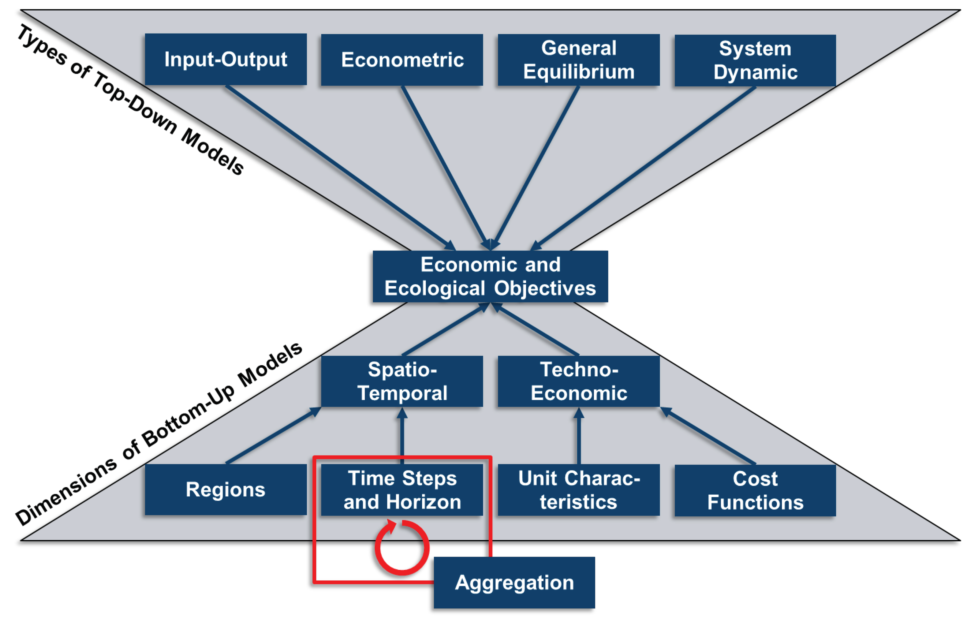
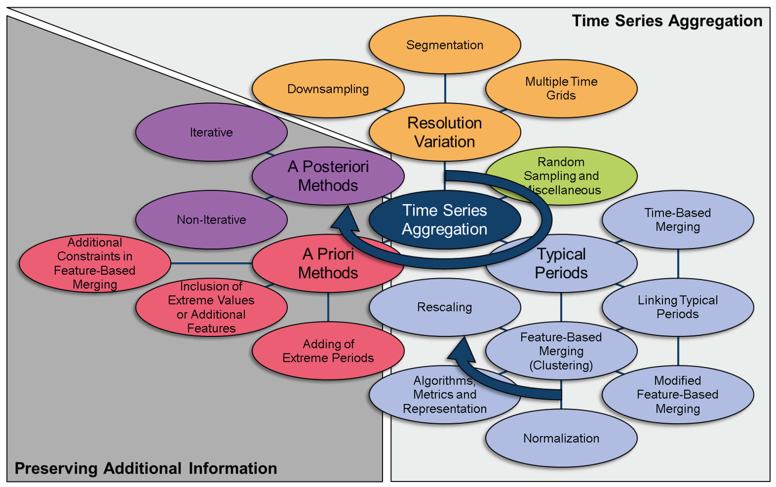
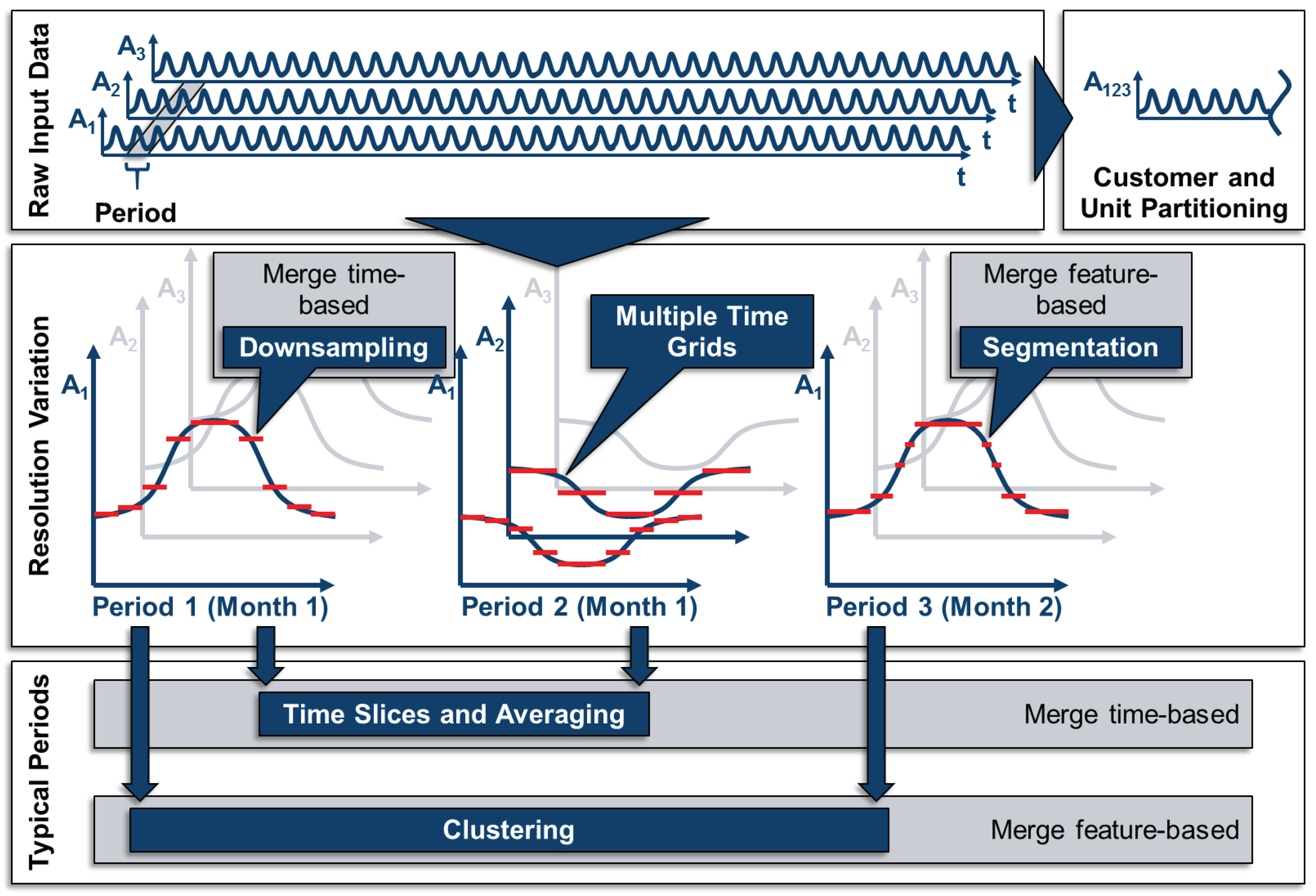
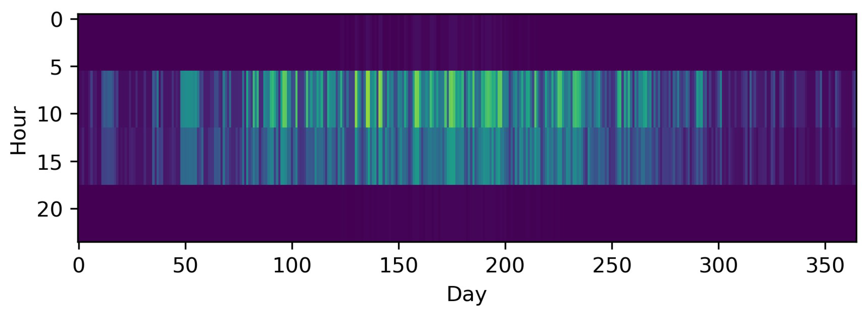
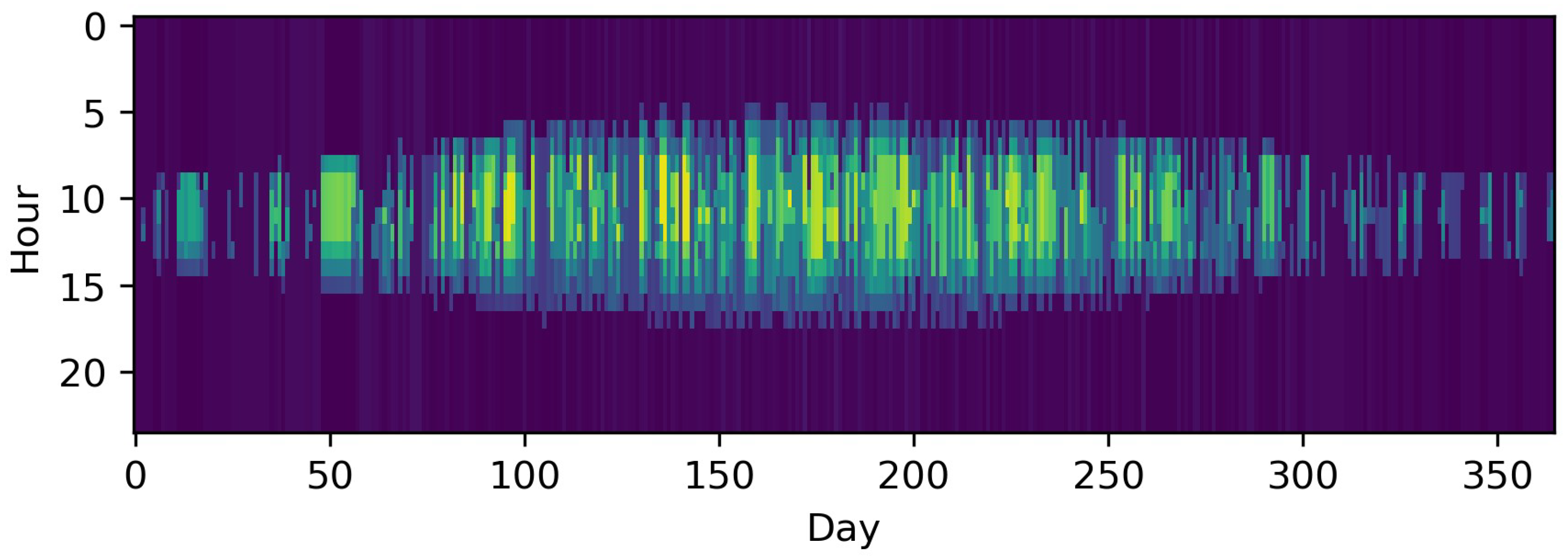
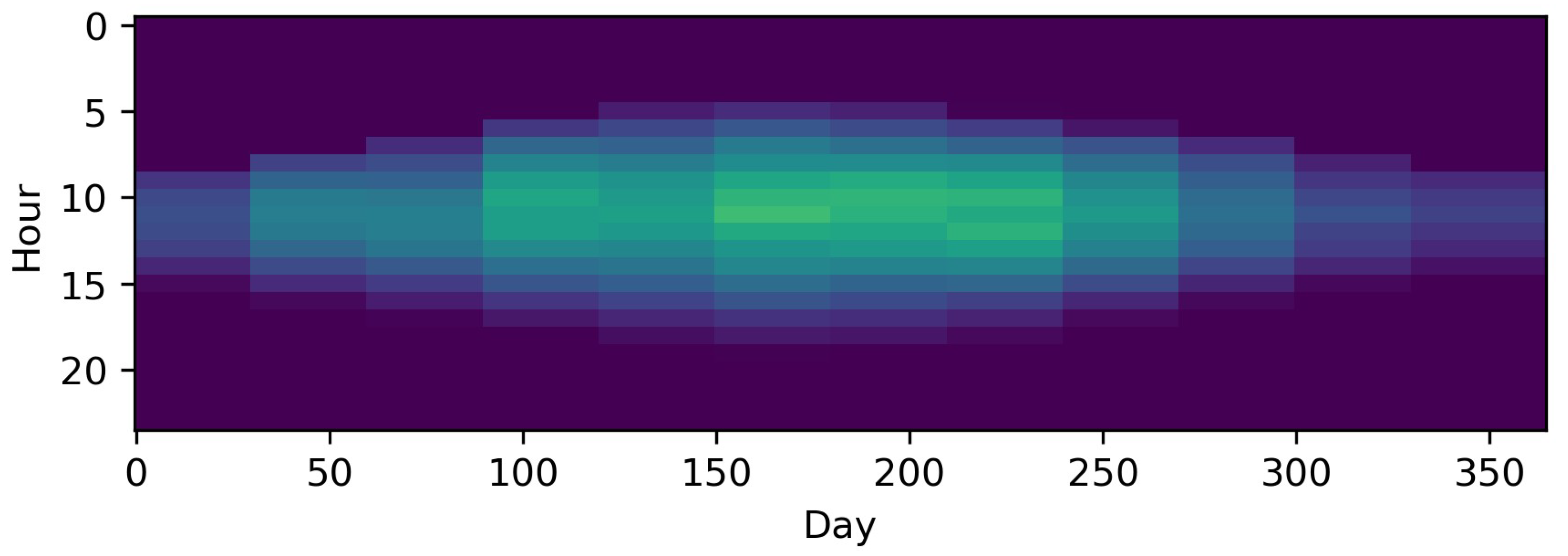
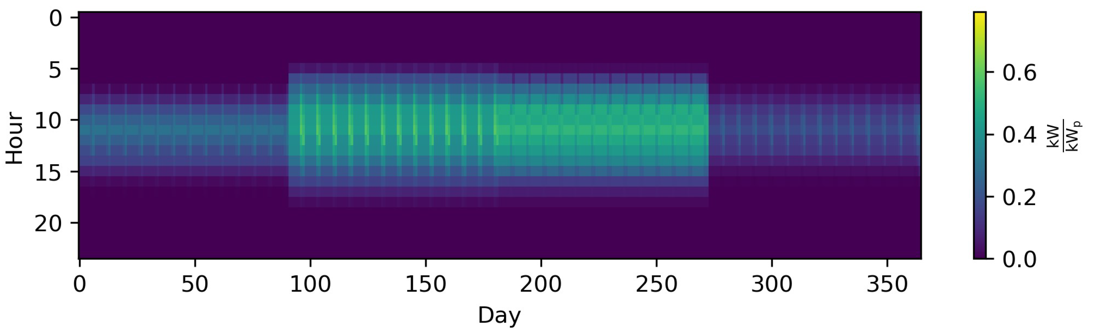
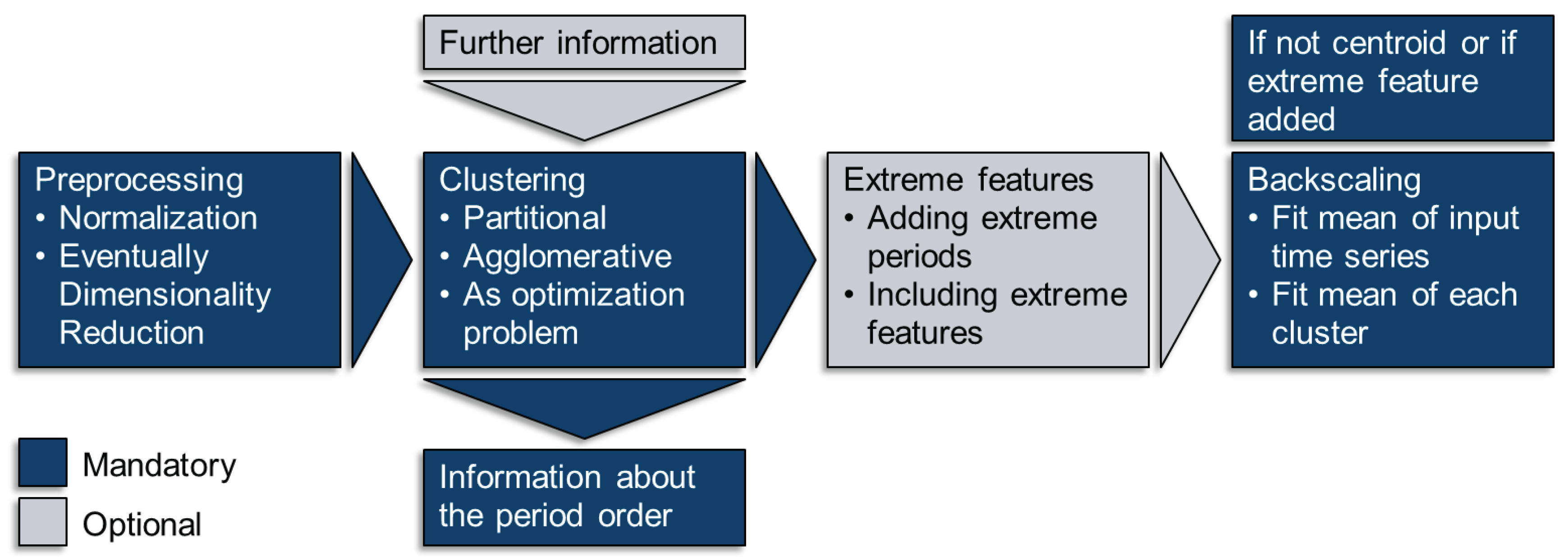
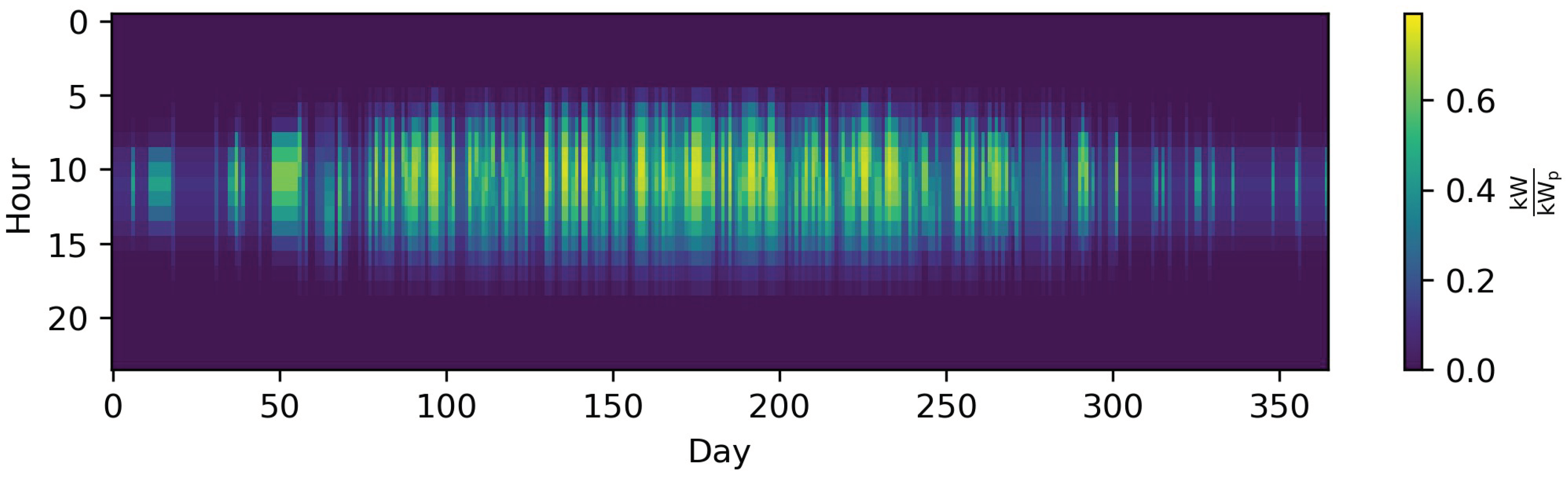
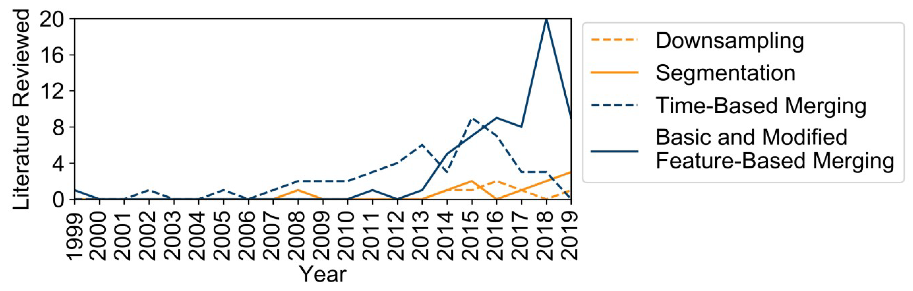
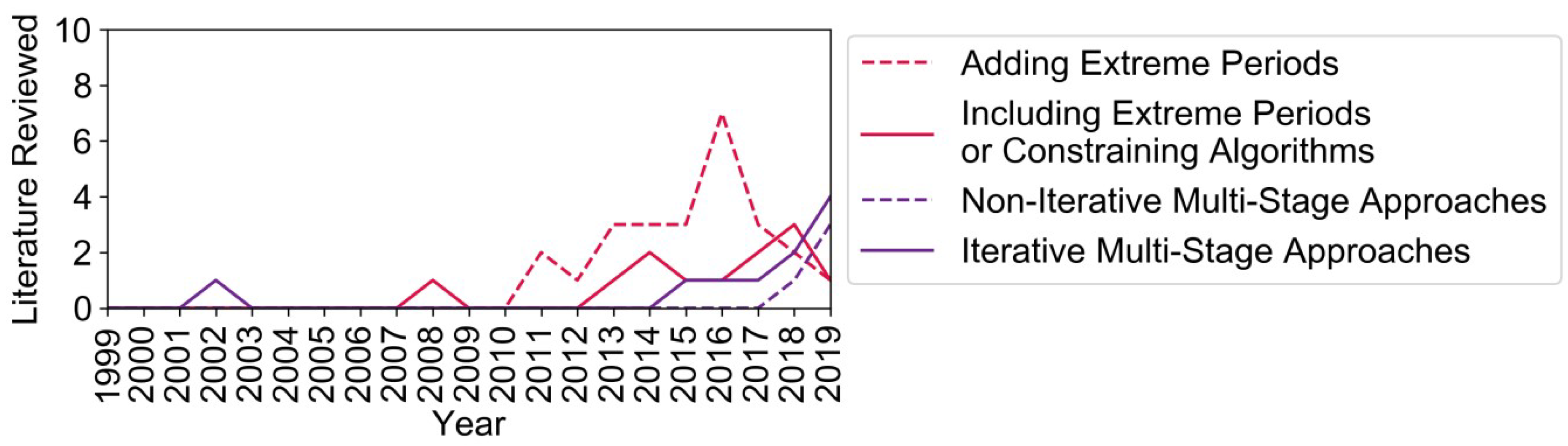
Table A1.
Table of Methods.
| Year | Author | ESM for Case Study, (Framework) | Normalization | Distance Metric | Clustering/Grouping | Representative | Extreme Periods | Linking Periods | Duration Curve |
|---|---|---|---|---|---|---|---|---|---|
| 1999 | Balachandra et al. [53] | None (just approach) | No | No | Multiple discriminant analysis | Mean | No | Yes | No |
| 2002 | Yokoyama et al. [66] | Building or district model, no storage technologies, but multiple commodities | No | No | Season-based (summer, mid-season, winter) with 4-, 2-, or 1- h resolution | (probably) Mean | No | No | No |
| 2007 | Lee et al. [183] | UC problem for 48 unit power system (not further specified) | No | No | No | No | No | Yes | No |
| 2007 | Swider et al. [122] | Single-node model for electricity production in Germany with wind and pumped hydro storage | No | No | Every two months, one weekday and one weekend day with 2-h resolution | (probably) Mean | No | No | No |
| 2008 | Marton et al. [98] | None (just approach) | No | Integral of absolute error (L1 norm) | Clustering by comparing each new day to clusters of preceding days | Mean | Yes, if outlier surpass a certain threshold of the IAE and the following day is close to the preceding cluster | Yes | No, although curve was called the duration curve |
| 2008 | Mavrotas et al. [54] | Building model for a hospital, no storage technologies, but multiple commodities | No | No | Monthly average | Mean | No | No | No |
| 2008 | Mavrotas et al. [54] | Building model for a hospital, no storage technologies, but multiple commodities | No/not mentioned | No/not mentioned | Seasonal rescaled average further segmented | Rescaled mean | Peak demand value of each cluster is kept for each attribute | No | No |
| 2009 | Alzate et al. [195] | Customer or unit partitioning/none (just approach) | Z-normalization | No (Hamming distance for out-of-sample extension) | Spectral clustering | None (just grouped) | No | No | No |
| 2009 | Casisi et al. [114] | District model, no storage technologies, but multiple commodities | No | No | Season-based (3 seasons for energy demand and 24 for sold energy to the grid) | (probably) Mean | No | No | No |
| 2009 | Lozano et al. [111] | Building model for a hospital, no storage technologies, but multiple commodities | No | No | Monthly average with distinction between weekday and weekend | (probably) Mean | No | No | No |
| 2010 | Lozano et al. [99] | District model, thermal storage units, multiple commodities | No | No | Monthly average | (probably) Mean | No | No | No |
| 2010 | Nicolosi et al. [104] | Single-node electricity dispatch model for Texas (ERCOT), no storage, technologies mentioned, (THEA) | No | No | Full resolution, 4 seasons, Wednesday, Saturday and Sunday with hourly resolution, 16 time slices | Means | No | No | No |
| 2011 | Domínguez-Muñoz et al. [55] | None (just approach) | Yes, but not mentioned which | Euclidean | k-medoids | Medoids | Peak heating and peak cooling day | No | No |
| 2011 | Haydt et al. [105] | Island electricity model for Flores (Azores), no explicitly modeled storage technologies (only via availability), (TIMES, LEAP, EnergyPlan) | No | No | LEAP: 9 time slices from the duration curve TIMES: 4 seasons, Wednesday, Saturday, and Sunday with hourly resolution EnergyPLAN: full hourly resolution | Means | No | Yes | LEAP: Yes TIMES: No |
| 2011 | Ortiga et al. [179] | Building model, thermal storage units, multiple commodities | No/not mentioned | No/not mentioned | Graphical method | Existing days | Peak heating and peak cooling day | No | Yes |
| 2011 | Pina et al. [124] | Island electricity model for São Miguel (Azores), no explicitly modeled storage technologies (only via availability), no storage technologies, (TIMES) | No | No | 4 seasons, weekday, Saturday and Sunday with hourly resolution | (probably) Mean | No | Yes | No |
| 2011 | Weber et al. [112] | Multi-node district model, daily heat and electricity storages, multiple commodities | No | No | 3 seasons further segmented into 6 irregular periods | (probably) Mean | No | No | No |
| 2012 | Buoro et al. [89] | Building model, thermal storage units, multiple commodities | No | No | Monthly average, typical weeks with 168 h | (probably) Mean | No | No | No |
| 2012 | Devogelaer et al. [125] | Multi-node model for Belgium, multiple storage technologies, multiple commodities, (JRC-EU-TIMES) | No | No | 26 2-week periods with three daily levels | (probably) Mean | Peak demand slice | Yes | No |
| 2012 | Mehleri et al. [129] | District model, no storage technologies, multiple commodities | No | No | 3 seasons further segmented into 6 irregular periods | (probably) Mean | No | No | No |
| 2012 | Van der Weijde et al. [180] | Multi-node electricity model for Great Britain, no explicitly modeled storage technologies (only as source/sink) | No | No | N hourly samples | Existing hours | No | No | No |
| 2012 | Welsch et al. [106] | Single-node electricity model for a town, battery storages, demand shifting, (OSeMOSYS) | No | No | In Proposal: 4 seasons, work days and weekends, 3 daily intervals. In example: Just one day in hourly resolution | (probably) Mean | No | Yes | No |
| 2013 | De Sisternes et al. [93] | Single-node electricity model, no storage technologies, but minimum up- and down-times | Min-max normalization for NLDC | Euclidean | Exhaustive search or heuristic | Existing weeks | Including peak week or peak day | No | Yes |
| 2013 | Kannan et al. [126] | Single-node electricity model for Switzerland and pumped hydro storage, (TIMES) | No | No | Season-based (four seasons and to diurnal time slices), or weekdays, Saturdays, Sundays in hourly resolution | Average | No | Yes | No |
| 2013 | Mehleri et al. [130] | District model, thermal storage units, multiple commodities | No | No | 3 seasons with hourly resolution | (probably) Mean | No | No | No |
| 2013 | Pina et al. [115] | Electricity model for Portugal, storage technologies considered, but modeling not explained, number of regions not mentioned, (TIMES and EnergyPLAN) | No | None | One weekday, one Saturday and one Sunday, 4 seasons | Not mentioned | No | No | No |
| 2013 | Simões et al. [127] | Multi-node model for Europe, multiple storage technologies, multiple commodities, (TIMES) | No | No | Season-based (four seasons, day, night and peak time slice) | Average | Average peak demand during each season | Yes | No |
| 2013 | Spiecker et al. [116] | Multi-node electricity model for Europe, hydro storage units, cogeneration units on regional scale | No/not mentioned | None | One weekday and one weekend day for every two months with 2 h resolution | Not mentioned | Yes, with stochastic approach | Yes | No |
| 2013 | Voll et al. [103] | District model, no storage technologies, multiple commodities | No | No | Monthly average | Mean | Two more time steps for summer and winter peak loads | No | No |
| 2014 | Adhau et al. [153] | Stochastic single-node electricity model, no storage technologies | No/not mentioned | Euclidean | k-means | Centroids | No | No | No |
| 2014 | Benítez et al. [196] | Customer or unit partitioning/none (just approach) | No/not mentioned (only one attribute) | Euclidean | Dynamic k-means | Centroids | No | Yes (yearly trajectory) | No |
| 2014 | Deane et al. [64] | UC of the Irish electricity system, pumped hydro storage, (PLEXOS) | No | No | Downsampling (5, 15, 30 and 60 min) | Average | No | Yes | No |
| 2014 | Fazlollahi et al. [138] | District heating model, no storage technologies | Min-max normalization | Euclidean | k-means | Centroids | Attribute peaks | No | No |
| 2014 | Fazlollahi et al. [69] | Two single-node district models with fixed capacities, no storage technologies, multiple commodities, UC (minimizing operating costs) | Min-max normalization | Euclidean | k-means and segmentation | Centroids | Attribute peaks | No | No |
| 2014 | Green et al. [154] | Electric dispatch model for UK, pumped hydro storage simulated, number of regions not mentioned | No (just two attributes of same scale clustered) | Euclidean | k-means | Centroids | Dominant ramp integration | No | No |
| 2014 | Poncelet et al. [36] | Island electricity model for Belgium, no storage technologies or transmissions, re-evaluation with UC model, (TIMES) | No | No | Season-based (four seasons, night, day and peak slice) | (probably) Mean | By choosing peak slice | No | No |
| 2014 | Stadler et al. [113] | Building model, multiple storage technologies, multiple commodities (DER-CAM) | No | No | (seven typical days or one typical weekday, one typical weekend day and one peak day) | (probably) Mean | Peak demand day in case of typical weekday and typical weekend day | No | No |
| 2014 | Wakui et al. [110] | Building model, thermal storage units, multiple commodities | No | No | Season-based | (probably) Mean | Peak summer day and peak winter day | No | No |
| 2014 | Wogrin et al. [85] | Single-node electricity model, no storage technologies | No (attributes of the same unit) | Euclidean | k-means, hourly, 6 system states | Centroids | No | No | No |
| 2014 | Xiao et al. [186] | Island electricity model for, no storage technologies | No | No | No | No | No | Yes | No |
| 2015 | Agapoff et al. [63] | Multi-node electricity model for GEP, no storage technologies | No/not mentioned | Euclidean | k-means, typical hours (snapshots) | Medoids | Included as clustered features (min, max, std., local difference and avg.) | No | No |
| 2015 | Brodrick et al. [155] | Single-node model of a coal-plant with alternative natural gas and solar thermal heat sources and carbon capture and storage, CO2 solvent storage unit, multiple commodities | Normalization by dividing by the average | Euclidean | k-means | Centroids | No | No | No |
| 2015 | Bungener et al. [70] | UC of a chemical cluster, multiple commodities | Normalized by average values and multiplied by weight | None, but variance indicator and zero flowrate indicator | Evolutionary mechanisms (segmentation) | Means | No | Yes (adjacent time steps are merged) | No |
| 2015 | Deml et al. [71] | Single-node electric dispatch model, pumped hydro storage | No | No | Progressive downsampling | Means | No | Yes | No |
| 2015 | Fitiwi et al. [142] | IEEE 24-bus Reliability Test System [197], multi-node electricity model, no storage technologies | Normalized by maximum line length and base load | Euclidean | k-means, typical hours (snapshots) | Medoids closest to the clusters’ centroids | No | No | No |
| 2015 | Harb et al. [101] | Building model and district model, thermal storage units, multiple commodities | No | No | Monthly average, also 15 min. and hourly resolution | Mean | No | No | No |
| 2015 | Harb et al. [90] | District model, thermal and battery storage units, multiple commodities | No | No | Cluster by sums of weeks (sensitivity analysis also for different day numbers), typical weeks | Means | No | No | No |
| 2015 | Marquant et al. [149] | District heating model, no storage technologies, multiple commodities | No/not mentioned | Euclidean | k-medoids | Medoids | Peak electricity and peak heating days | No | Yes |
| 2015 | Merkel et al. [91] | District model, thermal storage units, multiple commodities | No | No | Season based (three weeks from spring/autumn, summer and winter), 15 min. resolution | (probably) Existing weeks | No | No | No |
| 2015 | Munoz et al. [181] | IEEE Reliability Test System [188], multi-node electricity model, no storage technologies | No/not mentioned | Euclidean | Daily moment-matching, k-means for hours, typical hours (snapshots) | Centroids | Top 10 peak load hours included | No | No |
| 2015 | Poncelet et al. [177] | None (just approach) | No/not mentioned | L1-Norm | Using so-called “bins” | Existing days | No | No | Yes |
| 2015 | Samsatli et al. [16] | Multi-node island model, multiple hydrogen storage technologies, multiple commodities | No | No | Season-based (four seasons, weekdays and weekend days) | (probably) Mean | No | Yes | No |
| 2015 | Schiefelbein et al. [163] | District model, thermal storage units, multiple commodities | No/not mentioned | Euclidean | k-medoids | Medoids | No | No | |
| 2015 | Wakui et al. [109] | Building model, thermal and battery storage units, multiple commodities | No | No | Season based | (probably) Mean | Peak summer day and peak winter day | No | No |
| 2015 | Wouters et al. [117] | District model, heat, cold and battery storage technologies, multiple commodities | No | No | Season-based (spring/autumn, summer and winter) | (probably) Mean | Sensitivity analysis by adding variability to PV input data | No | No |
| 2015 | Yang et al. [118] | District model, heat and cold storage technologies, multiple commodities | No | No | Season-based (spring/autumn, summer and winter), 2 h resolution | (probably) Mean | No | No | No |
| 2015 | Yokoyama et al. [67] | Building model for a hotel, no storage technologies, but multiple commodities | No | No | Season-based (summer, mid-season, winter) with 8, 4, or 2 h resolution and for commercial solver 1 h | (probably) Mean | No | No | No |
| 2016 | Ameri et al. [119] | District model no storage technologies, multiple commodities | No | No | Season-based (summer and winter) | (probably) Mean | No | No | No |
| 2016 | Beck et al. [65] | Electric building model, battery storage | No | No | Single day downsampled (10, 30, 60, 300, 900, 3600 s), analyzed single days | Mean | No | Yes | No |
| 2016 | Bracco et al. [120] | District model, thermal and battery storage technologies, multiple commodities, (DESOD) | No/not mentioned | No | Season-based (summer, winter, mid-season) | (probably) Mean | No | No, initial conditions at each day, e.g., | No |
| 2016 | De Sisternes et al. [92] | Single-node electricity model, battery storage and minimum up- and down-times | Min-max normalization for NLDC | Euclidean | Exhaustive search or heuristic (refers to [93], but with additional cycled power error), typical weeks | Existing weeks | Including peak week or peak day | No | Yes |
| 2016 | Frew et al. [182] | Multi-node electric model of the US, pumped hydro, thermal and battery storage technologies, (POWER) | Yes, but not mentioned is which, but averaged across all potential developable sites | None | Random days | Existing days, weights calculated with least squares method | Extreme days containing the peak value for each of the eight attributes | No (net storage values of each day must be zero or SOC at start of each day equals that at the end) | Yes |
| 2016 | Haikarainen et al. [198] | Customer or unit partitioning/district model, thermal storage units, multiple commodities | No | Euclidean | k-means | Means | No | No | No |
| 2016 | Kools et al. [102] | District electricity model, battery storage units, heat demand driven CHP units considered | No | No | Averaging of eight consecutive weeks in each season to one typical day | Mean | Normal distributions added for 1 min, 15 min and 1 h resolution (stochastic impact) | Control policy for the storage (not across days) | No |
| 2016 | Lin et al. [156] | Multiple building models, thermal and battery storage units, multiple commodities | No/not mentioned (attributes of the same unit) | Euclidean | k-means | Existing day which is closest to the centroid | No | No (periodic SOC) | No |
| 2016 | Lythcke-Jørgensen et al. [88] | CHP-plant model, no storage technologies, multiple commodities | Heat demand normed by maximum value | No/not mentioned | So-called “CHOP” aggregation (graphical method) for five years of hourly data | Means | No | No | No |
| 2016 | Merrick et al. [40] | Single-node electricity model, no storage technologies | No | None | Monthly median and peak electricity demand day with 4 h resolution and only one averaged period | Medoids | Peak electricity demand days | No | No |
| 2016 | Nahmmacher et al. [143] | Multi-node electricity model LIMES-EU [199] with intraday storage technologies, (LIMES-EU) | Demand: region-specific divided by maximum value VRE: divided by maximum value across all regions | Euclidean | hierarchical | Medoids | No | No | No |
| 2016 | Oluleye et al. [123] | Single-node district model, thermal storage units, multiple commodities | None | None | One weekday and one weekend day for winter, summer and transition with 7 (6) time bands (slices) | Not mentioned | No | No | No |
| 2016 | Patteeuw et al. [94] | Building heating model of nine buildings, thermal storage units, multiple commodities | No/not mentioned, Demand: region-specific divided by maximum value | L1-Norm | Using so-called “bins”, heuristic, hierarchical clustering according to Nahmmacher et al. [143] for the years of 2013–2016 | Existing weeks (6) | Coldest week and week with highest e-demand (same week) | No | Yes |
| 2016 | Ploussard et al. [87] | IEEE 24-bus Reliability Test System [197], multi-node electricity model, no storage technologies | No/not mentioned | Euclidean | k-means, typical hours (snapshots) | Existing snapshot closest to the centroids | No | No | No |
| 2016 | Poncelet et al. [128] | Island electricity model for Belgium, no storage technologies or transmissions, re-evaluation with UC model, (TIMES) | No | None | For each of the four seasons one night, day and peak electricity time slice | Mean | Peak electricity time slice | No | No |
| 2016 | Poncelet et al. [144] | Single-node electricity model based on [200], no storage technologies, (LUSYM) | No/not mentioned, Demand: region-specific divided by maximum value | L1-Norm, Euclidean | Using so-called “bins”, heuristic, hierarchical clustering according to Nahmmacher et al. [143] | Existing days, medoids | No, for heuristics days with highest and lowest value for e-demand and highest and lowest average for wind and PV | No | Yes |
| 2016 | Samsatli et al. [17] | Multi-node hydrogen-electricity model for Great Britain, multiple hydrogen storage units, multiple commodities | No | No | Season-based (four seasons, work days and weekend days) | (Probably) Mean | No | Yes | No |
| 2016 | Schütz et al. [139] | Building model, thermal and battery storage units, multiple commodities | Min-max normalization | Euclidean | k-means k-medians k-medoids k-centers | Centroids Medians Medoids Centers | No | No | No |
| 2016 | Stenzel et al. [38] | UC of building electricity model with battery storage | No | None | downsampling | Means | No | Yes | No |
| 2016 | Wakui et al. [108] | Building model, thermal and battery storage units, multiple commodities | No | No | Season based | (probably) Mean | Peak summer day and peak winter day | No | No |
| 2016 | Wogrin et al. [83] | Single-node electricity model, pumped hydro and battery storage | No/not mentioned | Euclidean | k-means (98 system states (typical hours)) | Centroids | No, but the first and last hour of the time horizon were manually added | Yes | No |
| 2017 | Bahl et al. [157] | District model from Voll et al. [103], no storage technologies, multiple commodities | No/not mentioned (attributes of same scale clustered) | (probably) Euclidean | k-means, typical hours (snapshots) | Centroids | Feasibility time steps (peak values) and operation optimization for full time series | No | No |
| 2017 | Brodrick et al. [146] | UC of an integrated solar combined cycle, no storage technologies, multiple commodities | Z-normalization | Euclidean | k-means | Centroids | No | No | No |
| 2017 | Härtel et al. [86] | Multi-node transmission expansion planning model, no storage technologies | Either normed by highest value per market or highest value across all markets | Euclidean | k-means, k-medoids, hierarchical, systematic sampling, moment-matching, typical hours (snapshots) | Centroids, medoids, sample points | Heurisitc defining new cluster centers if 95% of a cluster’s data points are below or above a 6 h moving average, with the lowest or highest chosen as the new cluster center | No | No |
| 2017 | Heuberger et al. [158] | Single-node electricity model with carbon capture and storage and grid-level storage | Yes, but not mentioned which | Euclidean | k-means | Means | Day with annual electricity peak demand | No | No |
| 2017 | Marquant et al. [150] | District heating model, thermal and battery storage units, multiple commodities | No/not mentioned | Euclidean | k-medoids | Medoids | Peak electricity and peak heating days | No | Yes |
| 2017 | Moradi et al. [121] | Single-node model of an energy hub, thermal and battery storage, multiple commodities | No | No | Season-based (one work day and one weekend day per spring, summer, autumn and winter) | (probably) Mean | No | No | No |
| 2017 | Pfenninger et al. [37] | Multi-node electricity model for Great Britain, pumped hydro and battery storage units | Normalized by the maximum value across all time steps and model zones | Euclidean | k-means, hierarchical, downsampling, heuristics | Centroids, medoids | Min/max solar and wind days, wind and PV weeks and wind-demand weeks | No | No |
| 2017 | Renaldi et al. [61] | Single-node district heating system, long- and short-term thermal storage units, multiple commodities | No | None | Multiple time grids for different storage technologies | Downsampled 3 h steps for long-term storage | No | Yes | No |
| 2017 | Timmerman et al. [107] | Two business park models (one based on the model of Voll et al. [103]), thermal and electrical storage units, multiple commodities, (Syn-E-Sys) | No | No | Season and weekday-based (4 × 2 × 4 6 h intervals) | (probably) Mean | No | Yes | No |
| 2017 | Schütz et al. [100] | Building model, thermal and battery storage units, multiple commodities | No | No | Monthly average (one typical day per month and weighted) | (probably) Mean | No | No | No |
| 2017 | Sun et al. [136] | Customer or unit partitioning/none (just approach) | Time steps wise (in period) average s divided by maximum value of each customer | Likelihood-function | Vine-copula mixture model | None | No | No | No |
| 2017 | Teichgräber et al. [147] | Oxyfuel natural gas plant, liquid oxygen storage, multiple commodities | Z-Normalization | Euclidean | k-means | Centroids | No | No | No |
| 2017 | vom Stein et al. [79] | Multi-node electricity dispatch model for Europe, pumped hydro storage | No | L1-Norm | Clustering of consecutive time steps with objective to minimize gradients within clusters | Mean | No | Yes (clustering of consecutive time steps) | No |
| 2017 | Yang et al. [201] | Customer or unit partitioning/none (just approach) | Z-normalization | Shape-based distance | k-shape | None | No | No | No |
| 2017 | Zhu et al. [164] (refers to [55]) | Building model for an airport in China optimizing economics or CO2 emissions, no storage technologies, but start-up and shut-down costs | Yes, but not mentioned which | Euclidean | k-medoids (only three season-specific typical days) | Medoids | No | No | No |
| 2018 | Almaimouni et al. [137] | Single-node GEP for electricity, validated with rolling horizon UC, no storage technologies | Normalize by with m as number of days, principal components | Euclidean | k-means | Centroids | No | No | Only as error estimator |
| 2018 | Bahl et al. [192] | District model from Voll et al. [103] and a single-node pump system, no storage technologies, multiple commodities | No/not mentioned (attributes of same scale clustered) | Euclidean | k-means, typical hours (snapshots) | Undersestimators from minimum values of each cluster | Feasibility time steps (peak values) and operation optimization for full time series | No | No |
| 2018 | Bahl et al. [74] | District model from Voll et al. [103] with additional heat and cold storage units, multiple commodities | Yes, but not mentioned which | Euclidean | k-medoids (daily clustering and segmentation) | Medoids further segmented | Feasibility time steps (peak values) and operation optimization for full time series | No | No |
| 2018 | Brodrick et al. [97] refers to [146] | UC of an integrated solar combined cycle, no storage technologies, multiple commodities | Z-normalization | Euclidean | k-means (6 representative days) further reduced to three extreme hours | Centroids | Three extreme hours | No | No |
| 2018 | Gabrielli et al. [15] | Single-node district model, thermal, battery and hydrogen storage, multiple commodities | No/not mentioned | Not mentioned (probably Euclidean/default for Matlab k-means) | k-means | Centroids | Maximum and minimum values of the demand profiles | Yes | No |
| 2018 | Kotzur et al. [57] | Three single-node models (CHP system, residential building, island system), thermal, battery and hydrogen storage, multiple commodities | Min-max normalization | Euclidean | k-means, averaging, k-medoids, hierarchical, typical days and typical weeks | Centroids medoids | Peak periods heat and electricity demand, minimum PV feed-in | No | No |
| 2018 | Kotzur et al. [14] | Three single-node models (CHP system, residential building, island system), thermal, battery and hydrogen storage, multiple commodities | Min-max normalization | Euclidean | Exact k-medoids | Medoids | No | Yes | No |
| 2018 | Lara et al. [24] | Multi-node electricity model for Texas, multiple storage units (e.g., lithium-ion, lead-acid, and flow batteries) | Mentioned, but not which one | Euclidean | k-means for the years of 2004–2010 | Centroids | No | No, 50% SOC heuristic | No |
| 2018 | Liu et al. [148] | Multi-node electricity model for Texas (greenfield GEP), storage units and ramping constraints considered | Z-Normalization | DTW distance, Euclidean as benchmark | (k-means initially), hierarchical, k-means as benchmark | Medoids, centroids for k-means-benchmark | No | No | No |
| 2018 | Mallapragada et al. [39] (2004–2010) | Electricity GEP model for Texas, no storage or transmission units, ramping in production cost simulation considered | Min-max normalization between 0 and 2 | Euclidean and L1-Norm (as benchmark) | 4 seasons and 4 daily segments vs. k-means | Medoids | No | No, refers to [24], 50% heuristic | No |
| 2018 | Neniškis et al. [51] | Electricity and district heat model of Lithuania, pumped hydro storage, multiple commodities, (MESSAGE) | No | None | Workday and weekend day either for four seasons or for twelve months | Mean | No (but synthesized wind time series) | No | No |
| 2018 | Pineda et al. [72] | Multi-node electricity model of Europe, intraday, interday storage and ramping constraints considered | Mentioned, but not which one | Euclidean | Hierarchical | Medoids | No | Yes, by clustering adjacent periods | No |
| 2018 | Schütz et al. [58] | Building model, thermal and battery storage units, multiple commodities | Min-max normalization | Euclidean | k-means k-medians k-medoids k-centers | Centroids medians medoids centers | No | No | No |
| 2018 | Stadler et al. [165] | Building model, thermal and battery storage units, multiple commodities | No/not mentioned | (probably) Euclidean | k-medoids | Medoids | No | No | No |
| 2018 | Teichgräber et al. [159] | Two minimal UC problems: An electricity storage model and a gas turbine dispatch model | Element-wise Z-Normalization | Euclidean, Dynamic Time Warping, Shape-based Distance | k-means k-medoids Barycenter Averaging k-shape hierarchical | Centroid, medoids | No | No | No |
| 2018 | Tejada-Arango et al. [19] | UC of the Spanish electricity system, battery and pumped hydro storage | Yes, but not mentioned what kind of normalization | (probably) Euclidean | k-medoids for RP, k-means for SS | Medoids, centroids | No | Yes | No |
| 2018 | Tejada-Arango et al. [84] | UC of the IEEE 14 bus electricity model, battery and pumped hydro storage | No/not mentioned (attributes of same scale clustered) | Euclidean | k-means (for typical hours) | Centroids | No | No | No |
| 2018 | Tupper et al. [167] | UC of the IEEE 30 bus electricity model with wind generation, no storage technologies | No/not mentioned | Euclidean, band distance | k-medoids | Medoids | No | No | No |
| 2018 | Van der Heijde et al. [95] | Single-node district heating model, thermal storage | No/not mentioned | L1-Norm | Using so-called “bins” and four seasons | Existing weeks | No, but each season needs to contain at least one typical week | Yes | Yes |
| 2018 | Voulis et al. [145] | Customer or unit partitioning/none (just approach) | Normalization by maximum e-demand | Euclidean | k-means (spatio-temporal differentiation between workdays, weekends, neighborhoods, districts and municipalities) | Centroids | No | No | No |
| 2018 | Welder et al. [18] | Multi-node model for power-to- hydrogen in Germany, hydrogen storage technologies, multiple commodities | Min-max normalization | Euclidean | hierarchical | Medoids | No | Yes | Yes |
| 2019 | Baumgärtner et al. [78] | District model from Voll et al. [103] with additional heat and cold storage units and a single-node pump system, multiple commodities | No/not mentioned | Euclidean | k-medoids | Segmented under- and overestimators | Feasibility time steps (peak values) and operation optimization for full time series | No | No |
| 2019 | Baumgärtner et al. [77] | Single-node model for industrial site based on Baumgärtner et al. [202] with heat, cold and battery storage, Multi-node model for Germany with battery and hydrogen storage, multiple commodities | No/not mentioned | Euclidean | k-means | Centroids, segmented under- and overestimators | Feasibility time steps (peak values) and operation optimization for full time series | Yes | No |
| 2019 | Gabrielli et al. [160] | Single-node district model, thermal, battery and hydrogen storage, multiple commodities | No/not mentioned | Not mentioned (probably Euclidean/default for Matlab k-means) | k-means | Centroids | Maximum and minimum values of the demand profiles | Yes | No |
| 2019 | Hilbers et al. [166] | Single-node electricity model of Great Britain, no storage technologies | Yes, but not mentioned which | Euclidean | Samples (hourly). As benchmark: k-medoids (days) | Existing hours. As benchmark: medoids (days) | Yes with the method of subsampling and keeping the most expensive days | No | No |
| 2019 | Kannengießer et al. [140] | Multi-node district model and single-node island model, thermal, battery and hydrogen storage, multiple commodities | Min-max normalization | Euclidean | hierarchical | Medoids | No, but operation optimization for full time series | No | Yes |
| 2019 | Motlagh et al. [203] | Customer or unit partitioning/none (just approach) | No/not mentioned | Adjacency metric, in mapping parameter space: Euclidean d | Feature-based clustering or dynamic load-clustering | None | No | No | No |
| 2019 | Pavičević et al. [204] | Customer or unit partitioning/multi-node electricity model of the western Balkan, pumped hydro storage and CHP with thermal storage, (Dispa-SET) | No | None | By technology and location | Mean | No | No | No |
| 2019 | Pöstges et al. [187] | Single-node electricity model, no storage technologies, analytically solved as peak-load-pricing model | Yes, cap-specific costs | None | Segments in the duration curve implying use of different technologies (hours) | Sorted existing hours | Yes, by determining the capacity of each component from the merit order | No | Yes |
| 2019 | Savvidis et al. [80] | UC of dispatch electricity model for Germany, pumped hydro storage, (E2M2) | No | No | No | No | Certain time series qualities define intervals in which can be downsampled | Yes, by clustering adjacent periods | No |
| 2019 | Sun et al. [135] | Multi-node electricity model of Great Britain with intraday storage | Min-max normalization, dimensionality reduction applied | Euclidean | hierarchical | Medoids | No | No | No |
| 2019 | Teichgräber et al. [41] | Two minimal UC problems: An electricity storage model and a gas turbine dispatch model | Element-wise Z-Normalization | Euclidean, Dynamic Time Warping, Shape-based Distance | k-means k-medoids Barycenter Averaging k-shape hierarchical | Centroid, medoids | No | No | No |
| 2019 | Van der Heijde et al. [20] | Multi-node district heating model, thermal storage | No/not mentioned | L1-Norm | Using so-called “bins” | Existing days | No, but rearranging the typical days to the original sequence using a MIP | Yes | Yes |
| 2019 | Yokoyama et al. [68] | Building model for two hotels and four office buildings, no storage technologies, but multiple commodities | No | None | downsampling | Means | No | No | No |
| 2019 | Zatti et al. [141] | District model of Parma university campus and building model, thermal and battery storage, multiple commodities | Min-max normalization | Euclidean | (k-means, k-medoids) k-MILP (modification of k-medoids) | (Centroids), medoids | Automatically integrating atypical days | No | No |
| 2019 | Zhang et al. [161] | Single-node electricity model consisting of hydro, PV and wind power plants with reservoir storage | No/not mentioned | Euclidean | k-means | Means | No, but used Vine-Copula, ARMA-model and latin hypercube sampling to generate scenarios | No | No |
Appendix B
Customer and Unit Partitioning
It is noteworthy that aggregations based on time series do not necessarily mean the aggregation of the temporal dimension. Instead, similar time series can also be clustered in order to generate a smaller number of possible technologies or regions with similar demand behavior or similar technologies. This is referred to as customer [136] and unit [204] partitioning. Given the fact that, in some cases, new methods were first introduced in this field of TSA, a short overview of methods used in this field could imply possible approaches for the TSA methods presented above.
One of these examples was published by Alzate et al. [195], who used spectral clustering with an out-of-sample extension to cluster customer profiles for electricity demand. For this, 123 time series were used for training and 122 for validation. The approach significantly outperformed the selection found by k-means clustering. Benítez et al. [196] implemented a modified version of k-means for customer partitioning that was not only capable of clustering groups of customers with their daily profiles, but also with respect to their yearly profiles. This means that each cluster center of a (daily) period followed a trajectory throughout the year resulting in representative yearly profiles. Sun et al. [136] used a C-vine copula-based mixture model to cluster residential electricity demands by maximizing a log-likelihood function, which slightly outperformed k-means clustering but was computationally significantly more demanding. Yang et al. [201] used k-shape clustering for forming typical residential daily profiles before applying it to TSA purposes. This highlights the importance of cross-linking different research fields within energy system analysis. Recently, Motlagh et al. [203] applied two different clustering algorithms on electricity demands for customer partitioning. The first one included a preliminary principal component analysis to decrease the complexity, followed by clustering using the adjacency metric, while the second one was model-based and transferring the profiles into the phase space. Then, a mapping strategy based on neural regression was used and the Euclidean distance between the map parameters was calculated, which outperformed the first, feature-based approach.
With respect to unit partitioning, Pavičević et al. [204] introduced three levels of potential clustering scopes. The first was based on similar characteristics if the components were small, at the same location, with the same commodities and comparable temporal characteristics, while the second focused on the same location and the same commodities and the third only on the same commodities, such as averaged heat and electricity demands of industrial sites and residential buildings. Haikarainen et al. [198] used k-means clustering for grouping different nodes in an energy network that were then represented as a single component with averaged costs and the traits of all of the included technologies (supply, demand, storage). Based on decisions made for a coarse clustering, the number of clusters was stepwise increased and, in a final run, all binary decision variables were retained and a linear problem was solved for the fully resolved energy grid. This means that the clustering was not based on temporal features, but on spatial ones. This means that the units were merged based on their distance to each other, not their traits.
This highlights that temporal, spatial, and technological information can theoretically be aggregated based on their own or based on each other. Thus, TSA is traditionally seen as the aggregation of time series derived from temporal information.
Appendix C
Calculation Example for Time Series Normalization
In the following, a hypothetical time series is normalized as per Equations (1)–(3). The time series is given as six-dimensional row vectors including only positive values, representing 4 h intervals of electricity demand in kW for January 1st:
Min-Max-Normalization:
Max-Normalization:
Z-Normalization:
This means:
References
- Robinius, M.; Otto, A.; Heuser, P.; Welder, L.; Syranidis, K.; Ryberg, D.S.; Grube, T.; Markewitz, P.; Peters, R.; Stolten, D. Linking the Power and Transport Sectors—Part 1: The Principle of Sector Coupling. Energies 2017, 10, 956. [Google Scholar] [CrossRef] [Green Version]
- Barnett, H.J. Energy Uses and Supplies 1950, 1947, 1965, Bureau of Mines: Washington, DC, USA, 1950.
- Boiteux, M. La Tarification des Demandes en Pointe. Rev. Gen. De L’electricite 1949, 58, 157–179. [Google Scholar]
- Boiteux, M. Peak-Load Pricing. J. Bus. 1960, 33, 157–179. [Google Scholar] [CrossRef]
- Steiner, P.O. Peak loads and efficient pricing. Q. J. Econ. 1957, 71, 585–610. [Google Scholar] [CrossRef]
- Sherali, H.D.; Soyster, A.L.; Murphy, F.H.; Sen, S. Linear programming based analysis of marginal cost pricing in electric utility capacity expansion. Eur. J. Oper. Res. 1982, 11, 349–360. [Google Scholar] [CrossRef]
- Helm, D. Energy policy: Security of supply, sustainability and competition. Energy Policy 2002, 30, 173–184. [Google Scholar] [CrossRef]
- Hoffman, K.C.; Wood, D.O. Energy System Modeling and Forecasting. Annu. Rev. Energy 1976, 1, 423–453. [Google Scholar] [CrossRef]
- Lopion, P.; Markewitz, P.; Robinius, M.; Stolten, D. A review of current challenges and trends in energy systems modeling. Renew. Sustain. Energy Rev. 2018, 96, 156–166. [Google Scholar] [CrossRef]
- Caramanis, M.C.; Tabors, R.D.; Nochur, K.S.; Schweppe, F.C. The Introduction of Non-Dispatchable Technologies as Decision Variables in Long-Term Generation Expansion Models. Ieee Power Eng. Rev. 1982, PER-2, 40–41. [Google Scholar] [CrossRef]
- Bhattacharyya, S.C.; Timilsina, G.R. A review of energy system models. Int. J. Energy Sect. Manag. 2010, 4, 494–518. [Google Scholar] [CrossRef]
- Pfenninger, S.; Hawkes, A.; Keirstead, J. Energy systems modeling for twenty-first century energy challenges. Renew. Sustain. Energy Rev. 2014, 33, 74–86. [Google Scholar] [CrossRef]
- Ringkjøb, H.-K.; Haugan, P.M.; Solbrekke, I.M. A review of modelling tools for energy and electricity systems with large shares of variable renewables. Renew. Sustain. Energy Rev. 2018, 96, 440–459. [Google Scholar] [CrossRef]
- Kotzur, L.; Markewitz, P.; Robinius, M.; Stolten, D. Time series aggregation for energy system design: Modeling seasonal storage. Appl. Energy 2018, 213, 123–135. [Google Scholar] [CrossRef] [Green Version]
- Gabrielli, P.; Gazzani, M.; Martelli, E.; Mazzotti, M. Optimal design of multi-energy systems with seasonal storage. Appl. Energy 2018, 219, 408–424. [Google Scholar] [CrossRef]
- Samsatli, S.; Samsatli, N.J. A general spatio-temporal model of energy systems with a detailed account of transport and storage. Comput. Chem. Eng. 2015, 80, 155–176. [Google Scholar] [CrossRef]
- Samsatli, S.; Staffell, I.; Samsatli, N.J. Optimal design and operation of integrated wind-hydrogen-electricity networks for decarbonising the domestic transport sector in Great Britain. Int. J. Hydrog. Energy 2016, 41, 447–475. [Google Scholar] [CrossRef]
- Welder, L.; Ryberg, D.; Kotzur, L.; Grube, T.; Robinius, M.; Stolten, D. Spatio-Temporal Optimization of a Future Energy System for Power-to-Hydrogen Applications in Germany. Energy 2018, 158, 1130–1149. [Google Scholar] [CrossRef]
- Tejada-Arango, D.A.; Domeshek, M.; Wogrin, S.; Centeno, E. Enhanced Representative Days and System States Modeling for Energy Storage Investment Analysis. IEEE Trans. Power Syst. 2018, 33, 6534–6544. [Google Scholar] [CrossRef] [Green Version]
- van der Heijde, B.; Vandermeulen, A.; Salenbien, R.; Helsen, L. Representative days selection for district energy system optimisation: A solar district heating system with seasonal storage. Appl. Energy 2019, 248, 79–94. [Google Scholar] [CrossRef]
- Ören, T.I. Computer-Aided Systems technology: Its role in advanced computerization. In Computer Aided Systems Theory; Pichler, F., Moreno Díaz, R., Eds.; Springer Berlin Heidelberg: Berlin/Heidelberg, Germany, 1994; pp. 11–20. [Google Scholar]
- Sass, S.; Mitsos, A. Optimal Operation of Dynamic (Energy) Systems: When are Quasi-Steady Models Adequate? Comput. Chem. Eng. 2019. [Google Scholar] [CrossRef]
- Morales-España, G.; Tejada-Arango, D. Modelling the Hidden Flexibility of Clustered Unit Commitment. IEEE Trans. Power Syst. 2018.
- Lara, C.L.; Mallapragada, D.S.; Papageorgiou, D.J.; Venkatesh, A.; Grossmann, I.E. Deterministic electric power infrastructure planning: Mixed-integer programming model and nested decomposition algorithm. Eur. J. Oper. Res. 2018, 271, 1037–1054. [Google Scholar] [CrossRef]
- Lopion, P.; Markewitz, P.; Stolten, D.; Robinius, M. Cost Uncertainties in Energy System Optimisation Models: A Quadratic Programming Approach for Avoiding Penny Switching Effects. Energies 2019, 12, 4006. [Google Scholar] [CrossRef] [Green Version]
- Klinge Jacobsen, H. Integrating the bottom-up and top-down approach to energy–economy modelling: The case of Denmark. Energy Econ. 1998, 20, 443–461. [Google Scholar] [CrossRef] [Green Version]
- Subramanian, A.; Gundersen, T.; Adams, T. Modeling and simulation of energy systems: A review. Processes 2018, 6, 238. [Google Scholar] [CrossRef] [Green Version]
- Böhringer, C.; Rutherford, T.F. Integrating bottom-up into top-down: A mixed complementarity approach. Zew-Cent. Eur. Econ. Res. Discuss. Pap. 2005, 05-028. [Google Scholar]
- Herbst, M.; Toro, F.; Reitze, F.; Eberhard, J. Bridging Macroeconomic and Bottom up Energy Models-the Case of Efficiency in Industry. EceeNeth. 2012. [Google Scholar]
- Helgesen, P.I. Top-down and Bottom-up: Combining energy system models and macroeconomic general equilibrium models. Censes: TrondheimNor. 2013. [Google Scholar]
- Schaller, R.R. Moore’s law: Past, present and future. Ieee Spectr. 1997, 34, 52–59. [Google Scholar] [CrossRef]
- Robison, R.A. Moore’s Law: Predictor and Driver of the Silicon Era. World Neurosurg. 2012, 78, 399–403. [Google Scholar] [CrossRef]
- Koch, T.; Martin, A.; Pfetsch, M.E. Progress in Academic Computational Integer Programming. In Facets of Combinatorial Optimization: Festschrift for Martin Grötschel; Jünger, M., Reinelt, G., Eds.; Springer Berlin Heidelberg: Berlin/Heidelberg, Germany, 2013; pp. 483–506. [Google Scholar]
- Theis, T.N.; Wong, H.P. The End of Moore’s Law: A New Beginning for Information Technology. Comput. Sci. Eng. 2017, 19, 41–50. [Google Scholar] [CrossRef]
- Priesmann, J.; Nolting, L.; Praktiknjo, A. Are complex energy system models more accurate? An intra-model comparison of power system optimization models. Appl. Energy 2019, 255, 113783. [Google Scholar] [CrossRef]
- Poncelet, K.; Delarue, E.; Duerinck, J.; Six, D.; D’haeseleer, W. The Importance of Integrating the Variability of Renewables in Long-term Energy Planning Models; TME: Rome, Italy, 2014. [Google Scholar]
- Pfenninger, S. Dealing with multiple decades of hourly wind and PV time series in energy models: A comparison of methods to reduce time resolution and the planning implications of inter-annual variability. Appl. Energy 2017, 197, 1–13. [Google Scholar] [CrossRef]
- Stenzel, P.; Linssen, J.; Fleer, J.; Busch, F. Impact of temporal resolution of supply and demand profiles on the design of photovoltaic battery systems for increased self-consumption. In Proceedings of the 2016 IEEE International Energy Conference (ENERGYCON), Leuven, Belgium, 4–8 April 2016; pp. 1–6. [Google Scholar]
- Mallapragada, D.S.; Papageorgiou, D.J.; Venkatesh, A.; Lara, C.L.; Grossmann, I.E. Impact of model resolution on scenario outcomes for electricity sector system expansion. Energy 2018, 163, 1231–1244. [Google Scholar] [CrossRef]
- Merrick, J.H. On representation of temporal variability in electricity capacity planning models. Energy Econ. 2016, 59, 261–274. [Google Scholar] [CrossRef] [Green Version]
- Teichgraeber, H.; Brandt, A.R. Clustering methods to find representative periods for the optimization of energy systems: An initial framework and comparison. Appl. Energy 2019, 239, 1283–1293. [Google Scholar] [CrossRef]
- Teichgraeber, H.; Brandt, A.R. Time Series Aggregation for the Optimization of Energy Systems: Goals, Challenges, Approaches, and Opportunities. Manuscr. Prep. 2019. [Google Scholar]
- Hall, L.M.H.; Buckley, A.R. A review of energy systems models in the UK: Prevalent usage and categorisation. Appl. Energy 2016, 169, 607–628. [Google Scholar] [CrossRef] [Green Version]
- Van der Voort, E. The EFOM 12C energy supply model within the EC modelling system. Omega 1982, 10, 507–523. [Google Scholar] [CrossRef]
- Kydes, A.S. The Brookhaven Energy System Optimization Model: Its Variants and Uses. In Energy Policy Modeling: United States and Canadian Experiences: Volume II Integrative Energy Policy Models; Ziemba, W.T., Schwartz, S.L., Eds.; Springer Netherlands: Dordrecht, The Netherlands, 1980; pp. 110–136. [Google Scholar]
- Loulou, R.; Kanudia, A.; Goldstein, G. Documentation for the times model part ii. Energy Technol. Syst. Anal. Programme. 2016. [Google Scholar]
- Loulou, R.; Goldstein, G.; Kanudia, A.; Lettila, A.; Remne, U. Documentation for the TIMES Model PART I; TIMES: London, UK, 2016. [Google Scholar]
- Loulou, R.; Remne, U.; Kanudia, A.; Lehtila, A.; Goldstein, G. Documentation for the TIMES Model PART I; TIMES: London, UK, 2005. [Google Scholar]
- Loulou, R.; Lehtilä, A.; Kanudia, A.; Remne, U.; Goldstein, G. Documentation for the TIMES Model PART II; TIMES: London, UK, 2005. [Google Scholar]
- Kannan, R. The development and application of a temporal MARKAL energy system model using flexible time slicing. Appl. Energy 2011, 88, 2261–2272. [Google Scholar] [CrossRef]
- Neniškis, E.; Galinis, A. Representation of wind power generation in economic models for long-term energy planning. Energetika 2018, 64. [Google Scholar] [CrossRef] [Green Version]
- Rosen, J. The Future Role of Renewable Energy Sources in European Electricity Supply: A Model-Based Analysis for the EU-15; KIT Scientific Publishing: Karlsruhe, Germany, 2008. [Google Scholar]
- Balachandra, P.; Chandru, V. Modelling electricity demand with representative load curves. Energy 1999, 24, 219–230. [Google Scholar] [CrossRef]
- Mavrotas, G.; Diakoulaki, D.; Florios, K.; Georgiou, P. A mathematical programming framework for energy planning in services’ sector buildings under uncertainty in load demand: The case of a hospital in Athens. Energy Policy 2008, 36, 2415–2429. [Google Scholar] [CrossRef]
- Domínguez-Muñoz, F.; Cejudo-López, J.M.; Carrillo-Andrés, A.; Gallardo-Salazar, M. Selection of typical demand days for CHP optimization. Energy Build. 2011, 43, 3036–3043. [Google Scholar] [CrossRef]
- Chen, C.; Ibekwe-SanJuan, F.; Hou, J. The structure and dynamics of cocitation clusters: A multiple-perspective cocitation analysis. J. Am. Soc. Inf. Sci. Technol. 2010, 61, 1386–1409. [Google Scholar] [CrossRef] [Green Version]
- Kotzur, L.; Markewitz, P.; Robinius, M.; Stolten, D. Impact of different time series aggregation methods on optimal energy system design. Renew. Energy 2018, 117, 474–487. [Google Scholar] [CrossRef] [Green Version]
- Schütz, T.; Schraven, M.; Fuchs, M.; Remmen, P.; Mueller, D. Comparison of clustering algorithms for the selection of typical demand days for energy system synthesis. Renew. energy 2018, 129, 570–582. [Google Scholar] [CrossRef]
- Aghabozorgi, S.; Seyed Shirkhorshidi, A.; Ying Wah, T. Time-series clustering—A decade review. Inf. Syst. 2015, 53, 16–38. [Google Scholar] [CrossRef]
- Andrews, R.W.; Stein, J.S.; Hansen, C.; Riley, D. Introduction to the open source PV LIB for python Photovoltaic system modelling package. In Proceedings of the 2014 IEEE 40th Photovoltaic Specialist Conference (PVSC), Denver, CO, USA, 8–13 June 2014; pp. 0170–0174. [Google Scholar]
- Renaldi, R.; Friedrich, D. Multiple time grids in operational optimisation of energy systems with short- and long-term thermal energy storage. Energy 2017, 133, 784–795. [Google Scholar] [CrossRef] [Green Version]
- Nanopoulos, A.; Alcock, R.; Manolopoulos, Y. Feature-based classification of time-series data. In Information Processing and Technology; Nikos, M., Stavros, D.N., Eds.; Nova Science Publishers, Inc.: Hauppauge, NY, USA, 2001; pp. 49–61. [Google Scholar]
- Agapoff, S.; Pache, C.; Panciatici, P.; Warland, L.; Lumbreras, S. Snapshot selection based on statistical clustering for Transmission Expansion Planning. In Proceedings of the 2015 IEEE Eindhoven PowerTech, Eindhoven, The Netherlands, 29 June–2 July 2015; pp. 1–6. [Google Scholar]
- Deane, J.P.; Drayton, G.; Gallachóir, B.Ó. The impact of sub-hourly modelling in power systems with significant levels of renewable generation. Appl. Energy 2014, 113, 152–158. [Google Scholar] [CrossRef]
- Beck, T.; Kondziella, H.; Huard, G.; Bruckner, T. Assessing the influence of the temporal resolution of electrical load and PV generation profiles on self-consumption and sizing of PV-battery systems. Appl. Energy 2016, 173, 331–342. [Google Scholar] [CrossRef]
- Yokoyama, R.; Hasegawa, Y.; Ito, K. A MILP decomposition approach to large scale optimization in structural design of energy supply systems. Energy Convers. Manag. 2002, 43, 771–790. [Google Scholar] [CrossRef]
- Yokoyama, R.; Shinano, Y.; Taniguchi, S.; Ohkura, M.; Wakui, T. Optimization of energy supply systems by MILP branch and bound method in consideration of hierarchical relationship between design and operation. Energy Convers. Manag. 2015, 92, 92–104. [Google Scholar] [CrossRef] [Green Version]
- Yokoyama, R.; Shinano, Y.; Wakayama, Y.; Wakui, T. Model reduction by time aggregation for optimal design of energy supply systems by an MILP hierarchical branch and bound method. Energy 2019, 181, 782–792. [Google Scholar] [CrossRef]
- Fazlollahi, S.; Bungener, S.L.; Mandel, P.; Becker, G.; Maréchal, F. Multi-objectives, multi-period optimization of district energy systems: I. Selection of typical operating periods. Comput. Chem. Eng. 2014, 65, 54–66. [Google Scholar] [CrossRef] [Green Version]
- Bungener, S.; Hackl, R.; Van Eetvelde, G.; Harvey, S.; Marechal, F. Multi-period analysis of heat integration measures in industrial clusters. Energy 2015, 93, 220–234. [Google Scholar] [CrossRef]
- Deml, S.; Ulbig, A.; Borsche, T.; Andersson, G. The role of aggregation in power system simulation. In Proceedings of the 2015 IEEE Eindhoven PowerTech, Eindhoven, The Netherlands, 29 June–2 July 2015; pp. 1–6. [Google Scholar]
- Pineda, S.; Morales, J.M. Chronological Time-Period Clustering for Optimal Capacity Expansion Planning With Storage. IEEE Trans. Power Syst. 2018, 33, 7162–7170. [Google Scholar] [CrossRef]
- Ward, J.H. Hierarchical Grouping to Optimize an Objective Function AU-Ward, Joe H. J. Am. Stat. Assoc. 1963, 58, 236–244. [Google Scholar] [CrossRef]
- Bahl, B.; Söhler, T.; Hennen, M.; Bardow, A. Typical Periods for Two-Stage Synthesis by Time-Series Aggregation with Bounded Error in Objective Function. Front. Energy Res. 2018, 5. [Google Scholar] [CrossRef] [Green Version]
- Lloyd, S. Least squares quantization in PCM. IEEE Trans. Inf. Theory 1982, 28, 129–137. [Google Scholar] [CrossRef]
- MacQueen, J. Some methods for classification and analysis of multivariate observations. In Proceedings of the Fifth Berkeley Symposium on Mathematical Statistics and Probability; University of California Press: Berkeley, CA, USA, 1967; Volume 1, pp. 281–297. [Google Scholar]
- Baumgärtner, N.; Temme, F.; Bahl, B.; Hennen, M.; Hollermann, D.; Bardow, A. RiSES4 Rigorous Synthesis of Energy Supply Systems with Seasonal Storage by Relaxation and Time—Series Aggregation to Typical Periods. In Proceedings of the ECOS 2019, Wroclaw, Poland, 23–28 June 2019. [Google Scholar]
- Baumgärtner, N.; Bahl, B.; Hennen, M.; Bardow, A. RiSES3: Rigorous Synthesis of Energy Supply and Storage Systems via time-series relaxation and aggregation. Comput. Chem. Eng. 2019, 127, 127–139. [Google Scholar] [CrossRef]
- Stein, D.V.; Bracht, N.V.; Maaz, A.; Moser, A. Development of adaptive time patterns for multi-dimensional power system simulations. In Proceedings of the 2017 14th International Conference on the European Energy Market (EEM), Dresden, Germany, 6–9 June 2017; pp. 1–5. [Google Scholar]
- Georgios Savvidis, K.H. How well do we understand our power system models? In Proceedings of the 42nd International Association for Energy Economics (IAEE) Annual Conference, Montréal, QC, Canada, 29 May–1 June 2019.
- Bauer, D.; Marx, R.; Nußbicker-Lux, J.; Ochs, F.; Heidemann, W.; Müller-Steinhagen, H. German central solar heating plants with seasonal heat storage. Sol. Energy 2010, 84, 612–623. [Google Scholar] [CrossRef]
- Sorknæs, P. Simulation method for a pit seasonal thermal energy storage system with a heat pump in a district heating system. Energy 2018, 152, 533–538. [Google Scholar] [CrossRef]
- Wogrin, S.; Galbally, D.; Reneses, J. Optimizing Storage Operations in Medium-and Long-Term Power System Models. IEEE Trans. Power Syst. 2016, 31, 3129–3138. [Google Scholar] [CrossRef]
- Tejada-Arango, D.A.; Wogrin, S.; Centeno, E. Representation of Storage Operations in Network-Constrained Optimization Models for Medium- and Long-Term Operation. IEEE Trans. Power Syst. 2018, 33, 386–396. [Google Scholar] [CrossRef]
- Wogrin, S.; Dueñas, P.; Delgadillo, A.; Reneses, J. A New Approach to Model Load Levels in Electric Power Systems With High Renewable Penetration. IEEE Trans. Power Syst. 2014, 29, 2210–2218. [Google Scholar] [CrossRef]
- Härtel, P.; Kristiansen, M.; Korpås, M. Assessing the impact of sampling and clustering techniques on offshore grid expansion planning. Energy Procedia 2017, 137, 152–161. [Google Scholar] [CrossRef]
- Ploussard, Q.; Olmos, L.; Ramos, A. An operational state aggregation technique for transmission expansion planning based on line benefits. IEEE Trans. Power Syst. 2016, 32, 2744–2755. [Google Scholar] [CrossRef]
- Lythcke-Jørgensen, C.E.; Münster, M.; Ensinas, A.V.; Haglind, F. A method for aggregating external operating conditions in multi-generation system optimization models. Appl. Energy 2016, 166, 59–75. [Google Scholar] [CrossRef] [Green Version]
- Buoro, D.; Casisi, M.; Pinamonti, P.; Reini, M. Optimal synthesis and operation of advanced energy supply systems for standard and domotic home. Energy Convers. Manag. 2012, 60, 96–105. [Google Scholar] [CrossRef]
- Harb, H.; Schwager, C.; Streblow, R.; Mueller, D. Optimal design of energy systems in residential districts WITH interconnected local heating and electrical networks. In Proceedings of the 14th International IBPSA Conference, Hyderabad, India, 7–9 December 2015. [Google Scholar]
- Merkel, E.; McKenna, R.; Fichtner, W. Optimisation of the capacity and the dispatch of decentralised micro-CHP systems: A case study for the UK. Appl. Energy 2015, 140, 120–134. [Google Scholar] [CrossRef]
- de Sisternes, F.J.; Jenkins, J.D.; Botterud, A. The value of energy storage in decarbonizing the electricity sector. Appl. Energy 2016, 175, 368–379. [Google Scholar] [CrossRef] [Green Version]
- De Sisternes Jimenez, F.; Webster, M.D. Optimal Selection of Sample Weeks for Approximating the Net Load in Generation Planning Problems; Massachusetts Institute of Technology: Cambridge, MA, USA, 2013. [Google Scholar]
- Patteeuw, D.; Helsen, L. Combined design and control optimization of residential heating systems in a smart-grid context. Energy Build. 2016, 133, 640–657. [Google Scholar] [CrossRef]
- van der Heijde, B.; Scapino, L.; Vandermeulen, A.; Patteeuw, D.; Helsen, L.; Salenbien, R. Using Representative Time Slices for Optimization of Thermal Energy Storage Systems in Low-Temperature District Heating Systems. In Proceedings of the ECOS 2018 31st International Conference on Efficiency, Cost, Optimization, SImulation and Environmental Impact of Energy Systems, Guimarães, Portugal, 17–22 June 2018. [Google Scholar]
- Murty, M.N.; Jain, A.K.; Flynn, P. Data clustering: A review. ACM Comput Surv. ACM Comput. Surv. 1999, 31, 264–323. [Google Scholar]
- Brodrick, P.G.; Brandt, A.R.; Durlofsky, L.J. Optimal design and operation of integrated solar combined cycles under emissions intensity constraints. Appl. Energy 2018, 226, 979–990. [Google Scholar] [CrossRef]
- Marton, C.H.; Elkamel, A.; Duever, T.A. An order-specific clustering algorithm for the determination of representative demand curves. Comput. Chem. Eng. 2008, 32, 1365–1372. [Google Scholar] [CrossRef]
- Lozano, M.A.; Ramos, J.C.; Serra, L.M. Cost optimization of the design of CHCP (combined heat, cooling and power) systems under legal constraints. Energy 2010, 35, 794–805. [Google Scholar] [CrossRef]
- Schütz, T.; Schiffer, L.; Harb, H.; Fuchs, M.; Müller, D. Optimal design of energy conversion units and envelopes for residential building retrofits using a comprehensive MILP model. Appl. Energy 2017, 185, 1–15. [Google Scholar] [CrossRef]
- Harb, H.; Reinhardt, J.; Streblow, R.; Mueller, D. MIP approach for designing heating systems in residential buildings and neighbourhood. J. Build. Perform. Simul. 2015. [Google Scholar] [CrossRef]
- Kools, L.; Phillipson, F. Data granularity and the optimal planning of distributed generation. Energy 2016, 112, 342–352. [Google Scholar] [CrossRef] [Green Version]
- Voll, P.; Klaffke, C.; Hennen, M.; Bardow, A. Automated superstructure-based synthesis and optimization of distributed energy supply systems. Energy 2013, 50, 374–388. [Google Scholar] [CrossRef]
- Nicolosi, M. The Importance of High Temporal Resolution in Modeling Renewable Energy Penetration Scenarios; Lawrence Berkeley National Lab.(LBNL): Berkeley, CA, USA, 2010. [Google Scholar]
- Haydt, G.; Leal, V.; Pina, A.; Silva, C.A. The relevance of the energy resource dynamics in the mid/long-term energy planning models. Renew. Energy 2011, 36, 3068–3074. [Google Scholar] [CrossRef]
- Welsch, M.; Howells, M.; Bazilian, M.; DeCarolis, J.F.; Hermann, S.; Rogner, H.H. Modelling elements of Smart Grids—Enhancing the OSeMOSYS (Open Source Energy Modelling System) code. Energy 2012, 46, 337–350. [Google Scholar] [CrossRef]
- Timmerman, J.; Hennen, M.; Bardow, A.; Lodewijks, P.; Vandevelde, L.; Van Eetvelde, G. Towards low carbon business park energy systems: A holistic techno-economic optimisation model. Energy 2017, 125, 747–770. [Google Scholar] [CrossRef]
- Wakui, T.; Kawayoshi, H.; Yokoyama, R. Optimal structural design of residential power and heat supply devices in consideration of operational and capital recovery constraints. Appl. Energy 2016, 163, 118–133. [Google Scholar] [CrossRef]
- Wakui, T.; Yokoyama, R. Optimal structural design of residential cogeneration systems with battery based on improved solution method for mixed-integer linear programming. Energy 2015, 84, 106–120. [Google Scholar] [CrossRef]
- Wakui, T.; Yokoyama, R. Optimal structural design of residential cogeneration systems in consideration of their operating restrictions. Energy 2014, 64, 719–733. [Google Scholar] [CrossRef]
- Lozano, M.A.; Ramos, J.C.; Carvalho, M.; Serra, L.M. Structure optimization of energy supply systems in tertiary sector buildings. Energy Build. 2009, 41, 1063–1075. [Google Scholar] [CrossRef]
- Weber, C.; Shah, N. Optimisation based design of a district energy system for an eco-town in the United Kingdom. Energy 2011, 36, 1292–1308. [Google Scholar] [CrossRef]
- Stadler, M.; Groissböck, M.; Cardoso, G.; Marnay, C. Optimizing Distributed Energy Resources and building retrofits with the strategic DER-CAModel. Appl. Energy 2014, 132, 557–567. [Google Scholar] [CrossRef] [Green Version]
- Casisi, M.; Pinamonti, P.; Reini, M. Optimal lay-out and operation of combined heat & power (CHP) distributed generation systems. Energy 2009, 34, 2175–2183. [Google Scholar]
- Pina, A.; Silva, C.A.; Ferrão, P. High-resolution modeling framework for planning electricity systems with high penetration of renewables. Appl. Energy 2013, 112, 215–223. [Google Scholar] [CrossRef]
- Spiecker, S.; Vogel, P.; Weber, C. Evaluating interconnector investments in the north European electricity system considering fluctuating wind power penetration. Energy Econ. 2013, 37, 114–127. [Google Scholar] [CrossRef]
- Wouters, C.; Fraga, E.S.; James, A.M. An energy integrated, multi-microgrid, MILP (mixed-integer linear programming) approach for residential distributed energy system planning—A South Australian case-study. Energy 2015, 85, 30–44. [Google Scholar] [CrossRef] [Green Version]
- Yang, Y.; Zhang, S.; Xiao, Y. Optimal design of distributed energy resource systems coupled with energy distribution networks. Energy 2015, 85, 433–448. [Google Scholar] [CrossRef]
- Ameri, M.; Besharati, Z. Optimal design and operation of district heating and cooling networks with CCHP systems in a residential complex. Energy Build. 2016, 110, 135–148. [Google Scholar] [CrossRef]
- Bracco, S.; Dentici, G.; Siri, S. DESOD: A mathematical programming tool to optimally design a distributed energy system. Energy 2016, 100, 298–309. [Google Scholar] [CrossRef]
- Moradi, S.; Ghaffarpour, R.; Ranjbar, A.M.; Mozaffari, B. Optimal integrated sizing and planning of hubs with midsize/large CHP units considering reliability of supply. Energy Convers. Manag. 2017, 148, 974–992. [Google Scholar] [CrossRef]
- Swider, D.J.; Weber, C. The costs of wind’s intermittency in Germany: Application of a stochastic electricity market model. Eur. Trans. Electr. Power 2007, 17, 151–172. [Google Scholar] [CrossRef]
- Oluleye, G.; Vasquez, L.; Smith, R.; Jobson, M. A multi-period Mixed Integer Linear Program for design of residential distributed energy centres with thermal demand data discretisation. Sustain. Prod. Consum. 2016, 5, 16–28. [Google Scholar] [CrossRef]
- Pina, A.; Silva, C.; Ferrão, P. Modeling hourly electricity dynamics for policy making in long-term scenarios. Energy Policy 2011, 39, 4692–4702. [Google Scholar] [CrossRef]
- Devogelaer, D. Towards 100% Renewable Energy in Belgium by 2050; FPB: Brussels¸ Belgium, 2012. [Google Scholar]
- Kannan, R.; Turton, H. A Long-Term Electricity Dispatch Model with the TIMES Framework. Environ. Model. Assess. 2013, 18, 325–343. [Google Scholar] [CrossRef] [Green Version]
- Simões, S.; Nijs, W.; Ruiz, P.; Sgobbi, A.; Radu, D.; Yilmaz Bolat, P.; Thiel, C.; Peteves, E. The JRC-EU-TIMES model—Assessing the long-term role of the SET Plan Energy technologies. JRC’s Inst. Energy Transport Tech. Rep. 2013. [Google Scholar]
- Poncelet, K.; Delarue, E.; Six, D.; Duerinck, J.; D’haeseleer, W. Impact of the level of temporal and operational detail in energy-system planning models. Appl. Energy 2016, 162, 631–643. [Google Scholar] [CrossRef] [Green Version]
- Mehleri, E.D.; Sarimveis, H.; Markatos, N.C.; Papageorgiou, L.G. A mathematical programming approach for optimal design of distributed energy systems at the neighbourhood level. Energy 2012, 44, 96–104. [Google Scholar] [CrossRef]
- Mehleri, E.D.; Sarimveis, H.; Markatos, N.C.; Papageorgiou, L.G. Optimal design and operation of distributed energy systems: Application to Greek residential sector. Renew. Energy 2013, 51, 331–342. [Google Scholar] [CrossRef]
- Beyer, K.; Goldstein, J.; Ramakrishnan, R.; Shaft, U. When Is “Nearest Neighbor” Meaningful? In Proceedings of the Database Theory—ICDT’99; Beeri, C., Buneman, P., Eds.; Springer: Berlin/Heidelberg, Germany, 1999; pp. 217–235. [Google Scholar]
- Keogh, E.; Mueen, A. Curse of Dimensionality. In Encyclopedia of Machine Learning; Sammut, C., Webb, G.I., Eds.; Springer US: Boston, MA, USA, 2010; pp. 257–258. [Google Scholar]
- Aggarwal, C.C.; Hinneburg, A.; Keim, D.A. On the Surprising Behavior of Distance Metrics in High Dimensional Space. In Proceedings of the Database Theory—ICDT 2001; Van den Bussche, J., Vianu, V., Eds.; Springer Berlin Heidelberg: Berlin/Heidelberg, Germany, 2001; pp. 420–434. [Google Scholar]
- Guo, X.; Gao, L.; Liu, X.; Yin, J. Improved Deep Embedded Clustering with Local Structure Preservation. In Proceedings of the 26th International Joint Conference on Artificial Intelligence; AAAI Press: Melbourne, Australia, 2017; pp. 1753–1759. [Google Scholar]
- Sun, M.; Teng, F.; Zhang, X.; Strbac, G.; Pudjianto, D. Data-Driven Representative Day Selection for Investment Decisions: A Cost-Oriented Approach. IEEE Trans. Power Syst. 2019, 34, 1. [Google Scholar] [CrossRef] [Green Version]
- Sun, M.; Konstantelos, I.; Strbac, G. C-Vine Copula Mixture Model for Clustering of Residential Electrical Load Pattern Data. IEEE Trans. Power Syst. 2017, 32, 2382–2393. [Google Scholar] [CrossRef] [Green Version]
- Almaimouni, A.; Ademola-Idowu, A.; Nathan Kutz, J.; Negash, A.; Kirschen, D. Selecting and Evaluating Representative Days for Generation Expansion Planning. In 2018 Power Systems Computation Conference; IEEE: Piscataway Township, NJ, USA, 2018; pp. 1–7. [Google Scholar]
- Fazlollahi, S.; Girardin, L.; Maréchal, F. Clustering Urban Areas for Optimizing the Design and the Operation of District Energy Systems. In Computer Aided Chemical Engineering; Klemeš, J.J., Varbanov, P.S., Liew, P.Y., Eds.; Elsevier: Amsterdam, The Netherlands, 2014; Volume 33, pp. 1291–1296. [Google Scholar]
- Schütz, T.; Schraven, M.; Harb, H.; Fuchs, M.; Mueller, D. Clustering Algorithms for the Selection of Typical Demand Days for the Optimal Design of Building Energy Systems. In Proceedings of the ECOS 2016: 29th International Conference on Efficiency, Cost, Optimization, Simulation, and Environmental Impact of Energy Systems, Portoroz, Slovenia, 16–23 June 2016. [Google Scholar]
- Kannengießer, T.; Hoffmann, M.; Kotzur, L.; Stenzel, P.; Schuetz, F.; Peters, K.; Nykamp, S.; Stolten, D.; Robinius, M. Reducing Computational Load for Mixed Integer Linear Programming: An Example for a District and an Island Energy System. Energies 2019, 12, 2825. [Google Scholar] [CrossRef] [Green Version]
- Zatti, M.; Gabba, M.; Freschini, M.; Rossi, M.; Gambarotta, A.; Morini, M.; Martelli, E. k-MILP: A novel clustering approach to select typical and extreme days for multi-energy systems design optimization. Energy 2019, 181, 1051–1063. [Google Scholar] [CrossRef]
- Fitiwi, D.Z.; de Cuadra, F.; Olmos, L.; Rivier, M. A new approach of clustering operational states for power network expansion planning problems dealing with RES (renewable energy source) generation operational variability and uncertainty. Energy 2015, 90, 1360–1376. [Google Scholar] [CrossRef]
- Nahmmacher, P.; Schmid, E.; Hirth, L.; Knopf, B. Carpe diem: A novel approach to select representative days for long-term power system modeling. Energy 2016, 112, 430–442. [Google Scholar] [CrossRef]
- Poncelet, K.; Höschle, H.; Delarue, E.; Virag, A.; D’haeseleer, W. Selecting Representative Days for Capturing the Implications of Integrating Intermittent Renewables in Generation Expansion Planning Problems. IEEE Trans. Power Syst. 2016, 32, 1936–1948. [Google Scholar] [CrossRef] [Green Version]
- Voulis, N.; Warnier, M.; Brazier, F.M.T. Understanding spatio-temporal electricity demand at different urban scales: A data-driven approach. Appl. Energy 2018, 230, 1157–1171. [Google Scholar] [CrossRef]
- Brodrick, P.G.; Brandt, A.R.; Durlofsky, L.J. Operational optimization of an integrated solar combined cycle under practical time-dependent constraints. Energy 2017, 141, 1569–1584. [Google Scholar] [CrossRef]
- Teichgraeber, H.; Brodrick, P.G.; Brandt, A.R. Optimal design and operations of a flexible oxyfuel natural gas plant. Energy 2017, 141, 506–518. [Google Scholar] [CrossRef]
- Liu, Y.; Sioshansi, R.; Conejo, A.J. Hierarchical Clustering to Find Representative Operating Periods for Capacity-Expansion Modeling. IEEE Trans. Power Syst. 2018, 33, 3029–3039. [Google Scholar] [CrossRef]
- Marquant, J.; Omu, A.; Evins, R.; Carmeliet, J. Application of Spatial-Temporal Clustering to Facilitate Energy System Modelling. In 14th International Confrence of IBPSA Building Simulation 2015; Khare, V.R., Gaurav, C., Eds.; IIIT Hyderabad: Hyderabad, India, 2015; pp. 551–558. [Google Scholar]
- Marquant, J.F.; Mavromatidis, G.; Evins, R.; Carmeliet, J. Comparing different temporal dimension representations in distributed energy system design models. Energy Procedia 2017, 122, 907–912. [Google Scholar] [CrossRef]
- Jain, A.K. Data clustering: 50 years beyond K-means. Pattern Recognit. Lett. 2010, 31, 651–666. [Google Scholar] [CrossRef]
- Saxena, A.; Prasad, M.; Gupta, A.; Bharill, N.; Patel, O.P.; Tiwari, A.; Er, M.J.; Ding, W.; Lin, C.-T. A review of clustering techniques and developments. Neurocomputing 2017, 267, 664–681. [Google Scholar] [CrossRef] [Green Version]
- Adhau, S.P.; Moharil, R.M.; Adhau, P.G. K-Means clustering technique applied to availability of micro hydro power. Sustain. Energy Technol. Assess. 2014, 8, 191–201. [Google Scholar] [CrossRef]
- Green, R.; Staffell, I.; Vasilakos, N. Divide and Conquer? k-Means Clustering of Demand Data Allows Rapid and Accurate Simulations of the British Electricity System. IEEE Trans. Eng. Manag. 2014, 61, 251–260. [Google Scholar] [CrossRef]
- Brodrick, P.G.; Kang, C.A.; Brandt, A.R.; Durlofsky, L.J. Optimization of carbon-capture-enabled coal-gas-solar power generation. Energy 2015, 79, 149–162. [Google Scholar] [CrossRef]
- Lin, F.; Leyffer, S.; Munson, T. A two-level approach to large mixed-integer programs with application to cogeneration in energy-efficient buildings. Comput. Optim. Appl. 2016, 65, 1–46. [Google Scholar] [CrossRef] [Green Version]
- Bahl, B.; Kümpel, A.; Seele, H.; Lampe, M.; Bardow, A. Time-series aggregation for synthesis problems by bounding error in the objective function. Energy 2017, 135, 900–912. [Google Scholar] [CrossRef]
- Heuberger, C.F.; Staffell, I.; Shah, N.; Dowell, N.M. A systems approach to quantifying the value of power generation and energy storage technologies in future electricity networks. Comput. Chem. Eng. 2017, 107, 247–256. [Google Scholar] [CrossRef]
- Teichgraeber, H.; Brandt, A.R. Systematic Comparison of Aggregation Methods for Input Data Time Series Aggregation of Energy Systems Optimization Problems. In Computer Aided Chemical Engineering; Eden, M.R., Ierapetritou, M.G., Towler, G.P., Eds.; Elsevier: Amsterdam, The Netherlands, 2018; Volume 44, pp. 955–960. [Google Scholar]
- Gabrielli, P.; Fürer, F.; Mavromatidis, G.; Mazzotti, M. Robust and optimal design of multi-energy systems with seasonal storage through uncertainty analysis. Appl. Energy 2019, 238, 1192–1210. [Google Scholar] [CrossRef]
- Zhang, H.; Lu, Z.; Hu, W.; Wang, Y.; Dong, L.; Zhang, J. Coordinated optimal operation of hydro–wind–solar integrated systems. Appl. Energy 2019, 242, 883–896. [Google Scholar] [CrossRef]
- Arthur, D.; Vassilvitskii, S. k-means++: The advantages of careful seeding. In Proceedings of the Eighteenth Annual ACM-SIAM Symposium on Discrete Algorithms; Society for Industrial and Applied Mathematics: Philadelphia, PA, USA, 2007; pp. 1027–1035. [Google Scholar]
- Schiefelbein, J.; Tesfaegzi, J.; Streblow, R.; Müller, D. Design of an optimization algorithm for the distribution of thermal energy systems and local heating networks within a city district. Proc. Ecos 2015. [Google Scholar]
- Zhu, Q.; Luo, X.; Zhang, B.; Chen, Y. Mathematical modelling and optimization of a large-scale combined cooling, heat, and power system that incorporates unit changeover and time-of-use electricity price. Energy Convers. Manag. 2017, 133, 385–398. [Google Scholar] [CrossRef]
- Stadler, P.; Girardin, L.; Ashouri, A.; Maréchal, F. Contribution of Model Predictive Control in the Integration of Renewable Energy Sources within the Built Environment. Front. Energy Res. 2018, 6. [Google Scholar] [CrossRef] [Green Version]
- Hilbers, A.P.; Brayshaw, D.J.; Gandy, A. Importance subsampling: Improving power system planning under climate-based uncertainty. Appl. Energy 2019, 251, 113114. [Google Scholar] [CrossRef] [Green Version]
- Tupper, L.L.; Matteson, D.S.; Anderson, C.L.; Zephyr, L. Band Depth Clustering for Nonstationary Time Series and Wind Speed Behavior. Technometrics 2018, 60, 245–254. [Google Scholar] [CrossRef] [Green Version]
- Kaufman, L.; Rousseeuw, P.J. Clustering by means of medoids. Statistical Data Analysis based on the L1 Norm. Y. DodgeEd 1987, 405–416. [Google Scholar]
- Vinod, H. Integer Programming and the Theory of Grouping. J. Am. Stat. Assoc. 1969, 64. [Google Scholar] [CrossRef]
- Singh, A.; Yadav, A.; Rana, A. K-means with Three different Distance Metrics. Int. J. Comput. Appl. 2013, 67. [Google Scholar] [CrossRef]
- Bradley, P.S.; Mangasarian, O.L.; Street, W.N. Clustering via concave minimization. In Advances in Neural Information Processing Systems; Mit Press: Cambridge, MA, USA, 1997; pp. 368–374. [Google Scholar]
- Whelan, C.; Harrell, G.; Wang, J. Understanding the K-Medians Problem. In Proceedings of the International Conference on Scientific Computing (CSC), The Steering Committee of The World Congress in Computer Science, Computer, San Diego, CA, USA, 27–30 July 2015; p. 219. [Google Scholar]
- Har-Peled, S. Geometric Approximation Algorithms; American Mathematical Soc.: Providence, RI USA, 2006. [Google Scholar]
- Paparrizos, J.; Gravano, L. k-Shape: Efficient and Accurate Clustering of Time Series. Sigmod Rec. 2016, 45, 69–76. [Google Scholar] [CrossRef]
- Petitjean, F.; Ketterlin, A.; Gançarski, P. A global averaging method for dynamic time warping, with applications to clustering. Pattern Recognit. 2011, 44, 678–693. [Google Scholar] [CrossRef]
- Niennattrakul, V.; Srisai, D.; Ratanamahatana, C. Shape-based template matching for time series data. Knowl.-Based Syst. 2012, 26. [Google Scholar] [CrossRef]
- Poncelet, K.; Höschle, H.; Delarue, E.; D’haeseleer, W. Selecting Representative Days for Investment Planning Models; kU Leuven: Leuven, Belgium, 2015. [Google Scholar]
- Tveit, T.-M.; Savola, T.; Gebremedhin, A.; Fogelholm, C.-J. Multi-period MINLP model for optimising operation and structural changes to CHP plants in district heating networks with long-term thermal storage. Energy Convers. Manag. 2009, 50, 639–647. [Google Scholar] [CrossRef]
- Ortiga, J.; Bruno, J.C.; Coronas, A. Selection of typical days for the characterisation of energy demand in cogeneration and trigeneration optimisation models for buildings. Energy Convers. Manag. 2011, 52, 1934–1942. [Google Scholar] [CrossRef]
- van der Weijde, A.H.; Hobbs, B.F. The economics of planning electricity transmission to accommodate renewables: Using two-stage optimisation to evaluate flexibility and the cost of disregarding uncertainty. Energy Econ. 2012, 34, 2089–2101. [Google Scholar] [CrossRef]
- Munoz, F.D.; Mills, A.D. Endogenous Assessment of the Capacity Value of Solar PV in Generation Investment Planning Studies. IEEE Trans. Sustain. Energy 2015, 6, 1574–1585. [Google Scholar] [CrossRef] [Green Version]
- Frew, B.A.; Jacobson, M.Z. Temporal and spatial tradeoffs in power system modeling with assumptions about storage: An application of the POWER model. Energy 2016, 117, 198–213. [Google Scholar] [CrossRef] [Green Version]
- Lee, T.-Y.; Chen, C.-L. Unit commitment with probabilistic reserve: An IPSO approach. Energy Convers. Manag. 2007, 48, 486–493. [Google Scholar] [CrossRef]
- Phan, Q.A.; Scully, T.; Breen, M.; Murphy, M.D. Determination of optimal battery utilization to minimize operating costs for a grid-connected building with renewable energy sources. Energy Convers. Manag. 2018, 174, 157–174. [Google Scholar] [CrossRef]
- Saravanan, B.; Das, S.; Sikri, S.; Kothari, D.P. A solution to the unit commitment problem—A review. Front. Energy 2013, 7, 223–236. [Google Scholar] [CrossRef]
- Xiao, J.; Bai, L.; Li, F.; Liang, H.; Wang, C. Sizing of Energy Storage and Diesel Generators in an Isolated Microgrid Using Discrete Fourier Transform (DFT). IEEE Trans. Sustain. Energy 2014, 5, 907–916. [Google Scholar] [CrossRef]
- Pöstges, A.; Weber, C. Time series aggregation—A new methodological approach using the “peak-load-pricing” model. Util. Policy 2019, 59, 100917. [Google Scholar] [CrossRef]
- Billington, R.; Allan, R.N. Reliability Evaluation of Power Systems; Springer: Berlin/Heidelberg, Germany, 1984. [Google Scholar]
- Short, W.; Sullivan, P.; Mai, T.; Mowers, M.; Uriarte, C.; Blair, N.; Heimiller, D.; Martinez, A. Regional Energy Deployment System (ReEDS); National Renewable Energy Lab.(NREL): Golden, CO, USA, 2011. [Google Scholar]
- Frew, B.A.; Becker, S.; Dvorak, M.J.; Andresen, G.B.; Jacobson, M.Z. Flexibility mechanisms and pathways to a highly renewable US electricity future. Energy 2016, 101, 65–78. [Google Scholar] [CrossRef] [Green Version]
- Scott, I.J.; Carvalho, P.M.S.; Botterud, A.; Silva, C.A. Clustering representative days for power systems generation expansion planning: Capturing the effects of variable renewables and energy storage. Appl. Energy 2019, 253, 113603. [Google Scholar] [CrossRef]
- Bahl, B.; Lützow, J.; Shu, D.; Hollermann, D.E.; Lampe, M.; Hennen, M.; Bardow, A. Rigorous synthesis of energy systems by decomposition via time-series aggregation. Comput. Chem. Eng. 2018, 112, 70–81. [Google Scholar] [CrossRef]
- Conejo, A.J.; Castillo, E.; Minguez, R.; Garcia-Bertrand, R. Decomposition Techniques in Mathematical Programming: Engineering and Science Applications; Springer Science & Business Media: Berlin/Heidelberg, Germany, 2006. [Google Scholar]
- Schwele, A.; Kazempour, J.; Pinson, P. Do unit commitment constraints affect generation expansion planning? A scalable stochastic model. Energy Syst. 2019. [Google Scholar] [CrossRef]
- Pavičević, M.; Kavvadias, K.; Pukšec, T.; Quoilin, S. Comparison of different model formulations for modelling future power systems with high shares of renewables—The Dispa-SET Balkans model. Appl. Energy 2019, 252, 113425. [Google Scholar] [CrossRef]
- Alzate, C.; Espinoza, M.; De Moor, B.; Suykens, J.A.K. Identifying Customer Profiles in Power Load Time Series Using Spectral Clustering. In Artificial Neural Networks–ICANN 2009; Alippi, C., Polycarpou, M., Panayiotou, C., Ellinas, G., Eds.; Springer Berlin Heidelberg: Berlin/Heidelberg, Germany, 2009; pp. 315–324. [Google Scholar]
- Benítez, I.; Quijano, A.; Díez, J.-L.; Delgado, I. Dynamic clustering segmentation applied to load profiles of energy consumption from Spanish customers. Int. J. Electr. Power Energy Syst. 2014, 55, 437–448. [Google Scholar] [CrossRef]
- Yang, J.; Ning, C.; Deb, C.; Zhang, F.; Cheong, D.; Lee, S.E.; Sekhar, C.; Tham, K.W. k-Shape clustering algorithm for building energy usage patterns analysis and forecasting model accuracy improvement. Energy Build. 2017, 146, 27–37. [Google Scholar] [CrossRef]
- Motlagh, O.; Berry, A.; O’Neil, L. Clustering of residential electricity customers using load time series. Appl. Energy 2019, 237, 11–24. [Google Scholar] [CrossRef]
- Haikarainen, C.; Pettersson, F.; Saxén, H. A decomposition procedure for solving two-dimensional distributed energy system design problems. Appl. Therm. Eng. 2016, 100, 30–38. [Google Scholar] [CrossRef]
- Grigg, C.; Wong, P.; Albrecht, P.; Allan, R.; Bhavaraju, M.; Billinton, R.; Chen, Q.; Fong, C.; Haddad, S.; Kuruganty, S. The IEEE reliability test system-1996. A report prepared by the reliability test system task force of the application of probability methods subcommittee. IEEE Trans. Power Syst. 1999, 14, 1010–1020. [Google Scholar] [CrossRef]
- Haller, M.; Ludig, S.; Bauer, N. Decarbonization scenarios for the EU and MENA power system: Considering spatial distribution and short term dynamics of renewable generation. Energy Policy 2012, 47, 282–290. [Google Scholar] [CrossRef]
- Stiphout, A.V.; Vos, K.D.; Deconinck, G. The Impact of Operating Reserves on Investment Planning of Renewable Power Systems. IEEE Trans. Power Syst. 2017, 32, 378–388. [Google Scholar] [CrossRef]
- Baumgärtner, N.; Delorme, R.; Hennen, M.; Bardow, A. Design of low-carbon utility systems: Exploiting time-dependent grid emissions for climate-friendly demand-side management. Appl. Energy 2019, 247, 755–765. [Google Scholar] [CrossRef]
Figure 1.
Classification of energy system models (ESMs), the sub-dimensions of bottom-up models and the scope of the review on time series aggregation (TSA).
Figure 1.
Classification of energy system models (ESMs), the sub-dimensions of bottom-up models and the scope of the review on time series aggregation (TSA).

Figure 2.
Mind map of the methods presented in the review, their methodological connection (marked by same colors) and decisions to be made or steps to be taken when applying time series aggregation.
Figure 2.
Mind map of the methods presented in the review, their methodological connection (marked by same colors) and decisions to be made or steps to be taken when applying time series aggregation.

Figure 3.
One year of hourly resolved photovoltaic capacity factors simulated with PV-Lib [60].
Figure 3.
One year of hourly resolved photovoltaic capacity factors simulated with PV-Lib [60].

Figure 4.
Methods of time series aggregation (TSA) for energy system models (ESMs).

Figure 5.
The time series of photovoltaic capacity factors downsampled to 1460 6 h time steps.

Figure 6.
The time series of photovoltaic capacity factors segmented to 1460 time intervals using hierarchical merging of adjacent time steps based on centroids as proposed by Pineda et al. [72].
Figure 6.
The time series of photovoltaic capacity factors segmented to 1460 time intervals using hierarchical merging of adjacent time steps based on centroids as proposed by Pineda et al. [72].

Figure 7.
The time series of photovoltaic capacity factors represented by twelve monthly averaged periods as used in other studies [54,99,100] and reproduced by Kotzur et al. [57] using the python package tsam [57] (i.e., 288 different time steps).

Figure 8.
The time series of photovoltaic capacity factors represented by twelve time slices (TSs) (average Wednesday, Saturday and Sunday for each season) as used by Nicolosi et al. and Haydt et al. [104,105] (i.e., 288 different time steps).

Figure 9.
Steps for clustering time series for energy system models (ESMs).

Figure 10.
The time series of photovoltaic capacity factors represented by twelve typical days (TDs) using k-means clustering and the python package tsam [57] (i.e., 288 different time steps).
Figure 10.
The time series of photovoltaic capacity factors represented by twelve typical days (TDs) using k-means clustering and the python package tsam [57] (i.e., 288 different time steps).

Figure 11.
Trends in basic time series aggregation (TSA) methods for energy system models (ESMs) based on the major approaches presented in Section 3.
Figure 11.
Trends in basic time series aggregation (TSA) methods for energy system models (ESMs) based on the major approaches presented in Section 3.

Figure 12.
Impact of adding “shoulder values” as proposed by Frew et al. [182] as extreme values for a rising number of attributes.
Figure 12.
Impact of adding “shoulder values” as proposed by Frew et al. [182] as extreme values for a rising number of attributes.

Figure 13.
Mutual dependencies in aggregated energy system optimizations that necessitate feedback loops.
Figure 13.
Mutual dependencies in aggregated energy system optimizations that necessitate feedback loops.

Figure 14.
Trends in methods to preserve additional information in time series aggregation (TSA) methods for energy system models (ESMs) based on the major approaches presented in Section 4.
Figure 14.
Trends in methods to preserve additional information in time series aggregation (TSA) methods for energy system models (ESMs) based on the major approaches presented in Section 4.

Table 1.
Glossary and simultaneous keyword list used for the literature research.
| Term | Synonym (Term in This Review) | Definition | Keywords Used for Literature Research |
|---|---|---|---|
| Clustering (of Time Series) | Grouping, (Clustering) | “Given a dataset of n time series data , the process of unsupervised partitioning of into in such a way that homogeneous time series data are grouped together based on a certain similarity measure” [59] | Clustering |
| Complexity Reduction | None, (Complexity Reduction) | Different techniques to increase the computational tractability of ESMs [35] | Complexity Reduction |
| Energy System Model | Energy System Optimization Model, (Energy System Model) | A model “the analysis of existing national energy systems, as well as the prediction of potential future scenarios, is usually performed with” [9] | Energy System Optimization Model, Energy System Model |
| Period | None, (Period) | A group of consecutive time steps describing a regular amount of time (e.g., 24 h) | Typical Period |
| Representative | Typical, (Typical) | A single time step or a period representing a group of time steps or periods determined by clustering | Representative Day, Representative Week |
| Sample | None, (Sample) | A single time step or period taken from the original time series | Sampling, Random Sampling, Subsampling |
| Snapshot | System State, Time Step, (Time Step, If subset of TS: Typical Time Step) | A term used in the literature for typical time steps (TTS) | Snapshot |
| System State | Snapshot, Time Step, (Time Step, If subset of TS: Typical Time Step) | A term misleadingly used in the literature for typical time steps (TTS). It actually describes the state of a system under both external conditions (e.g., capacity factors) and internal state variables (e.g., storage levels) at a specific time step | System State |
| Temporal Resolution | None, (Temporal Resolution) | The resolution of a discretized time series given by the length of its time steps | Temporal Resolution |
| Time Series Aggregation | Temporal Aggregation, (Time Series Aggregation | In the narrow sense: The reduction of time steps in time series In a broader sense: The reduction of the number of time steps or time series | Time Series Aggregation, Temporal Aggregation |
| Time Slice | Time Slot, (Time Slice) | Hierarchically merged time steps appearing in a systematic order as used by the TIMES framework | Time Slice |
| Time Step | Snapshot System State (Time Step) | The smallest possible time interval of a discrete time series represented by a single value for each attribute | Time Step Typical Time Step |
| Typical | Representative (Typical) | Periods or single time steps considered to capture the basic characteristics of the external operating conditions of an energy system are named “typical” | Typical Day Typical Week |
Table 2.
Nomenclature for the mathematical examinations in the following section.
| Sets & Indices | |
|---|---|
| Set | |
| Set/Index of Attributes | , |
| Set/Index of Time Steps | , |
| Set/Index of Periods | , |
| Set/Index of Inner-Period Time Steps | , |
| Set/Index of Cluster Members | , |
| Cluster Center (as Defined) | |
| Discrete Value of Time Series (Normed) | |
| Number of Items in a Set | |
| Matrix Path for Dynamic Time Warping | |
| Minkowski Exponent |
Table 3.
Overview over frequently used methods and their possible combinations.
| Period Merging Type | Resolution Variation | Typical Periods |
|---|---|---|
| Time-based | Downsampling | Time Slices and Averaging |
| Feature-based | Segmentation | Clustering |
Table 4.
Pros and cons of the presented major aggregation methods.
| Period Merging Type | Resolution Variation | Typical Periods |
|---|---|---|
| Time-Based | Downsampling - Does not exploit repeating time series patterns - Does not differentiate between more and less variant sections of the time series | Time Slices and Averaging + Exploits repeating time series patterns - Based on the modeler’s experience - Does not merge similar adjacent time steps |
| Feature-Based | Segmentation - Does not exploit repeating time series patterns + Differentiates between more and less variant sections of the time series | Clustering + Exploits repeating time series patterns + Automatic identification of similar patterns - Does not merge similar adjacent time steps |
© 2020 by the authors. Licensee MDPI, Basel, Switzerland. This article is an open access article distributed under the terms and conditions of the Creative Commons Attribution (CC BY) license (http://creativecommons.org/licenses/by/4.0/).
Share and Cite
MDPI and ACS Style
Hoffmann, M.; Kotzur, L.; Stolten, D.; Robinius, M. A Review on Time Series Aggregation Methods for Energy System Models. Energies 2020, 13, 641. https://doi.org/10.3390/en13030641
AMA Style
Hoffmann M, Kotzur L, Stolten D, Robinius M. A Review on Time Series Aggregation Methods for Energy System Models. Energies. 2020; 13(3):641. https://doi.org/10.3390/en13030641
Chicago/Turabian StyleHoffmann, Maximilian, Leander Kotzur, Detlef Stolten, and Martin Robinius. 2020. "A Review on Time Series Aggregation Methods for Energy System Models" Energies 13, no. 3: 641. https://doi.org/10.3390/en13030641
Note that from the first issue of 2016, this journal uses article numbers instead of page numbers. See further details here.